ICRR-Report-680-2014-6
IPMU 14-0113
Non-perturbative approach for curvature perturbations in stochastic- formalism
Abstract
In our previous paper [1], we have proposed a new algorithm to calculate the power spectrum of the curvature perturbations generated in inflationary universe with use of the stochastic approach. Since this algorithm does not need the perturbative expansion with respect to the inflaton fields on super-horizon scale, it works even in highly stochastic cases. For example, when the curvature perturbations are very large or the non-Gaussianities of the curvature perturbations are sizable, the perturbative expansion may break down but our algorithm enables to calculate the curvature perturbations. We apply it to two well-known inflation models, chaotic and hybrid inflation, in this paper. Especially for hybrid inflation, while the potential is very flat around the critical point and the standard perturbative computation is problematic, we successfully calculate the curvature perturbations.
Keywords
cosmological perturbation theory, inflation, physics of the early universe1 Introduction
Recently, the BICEP2 collaboration has discovered the primordial B-mode polarization of the cosmic microwave background (CMB) [2]. This strongly supports the inflationary paradigm, the accelerating expansion in the early universe. In the standard inflationary paradigm, all of the observed fluctuations including the temperature anisotropy of CMB and the seeds of the large scale structures are assumed to originate in the quantum fluctuations of the inflaton, the scalar field which drives inflation.
Though the primordial curvature perturbations generated during inflation are quite small on the CMB scale [3], they are not necessarily to be so on smaller scales and there may exist large curvature perturbations which lead to formation of curious astronomical objects like primordial black holes (PBHs) [4, 5, 6] and ultracompact minihalos (UCMHs) [9, 10, 11]. Moreover as we will mention later, hybrid inflation can generate large curvature perturbations with a peak profile around the scale corresponding to the critical point because the inflaton potential is very flat around that point. Therefore it is quite interesting to consider large curvature perturbations.
The generated curvature perturbations are often calculated by a perturbative approach with respect to the inflaton field . However, this approximation will not be good to analyze large curvature perturbations. That is because the effects of the higher-order perturbations may not be negligible in such a case. In fact, in multi-field inflation, a field fluctuation can become so large compared to its homogeneous value that the perturbative expansion breaks down. In such a case, we need the non-perturbative approach.
In our previous paper [1], we proposed a non-perturbative method which combined the stochastic approach [12, 17, 13, 14, 15, 16, 18, 19, 22, 23, 20, 21] and the formalism [24, 25, 26, 27, 28]. The inflaton field which is coarse-grained over a super-horizon scale is considered in the stochastic approach. Since fluctuation modes of the inflaton which cross the horizon and are classicalized give contributions to the coarse-grained field continuously, their effects are taken into the equation of motion (e.o.m.) as statistical random noise. The duration of inflation, namely e-folds , fluctuates because of this noise, and our method connects it to the gauge-invariant curvature perturbations with use of the formalism in a non-perturbative manner.11 1 To see other methods which calculate the curvature perturbations with use of the stochastic approach, see [43, 41, 42, 45, 46, 47, 44]
In this paper, in order to show validity of our method (we call “the stochastic- formalism”), we apply it to two inflation models, chaotic inflation [29] and hybrid inflation [30, 31]. In the latter case, multiple fields are involved and a high stochasticity is realized. In particular, we successfully calculate the curvature perturbations generated around the critical point and during the waterfall phase in hybrid infaltion for the parameters where the waterfall phase continues more than 10 e-folds.
It should be noted that the original type of hybrid inflation is rejected by the observation of CMB by the Planck collaboration [3] because this model predicts a blue-tilted spectrum. Moreover, the recent report of B-mode detection by the BICEP2 collaboration suggests the large-field (or super-Planckian-field) inflation models, though hybrid inflation is generally a small-field model.22 2 It should be noted that the extended hybrid models which predict red-tilted spectra consistent with CMB observations are studied well [32, 33]. Furthermore, there is a tension between Planck and BICEP2 results. However we don’t describe these topics in detail in this paper. Instead, we consider hybrid inflation just as a toy model of multi-field inflation to show how to use the stochastic- method.
The rest of the paper is organized as follows. In section 2, we quickly review the standard linear perturbation theory. In section 3, we explain the stochastic- formalism briefly. In section 4, we demonstrate the stochastic- in chaotic inflation, and then, in section 5, we calculate the power spectrum of the curvature perturbations in hybrid inflation. Finally section 6 is devoted to conclusion.
2 Linear perturbation theory
First let us review the standard linear perturbation theory for the comparison of the stochatic-.
According to the Einstein equation, an accelerating expansion of a space-time can be brought about by the potential energy of a homogenous scalar field (called “inflaton field”). If the inflaton field slowly rolls down on its potential, inflation can continue for a long time. In the isotropic and homogenous FLRW space-time,
| (1) |
the e.o.m. of the scalar field is given by
| (2) |
Here is the Hubble parameter, a dot represents a time derivative and denotes a partial derivative . For a slow-rolling, , and homogenous scalar field, one can obtain
| (3) |
If the inflaton rolls down so slowly that the kinetic energy can be neglected compared to the potential energy , the Friedmann equation leads a nearly constant Hubble parameter and then the scale factor grows exponentially . This exponent part is called e-folds and often used as a dimensionless time variable.
To make the slow-roll condition clear, the following slow-roll parameters are often used:
| (4) |
where denotes the reduced Planck mass . Then the slow-roll condition is given by .
The inflaton field is decomposed into the homogenous part and the perturbation part:
| (5) |
Assuming the perturbation is much smaller than the zero mode , the linearized e.o.m. for the Fourier mode is obtained from eq. (2) as
| (6) |
By approximating by a constant mass and adopting the Bunch-Davies vacuum as the initial condition of inflation, one finds the solution of this equation as
| (7) |
where is the Hankel function of the first kind and is defined as
| (8) |
Here the inflaton mass should be negligible compared to the Hubble parameter for slow-roll inflation. One can obtain the power spectrum which is the two-point correlator of the inflaton field in Fourier space as
| (9) | |||||
With use of the asymptotic form of the Hankel function,
| (10) |
it is shown that the power spectrum gets frozen to a constant on the super-horizon scale,
| (11) |
The perturbations of the duration of inflation due to this frozen quantum fluctuations cause the metric curvature perturbations. In fact the scale factor, which is the spatial part of the metric, is proportional to , and therefore the fluctuation of e-folds is nothing but the metric perturbation. According to the formalism [24, 25, 26, 27, 28], the gauge-invariant curvature perturbation can be calculated up to the first order perturbation of as
| (12) |
where denotes the e-folds taken from to the inflation end value and can be obtained from the slow-roll eq. (3) as
| (13) |
Thus we obtain the standard result on the power spectrum of the curvature perturbations as
| (14) |
In this paper, we demonstrate the numerical calculations of the stochastic- approach, which is more general and efficient algorithm especially when the perturbative expansion (12) is broken down.
3 Stochastic- formalism
We briefly describe the stochastic formalism [12, 17, 13, 14, 15, 16, 18, 19, 22, 23, 20, 21] and our algorithm [1] in this section. In the stochastic formalism, not the homogenous field but the super-horizon scale coarse-grained field is treated as the background field. In this paper, we call this coarse-grained field the IR part which can be defined as
| (15) |
Here denotes the step function and is a positive constant parameter. Due to the step window function in the eq. (15), the IR part contains only modes. With tiny , wavelengths in the IR part are much longer than the horizon scale . In this paper, we set this parameter to .
The IR part is assumed to be a classical field, and since the horizon scale becomes shorter and shorter, the sub-horizon modes come into the IR part and get classicalized successively. At this time, the field value of that classicalized mode follows the Gaussian distribution whose variance is equal to the power spectrum. Because of this effect, the IR part follows the Langevin equation, which is the equation of motion with white noise. Taking account of only the mass term in the potential for sub-horizon modes, the e.o.m. of the IR part is written as [40],
| (16) |
where and represent the white noise and and are the real and imaginary part of the following function ,
| (17) |
We will describe these terms in detail below. Note that we omit the subscript IR for simplicity.
The terms of and denote the effect that the mode crossing the horizon joins in the IR part, and without these terms, the eqs. (16) coincides with eq. (2). and correspond to the classicalizations of the and its momentum conjugate. However since the true conjugate is not but the conformal time derivative of , both of and contribute to the dynamics of . and are independent zero-mean Gaussian random variables and their amplitudes are renormalized as follows.
| (18) |
The reason why there is no correlation over different time is as follows. Since we choose the step function as the window function, only the mode joins to the IR part at each time. Therefore, for example, can formally be written as
| (19) |
The correlator of is proportional to , but due to the delta function , it is proportional to . Similarly, also has no correlation over different time. The spatial correlation decreases by the factor . Since this factor is oscillating and we are interested only in the coarse-grained field, it can be approximated by the step function . In other words, the noise approximately has no correlation over the horizon scale.
is evaluated at the horizon exit in eq. (16), and the value is often used, though one should be careful in the massive scalar case as we will mention in section 5. and are the real and imaginary part of the function (17) as mentioned above. They represent the time variation of . Indeed, with the slow-roll approximation , it is shown that is the first order of and the second order of from eq. (10), and hence is negligible. Moreover, in a highly massive case, namely , the power spectrum will be suppressed to by a steep potential, so the terms are small in either case and we omit these terms in the numerical calculation.

In summary, the super-horizon coarse-grained field is treated as the background field in the stochastic formalism, and it follows the Langevin
eqs. (16) including the white noise, and . They have white spectra for time and no correlation over the horizons.
The comoving horizon scale decreases as time goes on (in other words, the physical distance increases), and therefore
background fields at two spatial points evolve together until their horizon crossing and then they develop independently (see figure 1).
In principle, solving these Langevin eqs. over all spatial points, we can obtain the coarse-grained curvature perturbation .
However, it is hard to solve the Langevin eqs. for all space points simultaneously considering the branching off of each point mentioned above,
both analytically and numerically. Therefore, we use the stochastic- algorithm proposed in ref. [1].
The stochastic- is the algorithm to calculate the curvature perturbations without a perturbative expansion with respect to the inflaton field, taking advantage of the formalism [24, 25, 26, 27, 28]. In the stochastic formalism, the background field evolves, receiving the horizon scale noise. Therefore, the duration of inflation for each Hubble patch, namely e-folds , is automatically fluctuated. According to the formalism, these fluctuations of e-folds are nothing but the gauge invariant curvature perturbations . The power spectrum of the curvature perturbations is just the correlator of .
The key obstacle to calculate the perturbations is, as mentioned above, the difficulties of solving the Langevin eqs. over the all spatial points. On the contrary, the evolution at one space point can be calculated easily by a numerical simulation. The stochastic- formalism extracts the information of correlations from the one-point evolutions cleverly. Let us describe our algorithm below.
- 1.
Choose “initial” value for the inflaton field, from which the calculation is started.33 3 Note that this “initial” value is set artificially to obtain the correspondence between and and does not represent the physical initial condition of inflation.
- 2.
Integrating the Langevin equations from that “initial” value numerically, obtain the e-folds which the inflaton field takes until it rolls reaches where the inflation ends.44 4 Naively, the point where the slow-roll condition gets violated can be chosen as . This choice is valid if inflation is driven by a single-inflaton field. However, in multi-field inflation cases, a point in the field space where the slow-roll condition is violated is not unique and the potential energies are not necessarily same at those points. Since the end time slice of the formalism should be an uniform density slice, the uniform Hubble slice should be chosen instead. Since the Langevin equations include random noise, the e-fold varies in each calculation. Each e-fold corresponds to the duration of inflation in some Hubble patch and their fluctuations represent the super-horizon coarse-grained curvature perturbations. Therefore, reiterating the calculations, we can get the spatial mean and variance of e-folds, namely and .
- 3.
Next, reiterate the above calculations changing and obtain other sets of and . Thus, we obtain as a function of finally.
- 4.
Here, recall that the power spectrum of the curvature perturbations is defined as the Fourier mode of the correlator of as follows.
(20) Inversely, the variance of e-folds can be described as the inverse Fourier mode of the power spectrum in the limit of .
(21) with the integration between the Hubble scale at the beginning of inflation, , and that at the end of inflation, , under the assumption that every fluctuation is made during inflation. Here we also used the approximation that . This approximation is good if the curvature perturbation does not exceed unity and the Hubble scale does not spatially fluctuate much. Since the left-hand side of eq. (21) is already obtained as a function of in step 3, we can get the power spectrum by differentiating both sides with respect to :
(22)
In the single-field case, this procedure is enough to obtain the power spectrum and we showed analytically that the result is consistent with that of the standard linear perturbation theory in the slow-roll limit in the previous paper [1]. However, we should be careful to extend it to the multi-field case, like hybrid inflation. If there is only one inflaton, the “initial” value and have one-to-one correspondence, and is determined once is given. Thus is uniquely given as a function of . However, when the inflaton field space becomes multi-dimensional, the one-to-one correspondence between a set of “initial” field values and no longer exists because different sets of “initial” values can lead to the same value of . Then, although can be still calculated for each “initial” value, the functional form of is not unique but depends on a trajectory in the inflaton field space where inflatons go through. We can also rephrase it as follows. Both and can be computed if an arbitrary set of “initial” values of inflatons is given. Therefore one can consider that a pair of and values is assigned to every point in the inflaton field space like potentials. In single field cases, the field space is one-dimensional and same pairs of and are always chosen. However in multi-field cases, the trajectory in the field space is diverse and different pairs of and can be selected depending on the trajectory. Remembering that the power spectrum is obtained from (see eq. (22)), one can see that depends on the trajectory. Furthermore, it should be noted that many different trajectories are actually realized depending on the spatial points within our observable universe. Therefore we should take a statistical average of the various trajectories to obtain .
Because of these issues, to obtain as a function of , it is needed to take the statistical average over the solutions of Langevin equation namely the trajectories of inflatons which are realized in the observable universe. Since our observable universe was in one Hubble patch at about 60 e-folds before the end of inflation, the diverse solutions should have the same set of field values at that time. Specifically, we propose a following procedure.
- i.
Set the initial condition corresponding to the time of .
- ii.
Solving the Langevin equations numerically from this initial value repeatedly, obtain a lot of solutions where the superscript denotes different inflatons. These solutions are used as trajectories in the inflaton field space and they are called sample paths.
- iii.
For one sample path, taking a “initial” value on that path, one power spectrum can be obtained by the algorithm mentioned above. Other power spectra can also be obtained for other sample paths and the true power spectrum averaged over our observable universe is obtained by averaging these power spectra.

Let us describe why we should take an average over the sample paths in more detail. Since these sample paths branch off at , their corresponding spatial points are in the same current Hubble patch, namely the observable universe.55 5 Of course, this observable universe is not necessarily our observable universe. It corresponds just to a current Hubble scale of somewhere. However if the inflatons trace some attractor at , every current observable universe should have almost same structure and the given power spectrum represents also that of our observable universe. The variance for a sample path is the averaged value over the spatial region just around the spatial point corresponding to the sample path, because are computed from solutions branching off from the sample path. Therefore the variance averaged over the observable universe is well approximated by averaging these variances again over many sample paths. See also figure 2.
The power spectrum of super-horizon coarse-grained curvature perturbations can be calculated by the above algorithms even in a case where the perturbative expansion with respect to some inflaton field is invalid because the above algorithm does not need a perturbative expansion with respect to the inflaton field on super-horizon scale. Since the result depends on the initial condition at , it is required that inflaton dynamics is on some attractor at that time to make the model predictive, but it is not needed that inflatons always trace an attractor from the beginning to the end of inflation. In the subsequent two sections, we will apply the stochastic- to two well-known inflation models, chaotic inflation and hybrid inflation.
4 Chaotic inflation
In this section, we will apply the stochastic- to chaotic inflation as a demonstration.
Chaotic inflation [29] is a simplest single-large-field inflation. The potential is given by the mass term or the quartic term . More generally, the case where the potential is described as is also called chaotic inflation. Here we consider the mass term type chaotic inflation model with .
To see the dynamics of chaotic inflation, let us calculate the slow-roll parameters, eq. (4). For the mass term potential, these parameters read
| (23) |
Therefore, if the inflaton field has a super-Planckian value , inflation takes place. Just about Planck time after the beginning of the universe (it may be called “chaotic” phase), the inflaton can have approximately Planck energy by the quantum effect:
| (24) |
Accordingly, if the inflaton mass is smaller enough than the Planck mass, the inflaton field can get a super-Planckian value naturally as follows.
| (25) |
Thus chaotic inflation is free from the initial condition problem. When the inflaton rolls down below , the slow-roll parameters (23) exceed unity and inflation ends. The solution of the slow-roll eq. (3) is given by
| (26) |
Here denotes the e-folds taken from to .


|
Then let us calculate the power spectrum of the curvature perturbations with use of the stochastic-. Since chaotic inflation is a single-field model, there is no difficulty and what to do is just to obtain the variance of e-folds as a function of the mean of e-folds . In the left panel of figure 3, we show the relation between and with the inflaton mass .66 6 To be consistent with the CMB observation, the inflaton mass should be about . However, since we want to show only how to use the stochastic- algorithm and it is not our goal to construct the viable inflationary model. Therefore we choose a rather large inflaton mass to make the curvature perturbations larger and more conspicuous. Different points of this plot correspond to different “initial” values . For example, if one choose the “initial” value , the mean e-folds will be approximately 50, and at that time, it can be read from figure 3 that the variance of e-folds will be about . In this paper, we make 800,000 realizations for each point.
Differentiating the plot in the left panel, we can obtain the power spectrum shown in the right panel of figure 3. The red line represents the result of the standard linear perturbation theory (14). As we showed in ref. [1], the result of the stochastic- is quite consistent with that of the linear perturbation theory in single-field inflation. That is because, in single-field inflation, the second and higher-order terms in the perturbative expansion of are suppressed by the slow-roll parameters and then the linear approximation of is good enough.
Note that the errors to the power spectrum are relatively large, even though those to the variance are so small that the error bars cannot be seen in figure 3. In the stochastic-, we do not directly calculate the power spectrum but obtain the variance first, then the errors are proportional to the variance, .77 7 For example, here we suppose that follows some distribution whose true variance is . From the data of e-folds , we can obtain the sampling variance , and the variance of the sampling variance is given by . Here denotes the expected value under the assumed distribution. By straightforward but tedious calculations, it is shown that this value is approximated by for large . Assuming the Gaussian distribution, and therefore the error of is given by (27) In this section, we use this error. Since the power spectrum is connected to the variance by differentiation, which is a linear operator, the errors are propagated linearly and those of the power spectrum are also proportional to the variance. Indeed the power spectrum which is obtained by the finite difference of the variance is given by
| (28) | |||||
where denotes the error of and we set . Therefore the error of the power spectrum is . On the other hand, if the power spectrum is a nearly scale-invariant, the variance can be approximated by from eq. (21). Hence the errors of the power spectrum are relatively sizable for a large . Because of this fact, the stochastic- approach is not so adequate to calculate the large-scale power spectrum. In contrast, to calculate the small-scale power spectrum, it is quite useful. As we will see in the next section, the stochastic- approach enables the calculation of the large peak profile on small scales.
5 Hybrid inflation
5.1 Overview of the original type
Hybrid inflation [30, 31] is an intriguing inflation model combining chaotic inflation and new inflation. This model does not need super-Planckian field value likes as new inflation, and moreover, the initial condition problem is softened than new inflation in a similar way to chaotic inflation. The extensions to supersymmetric (SUSY) types are also studied well [36, 35, 34, 37].
In hybrid inflation, there exist two scalar fields, one is an inflaton and the other is a waterfall field . The potential of the original type is given by
| (29) | |||||
with the model parameters and . The dynamics of this inflation is as follows. For an appropriate initial condition, the field settles down to due to the term of . Then inflation is driven by the constant potential , rolling down slowly due to the inflaton mass . The key point is the waterfall mass becomes negative when rolls down below . Then, the waterfall field rolls down rapidly to the potential minimum and slow-roll inflation is over. The point is called “critical point”, and the phases before and after the critical point are called “valley phase” and “waterfall phase”, respectively. Even though the waterfall phase usually ends rapidly, it is possible that the waterfall phase lasts for more than 10 e-folds with some parameters. We consider such a case in this paper, since we are interested in a peak profile in power spectrum because of the flatness of the potential around the critical point.
The power spectrum of the curvature perturbations during the valley phase can be calculated easily because in this phase, settles down to zero and it is almost single-field inflation. At this epoch, the slow-roll parameter (4) reads
| (30) |
Therefore, the power spectrum (14) is written as
| (31) |
On the other hand, the power spectrum around the critical point and during the waterfall phase is not solved fully analytically. After approaches the critical point, not only but also contribute the inflation dynamics and the curvature perturbations. Around the critical point , the potential is extremely flat in the direction of as easily checked from eq. (29). Therefore the quantum fluctuations of surpass the zero mode, namely , and then the perturbations with respect to are broken down. Many authors calculated the power spectrum during the waterfall phase for special cases and Lyth provided more general treatment when the linear approximation of e.o.m. is good [38, 39]. This paper gives the full solution using the stochastic formalism. Naively speaking, because of the flat potential, the curvature perturbations will rapidly grow and show peak profile. In subsection 5.3, we will see the calculated curvature perturbations indeed show such a peak profile.
5.2 Amplitude of noise
Before calculate the power spectrum, we should mention the amplitude of the noise term. As showed in section 3, the noise term is proportional to the power spectra of the scalars evaluated at the horizon crossing . Then let us consider the evolution of the sub-horizon mode. Similarly to eq. (6), we linearize the e.o.m. with respect to as
| (32) |
where superscript denote and . This linearization requires where is a sum of the sub-horizon modes , namely . Note that . If the homogenous zero mode is much larger the fluctuations of the inflaton, , as usual, the linearization is valid because the IR part includes the zero mode. Moreover, even if the zero mode is smaller than the fluctuation, the IR part is generally larger than the UV part because the IR part receives the white noise and has the field value of about the Hubble parameter at least. Therefore, the above linearization is valid in many cases.88 8 Actually, in our calculation, remains zero for a little while because we will neglect the noise of when is highly massive as we will mention. Therefore, the IR part of is smaller than the UV part and the linearization of the e.o.m. does not seem to be valid. However, since we will consider the case where the field value of is much larger than the Hubble parameter (see (34)), the higher order term in , , is negligible compared to the term. The other higher order term in is also negligible compared to term.
Note that the Hubble parameter and the derivatives of the potential are the functions of the IR fields and evaluated around the spatial point considered here. However, and themselves depend on the past amplitude of the noise term and thus it is hard to solve the eqs. (32) in an exact manner. In this paper, we approximate and by the solution with the constant Hubble parameter and the constant scalar mass, eq. (9),
| (33) |
where the Hubble parameter and the scalar mass are evaluated at the horizon crossing, . When exceeds and becomes imaginary, the corresponding noise terms will be suppressed by and negligible, so we omit them in the numerical calculation.
It should also be noted that the different kinds of the inflaton fields interact with each other through the mixing term and then the noise terms for different scalar fields can have non-zero correlations. However, with the parameters considered in this paper, the effective masses of the inflaton and the waterfall field are quite different, so we can neglect the effect of mixings.99 9 To take the effect of mixings into account, see appendix B.
5.3 Dynamics and power spectrum
Let us then move to the calculation of the power spectrum. In this paper, we consider the original type of hybrid inflation whose potential is represented as eq. (29) with following parameter values,
| (34) |
With an above value, it takes about 15 e-folds from the critical point to the end of inflation. The energy scale is determined so that the amplitude of the curvature perturbations during a valley phase satisfies the observed value () [3].1010 10 Since our goal is not to construct an inflationary model as mentioned in the footnote of the previous section, there is no need to set actually.

|
Since the terms in the Langevin equation are neglected, the e.o.m. is written as
| (35) |
where is approximated by with and and are zero-mean independent white noises:
| (36) |
Note that we use the dimensionless e-folds as a time variable instead of the cosmic time . and are connected by change of variables of the delta function:
| (37) |
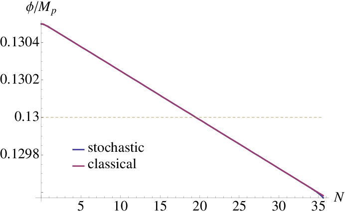
The time evolutions of the inflaton and waterfall field on one sample path with the initial condition are shown in figure 4 as “stochastic”. For the sake of comparison, we also plot the solution without noise as “classical”, with tiny but non-zero initial because the field with remains zero thereafter without noise. corresponds to the beginning of inflation. The waterfall field remains zero at first, because the mass of is as large as the Hubble parameter (or, is imaginary) and we omit the quantum noise as mentioned in the previous subsection. Subsequently, due to the noise, grows much rapidly compared with the classical solution. The inflaton field seems not to be affected by the noise term and its dynamics is almost same in both the stochastic and classical case. However, with the parameters in this paper, the end of inflation is determined by the value of . In fact, inflation without noise continues about 20 e-folds longer than stochastic inflation because the field value of does not grow fast without noise. It shows the importance of the stochastic effect not only for the calculation of the curvature perturbations but also the background dynamics. Note that, in both cases, the critical phase is reached about 20 e-folds after the beginning of the calculation.

In addition, let us check the time developments of the slow-roll parameters. In two-scalar inflation, there are following 5 slow-roll parameters.
| (38) |
The time developments of these slow-roll parameters for the sample path showed in figure 4 are illustrated in figure 5. exceeds unity first at and then slow-roll inflation ends.

In multi-field cases, the point where the slow-roll condition is violated is unsuitable for the end point of the field in the formula as we mentioned in the footnote of the previous section. That is because in multi-field inflation, slow-roll violating points are not on an equipotential line, though the end slice of the formula should be a uniform density slice. Therefore we use the uniform Hubble slice as the end. In figure 6, we show the contour plot of the potential with the sample path shown in figure 4 (red line) and uniform lines (dashed lines). It shows that equipotential lines do not correspond to uniform lines indeed. Parameters on the contour lines represent the value of . In this paper, we use (black thick line) as the end slice of formula where the slow-roll condition is violated enough as can be seen in figure 6.
Since above discussions are just for one sample path, one may doubt it depends on the sample paths. However, we checked that realizations
which quite deviate from this path and violate the above discussion almost never occur. Therefore it is valid to use
as the end slice.


|
Let us calculate the power spectrum of the curvature perturbations. Recalling the algorithm mentioned in section 3, we should make many sample paths from the fixed initial condition, which we have set at .1111 11 This initial value corresponds to as can be read from figure 4, though the initial condition should be set on the point which corresponds to our observable universe as we mentioned in section 3. However, in the valley phase, the mass of is heavy enough and rapidly converges to zero. Namely, the point is on an attractor. Therefore, without specifying the initial condition at , many sample paths converge to around this point. We can also rephrase it that we chose some initial condition at from which the sample paths converge to around the point . In this paper, for simplicity, and since we are interested only in around the critical point corresponding to , we calculate only about last 35 e-folds. For each sample path, we obtain a vs. plot taking “initial” values on that sample path. For example, we show vs. plot for one sample path in figure 7. Reiterating to solve the Langevin e.o.m. from one “initial” value on that sample path to the end of inflation, we can get the e-folds and the variance of them . Then, changing the “initial” value variously, full vs. plot such as the right panel of figure 7 can be obtained. In this paper, we reiterate the calculation 10000 times for each “initial” value.


|
Similarly, we can obtain many vs. plots for various sample paths. Then the true vs. plot of our observable universe is just the average of these plots. In the left panel of figure 8, we show the average of vs. plots for 10000 sample paths. Finally, differentiating this plot, we obtain the power spectrum of the curvature perturbations as shown in the right panel of figure 8. The horizontal axis corresponds to a wavenumber by the relation where is the horizon scale at the end of inflation, , and the scale corresponding to the critical point is for example. Figure 8 shows the peak of the power spectrum in the waterfall phase after the critical point because of the tachyonic instability of the waterfall field .
Not only in the hybrid case but also in any highly stochastic cases, we can calculate the power spectrum applying the stochastic- formalism shown here. Note that for the inflation models or parameters which we adopt, the variance of e-folds should not exceed unity in our observable universe, namely . For , the universe becomes too inhomogeneous to account for the observed universe. Indeed, the constraints from PBHs suggest for a wide range of and therefore [7, 8].
6 Conclusion
In this paper, we applied the non-perturbative method that we have proposed in the previous paper [1], the stochastic- formalism, to chaotic inflation and hybrid inflation. Especially, in hybrid inflation, we chose the parameters where the waterfall phase lasts for more than 10 e-folds, and calculated the power spectrum of the curvature perturbations including around the critical point. The result is shown in figure 3 and 8 for chaotic and hybrid inflation respectively. In particular, it is the first time that the power spectrum in hybrid inflation is calculated fully from the phase before the critical point to the end of inflation. The resultant power spectrum shows a peak profile due to the tachyonic instability of the waterfall field during the waterfall phase .
Though the recent CMB observations by the Planck and BICEP2 collaborations [3, 2] favor a simple single-large-field inflationary model, several multi-field models may be worth considering and they can have the highly stochastic region. In such cases, the method we demonstrated in this paper is needed to obtain the curvature perturbations.
Acknowledgements.
We would like to thank Ryo Namba for helpful discussions and advice. We also thank the authors of the publicly available distribution “Mersenne Twister” [51], which we used for generating the stochastic noise in the Langevin equations. This work is supported by Grant-in-Aid for Scientific research from the Ministry of Education, Science, Sports, and Culture (MEXT), Japan, No. 25400248 [MK], No. 21111006 [MK] and also by World Premier International Research Center Initiative (WPI Initiative), MEXT, Japan. T.F. acknowledges the support by JSPS Research Fellowships for Young Scientists. The work of Y.T. is partially supported by an Advanced Leading Graduate Course for Photon Science grant.Appendix A Numerical calculation of stochastic process
In this appendix, we comment on the numerical calculation method of the stochastic process. There are many numerical integrating methods with excellent converging properties like a Runge-Kutta method for ordinary differential equations, while the methods for stochastic differential equations like a Langevin equation are still developing. Since applying the method for ordinary differential equations to stochastic ones directly generally violate the desired properties of the stochastic process, specific methods should be constructed. We will give the terminology of stochastic calculus first, and then describe the numerical integrating method we used in this paper. Note that this appendix is based on ref. [49, 48].
A.1 Stochastic calculus
In the first place, let us define Brownian motion, which is the simplest stochastic process. Brownian motion is the continuous time limit of a random walk and mathematically defined as follows.
Definition A.1
Some stochastic continuous function is assumed to exist, satisfying . Then, if for all , the increments
| (39) |
are independent, Gaussian distributed and satisfy the condition,
| (40) |
is called Brownian motion.
The zero-mean white noise in the Langevin equation is formally defined as the derivative of Brownian motion:1212 12 Strictly speaking, Brownian motion is differentiable nowhere. The definition 41 is just a formal one.
| (41) |
Indeed, if has a white spectrum , this definition satisfies the condition 40 as follows.
| (42) | |||||
| (43) | |||||
Next, let us define the integral,
| (44) |
to integrate a Langevin equation. Here the integrand can generally depend on the past stochastic process. To define this integral, we will approximate the integrand by a simple process at first, and then take a limit.

In the first place, is defined as a partition of , namely
| (45) |
Then in each sub-period , the integrand is approximated by the constant function . In other words, is approximated by the initial value in each sub-period (see also figure 9). Generally, we can choose the partition for the approximation function to be closer to the integrand in the following sense.
| (46) |
Finally, with use of this approximation function, we define the integral (44) as
| (47) |
The integral defined by approximating the integrand by the initial value in each sub-period like above is called “Ito integral”. The point to notice is that the value of the stochastic integral can depend on where the integrand is approximated unlike the ordinary integral. The integral approximating the integrand by the midpoint value is called “Stratonovich integral” and its value can be different from that of Ito integral. However, we should use Ito integral for the noise during inflation because the noise amplitude should be evaluated just before the inflaton receives the noise, otherwise the causality is broken.
In this paper, all Langevin equations like
| (48) |
are defined as Ito integral,
| (49) |
In the next subsection, we will introduce the numerical integrations of Ito type.
A.2 Numerical method
In the numerical integration methods, the most standard one is a time discretization. For the Ito process
| (50) |
the simplest finite difference approximation is given by the Euler-Maruyama method:
| (51) |
where the initial value is and the step sizes are
| (52) |
In the viewpoint of the numerical integration, is a Gaussian distributed random variable whose expectation and variance are zero and respectively,
| (53) |
Next, let us mention the index of strong convergence.
Definition A.2
If for the numerical approximation of a stochastic process , there are some finite constant and positive constant satisfying
| (54) |
for any time partition whose maximum step size is , this approximation is said to converge strongly with order .
The convergence of stochastic process is generally bad and the order of the approximation for the stochastic differential equation is often smaller than that for the ordinary differential equation. In fact, though the order of the Euler-Maruyama approximation for the ordinary differential equation is , it has been proved that the order of that for the stochastic differential equation is .
Finally, we introduce the Runge-Kutta method for the stochastic differential equation. The Runge-Kutta method is quite practical since it can give stable solution even with a large step size. For the Ito process depending on independent -dimension Brownian motion,
| (55) |
The -staged Runge-Kutta is parameterized as follows generally.
| (56) | |||||
where,
| (57) |
and and are the method parameters. denotes the multiple Ito integral, and when noise correlations are represented as
| (58) |
it is written as
| (59) |
Especially for independent noise, reads the Kronecker delta . The parameters are often listed with use of the extended Butcher table 1. In table 2, we show the parameters of the 3-staged order 1.0 strong Runge-Kutta [50] which we use in this paper.
Appendix B Mixing
In this paper, the solutions with the constant masses (33), assuming the effect of the mass change during sub-horizon is negligible. However, the mixing term remains even in this case. Though we neglect this term in this paper, the effect of mixing can be taken as follows.
Here we treat as a constant and evaluate it at horizon crossing for each mode, even though it varies as time goes on actually. Taking the diagonalizing matrix of :
the field has no mixing. Therefore, the correlator of the original field reads,
| (64) |
and the following power spectrum should be used as the amplitude of noise .
| (65) |
Note that the summation with respect to is not taken. Noise also has non-zero correlation,
| (66) |
for . Here denotes the power spectrum given by eq. (65).
References
- (1) T. Fujita, M. Kawasaki, Y. Tada and T. Takesako, “A new algorithm for calculating the curvature perturbations in stochastic inflation,” JCAP 1312, 036 (2013) [arXiv:1308.4754 [astro-ph.CO]].
- (2) P. A. R. Ade et al. [BICEP2 Collaboration], “BICEP2 I: Detection Of B-mode Polarization at Degree Angular Scales,” arXiv:1403.3985 [astro-ph.CO].
- (3) P. A. R. Ade et al. [Planck Collaboration], “Planck 2013 results. XVI. Cosmological parameters,” arXiv:1303.5076 [astro-ph.CO].
- (4) B. J. Carr, “The Primordial black hole mass spectrum,” Astrophys. J. 201, 1 (1975).
- (5) B. J. Carr, “Some cosmological consequences of primordial black-hole evaporations,” Astrophys. J. 206, 8 (1976).
- (6) B. J. Carr, “Primordial black holes as a probe of cosmology and high energy physics,” Lect. Notes Phys. 631, 301 (2003) [astro-ph/0310838].
- (7) A. S. Josan, A. M. Green and K. A. Malik, “Generalised constraints on the curvature perturbation from primordial black holes,” Phys. Rev. D 79, 103520 (2009) [arXiv:0903.3184 [astro-ph.CO]].
- (8) B. J. Carr, K. Kohri, Y. Sendouda and J. ’i. Yokoyama, “New cosmological constraints on primordial black holes,” Phys. Rev. D 81, 104019 (2010) [arXiv:0912.5297 [astro-ph.CO]].
- (9) A. S. Josan and A. M. Green, “Gamma-rays from ultracompact minihalos: potential constraints on the primordial curvature perturbation,” Phys. Rev. D 82, 083527 (2010) [arXiv:1006.4970 [astro-ph.CO]].
- (10) T. Bringmann, P. Scott and Y. Akrami, “Improved constraints on the primordial power spectrum at small scales from ultracompact minihalos,” Phys. Rev. D 85, 125027 (2012) [arXiv:1110.2484 [astro-ph.CO]].
- (11) F. Li, A. L. Erickcek and N. M. Law, “A new probe of the small-scale primordial power spectrum: astrometric microlensing by ultracompact minihalos,” Phys. Rev. D 86, 043519 (2012) [arXiv:1202.1284 [astro-ph.CO]].
- (12) A. A. Starobinsky, “Stochastic De Sitter (inflationary) Stage In The Early Universe,” In *De Vega, H.j. ( Ed.), Sanchez, N. ( Ed.): Field Theory, Quantum Gravity and Strings*, 107-126 (1986).
- (13) M. Sasaki, Y. Nambu and K. -i. Nakao, “Classical Behavior Of A Scalar Field In The Inflationary Universe,” Nucl. Phys. B 308, 868 (1988).
- (14) K. -i. Nakao, Y. Nambu and M. Sasaki, “Stochastic Dynamics Of New Inflation,” Prog. Theor. Phys. 80, 1041 (1988).
- (15) Y. Nambu and M. Sasaki, “Stochastic Approach To Chaotic Inflation And The Distribution Of Universes,” Phys. Lett. B 219, 240 (1989).
- (16) S. Mollerach, S. Matarrese, A. Ortolan and F. Lucchin, “Stochastic inflation in a simple two field model,” Phys. Rev. D 44, 1670 (1991).
- (17) A. A. Starobinsky and J. Yokoyama, “Equilibrium state of a selfinteracting scalar field in the De Sitter background,” Phys. Rev. D 50, 6357 (1994) [astro-ph/9407016].
- (18) F. Finelli, G. Marozzi, A. A. Starobinsky, G. P. Vacca and G. Venturi, “Generation of fluctuations during inflation: Comparison of stochastic and field-theoretic approaches,” Phys. Rev. D 79, 044007 (2009) [arXiv:0808.1786 [hep-th]].
- (19) F. Finelli, G. Marozzi, A. A. Starobinsky, G. P. Vacca and G. Venturi, “Stochastic growth of quantum fluctuations during slow-roll inflation,” Phys. Rev. D 82, 064020 (2010) [arXiv:1003.1327 [hep-th]].
- (20) K. Enqvist, D. G. Figueroa and G. Rigopoulos, “Fluctuations along supersymmetric flat directions during Inflation,” JCAP 1201, 053 (2012) [arXiv:1109.3024 [astro-ph.CO]].
- (21) M. Kawasaki and T. Takesako, “Stochastic Approach to Flat Direction during Inflation,” JCAP 1208, 031 (2012).
- (22) J. C. B. Sanchez and K. Enqvist, “On the fate of coupled flat directions during inflation,” JCAP 1303 (2013) 029 [arXiv:1210.7007 [astro-ph.CO]].
- (23) J. C. B. Sanchez and K. Dimopoulos, “Inflationary buildup of a vector field condensate and its cosmological consequences,” arXiv:1308.3739 [hep-ph].
- (24) A. A. Starobinsky, “Multicomponent de Sitter (Inflationary) Stages and the Generation of Perturbations,” JETP Lett. 42, 152 (1985) [Pisma Zh. Eksp. Teor. Fiz. 42, 124 (1985)].
- (25) D. S. Salopek and J. R. Bond, “Nonlinear evolution of long wavelength metric fluctuations in inflationary models,” Phys. Rev. D 42, 3936 (1990).
- (26) M. Sasaki and E. D. Stewart, “A General analytic formula for the spectral index of the density perturbations produced during inflation,” Prog. Theor. Phys. 95, 71 (1996) [astro-ph/9507001].
- (27) M. Sasaki and T. Tanaka, “Superhorizon scale dynamics of multiscalar inflation,” Prog. Theor. Phys. 99, 763 (1998) [gr-qc/9801017].
- (28) D. H. Lyth, K. A. Malik and M. Sasaki, “A General proof of the conservation of the curvature perturbation,” JCAP 0505, 004 (2005) [astro-ph/0411220].
- (29) A. D. Linde, “Chaotic Inflation,” Phys. Lett. B 129, 177 (1983).
- (30) A. D. Linde, “Hybrid inflation,” Phys. Rev. D 49, 748 (1994) [astro-ph/9307002].
- (31) E. J. Copeland, A. R. Liddle, D. H. Lyth, E. D. Stewart and D. Wands, “False vacuum inflation with Einstein gravity,” Phys. Rev. D 49, 6410 (1994) [astro-ph/9401011].
- (32) S. Clesse and J. Rocher, “Avoiding the blue spectrum and the fine-tuning of initial conditions in hybrid inflation,” Phys. Rev. D 79, 103507 (2009) [arXiv:0809.4355 [hep-ph]].
- (33) S. Clesse, “Hybrid inflation along waterfall trajectories,” Phys. Rev. D 83, 063518 (2011) [arXiv:1006.4522 [gr-qc]].
- (34) G. R. Dvali, Q. Shafi and R. K. Schaefer, “Large scale structure and supersymmetric inflation without fine tuning,” Phys. Rev. Lett. 73, 1886 (1994) [hep-ph/9406319].
- (35) P. Binetruy and G. R. Dvali, “D term inflation,” Phys. Lett. B 388, 241 (1996) [hep-ph/9606342].
- (36) E. Halyo, “Hybrid inflation from supergravity D terms,” Phys. Lett. B 387, 43 (1996) [hep-ph/9606423].
- (37) R. Kallosh and A. D. Linde, “P term, D term and F term inflation,” JCAP 0310, 008 (2003) [hep-th/0306058].
- (38) D. H. Lyth, “Contribution of the hybrid inflation waterfall to the primordial curvature perturbation,” JCAP 1107, 035 (2011) [arXiv:1012.4617 [astro-ph.CO]].
- (39) D. H. Lyth, “The hybrid inflation waterfall and the primordial curvature perturbation,” JCAP 1205, 022 (2012) [arXiv:1201.4312 [astro-ph.CO]].
- (40) M. Morikawa, “Dissipation and Fluctuation of Quantum Fields in Expanding Universes,” Phys. Rev. D 42, 1027 (1990).
- (41) P. Ivanov, “Nonlinear metric perturbations and production of primordial black holes,” Phys. Rev. D 57, 7145 (1998) [astro-ph/9708224].
- (42) J. ’i. Yokoyama, “Chaotic new inflation and formation of primordial black holes,” Phys. Rev. D 58, 083510 (1998) [astro-ph/9802357].
- (43) K. E. Kunze, “Perturbations in stochastic inflation,” JCAP 0607, 014 (2006) [astro-ph/0603575].
- (44) K. Enqvist, S. Nurmi, D. Podolsky and G. I. Rigopoulos, JCAP 0804, 025 (2008) [arXiv:0802.0395 [astro-ph]].
- (45) R. Saito, J. ’i. Yokoyama and R. Nagata, “Single-field inflation, anomalous enhancement of superhorizon fluctuations, and non-Gaussianity in primordial black hole formation,” JCAP 0806, 024 (2008) [arXiv:0804.3470 [astro-ph]].
- (46) L. Perreault Levasseur, “Lagrangian Formulation of Stochastic Inflation: A Recursive Approach,” arXiv:1304.6408 [hep-th].
- (47) L. Perreault Levasseur, V. Vennin and R. Brandenberger, “Recursive Stochastic Effects in Valley Hybrid Inflation,” arXiv:1307.2575 [hep-th].
- (48) P. E. Kloeden and E. Platen, “Numerical Solution of Stochastic Differential Equations,” Springer-Verlag, New York (1992) 632 p.
- (49) S. E. Shreve, “Stochastic Calculus for Finance II: Continuous-Time Models,” Springer-Verlag, New York (2004) 550 p.
- (50) A. Rößler, “Runge-Kutta methods for the strong approximation of solutions of stochastic differential equations,” SIAM Journal on Numerical Analysis 48.3 (2010): 922-952.
- (51) M. Matsumoto and T. Nishimura, “Mersenne twister: a 623-dimensionally equidistributed uniform pseudo-random number generator,” ACM Transactions on Modeling and Computer Simulation (TOMACS) 8.1 (1998): 3-30.