跳到论文正文
W Papers独立论文阅读器 arXiv:1405.2140 论文正文 计算阅读时间 · 0%
引用这篇论文根据当前论文元数据生成,正式投稿前建议核对。


License: arXiv.org perpetual non-exclusive license
arXiv:1405.2140v1 [math.NA] 09 May 2014

Time-stepping error bounds for fractional diffusion problems with non-smooth initial data

William McLean Email: w.mclean@unsw.edu.au Address: School of Mathematics and Statistics, The University of New South Wales, Sydney 2052, Australia Note: We thank the Australian Research Council and the summer visit program of the KFUPM for their financial support of this project. Note: The first author completed part of this research during an extended visit to the University of Otago, Dunedin.    Kassem Mustapha Email: kassem@kfupm.edu.sa Address: Department of Mathematics and Statistics, King Fahd University of Petroleum and Minerals, Dhahran, 31261, Saudi Arabia Note: We thank the Australian Research Council and the summer visit program of the KFUPM for their financial support of this project.
Abstract

We apply the piecewise constant, discontinuous Galerkin method to discretize a fractional diffusion equation with respect to time. Using Laplace transform techniques, we show that the method is first order accurate at the nnth time level tnt_{n}, but the error bound includes a factor tn−1t_{n}^{-1} if we assume no smoothness of the initial data. We also show that for smoother initial data the growth in the error bound as tnt_{n} decreases is milder, and in some cases absent altogether. Our error bounds generalize known results for the classical heat equation and are illustrated for a model problem.

Keywords: 
Discontinuous Galerkin method, implicit Euler method, Laplace transform, polylogarithm.
2010 MSC
65M15, 35R11, 45K05, 44A10.

1 Introduction

Consider an initial-value problem for an abstract, time-fractional diffusion equation [7, p. 84]

∂tu+∂t1−νA​u=0for t>0,with u⁡(0)=u0 and 0<ν<1.\partial_{t}u+\partial_{t}^{1-\nu}Au=0\quad\text{for $t>0$,}\quad\text{with $u(0)=u_{0}$ and $0<\nu<1$.} (1)

Here, we think of the solution uu as a function from [0,∞)[0,\infty) to a Hilbert space ℋ\mathcal{H}, with ∂tu=u′​(t)\partial_{t}u=u^{\prime}(t) the usual derivative with respect to tt, and with

∂t1−νu⁡(t)=∂∂t​∫0t(t−s)ν−1Γ⁡(ν)​u​(s)​𝑑s\partial_{t}^{1-\nu}u(t)=\frac{\partial}{\partial t}\int_{0}^{t}\frac{(t-s)^{\nu-1}}{\Gamma(\nu)}\,u(s)\,ds

the Riemann–Liouville fractional derviative of order 1−ν1-\nu. The linear operator AA is assumed to be self-adjoint, positive-semidefinite and densely defined in ℋ\mathcal{H}, with a complete orthonormal eigensystem ϕ1\phi_{1}, ϕ2\phi_{2}, ϕ3\phi_{3}, …. We further assume that the eigenvalues of AA tend to infinity. Thus,

A​ϕm=λm​ϕm,⟨ϕm,ϕn⟩=δm​n,0≤λ1≤λ2≤λ3≤⋯,A\phi_{m}=\lambda_{m}\phi_{m},\quad\langle\phi_{m},\phi_{n}\rangle=\delta_{mn},\quad 0\leq\lambda_{1}\leq\lambda_{2}\leq\lambda_{3}\leq\cdots,

where ⟨u,v⟩\langle u,v\rangle is the inner product in ℋ\mathcal{H}; the corresponding norm in ℋ\mathcal{H} is denoted by ‖u‖=⟨u,u⟩\|u\|=\sqrt{\langle u,u\rangle}. In particular, we may take A​u=−∇2uAu=-\nabla^{2}u and ℋ=L2​(Ω)\mathcal{H}=L_{2}(\Omega) for a bounded spatial domain Ω\Omega, with uu subject to homogeneous Dirichlet or Neumann boundary conditions on ∂Ω\partial\Omega. Our problem (1) then reduces to the classical heat equation when ν→1\nu\to 1.

Many authors have studied techniques for the time discretization of (1), but obtaining sharp error bounds has proved challenging. In studies of explicit and implicit finite difference schemes [1, 3, 8, 14, 17, 20] the error analyses typically assume that the solution u⁡(t)u(t) is sufficiently smooth, including at t=0t=0, which amounts to imposing compatibility conditions on the initial data and source term. In our earlier work on discontinuous Galerkin (DG) time-stepping [11, 15, 16], we permitted more realistic behaviour, allowing the derivatives of u⁡(t)u(t) to be unbounded as t→0t\to 0, but were seeking error bounds that are uniform in tt using variable time steps. In the present work, we again consider a piecewise-constant DG scheme but with a completely different method of analysis that leads to sharp error bounds even for non-smooth initial data, at the cost of requiring a constant time step Δ​t\Delta t. Our previous analysis [11, Theorem 5] of the scheme (5), in conjunction with relevant estimates [10] of the derivatives of uu, shows, in the special case of uniform time steps, only the sub-optimal error bound

‖Un−u⁡(tn)‖≤C​Δ​tr​ν​‖Ar​u0‖for 0≤r<1/ν.\|U^{n}-u(t_{n})\|\leq C\Delta t^{r\nu}\|A^{r}u_{0}\|\quad\text{for $0\leq r<1/\nu$.} (2)

In our main result, we substantially improve on (2) by showing that

‖Un−u⁡(tn)‖≤C​tnr​ν−1​Δ​t​‖Ar​u0‖for 0≤r≤min⁡(2,1/ν).\|U^{n}-u(t_{n})\|\leq Ct_{n}^{r\nu-1}\Delta t\|A^{r}u_{0}\|\quad\text{for $0\leq r\leq\min(2,1/\nu)$.} (3)

Thus, for a general u0∈ℋu_{0}\in\mathcal{H} the error is of order tn−1​Δ​tt_{n}^{-1}\Delta t at t=tnt=t_{n}, so the method is first-order accurate but the error bound includes a factor tn−1t_{n}^{-1} that grows if tnt_{n} approaches zero, until at t=t1t=t_{1} the bound is of order t1−1​Δ​t=1t_{1}^{-1}\Delta t=1. However, if 1/2≤ν<11/2\leq\nu<1 and u0u_{0} is smooth enough to belong to D⁡(A1/ν)D(A^{1/\nu}), the domain of A1/νA^{1/\nu}, then the error is of order Δ​t\Delta t, uniformly in tnt_{n}. For 0<ν≤1/20<\nu\leq 1/2, no matter how smooth u0u_{0} a factor tn2​r−1t_{n}^{2r-1} is present. To the best of our knowledge, only Cuesta et al. [2] and McLean and Thomée [12, Theorem 3.1] have hitherto investigated the time discretization of (1) for the interesting case when the initial data might not be regular, the former using a finite difference-convolution quadrature scheme and the latter a method based on numerical inversion of the Laplace transform.

In the present work, we do not discuss the spatial discretization of (1). By contrast, Jin, Lazarov and Zhou [6] applied a piecewise linear finite element method using a quasi-uniform partition of Ω\Omega into elements with maximum diameter hh, but with no time discretization. They worked with an equivalent formulation of the fractional diffusion problem,

∂t,Cνu−∇2u=0for x∈Ω and 0<t≤T,\partial_{t,\text{C}}^{\nu}u-\nabla^{2}u=0\quad\text{for $x\in\Omega$ and $0<t\leq T$,} (4)

where ∂t,C\partial_{t,\text{C}} denotes the Caputo fractional derivative, and proved [6, Theorems 3.5 and 3.7] that, for an appropriate choice of uh​(0)u_{h}(0),

‖uh​(t)−u⁡(t)‖+h​‖∇(uh−u)‖≤C​tν⁡(r−1)×{h2​ℓh​‖Ar​u0‖,r∈{0,1/2},h2​‖Ar​u0‖,r=1,\|u_{h}(t)-u(t)\|+h\|\nabla(u_{h}-u)\|\leq Ct^{\nu(r-1)}\times\begin{cases}h^{2}\ell_{h}\|A^{r}u_{0}\|,&r\in\{0,1/2\},\\ h^{2}\|A^{r}u_{0}\|,&r=1,\end{cases}

where ℓh=max⁡(1,log⁡h−1)\ell_{h}=\max(1,\log h^{-1}). These estimates for the spatial error complement our bounds for the error in a time discretization.

For a fixed step size Δ​t>0\Delta t>0, we put tn=n​Δ​tt_{n}=n\Delta t and define a piecewise-constant approximation U⁡(t)≈u⁡(t)U(t)\approx u(t) by applying the DG method [11, 13],

Un−Un−1+∫tn−1tn∂t1−νA​U​(t)​𝑑t=0for n≥1, with U0=u0,U^{n}-U^{n-1}+\int_{t_{n-1}}^{t_{n}}\partial_{t}^{1-\nu}AU(t)\,dt=0\quad\text{for $n\geq 1$, with $U^{0}=u_{0}$,} (5)

where Un=U⁡(tn−)=limt→tn−U⁡(t)U^{n}=U(t_{n}^{-})=\lim_{t\to t_{n}^{-}}U(t) denotes the one-sided limit from below at the nnth time level. Thus, U⁡(t)=UnU(t)=U^{n} for tn−1<t≤tnt_{n-1}<t\leq t_{n}. Since we do not consider any spatial discretization, UU is a semidiscrete solution with values in ℋ\mathcal{H}. A short calculation reveals that

∫tn−1tn∂t1−νA​U​(t)​𝑑t=Δ​tν​∑j=1nβn−j​A​Uj,\int_{t_{n-1}}^{t_{n}}\partial_{t}^{1-\nu}AU(t)\,dt=\Delta t^{\nu}\sum_{j=1}^{n}\beta_{n-j}AU^{j},

with

β0=Δ​t−ν​∫tn−1tn(tn−t)ν−1Γ⁡(ν)​𝑑t=1Γ⁡(1+ν)\beta_{0}=\Delta t^{-\nu}\int_{t_{n-1}}^{t_{n}}\frac{(t_{n}-t)^{\nu-1}}{\Gamma(\nu)}\,dt=\frac{1}{\Gamma(1+\nu)}

and, for j≥1j\geq 1,

βj=Δ​t−ν​∫tn−j−1tn−j(tn−t)ν−1−(tn−1−t)ν−1Γ⁡(ν)​𝑑t=(j+1)ν−2​jν+(j−1)νΓ⁡(1+ν).\beta_{j}=\Delta t^{-\nu}\int_{t_{n-j-1}}^{t_{n-j}}\frac{(t_{n}-t)^{\nu-1}-(t_{n-1}-t)^{\nu-1}}{\Gamma(\nu)}\,dt=\frac{(j+1)^{\nu}-2j^{\nu}+(j-1)^{\nu}}{\Gamma(1+\nu)}.

Thus, by solving the recurrence relation

(I+β0​Δ​tν​A)​Un=Un−1−Δ​tν​∑j=1n−1βn−j​A​Uj(I+\beta_{0}\Delta t^{\nu}A)U^{n}=U^{n-1}-\Delta t^{\nu}\sum_{j=1}^{n-1}\beta_{n-j}AU^{j} (6)

for n=1n=1, 22, 33, …we may compute U1U^{1}, U2U^{2}, U3U^{3}, ….

In the classical limit as ν→1\nu\to 1, the fractional-order equation (1) reduces to an abstract heat equation,

∂tu+A​u=0for t>0,with u⁡(0)=u0,\partial_{t}u+Au=0\quad\text{for $t>0$,}\quad\text{with $u(0)=u_{0}$,} (7)

and the time-stepping DG method (5) reduces to the implicit Euler scheme

Un−Un−1Δ​t+A​Un=0,\frac{U^{n}-U^{n-1}}{\Delta t}+AU^{n}=0, (8)

for which the following error bound holds [18, Theorems 7.1 and 7.2]:

‖Un−u⁡(tn)‖≤C​tnr−1​Δ​t​‖Ar​u0‖for n=1, 2, 3, …and 0≤r≤1.\|U^{n}-u(t_{n})\|\leq Ct_{n}^{r-1}\Delta t\|A^{r}u_{0}\|\quad\text{for $n=1$, $2$, $3$, \ldots and $0\leq r\leq 1$.} (9)

This result is just the limiting case as ν→1\nu\to 1 of our error estimate (3) for the fractional diffusion equation.

For any real r≥0r\geq 0, we can characterize D⁡(Ar)D(A^{r}) in terms of the generalized Fourier coefficients in an eigenfunction expansion,

v=∑m=1∞vm​ϕm,vm=⟨v,ϕm⟩.v=\sum_{m=1}^{\infty}v_{m}\phi_{m},\quad v_{m}=\langle v,\phi_{m}\rangle.

Indeed, v∈ℋv\in\mathcal{H} belongs to D⁡(Ar)D(A^{r}) if and only if

‖Ar​v‖2=∑m=1∞λm2​r​vm2<∞,\|A^{r}v\|^{2}=\sum_{m=1}^{\infty}\lambda_{m}^{2r}v_{m}^{2}<\infty, (10)

in which case the series Ar​v=∑m=1∞λmr​vm​ϕmA^{r}v=\sum_{m=1}^{\infty}\lambda_{m}^{r}v_{m}\phi_{m} converges in ℋ\mathcal{H}. Thus (recalling our assumption that λm→∞\lambda_{m}\to\infty) the larger the value of rr such that v∈D⁡(Ar)v\in D(A^{r}), the faster the Fourier coefficients vmv_{m} decay as m→∞m\to\infty and the “smoother” vv is. When ℋ=L2​(Ω)\mathcal{H}=L_{2}(\Omega) the functions in D⁡(Ar)D(A^{r}) may have to satisfy compatibility conditions on ∂Ω\partial\Omega; see Thomée [18, Lemma 3.1] or [10, Section 3]. In particular, an infinitely differentiable function will be somewhat “non-smooth” if it fails to satisfy the boundary conditions of our problem.

We note that, for a given u0u_{0}, the exact solution uu is less smooth than is the case for the classical heat equation. To see why, consider the Fourier expansion

u⁡(t)=∑m=1∞um​(t)​ϕm,um​(t)=⟨u⁡(t),ϕm⟩,u(t)=\sum_{m=1}^{\infty}u_{m}(t)\phi_{m},\qquad u_{m}(t)=\langle u(t),\phi_{m}\rangle, (11)

and put u0​m=⟨u0,ϕm⟩u_{0m}=\langle u_{0},\phi_{m}\rangle. The Fourier coefficients um​(t)u_{m}(t) satisfy the initial-value problem

um′+λm​∂t1−νum=0,for t>0, with um​(0)=u0​m,u_{m}^{\prime}+\lambda_{m}\partial_{t}^{1-\nu}u_{m}=0,\quad\text{for~$t>0$, with $u_{m}(0)=u_{0m}$,} (12)

so that, as is well known [10], um​(t)=Eν​(−λm​tν)​u0​mu_{m}(t)=E_{\nu}(-\lambda_{m}t^{\nu})u_{0m} where EνE_{\nu} denotes the Mittag–Leffler function. Since Eν​(−s)=O⁡(s−1)E_{\nu}(-s)=O(s^{-1}) decays slowly as s→∞s\to\infty for 0<ν<10<\nu<1, in comparison to E1​(−s)=e−sE_{1}(-s)=e^{-s}, the high frequency modes of the solution are not damped as rapidly as in the classical case ν=1\nu=1.

Section 2 uses Laplace transform techniques to derive integral representations for the Fourier coefficients Umn=⟨Un,ϕm⟩U^{n}_{m}=\langle U^{n},\phi_{m}\rangle and um​(tn)=⟨u⁡(tn),ϕm⟩u_{m}(t_{n})=\langle u(t_{n}),\phi_{m}\rangle. We show that Umn−um​(tn)=δn​(μ)​u0​mU^{n}_{m}-u_{m}(t_{n})=\delta^{n}(\mu)u_{0m}, where δn​(μ)\delta^{n}(\mu) is given by an explicit but complicated integral; thus, the error has a Fourier expansion of the form

Un−u⁡(tn)=∑m=1∞δn​(λm​Δ​tν)​u0​m​ϕm,u0​m=⟨u0,ϕm⟩.U^{n}-u(t_{n})=\sum_{m=1}^{\infty}\delta^{n}(\lambda_{m}\Delta t^{\nu})u_{0m}\phi_{m},\quad u_{0m}=\langle u_{0},\phi_{m}\rangle. (13)

Theorem 4 states a key estimate for δn​(μ)\delta^{n}(\mu), but to avoid a lengthy digression the proof is relegated to Section 4.

The main result (3) of the paper is established in Section 3, where we first prove in Theorem 5 that if u0∈ℋu_{0}\in\mathcal{H} then the error is of order tn−1​Δ​tt_{n}^{-1}\Delta t, coinciding with the error estimate (9) for the classical heat equation when r=0r=0. Next we prove the special case r=min⁡(2,1/ν)r=\min(2,1/\nu) of (3) and then, in Theorem 7, deduce the general case by interpolation. The paper concludes with Section 5, which presents the results of some computational experiments for a model 1D problem, as well as numerical evidence that the constant CC in (3) can be chosen independent of ν\nu.

2 Integral representations

Our error analysis relies on the Laplace transform

u^​(z)=ℒ⁡{u⁡(t)}=∫0∞e−z​t​u​(t)​𝑑t.\hat{u}(z)=\mathcal{L}\{u(t)\}=\int_{0}^{\infty}e^{-zt}u(t)\,dt.

A standard energy argument [11, 13] shows that ‖u⁡(t)‖≤‖u0‖\|u(t)\|\leq\|u_{0}\| so u^​(z)\hat{u}(z) exists and is analytic in the right half-plane ℜ⁡z>0\Re z>0, and since ℒ⁡{∂t1−νu}=z1−ν​u^​(z)\mathcal{L}\{\partial_{t}^{1-\nu}u\}=z^{1-\nu}\hat{u}(z) and ℒ⁡{∂tu}=z​u^−u0\mathcal{L}\{\partial_{t}u\}=z\hat{u}-u_{0}, it follows from (12) that z​u^m+λm​z1−ν​u^m=u0​mz\hat{u}_{m}+\lambda_{m}z^{1-\nu}\hat{u}_{m}=u_{0m}, so

u^m​(z)=u0​mz+λm​z1−ν.\hat{u}_{m}(z)=\frac{u_{0m}}{z+\lambda_{m}z^{1-\nu}}.

Thus, the Laplace inversion formula gives, for n≥1n\geq 1 and any a>0a>0,

um​(tn)=12​π​i​∫a−i​∞a+i​∞ez​tn​u^m​(z)​𝑑z=u0​m2​π​i​∫a−i​∞a+i​∞ez​tn1+λm​z−ν​d​zz,u_{m}(t_{n})=\frac{1}{2\pi i}\int_{a-i\infty}^{a+i\infty}e^{zt_{n}}\hat{u}_{m}(z)\,dz=\frac{u_{0m}}{2\pi i}\int_{a-i\infty}^{a+i\infty}\frac{e^{zt_{n}}}{1+\lambda_{m}z^{-\nu}}\,\frac{dz}{z},

which, following a substitution, we may write as

um​(tn)=u0​m2​π​i​∫a−i​∞a+i​∞en​z1+μ​z−ν​d​zz,where μ=λm​Δ​tν.u_{m}(t_{n})=\frac{u_{0m}}{2\pi i}\int_{a-i\infty}^{a+i\infty}\frac{e^{nz}}{1+\mu z^{-\nu}}\,\frac{dz}{z},\quad\text{where $\mu=\lambda_{m}\Delta t^{\nu}$.} (14)

It follows using Jordan’s lemma that

um​(tn)=u0​m2​π​i​∫−∞0+en​z1+μ​z−ν​d​zzfor n≥1,u_{m}(t_{n})=\frac{u_{0m}}{2\pi i}\int_{-\infty}^{0^{+}}\frac{e^{nz}}{1+\mu z^{-\nu}}\,\frac{dz}{z}\quad\text{for $n\geq 1$,} (15)

where the notation ∫−∞0+\int_{-\infty}^{0^{+}} indicates that the path of integration is a Hankel contour enclosing the negative real axis and oriented counterclockwise.

Now consider the recurrence relation (6) used to compute the numerical solution. The Fourier coefficients Umn=⟨Un,ϕm⟩U^{n}_{m}=\langle U^{n},\phi_{m}\rangle satisfy

(1+β0​Δ​tν​λm)​Umn=Umn−1−λm​Δ​tν​∑j=1n−1βn−j​Umj,(1+\beta_{0}\Delta t^{\nu}\lambda_{m})U^{n}_{m}=U^{n-1}_{m}-\lambda_{m}\Delta t^{\nu}\sum_{j=1}^{n-1}\beta_{n-j}U^{j}_{m}, (16)

and to obtain an integral representation of UmnU^{n}_{m} analogous to (15) we introduce the discrete-time Laplace transform

U~​(z)=∑n=0∞Un​e−n​z.\widetilde{U}(z)=\sum_{n=0}^{\infty}U^{n}e^{-nz}. (17)

Again, a standard energy argument shows that ‖Un‖≤‖u0‖\|U^{n}\|\leq\|u_{0}\| so this series converges in the right half-plane ℜ⁡z>0\Re z>0. Multiplying (16) by e−n​ze^{-nz}, summing over nn and using the fact that the sum in (16) is a discrete convolution, we find that

[1−e−z+μ​β~​(z)]​U~m​(z)=[1+μ​β~​(z)]​u0​m,\bigl[1-e^{-z}+\mu\tilde{\beta}(z)\bigr]\widetilde{U}_{m}(z)=\bigl[1+\mu\tilde{\beta}(z)\bigr]u_{0m},

again with μ=λm​Δ​tν\mu=\lambda_{m}\Delta t^{\nu}. So, letting ψ⁡(z)=β~​(z)/(1−e−z)\psi(z)=\tilde{\beta}(z)/(1-e^{-z}),

U~m​(z)=u0​m​1+μ​β~​(z)1−e−z+μ​β~​(z)=u0​m​(1−e−z)−1+μ​ψ​(z)1+μ​ψ​(z).\widetilde{U}_{m}(z)=u_{0m}\,\frac{1+\mu\tilde{\beta}(z)}{1-e^{-z}+\mu\tilde{\beta}(z)}=u_{0m}\,\frac{(1-e^{-z})^{-1}+\mu\psi(z)}{1+\mu\psi(z)}. (18)

For our subsequent analysis we now establish key properties of the function ψ⁡(z)\psi(z).

Following appropriate shifts of the summation index, one finds that

β~​(z)=∑n=0∞βn​e−n​z=(ez−1)​(1−e−z)​Li−ν⁡(e−z)Γ⁡(1+ν),\tilde{\beta}(z)=\sum_{n=0}^{\infty}\beta_{n}e^{-nz}=(e^{z}-1)(1-e^{-z})\,\frac{\operatorname{Li}_{-\nu}(e^{-z})}{\Gamma(1+\nu)}, (19)

where the polylogarithm [9, 19] is defined by Lip⁡(z)=∑n=1∞zn/np\operatorname{Li}_{p}(z)=\sum_{n=1}^{\infty}z^{n}/n^{p} for |z|<1|z|<1 and p∈ℂp\in\mathbb{C}; thus,

ψ⁡(z)=(ez−1)​Li−ν⁡(e−z)Γ⁡(1+ν)=1Γ⁡(1+ν)​(1+∑n=1∞[(n+1)ν−nν]​e−n​z).\psi(z)=(e^{z}-1)\,\frac{\operatorname{Li}_{-\nu}(e^{-z})}{\Gamma(1+\nu)}=\frac{1}{\Gamma(1+\nu)}\biggl(1+\sum_{n=1}^{\infty}\bigl[(n+1)^{\nu}-n^{\nu}\bigr]e^{-nz}\biggr). (20)

From the identity

1np=Γ⁡(1−p)2​π​i​∫−∞0+en​w​wp−1​𝑑w,\frac{1}{n^{p}}=\frac{\Gamma(1-p)}{2\pi i}\int_{-\infty}^{0^{+}}e^{nw}w^{p-1}\,dw,

we find, after interchanging the sum and integral, that

Lip⁡(e−z)=Γ⁡(1−p)2​π​i​∫−∞0+wp−1​d​wez−w−1\operatorname{Li}_{p}(e^{-z})=\frac{\Gamma(1-p)}{2\pi i}\int_{-\infty}^{0^{+}}\frac{w^{p-1}\,dw}{e^{z-w}-1} (21)

for ℜ⁡z\Re z sufficiently large. Thus, Lip⁡(e−z)\operatorname{Li}_{p}(e^{-z}) possesses an analytic continuation to the strip −2​π<ℑ⁡z<2​π-2\pi<\Im z<2\pi with a cut along the negative real axis (−∞,0](-\infty,0]. It follows that ψ⁡(z)\psi(z) is analytic for zz in the same cut strip, and moreover

ψ⁡(z)¯=ψ⁡(z¯)andψ⁡(z+2​π​i)=ψ⁡(z).\overline{\psi(z)}=\psi(\bar{z})\quad\text{and}\quad\psi(z+2\pi i)=\psi(z). (22)
Lemma 1.

If |ℑ⁡z|≤π|\Im z|\leq\pi and z∉(−∞,0]z\notin(-\infty,0], then

ψ⁡(z)=sin⁡π​νπ​∫0∞s−ν1−e−z−s​1−e−ss​𝑑s\psi(z)=\frac{\sin\pi\nu}{\pi}\int_{0}^{\infty}\frac{s^{-\nu}}{1-e^{-z-s}}\,\frac{1-e^{-s}}{s}\,ds (23)

and 1+μ​ψ​(z)≠01+\mu\psi(z)\neq 0 for 0<μ<∞0<\mu<\infty.

Proof.

Given z∉(−∞,0]z\notin(-\infty,0], we can choose a Hankel contour that does not enclose zz, and the formulae (20) and (21) then imply that

ψ⁡(z)=ez−12​π​i​∫−∞0+w−ν−1​d​wez−w−1.\psi(z)=\frac{e^{z}-1}{2\pi i}\int_{-\infty}^{0^{+}}\frac{w^{-\nu-1}\,dw}{e^{z-w}-1}.

Since

ez−1ez−w−1=1+ew−11−ew−zand∫−∞0+w−ν−1​𝑑w=0,\frac{e^{z}-1}{e^{z-w}-1}=1+\frac{e^{w}-1}{1-e^{w-z}}\quad\text{and}\quad\int_{-\infty}^{0^{+}}w^{-\nu-1}\,dw=0,

we have

ψ⁡(z)=12​π​i​∫−∞0+w−ν1−ew−z​ew−1w​𝑑w.\psi(z)=\frac{1}{2\pi i}\int_{-\infty}^{0^{+}}\frac{w^{-\nu}}{1-e^{w-z}}\,\frac{e^{w}-1}{w}\,dw.

Define contours along either side of the cut,

𝒞±={s​e±i​π:for 0<s<∞},\mathcal{C}_{\pm}=\{\,se^{\pm i\pi}:\text{for $0<s<\infty$}\,\}, (24)

so that arg⁡(w)=±π\arg(w)=\pm\pi if w∈𝒞±w\in\mathcal{C}_{\pm}. Noting that the integrand is O⁡(w−ν)O(w^{-\nu}) as w→0w\to 0, we may collapse the Hankel contour into 𝒞+−𝒞−\mathcal{C}^{+}-\mathcal{C}^{-} to obtain (23).

The second part of the lemma amounts to showing that ψ(z)∉(−∞,0]\psi(z)\notin(-\infty,0]. If x≥0x\geq 0 and αn=e−x​n​[(n+1)ν−nν]\alpha_{n}=e^{-xn}\bigl[(n+1)^{\nu}-n^{\nu}\bigr], then

ψ⁡(x+i​y)=1Γ⁡(1+ν)​(1+∑n=1∞αn​cos⁡n​y−i​∑n=1∞αn​sin⁡n​y).\psi(x+iy)=\frac{1}{\Gamma(1+\nu)}\biggl(1+\sum_{n=1}^{\infty}\alpha_{n}\cos ny-i\sum_{n=1}^{\infty}\alpha_{n}\sin ny\biggr). (25)

The sequence αn\alpha_{n} is convex and tends to zero, so [21, pp. 183 and 228]

ℜ⁡ψ⁡(x+i​y)≥12​Γ​(1+ν)andℑ⁡ψ⁡(x+i​y)<0for x≥0 and 0<y<π,\Re\psi(x+iy)\geq\frac{1}{2\Gamma(1+\nu)}\quad\text{and}\quad\Im\psi(x+iy)<0\quad\text{for $x\geq 0$ and $0<y<\pi$,}

and using (22) we find that ℑ⁡ψ⁡(x±i​π)=0\Im\psi(x\pm i\pi)=0 for −∞<x<∞-\infty<x<\infty. The polylogarithm satisfies [19, Equation (3.1)]

ℑ⁡Lip⁡(e−z)=∓π​sp−1Γ⁡(p)if z=s​e±i​π for 0<s<∞,\Im\operatorname{Li}_{p}(e^{-z})=\mp\frac{\pi s^{p-1}}{\Gamma(p)}\quad\text{if $z=se^{\pm i\pi}$ for $0<s<\infty$,}

so, using the identity Γ⁡(1+ν)​Γ​(1−ν)=π​ν/sin⁡π​ν\Gamma(1+\nu)\Gamma(1-\nu)=\pi\nu/\sin\pi\nu,

ℑ⁡ψ⁡(s​e±i​π)=∓(1−e−s)​s−ν−1​sin⁡π​ν,\Im\psi(se^{\pm i\pi})=\mp(1-e^{-s})s^{-\nu-1}\sin\pi\nu, (26)

and in particular ℑ⁡ψ⁡(x+i​0)<0\Im\psi(x+i0)<0 but ℑ⁡ψ⁡(x−i​0)>0\Im\psi(x-i0)>0 for −∞<x<0-\infty<x<0, whereas ℑ⁡ψ⁡(x)=0\Im\psi(x)=0 for 0<x<∞0<x<\infty. Applying the strong maximum principle for harmonic functions, we conclude that ℑ⁡ψ⁡(x+i​y)≠0\Im\psi(x+iy)\neq 0 if 0<|y|<π0<|y|<\pi. We saw above that ℜ⁡ψ⁡(x+i​y)>0\Re\psi(x+iy)>0 if x≥0x\geq 0, and by (23),

ψ⁡(x±i​π)=sin⁡π​νπ​∫0∞s−ν1+e−x−s​1−e−ss​𝑑s>0\psi(x\pm i\pi)=\frac{\sin\pi\nu}{\pi}\int_{0}^{\infty}\,\frac{s^{-\nu}}{1+e^{-x-s}}\,\frac{1-e^{-s}}{s}\,ds>0

for all real xx, which completes the proof. ∎

Since

12​π​i​∫a−i​πa+i​πe(n−j)​z​𝑑z=δn​j={1,if n=j,0,if n≠j,\frac{1}{2\pi i}\int_{a-i\pi}^{a+i\pi}e^{(n-j)z}\,dz=\delta_{nj}=\begin{cases}1,&\text{if $n=j$,}\\ 0,&\text{if $n\neq j$,}\end{cases}

we see from the definition (17) of U~m\widetilde{U}_{m}, after interchanging the sum and integral, that for any a>0a>0,

Umn=12​π​i​∫a−i​πa+i​πen​z​U~m​(z)​𝑑z.U^{n}_{m}=\frac{1}{2\pi i}\int_{a-i\pi}^{a+i\pi}e^{nz}\widetilde{U}_{m}(z)\,dz. (27)

Moreover, since

(1−e−z)−1+μ​ψ​(z)1+μ​ψ​(z)=1+(1−e−z)−1−11+μ​ψ​(z)=1−1/(1−ez)1+μ​ψ​(z),\frac{(1-e^{-z})^{-1}+\mu\psi(z)}{1+\mu\psi(z)}=1+\frac{(1-e^{-z})^{-1}-1}{1+\mu\psi(z)}=1-\frac{1/(1-e^{z})}{1+\mu\psi(z)},

the formula (18) for U~m​(z)\widetilde{U}_{m}(z) implies that

Umn=u0​m2​π​i​∫a−i​πa+i​πen​z1+μ​ψ​(z)​d​zez−1for n≥1.U^{n}_{m}=\frac{u_{0m}}{2\pi i}\int_{a-i\pi}^{a+i\pi}\frac{e^{nz}}{1+\mu\psi(z)}\,\frac{dz}{e^{z}-1}\quad\text{for~$n\geq 1$.} (28)

The next lemma describes the asymptotic behaviour of ψ\psi, and shows in particular that the integrands of (14) and (28) are close for zz near 00. In (29), ζ\zeta denotes the Riemann zeta function.

Lemma 2.

The function (20) satisfies

ψ⁡(z)=z−ν+12​z1−ν+ζ⁡(−ν)Γ⁡(1+ν)​z+O⁡(z2−ν)as z→0,\psi(z)=z^{-\nu}+\tfrac{1}{2}z^{1-\nu}+\frac{\zeta(-\nu)}{\Gamma(1+\nu)}\,z+O(z^{2-\nu})\quad\text{as $z\to 0$,} (29)

and

ψ⁡(z)=sin⁡π​νπ​ν​(i​π−z)−ν+O⁡(z−ν−1)as ℜ⁡(z)→−∞, with 0<ℑ⁡z<π.\psi(z)=\frac{\sin\pi\nu}{\pi\nu}\,(i\pi-z)^{-\nu}+O(z^{-\nu-1})\quad\text{as $\Re(z)\to-\infty$, with $0<\Im z<\pi$.} (30)
Proof.

Flajolet [4, Theorem 1] shows that

Lip⁡(e−z)∼Γ⁡(1−p)​zp−1+∑k=0∞(−1)k​ζ​(p−k)​zkk!as z→0,\operatorname{Li}_{p}(e^{-z})\sim\Gamma(1-p)z^{p-1}+\sum_{k=0}^{\infty}(-1)^{k}\zeta(p-k)\,\frac{z^{k}}{k!}\quad\text{as $z\to 0$,} (31)

and (29) follows because ez−1=z+12​z2+O⁡(z3)e^{z}-1=z+\tfrac{1}{2}z^{2}+O(z^{3}) as z→0z\to 0. The results of Ford [5, Equation (17), p. 226] imply that

Lip⁡(e−z)=−(i​π−z)pΓ⁡(1+p)+O⁡(zp−1)as ℜ⁡z→−∞,\operatorname{Li}_{p}(e^{-z})=-\frac{(i\pi-z)^{p}}{\Gamma(1+p)}+O(z^{p-1})\quad\text{as $\Re z\to-\infty$,} (32)

(see also Wood [19, Equation (11.2)]) which, in combination with the identity Γ⁡(1+ν)​Γ​(1−ν)=π​ν/sin⁡π​ν\Gamma(1+\nu)\Gamma(1-\nu)=\pi\nu/\sin\pi\nu, implies (30). ∎

Refer to caption
Figure 1: The integration contour 𝒞⁡(a,M)\mathcal{C}(a,M).

The formula for UmnU^{n}_{m} in the next theorem matches (15) for um​(tn)u_{m}(t_{n}).

Theorem 3.

The solution of (16) admits the integral representation

Umn=u0​m2​π​i​∫−∞0+en​z1+μ​ψ​(z)​d​zez−1for n≥1,U^{n}_{m}=\frac{u_{0m}}{2\pi i}\int_{-\infty}^{0^{+}}\frac{e^{nz}}{1+\mu\psi(z)}\,\frac{dz}{e^{z}-1}\quad\text{for $n\geq 1$,} (33)

where the Hankel contour remains inside the strip −π<ℑ⁡z<π-\pi<\Im z<\pi.

Proof.

By Lemma 1, the integrand from (28) is analytic for zz inside the contour 𝒞⁡(a,M)\mathcal{C}(a,M) shown in Figure 1. The contributions along ℑ⁡z=±π\Im z=\pm\pi cancel in view of the second part of (22). Using (30), if ℜ⁡z→−∞\Re z\to-\infty then

1/(ez−1)1+μ​ψ​(z)∼−(1+μ​sin⁡π​νπ​ν​(i​π−z)−ν)−1∼−1+μ​sin⁡π​νπ​ν​(i​π−z)−ν,\frac{1/(e^{z}-1)}{1+\mu\psi(z)}\\ \sim-\biggl(1+\mu\,\frac{\sin\pi\nu}{\pi\nu}\,(i\pi-z)^{-\nu}\biggr)^{-1}\sim-1+\mu\,\frac{\sin\pi\nu}{\pi\nu}\,(i\pi-z)^{-\nu},

so the contributions along ℜ⁡z=−M\Re z=-M are O⁡(e−n​M)O(e^{-nM}) as M→∞M\to\infty, implying the desired formula for UmnU^{n}_{m}. ∎

Together, (15) and (33) imply that the error formula (13) holds, with

δn​(μ)=12​π​i​∫−∞0+en​z​(11+μ​ψ​(z)​zez−1−11+μ​z−ν)​d​zz\delta^{n}(\mu)=\frac{1}{2\pi i}\int_{-\infty}^{0^{+}}e^{nz}\biggl(\frac{1}{1+\mu\psi(z)}\,\frac{z}{e^{z}-1}-\frac{1}{1+\mu z^{-\nu}}\biggr)\frac{dz}{z} (34)

for 0<μ<∞0<\mu<\infty, and with δn​(0)=0\delta^{n}(0)=0 because if λm=0\lambda_{m}=0 then um​(tn)=u0​m=Umnu_{m}(t_{n})=u_{0m}=U^{n}_{m} for all nn. The following estimate for δn​(μ)\delta^{n}(\mu) is the key to proving our error estimates, but the lengthy proof is deferred until Section 4.

Theorem 4.

Let 0<ν<10<\nu<1. The sequence (34) satisfies

|δn​(μ)|≤C​n−1​min⁡((μ​nν)2,(μ​nν)−1)for n=1, 2, 3, …and 0<μ<∞.|\delta^{n}(\mu)|\leq Cn^{-1}\min\bigl((\mu n^{\nu})^{2},(\mu n^{\nu})^{-1}\bigr)\quad\text{for $n=1$, $2$, $3$, \ldots and $0<\mu<\infty$.}
Proof.

Follows from Theorems 12 and 16. ∎

We remark that in the limiting case ν→1\nu\to 1, when our method reduces to the classical implicit Euler scheme (8) for the heat equation (7), it is readily seen that the error representation (13) holds with δn​(μ)=(1+μ)−n−e−n​μ,\delta^{n}(\mu)=(1+\mu)^{-n}-e^{-n\mu}, and that 0≤δn​(μ)≤C​n−1​min⁡((μ​n)2,(μ​n)−1)0\leq\delta^{n}(\mu)\leq Cn^{-1}\min\bigl((\mu n)^{2},(\mu n)^{-1}\bigr), consistent with Theorem 4.

3 Error estimates

We begin this section with the basic error bound that applies even when no smoothness is assumed for the initial data.

Theorem 5.

For any u0∈ℋu_{0}\in\mathcal{H}, the solutions of (1) and (5) satisfy

‖Un−u⁡(tn)‖≤C​tn−1​Δ​t​‖u0‖for n=1, 2, 3, ….\|U^{n}-u(t_{n})\|\leq Ct_{n}^{-1}\Delta t\|u_{0}\|\quad\text{for $n=1$, $2$, $3$, \ldots.}
Proof.

Theorem 4 implies that |δn​(μ)|≤C​n−1|\delta^{n}(\mu)|\leq Cn^{-1} uniformly for 0<μ<∞0<\mu<\infty, and since the ϕm\phi_{m} are orthonormal, we see from (13) that

‖Un−u⁡(tn)‖2=∑m=1∞[δn​(λm​Δ​tν)​u0​m]2≤(C​n−1)2​∑m=1∞u0​m2=(C​n−1​‖u0‖)2.\|U^{n}-u(t_{n})\|^{2}=\sum_{m=1}^{\infty}\bigl[\delta^{n}(\lambda_{m}\Delta t^{\nu})u_{0m}\bigr]^{2}\leq(Cn^{-1})^{2}\sum_{m=1}^{\infty}u_{0m}^{2}=\bigl(Cn^{-1}\|u_{0}\|\bigr)^{2}. (35)

The estimate follows after recalling that tn=n​Δ​tt_{n}=n\Delta t so n−1=tn−1​Δ​tn^{-1}=t_{n}^{-1}\Delta t. ∎

For smoother initial data, the error bound exhibits a less severe deterioration as tnt_{n} approaches zero.

Lemma 6.

Consider the solutions of (1) and (5).

  1. 1.

    If 0<ν≤1/20<\nu\leq 1/2 and A2​u0∈ℋA^{2}u_{0}\in\mathcal{H}, then

    ‖Un−u⁡(tn)‖≤C​tn2​ν−1​Δ​t​‖A2​u0‖≤C​Δ​t2​ν​‖A2​u0‖.\|U^{n}-u(t_{n})\|\leq Ct_{n}^{2\nu-1}\Delta t\|A^{2}u_{0}\|\leq C\Delta t^{2\nu}\|A^{2}u_{0}\|.
  2. 2.

    If 1/2≤ν<11/2\leq\nu<1 and A1/ν​u0∈ℋA^{1/\nu}u_{0}\in\mathcal{H}, then

    ‖Un−u⁡(tn)‖≤C​Δ​t​‖A1/ν​u0‖.\|U^{n}-u(t_{n})\|\leq C\Delta t\|A^{1/\nu}u_{0}\|.
Proof.

In the first case, since λm​Δ​tν​nν=λm​tnν\lambda_{m}\Delta t^{\nu}n^{\nu}=\lambda_{m}t_{n}^{\nu},

|δn​(λm​Δ​tν)|\displaystyle|\delta^{n}(\lambda_{m}\Delta t^{\nu})| ≤C​tn−1​Δ​t​min⁡((λm​tnν)2,(λm​tnν)−1)\displaystyle\leq Ct_{n}^{-1}\Delta t\,\min\bigl((\lambda_{m}t_{n}^{\nu})^{2},(\lambda_{m}t_{n}^{\nu})^{-1}\bigr)
=C​tn2​ν−1​Δ​t​λm2​min⁡(1,(λm​tnν)−3)≤C​tn2​ν−1​Δ​t​λm2,\displaystyle=Ct_{n}^{2\nu-1}\Delta t\,\lambda_{m}^{2}\min\bigl(1,(\lambda_{m}t_{n}^{\nu})^{-3}\bigr)\leq Ct_{n}^{2\nu-1}\Delta t\,\lambda_{m}^{2},

so by (10) and (35),

‖Un−u⁡(tn)‖2≤∑m=1∞(C​tn2​ν−1​Δ​t​λm2​u0​m)2=(C​tn2​ν−1​Δ​t​‖A2​u0‖)2,\|U^{n}-u(t_{n})\|^{2}\leq\sum_{m=1}^{\infty}\bigl(Ct_{n}^{2\nu-1}\Delta t\,\lambda_{m}^{2}u_{0m}\bigr)^{2}\\ =\bigl(Ct_{n}^{2\nu-1}\Delta t\,\|A^{2}u_{0}\|\bigr)^{2},

with tn2​ν−1​Δ​t=n2​ν−1​Δ​t2​ν≤Δ​t2​νt_{n}^{2\nu-1}\Delta t=n^{2\nu-1}\Delta t^{2\nu}\leq\Delta t^{2\nu}. The second case follows in a similar fashion, because n−1=Δtλm1/ν(λmtnν)−1/νn^{-1}=\Delta t\,\lambda_{m}^{1/\nu}(\lambda_{m}t_{n}^{\nu})^{-1/\nu} implies that

|δn​(λm​Δ​tν)|≤C​Δ​t​λm1/ν​min⁡((λm​tnν)2−1/ν,(λm​tnν)−1−1/ν)≤C​Δ​t​λm1/ν.|\delta^{n}(\lambda_{m}\Delta t^{\nu})|\leq C\Delta t\,\lambda_{m}^{1/\nu}\min\bigl((\lambda_{m}t_{n}^{\nu})^{2-1/\nu},(\lambda_{m}t_{n}^{\nu})^{-1-1/\nu}\bigr)\leq C\Delta t\,\lambda_{m}^{1/\nu}.

∎

We are now ready to prove our main result.

Theorem 7.

The solutions of (1) and (5) satisfy

‖Un−u⁡(tn)‖≤C​tnr​ν−1​Δ​t​‖Ar​u0‖for 0≤r≤min⁡(2,1/ν).\|U^{n}-u(t_{n})\|\leq Ct_{n}^{r\nu-1}\Delta t\|A^{r}u_{0}\|\quad\text{for $0\leq r\leq\min(2,1/\nu)$.}
Proof.

If 0<ν≤1/20<\nu\leq 1/2 and 0<θ<10<\theta<1, then by interpolation

‖Un−u⁡(tn)‖≤C​(tn−1​Δ​t)1−θ​(tn2​ν−1​Δ​t)θ​‖A2​θ​u0‖=C​tn2​ν​θ−1​Δ​t​‖A2​θ​u0‖,\|U^{n}-u(t_{n})\|\leq C\bigl(t_{n}^{-1}\Delta t\bigr)^{1-\theta}\bigl(t_{n}^{2\nu-1}\Delta t\bigr)^{\theta}\|A^{2\theta}u_{0}\|=Ct_{n}^{2\nu\theta-1}\Delta t\|A^{2\theta}u_{0}\|,

and the estimate follows by putting r=2​θr=2\theta. Similarly, if 1/2≤ν<11/2\leq\nu<1, then

‖Un−u⁡(tn)‖≤C​(tn−1​Δ​t)1−θ​Δ​tθ​‖Aθ/ν​u0‖=C​tnθ−1​Δ​t​‖Aθ/ν​u0‖,\|U^{n}-u(t_{n})\|\leq C\bigl(t_{n}^{-1}\Delta t\bigr)^{1-\theta}\Delta t^{\theta}\|A^{\theta/\nu}u_{0}\|=Ct_{n}^{\theta-1}\Delta t\|A^{\theta/\nu}u_{0}\|,

and the estimate follows by putting r=θ/νr=\theta/\nu. ∎

4 Technical proofs

It remains to prove Theorem 4. In this section only, CC always denotes an absolute constant and we use subscripts in cases where the constant might depend on some parameters; for instance CνC_{\nu} may depend on the fractional diffusion exponent ν\nu.

Since the integrand of (34) is O⁡(zν−1)O(z^{\nu-1}) as z→0z\to 0, we may collapse the Hankel contour onto 𝒞+−𝒞−\mathcal{C}_{+}-\mathcal{C}_{-}, for 𝒞±\mathcal{C}_{\pm} given by (24). In this way, defining

ψ±​(s)=ψ⁡(s​e±i​π)for 0<s<∞,\psi_{\pm}(s)=\psi(se^{\pm i\pi})\quad\text{for $0<s<\infty$,}

we find that

∫𝒞±en​z​(11+μ​ψ​(z)​zez−1−11+μ​z−ν)​d​zz=∫0∞e−n​s​(11+μ​ψ±​(s)​s1−e−s−11+μ​s−ν​e∓i​π​ν)​d​ss.\int_{\mathcal{C}_{\pm}}e^{nz}\biggl(\frac{1}{1+\mu\psi(z)}\,\frac{z}{e^{z}-1}-\frac{1}{1+\mu z^{-\nu}}\biggr)\frac{dz}{z}\\ =\int_{0}^{\infty}e^{-ns}\biggl(\frac{1}{1+\mu\psi_{\pm}(s)}\,\frac{s}{1-e^{-s}}-\frac{1}{1+\mu s^{-\nu}e^{\mp i\pi\nu}}\biggr)\,\frac{ds}{s}.

By (22) and (26),

ψ−​(s)=ψ+​(s)¯andℑ⁡ψ±​(s)=∓(1−e−s)​s−ν−1​sin⁡π​ν,\psi_{-}(s)=\overline{\psi_{+}(s)}\quad\text{and}\quad\Im\psi_{\pm}(s)=\mp(1-e^{-s})s^{-\nu-1}\sin\pi\nu, (36)

so

11+μ​ψ+​(s)−11+μ​ψ−​(s)=2​i​μ​ℑ⁡ψ−​(s)|1+μ​ψ±​(s)|2=2​i​μ​s−ν​sin⁡π​ν|1+μ​ψ±​(s)|2​1−e−ss,\frac{1}{1+\mu\psi_{+}(s)}-\frac{1}{1+\mu\psi_{-}(s)}=\frac{2i\mu\Im\psi_{-}(s)}{|1+\mu\psi_{\pm}(s)|^{2}}=\frac{2i\mu s^{-\nu}\sin\pi\nu}{|1+\mu\psi_{\pm}(s)|^{2}}\,\frac{1-e^{-s}}{s},

and similarly,

11+μ​s−ν​e−i​π​ν−11+μ​s−ν​ei​π​ν=2​i​μ​s−ν​sin⁡π​ν|1+μ​s−ν​e∓i​π​ν|2.\frac{1}{1+\mu s^{-\nu}e^{-i\pi\nu}}-\frac{1}{1+\mu s^{-\nu}e^{i\pi\nu}}=\frac{2i\mu s^{-\nu}\sin\pi\nu}{|1+\mu s^{-\nu}e^{\mp i\pi\nu}|^{2}}.

Thus, the representation (34) implies

δn​(μ)=sin⁡π​νπ​∫0∞e−n​s​μ​s−ν​(1|1+μ​ψ+​(s)|2−1|1+μ​s−ν​e−i​π​ν|2)​d​ss.\delta^{n}(\mu)=\frac{\sin\pi\nu}{\pi}\int_{0}^{\infty}e^{-ns}\mu s^{-\nu}\biggl(\frac{1}{|1+\mu\psi_{+}(s)|^{2}}-\frac{1}{|1+\mu s^{-\nu}e^{-i\pi\nu}|^{2}}\biggr)\,\frac{ds}{s}. (37)

We will estimate this integral with the help of the following sequence of lemmas.

Lemma 8.

If X≥0X\geq 0 then |1+X​e±i​π​ν|−2≤(1−ν)−2​(1+X2)−1|1+Xe^{\pm i\pi\nu}|^{-2}\leq(1-\nu)^{-2}(1+X^{2})^{-1}.

Proof.

Since 0≤2​X/(1+X2)≤10\leq 2X/(1+X^{2})\leq 1,

|1+X​e±i​π​ν|21+X2=|e∓i​π​ν+X|21+X2=1+2​X1+X2​cos⁡π​ν≥min⁡(1,1+cos⁡π​ν),\frac{|1+Xe^{\pm i\pi\nu}|^{2}}{1+X^{2}}=\frac{|e^{\mp i\pi\nu}+X|^{2}}{1+X^{2}}=1+\frac{2X}{1+X^{2}}\,\cos\pi\nu\geq\min(1,1+\cos\pi\nu),

and the result follows because 1+cos⁡π​ν=2​cos2⁡(π​ν/2)≥2​(1−ν)21+\cos\pi\nu=2\cos^{2}(\pi\nu/2)\geq 2(1-\nu)^{2}. ∎

Lemma 9.

If μ≥0\mu\geq 0 and s>0s>0, then |1+μ​ψ±​(s)|−2≤Cν​(1+μ2​s−2​ν)−1|1+\mu\psi_{\pm}(s)|^{-2}\leq C_{\nu}(1+\mu^{2}s^{-2\nu})^{-1}.

Proof.

Lemma 2 implies that

ψ±​(s)=e∓i​π​ν​(s−ν−12​s1−ν)−ζ⁡(−ν)Γ⁡(1+ν)​s+O⁡(s2−ν)as s→0\psi_{\pm}(s)=e^{\mp i\pi\nu}(s^{-\nu}-\tfrac{1}{2}s^{1-\nu})-\frac{\zeta(-\nu)}{\Gamma(1+\nu)}\,s+O(s^{2-\nu})\quad\text{as $s\to 0$} (38)

and

ψ±​(s)=sin⁡π​νπ​ν​s−ν+O⁡(s−ν−1)as s→∞.\psi_{\pm}(s)=\frac{\sin\pi\nu}{\pi\nu}\,s^{-\nu}+O(s^{-\nu-1})\quad\text{as $s\to\infty$.} (39)

Thus, if we define ϕ⁡(s)=sν​ψ+​(s)\phi(s)=s^{\nu}\psi_{+}(s) for 0<s<∞0<s<\infty, with

ϕ⁡(0)=e−i​π​νandϕ⁡(∞)=sin⁡π​νπ​ν,\phi(0)=e^{-i\pi\nu}\quad\text{and}\quad\phi(\infty)=\frac{\sin\pi\nu}{\pi\nu}, (40)

then ϕ\phi is continuous on the one-point compactification [0,∞][0,\infty] of the closed half-line [0,∞)[0,\infty). Put X=μ​s−νX=\mu s^{-\nu} and define

f⁡(s,X)=|1+μ​ψ+​(s)|21+X2=|1+X​ϕ​(s)|21+X2f(s,X)=\frac{|1+\mu\psi_{+}(s)|^{2}}{1+X^{2}}=\frac{|1+X\phi(s)|^{2}}{1+X^{2}}

for 0≤s≤∞0\leq s\leq\infty and 0≤X<∞0\leq X<\infty, with f⁡(s,∞)=|ϕ⁡(s)|2f(s,\infty)=|\phi(s)|^{2}, so that ff is continuous on the compact topological space [0,∞]×[0,∞][0,\infty]\times[0,\infty]. It therefore suffices to prove that ff is strictly positive everywhere. By (36),

ℑ⁡ϕ⁡(s)=−1−e−ss​sin⁡π​ν<0for 0<s<∞,\Im\phi(s)=-\frac{1-e^{-s}}{s}\sin\pi\nu<0\quad\text{for $0<s<\infty$}, (41)

and ℑ⁡ϕ⁡(0)=−sin⁡π​ν<0\Im\phi(0)=-\sin\pi\nu<0 by (40), so |1+X​ϕ​(s)|2≥[X​ℑ⁡ϕ⁡(s)]2>0|1+X\phi(s)|^{2}\geq[X\Im\phi(s)]^{2}>0 for 0≤s<∞0\leq s<\infty and 0<X<∞0<X<\infty. Moreover, |1+X​ϕ​(∞)|2≥1|1+X\phi(\infty)|^{2}\geq 1 because ϕ⁡(∞)\phi(\infty) is real and positive, and f⁡(s,0)=1f(s,0)=1 for 0≤s≤∞0\leq s\leq\infty. Finally, (40) and (41) imply that f⁡(s,∞)=|ϕ⁡(s)|2>0f(s,\infty)=|\phi(s)|^{2}>0 for 0≤s≤∞0\leq s\leq\infty. ∎

Lemma 10.

For μ≥0\mu\geq 0 and s>0s>0,

|1+μ​s−ν​e∓i​π​ν|2−|1+μ​ψ±​(s)|2=μ​B+​(s)​(1+μ​s−ν​ei​π​ν)+μ​B−​(s)​(1+μ​ψ+​(s))=μ​B1​(s)+μ2​B2​(s),|1+\mu s^{-\nu}e^{\mp i\pi\nu}|^{2}-|1+\mu\psi_{\pm}(s)|^{2}\\ =\mu B_{+}(s)\bigl(1+\mu s^{-\nu}e^{i\pi\nu}\bigr)+\mu B_{-}(s)\bigl(1+\mu\psi_{+}(s)\bigr)=\mu B_{1}(s)+\mu^{2}B_{2}(s),

where B±​(s)=s−ν​e∓i​π​ν−ψ±​(s)B_{\pm}(s)=s^{-\nu}e^{\mp i\pi\nu}-\psi_{\pm}(s) and

B1​(s)\displaystyle B_{1}(s) =B+​(s)+B−​(s)=2​(s−ν​cos⁡π​ν−ℜ⁡ψ±​(s)),\displaystyle=B_{+}(s)+B_{-}(s)=2\bigl(s^{-\nu}\cos\pi\nu-\Re\psi_{\pm}(s)\bigr),
B2​(s)\displaystyle B_{2}(s) =B+​(s)​s−ν​ei​π​ν+B−​(s)​ψ+​(s)=s−2​ν−ψ+​(s)​ψ−​(s).\displaystyle=B_{+}(s)s^{-\nu}e^{i\pi\nu}+B_{-}(s)\psi_{+}(s)=s^{-2\nu}-\psi_{+}(s)\psi_{-}(s).
Proof.

Put a=μ​s−ν​e∓i​π​νa=\mu s^{-\nu}e^{\mp i\pi\nu} and b=μ​ψ±b=\mu\psi_{\pm} in the identities

|1+a|2−|1+b|2\displaystyle|1+a|^{2}-|1+b|^{2} =(a−b)​(1+a¯)+(a¯−b¯)​(1+b)\displaystyle=(a-b)(1+\bar{a})+(\bar{a}-\bar{b})(1+b)
=(a−b)+(a¯−b¯)+(a​a¯−b​b¯).\displaystyle=(a-b)+(\bar{a}-\bar{b})+(a\bar{a}-b\bar{b}).

∎

Notice that B1B_{1} and B2B_{2} are real, whereas B−​(s)=B+​(s)¯B_{-}(s)=\overline{B_{+}(s)}.

Lemma 11.

As s→0s\to 0,

B±​(s)=O⁡(s1−ν),B1​(s)=s1−ν​cos⁡π​ν+O⁡(s),B2​(s)=s1−2​ν+O⁡(s1−ν),B_{\pm}(s)=O(s^{1-\nu}),\quad B_{1}(s)=s^{1-\nu}\cos\pi\nu+O(s),\quad B_{2}(s)=s^{1-2\nu}+O(s^{1-\nu}),

and as s→∞s\to\infty,

B±​(s)=O⁡(s−ν),B1​(s)=O⁡(s−ν),B2​(s)=O⁡(s−2​ν).B_{\pm}(s)=O(s^{-\nu}),\quad B_{1}(s)=O(s^{-\nu}),\quad B_{2}(s)=O(s^{-2\nu}).
Proof.

Follows using (38) and (39). ∎

We are now ready to prove the easier half of Theorem 4.

Theorem 12.

For 0<μ<∞0<\mu<\infty and n=1n=1, 22, 33, …, the sequence (34) satisfies

|δn​(μ)|≤Cν​n−1​ρ−1if ρ=μ​nν.|\delta^{n}(\mu)|\leq C_{\nu}n^{-1}\rho^{-1}\quad\text{if $\rho=\mu n^{\nu}$.}
Proof.

From (37) and Lemma 10, we see that δn​(μ)\delta^{n}(\mu) equals

sin⁡π​νπ​∫0∞e−n​s​μ​s−ν​μ​B+​(s)​(1+μ​s−ν​ei​π​ν)+μ​B−​(s)​(1+μ​ψ+​(s))|1+μ​s−ν​ei​π​ν|2​|1+μ​ψ+​(s)|2​d​ss,\frac{\sin\pi\nu}{\pi}\int_{0}^{\infty}e^{-ns}\mu s^{-\nu}\frac{\mu B_{+}(s)\bigl(1+\mu s^{-\nu}e^{i\pi\nu}\bigr)+\mu B_{-}(s)\bigl(1+\mu\psi_{+}(s)\bigr)}{|1+\mu s^{-\nu}e^{i\pi\nu}|^{2}|1+\mu\psi_{+}(s)|^{2}}\,\frac{ds}{s},

and thus, by Lemmas 8 and 9,

|δn​(μ)|≤Cν​∫0∞e−n​s​μ​s−ν​μ​|B±​(s)|(1+μ2​s−2​ν)3/2​d​ss.|\delta^{n}(\mu)|\leq C_{\nu}\int_{0}^{\infty}e^{-ns}\mu s^{-\nu}\,\frac{\mu|B_{\pm}(s)|}{(1+\mu^{2}s^{-2\nu})^{3/2}}\,\frac{ds}{s}.

Lemma 11 implies that |B±​(s)|≤Cν​min⁡(s1−ν,s−ν)=Cν​s−ν​min⁡(s,1)|B_{\pm}(s)|\leq C_{\nu}\min\bigl(s^{1-\nu},s^{-\nu}\bigr)=C_{\nu}s^{-\nu}\min(s,1), so

|δn​(μ)|≤Cν​∫0∞gn​(s,μ)​𝑑swheregn​(s,μ)=e−n​s​μ2​s−2​ν−1​min⁡(s,1)(1+μ2​s−2​ν)3/2.|\delta^{n}(\mu)|\leq C_{\nu}\int_{0}^{\infty}g_{n}(s,\mu)\,ds\quad\text{where}\quad g_{n}(s,\mu)=e^{-ns}\mu^{2}\,\frac{s^{-2\nu-1}\min(s,1)}{(1+\mu^{2}s^{-2\nu})^{3/2}}.

The estimate for δn​(μ)\delta^{n}(\mu) follows because

∫01gn​(s,μ)​𝑑s≤∫01e−n​s​sνμ​𝑑s=n−1−νμ​∫0ne−s​sν​𝑑s≤Γ⁡(1+ν)n​ρ\int_{0}^{1}g_{n}(s,\mu)\,ds\leq\int_{0}^{1}e^{-ns}\,\frac{s^{\nu}}{\mu}\,ds=\frac{n^{-1-\nu}}{\mu}\int_{0}^{n}e^{-s}s^{\nu}\,ds\leq\frac{\Gamma(1+\nu)}{n\rho}

and

∫1∞gn​(s,μ)​𝑑s≤∫1∞e−n​s​sν−1μ​𝑑s≤∫1∞e−n​sμ​𝑑s=nνρ​e−nn≤Cn​ρ.\int_{1}^{\infty}g_{n}(s,\mu)\,ds\leq\int_{1}^{\infty}e^{-ns}\frac{s^{\nu-1}}{\mu}\,ds\leq\int_{1}^{\infty}\frac{e^{-ns}}{\mu}\,ds=\frac{n^{\nu}}{\rho}\,\frac{e^{-n}}{n}\leq\frac{C}{n\rho}.

∎

Establishing the behaviour of δn​(μ)\delta^{n}(\mu) when ρ=μ​nν\rho=\mu n^{\nu} is small turns out to be more delicate, and relies on three additional lemmas.

Lemma 13.

If 0≤ν≤1/20\leq\nu\leq 1/2 then xν​∫x1s−3​ν​𝑑s≤3x^{\nu}\int_{x}^{1}s^{-3\nu}\,ds\leq 3 for 0<x≤10<x\leq 1.

Proof.

Let f⁡(x)=xν​∫x1s−3​ν​𝑑sf(x)=x^{\nu}\int_{x}^{1}s^{-3\nu}\,ds. If 0<ν<1/30<\nu<1/3 then

f′​(x)>0f^{\prime}(x)>0 for 0<x<x∗0<x<x^{*} and f′​(x)<0f^{\prime}(x)<0 for x∗<x<1x^{*}<x<1, (42)

where x∗=[ν/(1−2​ν)]1/(1−3​ν)<1x^{*}=[\nu/(1-2\nu)]^{1/(1-3\nu)}<1. Since f′​(x)=ν​x−1​f​(x)−x−2​νf^{\prime}(x)=\nu x^{-1}f(x)-x^{-2\nu},

f⁡(x)≤f⁡(x∗)=(x∗)1−2​νν=(x∗)ν1−2​ν≤3.f(x)\leq f(x^{*})=\frac{(x^{*})^{1-2\nu}}{\nu}=\frac{(x^{*})^{\nu}}{1-2\nu}\leq 3.

If ν=1/3\nu=1/3, then f⁡(x)=x1/3​log⁡x−1f(x)=x^{1/3}\log x^{-1} and (42) holds with x∗=e−3x^{*}=e^{-3}, implying that f⁡(x)≤f⁡(x∗)=3​e−1≤3f(x)\leq f(x^{*})=3e^{-1}\leq 3. If 1/3<ν<1/21/3<\nu<1/2, then (42) holds with x∗=[(1−2​ν)/ν]1/(3​ν−1)<1x^{*}=[(1-2\nu)/\nu]^{1/(3\nu-1)}<1 and again f⁡(x)≤f⁡(x∗)=(x∗)1−2​ν/ν≤3f(x)\leq f(x^{*})=(x^{*})^{1-2\nu}/\nu\leq 3. Finally, if ν=0\nu=0 then f⁡(x)=1−x≤1f(x)=1-x\leq 1, and if ν=1/2\nu=1/2 then f⁡(x)=2​(1−x1/2)≤2f(x)=2(1-x^{1/2})\leq 2. ∎

Lemma 14.

If 1/2≤ν≤11/2\leq\nu\leq 1 then xν−1​∫1xs1−3​ν​𝑑s≤3x^{\nu-1}\int_{1}^{x}s^{1-3\nu}\,ds\leq 3 for 1≤x<∞1\leq x<\infty.

Proof.

Make the substitutions x′=x−1x^{\prime}=x^{-1}, s′=s−1s^{\prime}=s^{-1}, ν′=1−ν\nu^{\prime}=1-\nu in Lemma 13. ∎

Refer to caption
Figure 2: The contour 𝒞⁡(ϵ,R)\mathcal{C}(\epsilon,R) used in the proof of Lemma 15.
Lemma 15.

If 1/2<ν<11/2<\nu<1 then

∫0∞s−2​ν​cos⁡π​ν+s−3​ν|1+s−ν​ei​π​ν|4​𝑑s=∫0∞sν+s2​ν​cos⁡π​ν|sν+ei​π​ν|4​𝑑s=0.\int_{0}^{\infty}\frac{s^{-2\nu}\cos\pi\nu+s^{-3\nu}}{|1+s^{-\nu}e^{i\pi\nu}|^{4}}\,ds=\int_{0}^{\infty}\frac{s^{\nu}+s^{2\nu}\cos\pi\nu}{|s^{\nu}+e^{i\pi\nu}|^{4}}\,ds=0.
Proof.

Let p=−cos⁡π​νp=-\cos\pi\nu so that 0<p<10<p<1. Making the substitution x=sνx=s^{\nu}, we see that the integral equals ν−1​I\nu^{-1}I, where

I=∫0∞f⁡(x)​𝑑xandf⁡(x)=1−p​x(x2−2​p​x+1)2​x1/ν.I=\int_{0}^{\infty}f(x)\,dx\quad\text{and}\quad f(x)=\frac{1-px}{(x^{2}-2px+1)^{2}}\,x^{1/\nu}.

We consider the analytic continuation of ff to the cut plane ℂ∖[0,∞)\mathbb{C}\setminus[0,\infty), and note that z2−2​p​z+1=(z−α+)​(z−α−)z^{2}-2pz+1=(z-\alpha_{+})(z-\alpha_{-}) where α±=p±i​q=ei​π​(1∓ν)\alpha_{\pm}=p\pm iq=e^{i\pi(1\mp\nu)} and q=1−p2=sin⁡π​νq=\sqrt{1-p^{2}}=\sin\pi\nu. Thus, ff has double poles at z=α+z=\alpha_{+} and at α−\alpha_{-}. Moreover, since 1<1/ν<21<1/\nu<2 we see that f⁡(z)=o⁡(|z|−1)f(z)=o(|z|^{-1}) as |z|→∞|z|\to\infty, and that f⁡(z)=O⁡(|z|)f(z)=O(|z|) as |z|→0|z|\to 0. After integrating around the contour 𝒞⁡(ϵ,R)\mathcal{C}(\epsilon,R) shown in Figure 2 and sending ϵ→0+\epsilon\to 0^{+} and R→∞R\to\infty, we conclude that

1−ei​2​π/ν2​π​i​I=resz=α+f​(z)+resz=α−f​(z).\frac{1-e^{i2\pi/\nu}}{2\pi i}\,I=\operatorname*{res}_{z=\alpha_{+}}f(z)+\operatorname*{res}_{z=\alpha_{-}}f(z).

Since (z−α±)2​f​(z)=(1−p​z)​z1/ν/(z−α∓)2(z-\alpha_{\pm})^{2}f(z)=(1-pz)z^{1/\nu}/(z-\alpha_{\mp})^{2} and α+1/ν=−ei​π/ν=α−1/ν\alpha_{+}^{1/\nu}=-e^{i\pi/\nu}=\alpha_{-}^{1/\nu},

resz=α±f​(z)=limz→α±dd​z​(z−α±)2​f​(z)=dd​z​(1−p​z)​z1/ν(z−α∓)2|z=α±=∓i​1−νν​ei​π/ν4​q,\operatorname*{res}_{z=\alpha_{\pm}}f(z)=\lim_{z\to\alpha_{\pm}}\frac{d}{dz}(z-\alpha_{\pm})^{2}f(z)=\frac{d}{dz}\,\frac{(1-pz)z^{1/\nu}}{(z-\alpha_{\mp})^{2}}\bigg|_{z=\alpha_{\pm}}=\mp i\,\frac{1-\nu}{\nu}\,\frac{e^{i\pi/\nu}}{4q},

showing that the residues cancel, and therefore I=0I=0 because ei​2​π/ν≠1e^{i2\pi/\nu}\neq 1. ∎

Our final result for this section completes the proof of Theorem 4, and hence of the error estimates of Section 3.

Theorem 16.

For 0<μ<∞0<\mu<\infty and n=1n=1, 22, 33, …, the sequence (34) satisfies

|δn​(μ)|≤Cν​n−1​ρ2if ρ=μ​nν≤1.|\delta^{n}(\mu)|\leq C_{\nu}n^{-1}\rho^{2}\quad\text{if $\rho=\mu n^{\nu}\leq 1$.}
Proof.

By Lemma 11,

μ​B1​(s)+μ2​B2​(s)=s⁡(μ​s−ν​cos⁡π​ν+(μ​s−ν)2+O⁡(μ+μ2​s−ν))as s→0+,\mu B_{1}(s)+\mu^{2}B_{2}(s)=s\bigl(\mu s^{-\nu}\cos\pi\nu+(\mu s^{-\nu})^{2}+O(\mu+\mu^{2}s^{-\nu})\bigr)\quad\text{as $s\to 0^{+}$,}

and μ​B1​(s)+μ2​B2​(s)=O⁡(μ​s−ν+μ2​s−2​ν)\mu B_{1}(s)+\mu^{2}B_{2}(s)=O(\mu s^{-\nu}+\mu^{2}s^{-2\nu}) as s→∞s\to\infty, so (37) implies that

|δn​(μ)|\displaystyle|\delta^{n}(\mu)| =|sin⁡π​νπ​∫0∞e−n​s​μ​s−ν​μ​B1​(s)+μ2​B2​(s)|1+μ​s−ν​ei​π​ν|2​|1+μ​ψ+​(s)|2​d​ss|\displaystyle=\biggl|\frac{\sin\pi\nu}{\pi}\int_{0}^{\infty}e^{-ns}\mu s^{-\nu}\frac{\mu B_{1}(s)+\mu^{2}B_{2}(s)}{|1+\mu s^{-\nu}e^{i\pi\nu}|^{2}|1+\mu\psi_{+}(s)|^{2}}\,\frac{ds}{s}\biggr|
≤sin⁡π​νπ​(|I1|+Cν​I2+Cν​I3),\displaystyle\leq\frac{\sin\pi\nu}{\pi}\bigl(|I_{1}|+C_{\nu}I_{2}+C_{\nu}I_{3}\bigr),

where, using Lemmas 8 and 9,

I1=∫01e−n​s​μ​s−ν​μ​s−ν​cos⁡π​ν+(μ​s−ν)2|1+μ​s−ν​ei​π​ν|2​|1+μ​ψ+​(s)|2​𝑑s,\displaystyle I_{1}=\int_{0}^{1}e^{-ns}\mu s^{-\nu}\,\frac{\mu s^{-\nu}\cos\pi\nu+(\mu s^{-\nu})^{2}}{|1+\mu s^{-\nu}e^{i\pi\nu}|^{2}|1+\mu\psi_{+}(s)|^{2}}\,ds,
I2=∫01e−n​s​μ​s−ν​μ+μ2​s−ν(1+μ2​s−2​ν)2​𝑑s,I3=∫1∞e−n​s​μ​s−ν​μ​s−ν+μ2​s−2​ν(1+μ2​s−2​ν)2​d​ss.\displaystyle I_{2}=\int_{0}^{1}e^{-ns}\mu s^{-\nu}\,\frac{\mu+\mu^{2}s^{-\nu}}{(1+\mu^{2}s^{-2\nu})^{2}}\,ds,\quad I_{3}=\int_{1}^{\infty}e^{-ns}\mu s^{-\nu}\,\frac{\mu s^{-\nu}+\mu^{2}s^{-2\nu}}{(1+\mu^{2}s^{-2\nu})^{2}}\,\frac{ds}{s}.

Put f⁡(x)=(x+x2)/(1+x2)2f(x)=(x+x^{2})/(1+x^{2})^{2} so that

I2=μ​∫01e−n​s​f​(μ​s−ν)​𝑑s=n−1−ν​ρ​∫0ne−s​f​(ρ​s−ν)​𝑑s.I_{2}=\mu\int_{0}^{1}e^{-ns}f(\mu s^{-\nu})\,ds=n^{-1-\nu}\rho\int_{0}^{n}e^{-s}f(\rho s^{-\nu})\,ds.

Since f⁡(x)≤min⁡(2​x,x−2)f(x)\leq\min(2x,x^{-2}) we have f⁡(ρ​s−ν)≤C​min⁡(ρ−2​s2​ν,ρ​s−ν)f(\rho s^{-\nu})\leq C\min(\rho^{-2}s^{2\nu},\rho s^{-\nu}) and thus

n1+ν​ρ−1​I2\displaystyle n^{1+\nu}\rho^{-1}I_{2} ≤C​ρ−2​∫0ρ1/νe−s​s2​ν​𝑑s+C​ρ​∫ρ1/νne−s​s−ν​𝑑s\displaystyle\leq C\rho^{-2}\int_{0}^{\rho^{1/\nu}}e^{-s}s^{2\nu}\,ds+C\rho\int_{\rho^{1/\nu}}^{n}e^{-s}s^{-\nu}\,ds
≤C​∫0ρ1/νe−s​𝑑s+C​ρ​∫ρ1/ν1s−ν​𝑑s+C​ρ​∫1∞e−s​𝑑s\displaystyle\leq C\int_{0}^{\rho^{1/\nu}}e^{-s}\,ds+C\rho\int_{\rho^{1/\nu}}^{1}s^{-\nu}\,ds+C\rho\int_{1}^{\infty}e^{-s}\,ds
≤C​ρ1/ν+C​(1−ν)−1​ρ+C​ρ≤C​(1−ν)−1​ρ+C​ρ1/ν≤Cν​ρ,\displaystyle\leq C\rho^{1/\nu}+C(1-\nu)^{-1}\rho+C\rho\leq C(1-\nu)^{-1}\rho+C\rho^{1/\nu}\leq C_{\nu}\rho,

implying I2≤Cν​n−1−ν​ρ2≤Cν​n−1​ρ2I_{2}\leq C_{\nu}n^{-1-\nu}\rho^{2}\leq C_{\nu}n^{-1}\rho^{2}. Noting that μ=ρ​n−ν≤1\mu=\rho n^{-\nu}\leq 1, we have

I3≤∫1∞e−n​s​μ2​s−2​ν−1​𝑑s≤μ2​∫1∞e−n​s​𝑑s=μ2​e−nn≤n−1​μ2=n−1−2​ν​ρ2,I_{3}\leq\int_{1}^{\infty}e^{-ns}\mu^{2}s^{-2\nu-1}\,ds\leq\mu^{2}\int_{1}^{\infty}e^{-ns}\,ds=\mu^{2}\,\frac{e^{-n}}{n}\leq n^{-1}\mu^{2}=n^{-1-2\nu}\rho^{2},

and therefore I3≤n−1​ρ2I_{3}\leq n^{-1}\rho^{2}.

It remains to estimate I1I_{1}. First consider the case 0<ν<1/20<\nu<1/2, in which cos⁡π​ν>0\cos\pi\nu>0. Put g⁡(x)=(x2​cos⁡π​ν+x3)/(1+x2)2g(x)=(x^{2}\cos\pi\nu+x^{3})/(1+x^{2})^{2}, so that

I1≤Cν​∫01e−n​s​g​(μ​s−ν)​𝑑s=Cν​n−1​∫0ne−s​g​(ρ​s−ν)​𝑑s.I_{1}\leq C_{\nu}\int_{0}^{1}e^{-ns}g(\mu s^{-\nu})\,ds=C_{\nu}n^{-1}\int_{0}^{n}e^{-s}g(\rho s^{-\nu})\,ds.

Since g⁡(x)≤min⁡(2​x2,x−2​cos⁡π​ν+x−1)g(x)\leq\min(2x^{2},x^{-2}\cos\pi\nu+x^{-1}) we have

g⁡(ρ​s−ν)≤C​min⁡(ρ−1​sν,ρ2​s−2​ν​cos⁡π​ν+ρ3​s−3​ν)g(\rho s^{-\nu})\leq C\min\bigl(\rho^{-1}s^{\nu},\rho^{2}s^{-2\nu}\cos\pi\nu+\rho^{3}s^{-3\nu}\bigr)

and hence ∫0ne−s​g​(ρ​s−ν)​𝑑s\int_{0}^{n}e^{-s}g(\rho s^{-\nu})\,ds is bounded by

C​ρ−1​∫0ρ1/νsν​𝑑s+C​ρ2​cos⁡π​ν​∫ρ1/νne−s​s−2​ν​𝑑s+C​ρ3​∫ρ1/νne−s​s−3​ν​𝑑s\displaystyle C\rho^{-1}\int_{0}^{\rho^{1/\nu}}s^{\nu}\,ds+C\rho^{2}\cos\pi\nu\int_{\rho^{1/\nu}}^{n}e^{-s}s^{-2\nu}\,ds+C\rho^{3}\int_{\rho^{1/\nu}}^{n}e^{-s}s^{-3\nu}\,ds
≤C​ρ1/ν+C​ρ2​∫ρ1/ν1(1−2​ν)​s−2​ν​𝑑s+C​ρ3​∫ρ1/ν1s−3​ν​𝑑s+C​ρ2​∫1∞e−s​𝑑s.\displaystyle\leq C\rho^{1/\nu}+C\rho^{2}\int_{\rho^{1/\nu}}^{1}(1-2\nu)s^{-2\nu}\,ds+C\rho^{3}\int_{\rho^{1/\nu}}^{1}s^{-3\nu}\,ds+C\rho^{2}\int_{1}^{\infty}e^{-s}\,ds.

Applying Lemma 13 with x=ρ1/νx=\rho^{1/\nu} and noting that 1/ν>21/\nu>2, it follows that ∫0ne−s​g​(ρ​s−ν)​𝑑s≤C⁡(ρ1/ν+ρ2)\int_{0}^{n}e^{-s}g(\rho s^{-\nu})\,ds\leq C\bigl(\rho^{1/\nu}+\rho^{2}\bigr) and hence I1≤Cν​n−1​ρ2I_{1}\leq C_{\nu}n^{-1}\rho^{2}.

If ν=1/2\nu=1/2, then cos⁡π​ν=0\cos\pi\nu=0 and the argument above again shows that I1≤Cν​n−1​ρ2I_{1}\leq C_{\nu}n^{-1}\rho^{2}. Thus, assume now that 1/2<ν<11/2<\nu<1 and note cos⁡π​ν<0\cos\pi\nu<0. Since

e−n​s|1+μ​s−ν​ei​π​ν|2​|1+μ​ψ+​(s)|2=1|1+μ​s−ν​ei​π​ν|4−1−e−n​s|1+μ​s−ν​ei​π​ν|2​|1+μ​ψ+​(s)|2+|1+μ​s−ν​ei​π​ν|2−|1+μ​ψ+​(s)|2|1+μ​s−ν​ei​π​ν|4​|1+μ​ψ+​(s)|2\frac{e^{-ns}}{|1+\mu s^{-\nu}e^{i\pi\nu}|^{2}|1+\mu\psi_{+}(s)|^{2}}=\frac{1}{|1+\mu s^{-\nu}e^{i\pi\nu}|^{4}}\\ -\frac{1-e^{-ns}}{|1+\mu s^{-\nu}e^{i\pi\nu}|^{2}|1+\mu\psi_{+}(s)|^{2}}+\frac{|1+\mu s^{-\nu}e^{i\pi\nu}|^{2}-|1+\mu\psi_{+}(s)|^{2}}{|1+\mu s^{-\nu}e^{i\pi\nu}|^{4}|1+\mu\psi_{+}(s)|^{2}}

and, by Lemma 15,

∫01(μ​s−ν)2​cos⁡π​ν+(μ​s−ν)3|1+μ​s−μ​ei​π​ν|4​𝑑s\displaystyle\int_{0}^{1}\frac{(\mu s^{-\nu})^{2}\cos\pi\nu+(\mu s^{-\nu})^{3}}{|1+\mu s^{-\mu}e^{i\pi\nu}|^{4}}\,ds =μ1/ν∫0μ−1/νs−2​ν​cos⁡π​ν+s−3​ν|1+s−ν​ei​π​ν|4ds\displaystyle=\mu^{1/\nu}\int_{0}^{\mu^{-1/\nu}}\frac{s^{-2\nu}\cos\pi\nu+s^{-3\nu}}{|1+s^{-\nu}e^{i\pi\nu}|^{4}}\,ds
=−μ1/ν∫μ−1/ν∞s−2​ν​cos⁡π​ν+s−3​ν|1+s−ν​ei​π​ν|4ds,\displaystyle=-\mu^{1/\nu}\int_{\mu^{-1/\nu}}^{\infty}\frac{s^{-2\nu}\cos\pi\nu+s^{-3\nu}}{|1+s^{-\nu}e^{i\pi\nu}|^{4}}\,ds,

we have

|I1|≤Cν​(J1+J2+J3),|I_{1}|\leq C_{\nu}\bigl(J_{1}+J_{2}+J_{3}\bigr), (43)

where

J1\displaystyle J_{1} =μ1/ν∫μ−1/ν∞s−2​ν​cos⁡π​ν+s−3​ν(1+μ2​s−ν)2ds,\displaystyle=\mu^{1/\nu}\int_{\mu^{-1/\nu}}^{\infty}\frac{s^{-2\nu}\cos\pi\nu+s^{-3\nu}}{(1+\mu^{2}s^{-\nu})^{2}}\,ds,
J2\displaystyle J_{2} =∫01(1−e−n​s)​(μ​s−ν)2​|cos⁡π​ν|+(μ​s−ν)3(1+μ2​s−2​ν)2​𝑑s,\displaystyle=\int_{0}^{1}(1-e^{-ns})\,\frac{(\mu s^{-\nu})^{2}|\cos\pi\nu|+(\mu s^{-\nu})^{3}}{(1+\mu^{2}s^{-2\nu})^{2}}\,ds,
J3\displaystyle J_{3} =∫01(|1+μ​s−ν​ei​π​ν|2−|1+μ​ψ+​(s)|2)​(μ​s−ν)2​|cos⁡π​ν|+(μ​s−ν)3(1+μ2​s−2​ν)3​𝑑s.\displaystyle=\int_{0}^{1}\bigl(|1+\mu s^{-\nu}e^{i\pi\nu}|^{2}-|1+\mu\psi_{+}(s)|^{2}\bigr)\frac{(\mu s^{-\nu})^{2}|\cos\pi\nu|+(\mu s^{-\nu})^{3}}{(1+\mu^{2}s^{-2\nu})^{3}}\,ds.

First, because μ1/ν=n−1​ρ1/ν\mu^{1/\nu}=n^{-1}\rho^{1/\nu} and |cos⁡π​ν|=sin⁡π⁡(ν−12)≤π⁡(ν−12)|\cos\pi\nu|=\sin\pi(\nu-\tfrac{1}{2})\leq\pi(\nu-\tfrac{1}{2}),

J1\displaystyle J_{1} ≤Cn−1ρ1/ν∫nρ−1/ν∞((2ν−1)s−2​ν+s−3​ν)ds\displaystyle\leq Cn^{-1}\rho^{1/\nu}\int_{n\rho^{-1/\nu}}^{\infty}\bigl((2\nu-1)s^{-2\nu}+s^{-3\nu}\bigr)\,ds
≤Cn−1ρ1/ν[(nρ−1/ν)1−2​ν+(nρ−1/ν)1−3​ν]\displaystyle\leq Cn^{-1}\rho^{1/\nu}\bigl[(n\rho^{-1/\nu})^{1-2\nu}+(n\rho^{-1/\nu})^{1-3\nu}\bigr]
=C​n−2​ν​ρ2+C​n−3​ν​ρ3≤C​n−1​ρ2.\displaystyle=Cn^{-2\nu}\rho^{2}+Cn^{-3\nu}\rho^{3}\leq Cn^{-1}\rho^{2}.

Second, since 1−e−x≤x1-e^{-x}\leq x and μ−1/ν=nρ−1/ν≥1\mu^{-1/\nu}=n\rho^{-1/\nu}\geq 1, we see that nρ−1/νJ2n\rho^{-1/\nu}J_{2} equals

∫0nρ−1/ν\displaystyle\int_{0}^{n\rho^{-1/\nu}} (1−e−ρ1/ν​s)​s−2​ν​|cos⁡π​ν|+s−3​ν(1+s−2​ν)2​𝑑s≤C​∫01(1−e−ρ1/ν​s)​s−3​ν(1+s−2​ν)2​𝑑s\displaystyle(1-e^{-\rho^{1/\nu}s})\frac{s^{-2\nu}|\cos\pi\nu|+s^{-3\nu}}{(1+s^{-2\nu})^{2}}\,ds\leq C\int_{0}^{1}\frac{(1-e^{-\rho^{1/\nu}s})s^{-3\nu}}{(1+s^{-2\nu})^{2}}\,ds
+C∫1nρ−1/ν(1−e−ρ1/ν​s)(s−2​ν(ν−12)+s−3​ν)ds\displaystyle\qquad{}+C\int_{1}^{n\rho^{-1/\nu}}(1-e^{-\rho^{1/\nu}s})\bigl(s^{-2\nu}(\nu-\tfrac{1}{2})+s^{-3\nu}\bigr)\,ds
≤C​ρ1/ν​∫01sν+1​𝑑s+C​∫ρ1/νn(1−e−s)​(ρ3​s−3​ν+(ν−12)​ρ2​s−2​ν)​𝑑s.\displaystyle\leq C\rho^{1/\nu}\int_{0}^{1}s^{\nu+1}\,ds+C\int_{\rho^{1/\nu}}^{n}(1-e^{-s})\bigl(\rho^{3}s^{-3\nu}+(\nu-\tfrac{1}{2})\rho^{2}s^{-2\nu}\bigr)\,ds.

Since ρ3​s−3​ν≤ρ2​s−2​ν\rho^{3}s^{-3\nu}\leq\rho^{2}s^{-2\nu} for s≥ρ1/νs\geq\rho^{1/\nu}, the last integral is bounded by

∫ρ1/ν12​ρ2​s1−2​ν​𝑑s+C​∫1n(2​ν−1)​(ρ3​s−3​ν+ρ2​s−2​ν)​𝑑s≤C∫ρ1/ν1ρ2s−1ds+Cρ3+Cρ2≤Cρ3−1/ν+Cρ2logρ−1/ν,\int_{\rho^{1/\nu}}^{1}2\rho^{2}s^{1-2\nu}\,ds+C\int_{1}^{n}(2\nu-1)\bigl(\rho^{3}s^{-3\nu}+\rho^{2}s^{-2\nu}\bigr)\,ds\\ \leq C\int_{\rho^{1/\nu}}^{1}\rho^{2}s^{-1}\,ds+C\rho^{3}+C\rho^{2}\leq C\rho^{3-1/\nu}+C\rho^{2}\log\rho^{-1/\nu},

and thus

J2≤C​n−1​ρ1/ν​(ρ1/ν+C​ρ3−1/ν+ν−1​ρ2​log⁡ρ−1)≤Cν​n−1​ρ2.J_{2}\leq Cn^{-1}\rho^{1/\nu}\bigl(\rho^{1/\nu}+C\rho^{3-1/\nu}+\nu^{-1}\rho^{2}\log\rho^{-1}\bigr)\leq C_{\nu}n^{-1}\rho^{2}.

Third, by Lemmas 10 and 11,

J3\displaystyle J_{3} ≤∫01(μ​s1−ν+μ2​s1−2​μ)​(μ​s−ν)2+(μ​s−ν)3(1+μ​s−ν)3​𝑑s\displaystyle\leq\int_{0}^{1}\bigl(\mu s^{1-\nu}+\mu^{2}s^{1-2\mu}\bigr)\,\frac{(\mu s^{-\nu})^{2}+(\mu s^{-\nu})^{3}}{(1+\mu s^{-\nu})^{3}}\,ds
=μ1+1/ν∫0μ−1/νs⁡(s−ν+s−2​ν)​(s−2​ν+s−3​ν)(1+s−2​ν)3ds\displaystyle=\mu^{1+1/\nu}\int_{0}^{\mu^{-1/\nu}}\frac{s(s^{-\nu}+s^{-2\nu})(s^{-2\nu}+s^{-3\nu})}{(1+s^{-2\nu})^{3}}\,ds
≤(ρn−ν)1+1/ν(∫01s1+νds+∫1nρ−1/νs1−3​νds),\displaystyle\leq(\rho n^{-\nu})^{1+1/\nu}\biggl(\int_{0}^{1}s^{1+\nu}\,ds+\int_{1}^{n\rho^{-1/\nu}}s^{1-3\nu}\,ds\biggr),

and applying Lemma 14 with x=nρ−1/νx=n\rho^{-1/\nu} gives ∫1nρ−1/νs1−3​νds≤3(nρ−1/ν)1−ν\int_{1}^{n\rho^{-1/\nu}}s^{1-3\nu}\,ds\leq 3(n\rho^{-1/\nu})^{1-\nu} so J3≤C​n−ν−1​ρ1+1/ν​(1+n1−ν​ρ1−1/ν)≤C⁡(n−ν−1​ρ1+1/ν+n−2​ν​ρ2)≤C​n−1​ρ2J_{3}\leq Cn^{-\nu-1}\rho^{1+1/\nu}(1+n^{1-\nu}\rho^{1-1/\nu})\leq C(n^{-\nu-1}\rho^{1+1/\nu}+n^{-2\nu}\rho^{2})\leq Cn^{-1}\rho^{2}. Inserting the foregoing estimates for J1J_{1}, J2J_{2} and J3J_{3} into (43) gives the desired estimate |I1|≤C​n−1​ρ2|I_{1}|\leq Cn^{-1}\rho^{2}, which completes the proof. ∎

5 Numerical example

We consider a 1D example in which u=u⁡(x,t)u=u(x,t) satisfies (1) with A​u=−(κ​ux)xAu=-(\kappa u_{x})_{x} for x∈Ω=(−1,1)x\in\Omega=(-1,1), subject to homogeneous Dirichlet boundary conditions u⁡(±1,t)=0u(\pm 1,t)=0 for 0<t≤10<t\leq 1. We choose κ=4/π2\kappa=4/\pi^{2} so the orthonormal eigenfunctions and corresponding eigenvalues of AA are

ϕm​(x)=sin⁡m​π2​(x+1)andλm=m2for m=1, 2, 3, ….\phi_{m}(x)=\sin\frac{m\pi}{2}(x+1)\quad\text{and}\quad\lambda_{m}=m^{2}\quad\text{for $m=1$, $2$, $3$, \ldots.}

For our initial data we choose simply the constant function u0​(x)=π/4u_{0}(x)=\pi/4, which has the Fourier sine coefficients

u0​m=⟨u0,ϕm⟩={m−1,m=1,3,5,…,0,m=2,4,6,….u_{0m}=\langle u_{0},\phi_{m}\rangle=\begin{cases}m^{-1},&m=1,3,5,\ldots,\\ 0,&m=2,4,6,\ldots.\end{cases}

Although infinitely differentiable, the function u0u_{0} is “non-smooth” because it fails to satisfy the boundary conditions, and as a result the solution u⁡(x,t)u(x,t) is discontinuous at x=±1x=\pm 1 when t=0t=0. In fact, if r<1/4r<1/4 then

‖Ar​u0‖2=∑m=1∞(λmr​u0​m)2=∑j=1∞(2​j−1)4​r−1≤C1−4​r,\|A^{r}u_{0}\|^{2}=\sum_{m=1}^{\infty}\bigl(\lambda_{m}^{r}u_{0m}\bigr)^{2}=\sum_{j=1}^{\infty}(2j-1)^{4r-1}\leq\frac{C}{1-4r},

but if r≥1/4r\geq 1/4 then u0∉D⁡(Ar)u_{0}\notin D(A^{r}).

Refer to caption
Refer to caption
Figure 3: Reference solution (left) and error (right).

Using a closed form expression for u^​(x,z)\hat{u}(x,z), we construct a reference solution by applying a spectrally accurate numerical method [12] for inversion of the Laplace transform. To compute the discrete-time solution UnU^{n} we discretize also in space using piecewise linear finite elements on a fixed nonuniform mesh with MM subintervals. In view of the discontinuity in the solution when t=0t=0, we concentrate the spatial grid points near x=±1x=\pm 1, but always use a constant timestep Δ​t=1/N\Delta t=1/N.

Figure 3 shows the reference solution and the error in the case ν=0.75\nu=0.75 using N=20N=20 time steps and M=80M=80 spatial subintervals. As expected, the error is largest at the first time level t1t_{1} and then decays as tt increases. We put r=14−ϵr=\tfrac{1}{4}-\epsilon where ϵ−1=max⁡(4,log⁡tn−1)\epsilon^{-1}=\max(4,\log t_{n}^{-1}), so that tn−ϵ≤Ct_{n}^{-\epsilon}\leq C and, by Theorem 7,

‖Un−u⁡(tn)‖≤C​tnν/4−1​Δ​t​max⁡(1,log⁡tn−1)for 0<tn≤1.\|U^{n}-u(t_{n})\|\leq Ct_{n}^{\nu/4-1}\Delta t\,\sqrt{\max(1,\log t_{n}^{-1})}\quad\text{for $0<t_{n}\leq 1$.}

Thus, ignoring the logarithm and putting ν=3/4\nu=3/4, we expect to observe errors of order tn−13/16Δtt_{n}^{-13/16}\Delta t.

Refer to caption
Figure 4: The error ‖Un−u⁡(tn)‖\|U^{n}-u(t_{n})\| as a function of tnt_{n}.
NN α=0.6\alpha=0.6 α=0.7\alpha=0.7 α=13/16\alpha=13/16
80 2.14e-03 1.48e-03 1.16e-03
160 1.24e-03 0.788 7.94e-04 0.894 5.91e-04 0.978
320 7.20e-04 0.787 4.29e-04 0.888 2.98e-04 0.988
640 4.17e-04 0.787 2.32e-04 0.887 1.50e-04 0.992
1280 2.42e-04 0.787 1.25e-04 0.887 7.53e-05 0.993
Table 1: Weighted errors and observed convergence rates from (44).
Refer to caption
Figure 5: The functions Φ1\Phi_{1} and Φ2\Phi_{2} from (45).

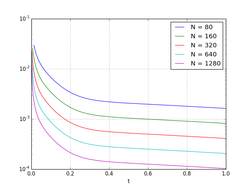
Figure 4 shows how the error varies with tnt_{n} for a sequence of solutions obtained by successively doubling NN (and hence halving Δ​t\Delta t), using a log scale. (The same spatial mesh with M=1000M=1000 subintervals was used in all cases.) Table 1 provides an alternative view of this data, listing the weighted error and its associated convergence rate,

EN=max1≤tn≤1/2⁡tnα​‖Un−u⁡(tn)‖andρN=log2⁡(EN/EN/2),E_{N}=\max_{1\leq t_{n}\leq 1/2}t_{n}^{\alpha}\|U^{n}-u(t_{n})\|\quad\text{and}\quad\rho_{N}=\log_{2}(E_{N}/E_{N/2}), (44)

so that if ENE_{N} decays like N−ρ=Δ​tρN^{-\rho}=\Delta t^{\rho} then ρ≈ρN\rho\approx\rho_{N}. As expected, ρN≈1\rho_{N}\approx 1 when α=13/16=0.8125\alpha=13/16=0.8125, but the rate deteriorates for smaller values of α\alpha.

Our analysis in Section 4 does not reveal how the constant in Theorem 4 depends on the fractional diffusion exponent ν\nu, because the proof of Lemma 9 is not constructive. The factor (1−ν)−2(1-\nu)^{-2} in the estimate of Lemma 8 raises the question of whether the DG error becomes large if ν\nu is very close to 11. We therefore investigated numerically the values of

Φ1​(ν)\displaystyle\Phi_{1}(\nu) =sup0<μ<∞maxnν≤μ−1⁡n1−2​ν​μ−2​δn​(μ),\displaystyle=\sup_{0<\mu<\infty}\max_{n^{\nu}\leq\mu^{-1}}n^{1-2\nu}\mu^{-2}\delta^{n}(\mu), (45)
Φ2​(ν)\displaystyle\Phi_{2}(\nu) =sup0<μ<∞supnν≥μ−1n1+ν​μ​δn​(μ),\displaystyle=\sup_{0<\mu<\infty}\sup_{n^{\nu}\geq\mu^{-1}}n^{1+\nu}\mu\delta^{n}(\mu),

since C=max⁡(Φ1​(ν),Φ2​(ν))C=\max\bigl(\Phi_{1}(\nu),\Phi_{2}(\nu)\bigr) is the best possible constant in Theorem 4. Figure 5 shows approximations of the graphs of Φ1\Phi_{1} and Φ2\Phi_{2}, obtained by restricting μ\mu to the discrete values 2j2^{j} for −18≤j≤20-18\leq j\leq 20, and resticting nn to the range 1≤n≤2001\leq n\leq 200. We solved (12) and (16) with u0​m=1=Um0u_{0m}=1=U^{0}_{m} and λm=μ/Δ​tν\lambda_{m}=\mu/\Delta t^{\nu} to compute δn​(μ)=Umn−um​(tn)\delta^{n}(\mu)=U^{n}_{m}-u_{m}(t_{n}). The evaluation of Φ1​(ν)\Phi_{1}(\nu) is problematic for ν\nu near zero because our values for um​(tn)u_{m}(t_{n}) are not sufficiently accurate, but it seems reasonable to conjecture that C≤1C\leq 1 for all ν\nu.

Acknowledgement

We thank Peter Brown for help with the proof of Lemma 15.

References

  • [1] C-M. Chen, F. Liu, V. Anh, and I. Turner. Numerical methods for solving a two-dimensional variable-order anomalous sub-diffusion equation. Math. Comp., 81:345–366, 2012.
  • [2] E. Cuesta, C. Lubich, and C. Palencia. Convolution quadrature time discretization of fractional diffusive-wave equations. Math. Comp., 75:673–696, 2006.
  • [3] M. Cui. Compact finite difference method for the fractional diffusion equation. J. Comput. Phys., 228:7792–7804, 2009.
  • [4] Philippe Flajolet. Singularity analysis and asymptotics of Bernoulli sums. Theoret. Comput. Sci., 215:371–381, 1999.
  • [5] Walter B. Ford. Studies on divergent series and summability, and the asymptotic developments of functions defined by Maclaurin series. Chelsea Publishing Company, New York, 1960.
  • [6] Bangti Jin, Raytcho Lazarov, and Zhi Zhou. Error estimates for a semidiscrete finite element method for fractional order parabolic equations. SIAM J. Numer. Anal., 51:445–466, 2013.
  • [7] J. Klafter and I. M. Sokolov. First steps in random walks: from tools to applications. Oxford University Press, 2011.
  • [8] T. A. M. Langlands and B. I. Henry. The accuracy and stability of an implicit solution method for the fractional diffusion equation. J. Comput. Phys., 205:719–936, 2005.
  • [9] Leonard Lewin. Polylogarithms and associated functions. North Holland, New York-Oxford, 1981.
  • [10] William McLean. Regularity of solutions to a time-fractional diffusion equation. ANZIAM Journal, 52(0), 2011.
  • [11] William McLean and Kassem Mustapha. Convergence analysis of a discontinuous Galerkin method for a fractional diffusion equation. Numer. Algor., 52:69–88, 2009.
  • [12] William McLean and Vidar Thomée. Numerical solution via Laplace transforms of a fractional order evolution equation. J. Integral Equations Appl., 22:57–94, 2010.
  • [13] William McLean, Vidar Thomée, and Lars Wahlbin. Discretization with variable time steps of an evolution equation with a positive-type memory term. J. Comput. Appl. Math., 69:49–69, 1996.
  • [14] Kassem Mustapha. An implicit finite difference time-stepping method for a sub-diffusion equation, with spatial discretization by finite elements. IMA J. Numer. Anal., 31:719–739, 2011.
  • [15] Kassem Mustapha and William McLean. Uniform convergence for a discontinuous Galerkin, time stepping method applied to a fractional diffusion equation. IMA J. Numer. Anal., 32:906–925, 2012.
  • [16] Kassem Mustapha and William McLean. Superconvergence of a discontinuous Galerkin method for fractional diffusion and wave equations. SIAM J. Numer. Anal., 51:491–515, 2013.
  • [17] J. Quintana-Murillo and S. B. Yuste. A finite difference method with non-uniform timesteps for fractional diffusion and diffusion-wave equations. Eur. Phys. J. Special Topics, 222:1987–1998, 2013.
  • [18] Vidar Thomée. Galerkin finite element methods for parabolic problems. Springer, 1997.
  • [19] David Wood. The computation of polylogarithms. Technical Report 15-92*, University of Kent, Computing Laboratory, University of Kent, Canterbury, UK, June 1992.
  • [20] Ya-nan Zhang, Zhi-zhong Sun, and Hong-lin Liao. Finite difference methods for the time fractional diffusion equation on non-uniform meshes. J. Comput. Phys., 265:195–210, 2014.
  • [21] Antoni Zygmund. Trigonometric series, Volume I. Cambridge University Press, 1959.