Implications of a PeV neutrino spectral cutoff in GRB models
Abstract
The recent discovery of extragalactic PeV neutrinos opens a new window to the exploration of cosmic-ray accelerators. The observed PeV neutrino flux is close to the Waxman-Bahcall upper bound implying that gamma-ray bursts (GRBs) may be the source of ultra-high energy cosmic rays (UHECRs). Starting with the assumption of the GRB-UHECR connection, we show using both analytical estimates and numerical simulations that the observed neutrinos can originate at the jet as a result of photopion interactions with the following implications: the neutrino spectra are predicted to have a cutoff at energy PeV; the dissipation responsible for the GRB emission and cosmic-ray acceleration takes place at distances cm from the central engine; the Thomson optical depth at the dissipation region is ; the jet carries a substantial fraction of its energy in the form of Poynting flux at the dissipation region, and has a Lorentz factor . The non-detection of PeV neutrinos coincident with GRBs will indicate that GRBs are either poor cosmic accelerators or the dissipation takes place at small optical depths in the jet.
Keywords:
neutrinos – radiation mechanisms: non-thermal – gamma ray burst: general1 Introduction
Gamma-ray bursts (GRBs) are brief flashes of gamma-rays, which are believed to form when energy is dissipated internally in an ultrarelativistic jet flow (see Piran 2004; Mészáros 2006, for reviews). The mechanisms behind the energy release and the radiative processes involved remain hotly debated. Both synchrotron emission in optically thin conditions (Katz, 1994; Rees & Meszaros, 1994; Sari et al., 1996) and dissipation at resulting in a distorted photospheric spectrum (Thompson, 1994; Mészáros & Rees, 2000; Pe’er et al., 2006; Giannios, 2006; Beloborodov, 2010; Giannios, 2012) have been explored in the literature.
GRBs are among the few known astrophysical sources powerful enough to accelerate ultra-high energy cosmic rays (UHECRs) up to eV (Waxman, 1995; Vietri, 1995). The fact that cosmic-rays (CRs) at eV are injected at a rate similar to the observed -ray production rate from GRBs makes this association interesting (Waxman & Bahcall, 1999). The coexistence of CRs and -rays in the jet results in photopion interactions and ultimately in the production of PeV neutrinos. The recent detection of IceCube neutrinos at PeV (IceCube Collaboration, 2013) with flux close to the Waxman-Bahcall (WB) upper bound strengthens the GRB-UHECR connection, although other sources, such as ultra-long GRBs, have been also suggested as good candidates (see e.g. Murase & Ioka 2013 and references therein). An intriguing discovery of IceCube is a likely break or cutoff of the neutrino spectrum at 10 PeV.
If the observed PeV neutrinos form at the GRB emitting region, then the neutrino spectrum carries important information about the conditions of the accelerator (see also Zhang & Kumar 2013). In the simplest scenario, the GRB neutrino spectrum is expected to be flat in units, reflecting the injected proton spectrum. However, this is not always the case, since the proper treatment of other effects, such as multipion production and secondary photon emission, may cause deviations from the simple flat spectrum (Baerwald et al., 2012; Asano & Meszaros, 2014; Petropoulou, 2014; Winter et al., 2014). The putative break or cutoff of the neutrino spectrum can naturally arise from the synchrotron cooling of charged pions, muons and kaons, and in this case, the location of the break strongly constrains the strength of the magnetic field at the source. This turns out to set stringent constraints on the location where dissipation takes place in the jet.
Here we assume that GRBs are the source of UHECRs and explore the implications from the presence of a break in the neutrinos. The present study is structured as follows: in §2 we exploit current information about the high-energy neutrino spectrum and derive analytical constraints for the dissipation distance in GRB flows. In §3 we complement the previous analysis by numerical calculations of GRB neutrino spectra for various parameter sets. We discuss the implications of our results on the nature of the dissipation mechanism in §4, and conclude with a summary in §5.
2 IceCube neutrinos
Currently, high-energy neutrino astronomy has produced two significant observational findings, which are summarized below:
- 1.
the detection of PeV energy neutrinos of astrophysical origin
- 2.
the all-flavour neutrino flux in the range TeV - PeV is reported to be GeV cm-2 s-1 sr-1 (IceCube Collaboration, 2013), i.e. close to the Waxman-Bahcall (WB) upper limit (Waxman & Bahcall, 1999).
Moreover, there is an indication of a spectral cutoff or softening of the neutrino spectrum between PeV (IceCube Collaboration, 2013; Aartsen et al., 2014), whose importance for the GRB physics will be discussed in the next paragraphs.
2.1 Model description
Let us consider a GRB flow of kinetic (isotropic equivalent) luminosity and bulk Lorentz factor . When the jet reaches a distance a substantial fraction of its luminosity is dissipated internally, either through shocks (e.g. Rees & Meszaros 1994) or magnetic reconnection (e.g. Spruit et al. 2001). Here, the distance is treated as a free parameter to be constrained by neutrino observations. Part of the dissipated energy results in the prompt GRB radiation , where observations indicate that is of order unity. The radiation mechanism itself still remains a subject of debate with synchrotron radiation of co-accelarated electrons (Katz, 1994; Rees & Meszaros, 1994; Chiang & Dermer, 1999) and emission from the GRB photosphere (Goodman, 1986; Mészáros & Rees, 2000; Giannios, 2006; Giannios, 2012) being usually advocated. For the purposes of the present study, however, it is sufficient to assume that the gamma-ray emission is produced at or close to the region where cosmic rays are accelerated. We refer to this region as the ‘dissipation region’. The gamma-ray compactness can be then defined as
| (1) |
while the spectrum is approximated by a Band function (Band et al., 2009) with an observed peak energy in the range 0.3-0.6 MeV for high luminosity GRBs, i.e. bursts with isotropic luminosities erg/s (Ghirlanda et al., 2005). For for the high and low energy slopes of the Band spectrum we adopt as indicative values and , respectively.
Acceleration of hadrons into a power-law form of with that extends to energies as high as eV is likely to occur both in shocks (Vietri, 1995; Waxman, 1995) and magnetic reconnection (Giannios, 2010) scenarios, thus making GRB sources potential UHECR accelerators. The high energy cutoff of the proton distribution is determined by the balance between the acceleration and radiation mechanisms that act respectively as energy gain and loss processes. The accelerated protons are subsequently injected with luminosity into the cooling zone, where we assume that they are affected only by energy loss processes. In general, the proton luminosity is a multiple of the gamma-ray luminosity, i.e. with . Here, we adopt , since values as high as 10 may lead to significant distortions of the GRB electronmagnetic (EM) spectrum because of hadronic initiated EM cascades. (Petropoulou, 2014). We further assume that in both the acceleration and cooling regions, the magnetic field and the gamma-ray photon field are the same. We note that our model treats in detail all the physical processes that take place only in the cooling region in contrast to two-zone models where the emission from both regions is taken into account (Reynoso, 2014; Winter et al., 2014).
2.2 Neutrino energy and fluence
In GRBs the local radiation field is generally strong and UHE protons may lose a significant fraction of their energy through photopion () interactions with the GRB photons (Waxman & Bahcall, 1997; Rachen & Mészáros, 1998). Here we summarize why neutrinos of PeV energy are expected from these interactions and connect the neutrino fluence to the properties of the GRB flow.
The energy threshold condition for interactions with GRB photons at the peak of the Band spectrum can be written as
| (2) |
where is the redshift of the burst and . From this point on and throughout the text we will adopt the notation in cgs units for dimensional quantities, unless stated otherwise. We also drop the “obs” qualification in order to simplify the notation. Charged pions that are produced with energy , where is the inelasticity for interactions close to the threshold, decay into lighter particles after s and give (anti)neutrinos11 1 Throughout the text we refer to both neutrinos and antineutrinos commonly as neutrinos. either directly through or indirectly through . Eventually, each neutrino carries approximately of the energy of the parent pion
| (3) |
where we assumed that the energy of the pion before it decays has not been reduced with respect to its energy at production and the subscript ‘th’ is used to remind the energy of the initial proton (see eq. (2)). Thus, the production of PeV neutrinos is a natural prediction of GRB models that advocate proton acceleration to UHE – see point (i) in §2. The energy given by eq. (3) is related to the low-energy break of the neutrino spectrum expected from GRBs (e.g. Guetta et al. 2004; Zhang & Kumar 2013). However, the presence of this break is not always clear, as it depends on the shape of the overall neutrino spectrum, which in turn is affected by other parameters, such as the optical depth for interactions (see also §3, for detailed numerical results).
The WB upper bound (Waxman & Bahcall, 1999) is an upper limit on the expected neutrino fluence from GRBs under the assumption that these are indeed the sources of UHECR acceleration and are also optically thin to interactions. Ever since the original calculation, the WB upper bound consists a benchmark value for GRB models and for the sake of completeness we briefly outline the calculation. The local injection rate of UHECRs in the range eV is erg Mpc-3 yr-1 (e.g. Cholis & Hooper 2013). For a flat injection spectrum () this corresponds to an injection rate of erg/s at the source in the range eV. This is to be compared to the local injection rate of -rays from GRBs, namely erg Mpc-3 yr-1, as found by e.g. integrating the GRB lunimosity function of Wanderman & Piran (2010). If denotes the fraction of the energy lost by protons through interactions, then the resulting all-flavour neutrino flux is given by (Cholis & Hooper, 2013)
| (4) |
where accounts for the redshift evolution of the source, which is assumed to track the star formation rate (e.g.Waxman 2013). Assuming that all the observed neutrino flux of GeV cm-2 sr-1 s-1 originates from typical GRBs, eq. (4) implies that .
One can envision cases with or , which, however, we do not favour. On the one hand, one could think of a scenario where GRB jets inject more energy to non-thermal hadrons than to gamma-rays, i.e. . In this case, the observed neutrino flux would imply . However, as we will show in §3, the resulting neutrino spectra for cannot account for the observed spectral shape in the range 100 TeV-2 PeV. In addition to this, cases with may prove to be problematic for other reasons, such as the hadronic dominance in the GRB photon spectra (Asano & Meszaros, 2014; Petropoulou, 2014). On the other hand, optically thick (to interactions) scenarios where are most likely overuled because of two reasons: even if , the produced neutrino flux exceeds the observed value and in such conditions cosmic ray acceleration to eV is unlikely to take place (see next section).
The previous discussion relies on the assumption that all the IceCube neutrino flux originates from typical GRB sources. If only a fraction of the PeV neutrino flux turns out to come from GRBs, one can only set an upper limit to . In the following, we focus on the limit but explore other values for as well.
2.3 Constraints on the dissipation region
We use the following basic arguments in order to put constraints on the distance of the dissipation region:
- •
the observed neutrino flux implies that ,
- •
the acceleration of protons to UHE eV should not be hampered by cooling processes in the acceleration region.
We start with the first argument and express the fraction in terms of GRB observables, such as the gamma-ray luminosity and peak energy, and of the two main unknowns in GRB models, namely the bulk Lorentz factor and the dissipation distance. The energy loss timescale of protons because of interactions with gamma-ray photons is found to be constant (Waxman & Bahcall, 1997; Petropoulou, 2014) for protons having energy above (see eq. (2)). This can be written as
| (5) |
where . The ratio is usually defined as and expresses the fraction of energy lost by protons to pions within the expansion time:
| (6) |
where we also used eq. (1). This ratio can be directly related to the neutrino flux as long as the synchrotron cooling timescale is larger than , which is indeed the case for protons that are responsible for the PeV neutrino emission. By normalizing to the value implied by the observed neutrino fluence, namely , we define a characteristic radius as
| (7) |
This serves as an upper limit for the dissipation distance, since for the efficiency of process drops significantly and (see §3, for the implications on the neutrino spectra).
The second argument can be used in order to place a lower limit on the dissipation distance. Here, we assume that the proton acceleration process operates close to the Bohm diffusion limit, since such high acceleration rates can be achieved both in shocks and magnetic reconnection regions (Giannios, 2010). In this case, the acceleration timescale is , where is the Lorentz factor of the proton and is the magnetic field strength in the rest frame of the jet, which at a distance from the central engine is given by
| (8) |
In the above, denotes the ratio of the Poynting luminosity to the jet kinetic luminosity22 2 The total jet luminosity is then simply the sum of Poynting and kinetic luminosities.. The acceleration process competes with energy loss processes, such as radiative and adiabatic cooling, and the balance between the two defines a saturation (maximum) energy for the particles.
Radiative losses include proton synchrotron radiation and interactions. Proton-proton (pp) collisions also result in energy losses for cosmic ray protons but are not important for the parameter regime relevant to this study. Given that the cross section for inelastic pp scattering of a cosmic ray proton with one of low energy is cm2, (The Atlas Collaboration et al., 2011), inelastic collisions become important at Thomson optical depths of the flow larger than ; for the definition of see below.
The synchrotron cooling timescale for a proton , where . Demanding and using eq. (8) we find that the dissipation should occur at distances larger than
| (9) |
in order for the acceleration process to saturate at eV. The above apply also to interactions that may overtake synchrotron losses for high gamma-ray compactnesses. Using eq. (5) we find that the condition is equivalent to , where the latter is given by
| (10) |
Combining eqs. (9) and (10) we find that synchrotron losses dominate over losses, unless exceeds
| (11) |
Finally, the acceleration mechanism competes with the expansion timescale of the flow. However, the condition sets a weak constraint on the bulk Lorentz factor, i.e. and we will not consider it any further.

Combining all the above we can constrain the distance of the dissipation region between and . This is examplified in Fig. 1 for erg/s, , . In addition to the above constraints we overplotted (blue thick line) for comparison reasons the ‘photospheric’ radius (), i.e. the locus of points on the plane that correspond to . Since the optical depth of the jet as function of distance is (e.g. Mészáros & Rees 2000; Giannios 2012) the location of the Thomson photosphere can be written as
| (12) |
Finally, the color coding indicates the predicted spectral cutoff energy of the observed neutrino spectrum because of synchrotron pion cooling. This characteristic neutrino energy, which we will call ‘break’ energy from this point on, is given by
| (13) |
For the above derivation we used eqs. (7) and (8) and the fact that where . Here is the Lorentz factor of a pion that cools because of synchrotron radiation before it decays, i.e.
| (14) |
where . Figure 1 reveals a few things about the GRB source that are worth commenting on:
- •
the dissipation takes place close to the Thomson photosphere;
- •
the constraint imposed by the observed neutrino fluence () sets an upper limit on the observed spectral cutoff of the neutrino spectrum, which is PeV as indicated by the color bar;
- •
the bulk Lorentz factor is less constrained as it ranges between 100 and 1000.
If, however, GRBs prove to be only subdominant sources of the observed PeV neutrino flux, Fig. 1 should be interpreted as follows: the dissipation region is placed at larger distances from the central engine (white colored region above the line), the neutrino spectrum extends at energies above 10 PeV, while the Lorentz factor still remains the less constrained parameter.

2.4 Dependence on
At the moment there is only evidence for a spectral cutoff of the neutrino spectrum between 2 and 10 PeV. If this is confirmed, then the constraints shown in Fig. 1 allow us to build a consistent picture where the dissipation of energy occurs at such distances that favor both UHECR acceleration and neutrino emission with flux values close to the observed one. However, a future detection of neutrino events with a flat spectrum (in ) units extending above 10 PeV would have some interesting implications which we will discuss in §3 with detailed examples.
Here we keep the break energy of the neutrino spectrum as a free parameter and we express the various quantities introduced in §2 in terms of PeV. For the magnetic field strength we find
| (15) |
where we used that and eq. (14). Combining eqs. (8) and (15) the dissipation distance is written as
| (16) |
Thus, if the high energy neutrino spectrum extends above a few PeV, the dissipation region should be placed at larger distances (), simply because the magnetic field is smaller further out from the central engine. This is also reflected at the inverse proportional dependence of on :
| (17) |
where we used the definition and eq. (16). Finally, the gamma-ray compactness is written as
| (18) |
where we used eqs. (1) and (16). Large values of correspond to a small gamma-ray compactness, which further implies a decrease in the neutrino flux, given a fixed value of the ratio – for the relation between and the neutrino production efficiency see Petropoulou (2014). Finally, by equating and using the expression (15) for the magnetic field, we estimate the maximum energy of a proton, if limited by synchrotron losses, to be:
| (19) |
If proton acceleration is saturated by interactions we find
| (20) |
where we used . Thus, the maximum proton energy is typically determined by the balance between the acceleration and synchrotron loss rates, unless .
The magnetization of the burst, which is one of the basic unknowns in GRB models, was kept fixed up to this point. Here, we investigate the role of on the constraints presented in Fig. 1. For this, we plot the dissipation distance given by eq. (16) as a function of for and – see Fig.2. For each value of we show the expected for two indicative values of the neutrino spectral break energy, i.e. and 6, while is shown with thick red line. The dissipation region for is placed well inside the GRB photosphere, where other physical processes, such as pp collisions may prevent UHECR acceleration in the first place. Note that if , the dissipation may still be located at regions with provided that , though in that case acceleration of protons up to eV is unlikely (see eq. (20). The verification of a spectral cutoff in the IceCube spectrum between 2 and 10 PeV will, thus, favour substantially magnetized GRB flows with .
3 Numerical approach
In the previous section we derived strong constraints on the location of the dissipation region using analytical arguments. The detailed numerical calculations of neutrino spectra reported here fully support this analysis and provide some additional constraints, which come from the fact that the observed neutrino spectrum is modeled as with in the 60 TeV-3 PeV energy range (Aartsen et al., 2014). First, we present neutrino spectra obtained for a single GRB located at a fiducial redshift . Then, we calculate the diffuse GRB neutrino emission and compare our results against the IceCube detection.
| # | (PeV) | (G) | (cm) | ||||
| 1 | 200 | 50 | 17 | 0.009 | |||
| 2 | 300 | 50 | 11.3 | 0.006 | |||
| 3 | 500 | 50 | 7 | 0.004 | |||
| 4 | 1000 | 50 | 3.4 | 0.002 | |||
| 5 | 200 | 10 | 85 | 0.05 | |||
| 6 | 300 | 10 | 57 | 0.03 | |||
| 7 | 500 | 10 | 34 | 0.02 | |||
| 8 | 1000 | 10 | 17 | 0.01 | |||
| 9 | 200 | 3 | 300 | 0.2 | |||
| 10 | 300 | 3 | 170 | 0.1 | |||
| 11 | 500 | 3 | 113 | 0.06 | |||
| 12 | 1000 | 3 | 57 | 0.03 | |||
|
|


3.1 Numerical code
For this calculation we employed a kinetic equation approach, as described in Dimitrakoudis et al. (2012)– henceforth, DMPR12. The production and loss rates of five stable particle species (protons, neutrons, electrons (including positrons), photons and neutrinos (of all flavours)) are tracked self-consistently with five time-dependent equations. In addition to the processes outlined in Petropoulou (2014), we now also include the effects of kaon, pion, and muon synchrotron losses, albeit in a way that does not require the use of additional kinetic equations. Pion, charged and neutral ( and ) kaon production rates from photo-meson interactions have been computed by the SOPHIA event generator (Mücke et al., 2000). For each particle energy, we calculate the energy lost to synchrotron radiation before it decays. The remainder of that energy is then instantaneously transferred to the particle’s decay products, whose yields have also been computed by the SOPHIA event generator. Since the secondary particles from kaon decay include pions, we first calculate charged kaon decay and then charged pion decay. Finally, the same process is applied to the resulting muons. The photons, electrons, and neutrinos resulting from kaon, pion, and muon decay are added as production rates to their respective kinetic equations, as are the photons from kaon, pion, and muon synchrotron radiation. Neutral kaons ( and ) and pions () are, as in DMPR12, assumed to decay instantaneously, therefore directly contributing their decay products to the kinetic equations.
Summarizing, the numerical code as presented in DMPR12 but augmented in a way to include pion, muon and kaon synchrotron cooling, is comparable to other Monte Carlo (MC) codes at least in the particle physics part (e.g. Asano et al. 2009; Hümmer et al. 2010; Baerwald et al. 2011; Murase et al. 2012; Baerwald et al. 2012), while it comes with the advantage of treating time-dependent problems self-consistently (see e.g. Mastichiadis et al. 2005; Petropoulou & Mastichiadis 2012). A detailed comparison of the augmented DMPR12 code with the NeuCosmA (Baerwald et al., 2012) MC code can be found in Appendix A. In the same section, we further demonstrate using the DMPR12 code the effects of other processes, such as neutron photopion interactions and injection of secondaries in the emission region, on the neutrino spectra.
3.2 Numerical results
In total we performed twelve simulations for different values of and , while we kept fixed erg/s, and . All the parameter values used in our simulations are summarized in Table 1.
Indicative neutrino spectra obtained from a single GRB at redshift are shown in Fig. 3. Here, we plot the sum of the electron and muon neutrino and antineutrino fluxes befor flavour mixing. For GRBs at cosmological distances, however, the initial ratio becomes because of neutrino oscillations (Learned & Pakvasa, 1995). In this context, the neutrino spectra obtained from our simulations are equivalent to the all-flavour observed neutrino spectra. The contribution of muon, charged pion and kaon decays to the total neutrino spectrum can be identified by the three ‘bumps’ from low to high energies in agreement to previous studies (e.g. Baerwald et al. 2011) – see also Appendix A for more details.
Panel (a) demonstrates the effect that has on the neutrino spectral shape for cases with the same or equivalently (see eq. (13)). Higher values of lead to lower neutrino fluxes and harder spectra33 3 his effect becomes more prominent as the source becomes more optically thin to interactions, i.e. for lower . . The increase of within each group of cases with the same is equivalent to stronger magnetic fields and lower values of the gamma-ray compactness. Higher magnetic fields cause more severe synchrotron losses to charged pions, kaons and muons, thus leading to a decrease of the neutrino flux. Moreover, the neutrino production efficiency drops as the source becomes less compact in gamma-rays (see also Petropoulou 2014), which also reduces the flux, given that all other parameters are kept the same. In all cases, the low-energy bump of the neutrino spectrum moves to higher values for larger (see also eq. (3)). For example, the spectrum peaks at PeV for PeV and . However, there is a qualitative change seen in the neutrino specta caused mainly by the increase of the magnetic field. For high enough magnetic fields, e.g. MG, we find that the second bump of the spectrum, which is related to the direct pion decay, carries most of the neutrino luminosity (dotted line in panel (a) of Fig. 3). This result is also in agreement with the study of Baerwald et al. (2012) (see Fig. 5 therein). Summarizing, models that result in hard neutrino spectra, cannot account for the sub-PeV neutrino emission.
Cases with the same value of but different cutoff energies are shown in panel (b). The neutrino flux decreases as the spectral break moves to higher energies, which is the result of both decreasing and . A future detection of neutrinos above PeV will, therefore, point towards large dissipation distances and low Lorentz factors, e.g. , in order to achieve both the flat spectral shape and the observed flux.
Having explained the basic features of the single burst neutrino emission, we proceed with the calculation of the diffuse neutrino flux. For this, we used as a typical duration for long GRBs s (Goldstein et al., 2012; Gruber et al., 2014) and assumed that the GRB rate follows the star formation (SF) rate. In particular, we adopted the second SF model by Porciani & Madau (2001) and for the local GRB rate we used the value derived by Wanderman & Piran (2010), i.e. Gpc-3 yr-1. Thus, the GRB rate as a function of redshift is written as
| (21) |
We obtain first from the numerical simulations the neutrino fluence as measured in the rest frame of the galaxy () and then we calculate the diffuse neutrino flux in GeV cm-2 s-1 sr-1 (see also Murase & Nagataki 2006; Cholis & Hooper 2013) as
| (22) |
where km Mpc-1 s-1, , and for a flat universe.
Our results are presented in Figs. 4(a)-4(c) along with the flux value measured by IceCube GeV cm-2 s-1 sr-1. The upper limit of ANITA II (Gorham et al., 2010), the upper limit on -neutrino flux by Pierre Auger (Abraham et al., 2008), and the expected 3-year sensitivity of ARA (Ara Collaboration et al., 2012) are also shown.
|
|


Cases 1-4 with spectral cutoff at PeV (panel (a)) cannot account for the observed neutrino spectra. These are obtained for relatively large values of where the efficiency of pion production is small – here, . One could argue that for the neutrino flux would be close to the observed value. Even in this case the hard spectrum below the PeV energy range would contradict the observations, except for . However, given that GRBs are expected to come from jets with , the suggestion that all bursts should be accompanied by slow jets requires fine tuning. Cases 5-7 and 9-12 predict fluxes close44 4 The model derived fluxes lie close but still below the low observational error bar. We argue, however, that these cases can account for the IceCube observations, since a different model for the SF rate or , would result in spectra with higher fluxes and the adequate shape. to the the IceCube measurements and result in soft or even flat spectra, see e.g. Cases 5 and 12, respectively. As long as GRBs are the only sources contributing to the observed PeV flux, Cases 5-7, 9-12 favour scenarios with relatively small dissipation distances (), moderate-to-low values of , and strong magnetic fields ( G) – see Table 1. If, however, the IceCube PeV neutrino-GRB connection is disfavoured (see e.g. Hümmer et al. 2012; He et al. 2012; Liu & Wang 2013), would indicate that GRBs are poor cosmic ray accelerators or, alternatively, large-distance dissipation scenarios would be more appropriate making Cases 1-4 more relevant.
All neutrino spectra shown in Figs. 4 (a)-(c) extend up to EeV. We find that this energy range is dominated either by the exponential cutoff of the direct pion decay bump (Cases 1-4) or by the kaon-decay bump (Cases 5-12). Because of this, the expected GRB neutrino flux at EeV is only a small fraction () of the IceCube value. Yet, the value GeV cm-2 s-1 sr-1 is close to the expected sensitivity limit of next generation experiments, such as ARA (Ara Collaboration et al., 2012), and in this respect, Cases 1-4 are promissing. A future detection of EeV neutrinos cannot be used, in principle, to distinguish between different GRB models mainly because of the contribution of cosmogenic (GZK) neutrinos at this particular energy range (Beresinsky & Zatsepin, 1969; Stecker, 1973). To illustrate this, we plotted the model of Yüksel & Kistler (2007) for GZK neutrinos (blue line), which predicts a higher flux at this energy range than other GZK models (see e.g. Fig. 29 on Ara Collaboration et al. 2012). Although both GRBs and GZK neutrinos may contribute to this energy range, their spectra are radically different, namely soft and hard respectively (see e.g. panel (a) in Fig. 4). This may prove to be a strong diagnostic tool, if the sensitivity of future experiments allows spectral construction. We note also that radio-loud blazars may have a non-negligible contribution to this energy range (Murase et al., 2014). In any case, a discrimation between the various contributions seems to be necessary.
3.3 The revised plane

The numerical analysis of the previous section acts complementary to the analytical approach presented in §2. Here, we use this additional information in order to place even stronger constraints on the dissipation distance. The revised plane is shown in Fig. 5. The characteristic radii and are plotted with solid and dashed lines, respectively, while the parameter sets used in §3.2 are shown as symbols. In particular, sets that correspond to PeV (), 10 PeV ( ) and 3 PeV () are shown with triangles, squares and circles, respectively. We use filled symbols, only if the calculated neutrino spectra can account for the current IceCube observations (see panels (a)-(c) in Fig. 3); open symbols are used, otherwise. The final allowed parameter space (grey colored region) is truncated compared to the one shown in Fig. 1, as the region for is now excluded. We caution the reader that if the GRB-PeV neutrino connection is disproved, then the region above the grey colored one should be considered as allowable, thus favoring long-distance dissipation scenarios.
4 Discussion
The characteristics (fluence and shape) of the high-energy neutrino spectrum expected from GRBs depends sensitively on the compactness of the dissipation region and, for this reason, they can be used as a probe. In §3 we showed how the fluence and the indication of a spectral cutoff at a few PeV place the dissipation region fairly close to the Thomson photosphere (see also Murase 2008). Additional information from the neutrino spectra favors jets with bulk Lorenz factor and, hence, exclude part of the parameter space. Interestingly, independent studies on spectral formation close and above the GRB photosphere because of continuous energy dissipation seem promising for the GRB emission itself (e.g. Giannios 2012). What causes therefore the dissipation and UHECR acceleration at in the jet?
If the jet contains a substantial neutron component, energy dissipation through neutron-proton collisions is possible. The dissipation peaks at where the decoupling of the neutron and proton fluids takes place, and continues further out in the flow at smaller optical depths (e.g. Beloborodov 2010; Vurm et al. 2011; Koers & Giannios 2007). In this picture, most of the collisions take place at mildly relativistic speeds throughout the volume of the jet, heating the flow. It is not obvious, however, how CRs can be accelerated to ultra-high energies in such scenario.
For high values of , the dissipation distance that we infer does not differ much from the radius of the progenitor cm, thus making recollimation shocks a likely culprit for the dissipation (Lazzati et al., 2007). However, it is not clear whether the jet, after crossing the stellar surface, can reach a terminal of several hundreds by a distance of cm. This depends on several parameters, such as the magnetization of the flow and the external pressure (Sapountzis & Vlahakis, 2013). The Lorentz factor achieved during the first acceleration phase, which takes place inside the star, plays also a crucial role (Komissarov et al., 2010). Moreover, even if a satisfactory dissipation mechanism operated at these small distances, the resulting neutrino spectra for would be too hard to explain the observed spectrum.
Our analysis showed that GRB neutrino spectra are compatible with the IceCube observations for and cm. In this range, both internal shocks and magnetic reconnection can be invoked as possible dissipation mechanisms. Internal shocks occur at distances cm, where is the observed variability timescale. Interestingly, the same scaling applies also to scenarios of magnetic reconnection. It can be shown (see e.g. Drenkhahn & Spruit 2002) that in a strongly magnetized jet with magnetic field reversals on a scale the reconnection distance is cm, where we have assumed that the GRB central engine contains magnetic field reversals on a scale cm and that the reconnection takes place at the speed . Here, we used a conservative value for the reconnection rate. Magnetic reconnection, however, may proceed at a fairly slow rate in the collisional region and speed up at because of a switch from collisional to collisionless conditions (McKinney & Uzdensky, 2012). Although in both cases a fine tuning appears to be required so that the dissipation takes place preferentially at the inferred distance, magnetic reconnection remains a viable mechanism for Poynting-flux dominated jets, whereas internal shocks prove to be problematic (e.g. Sironi & Spitkovsky 2009). With the current IceCube data our analysis points, indeed, towards strongly magnetized jets with G. Future verification of a spectral cutoff PeV will exclude GRB models with low magnetization, e.g. , as these require .
If magnetic reconnection in Poynting-flux dominated jets proves to be the dissipation mechanism in GRBs, then the problem of proton acceleration in reconnection layers becomes relevant. Here, we used only rough estimates of the acceleration and energy loss timescales and showed that UHECR can be achieved at distances close to the GRB photosphere. Recent particle-in-cell (PIC) simulations have shown that relativistic reconnection can produce non-thermal electrons with hard power-law spectra () in regions with high magnetization. The electron energy is found to increase linearly with time close to the Bohm diffusion limit (Sironi & Spitkovsky, 2014). Although there is no definite answer to the problem of proton (ion) acceleration in relativistic reconnection, there are indications that the acceleration process in pair plasmas and electron-ion plasmas shares many features, such as the acceleration rate and the power-law slope (private communication with Dr. L. Sironi).
The above implications on the physical conditions of the GRB emission site hold as long as the assumption of the ‘typical’ GRBs being the sources of PeV neutrinos is still valid. However, the non-detection of individual GRBs by IceCube so far starts putting severe constraints on this possibility. For example, by considering the existing IceCube limit on the neutrino flux of triggered GRBs, this GRB population can only account for a flux of a few GeV cm-2 s-1 sr-1 (e.g. Liu & Wang 2013). In this case, our analysis should be translated as follows: either ‘typical’ GRBs cannot accelerate CRs to UHE or the physical conditions are such as to suppress pion and neutrino production, i.e. the grey-colored region in Fig. 5 would be not allowed and the dissipation distance would have to be placed further out to the flow where (see also Zhang & Yan 2011). The PeV neutrino flux could still originate from GRBs, but from the low-luminosity class (e.g. Cholis & Hooper 2013; Murase & Ioka 2013), as their rate is uncertain and they would not violate the stacking limits derived by triggered GRBs (Abbasi et al., 2010; Abbasi et al., 2011; Abbasi et al., 2012).
5 Conclusions
We explored the implications of the recent PeV astrophysical neutrino detection with IceCube on the properties of the GRB flow. The prompt gamma-ray emission provide the targets for photopion interactions of protons having energy eV. These lead to the creation of high-energy pions that subsequently decay into PeV neutrinos. In principle, the GRB neutrino spectrum is predicted to have two breaks: the (sub)PeV break is related to the energy threshold for pion production with photons from the peak of the GRB spectrum, whereas the second break () is related to synchrotron cooling of the parent pions. The latter depends on the comoving magnetic field strength as G.
IceCube has presented the first evidence for a cutoff in the neutrino spectrum at energies PeV. Given that GRB jets are expected to have , the field strength at the emission region has to be G. This inference places the dissipation region at a fairly compact location in the jet. We estimated the fraction of proton energy lost to pion production within the expansion time () at such distances and found , i.e. close to the value inferred from the IceCube detection. Thus, an observed cutoff of the neutrino spectrum at several PeV actually implies that the neutrino flux is close to the Waxman-Bahcall (WB) upper limit. We elaborate on this remark using detailed numerical simulations. In general, our numerical results confirmed the connection between and the expected neutrino fluence, except for cases with high Lorentz factors () where the neutrino spectra are too hard with a large curvature.
Despite the compactness of the dissipation region, protons can be accelerated to energies up to eV provided that the magnetic field in the jet is not very weak . On the one hand, there is evidence that the composition of UHECRs changes from light (protons) to heavy (Fe) for energies eV(Pierre Auger Collaboration et al., 2011), and GRB jets may be rich in heavy nuclei, too (Metzger et al., 2011). On the other hand, observations at eV indicate a light composition for UHECRs. Moreover, in many scenarios for UHECR acceleration, protons dominate the composition at PeV energies, and since these are responsible for the PeV neutrino production, our main conclusions are left unchanged.
Summarizing, the verification of a cutoff of the neutrino spectrum at energies below a few Pev has two profound implications for the GRB flow. First, the jet carries a substantial fraction of its luminosity in the form of Poynting flux and the emission region is strongly magnetized with comoving magnetic fields of MG. Second, the dissipation of energy takes place close to the Thomson photosphere at distances cm. Unambiguous proof of the connection between GRBs and PeV neutrinos can come from the simultaneous detection of both high-energy signatures. So far, however, no such detection has taken place, placing increasingly strict limits on the possible contribution of classical GRB to the ambient neutrino flux. Such a detection will not only reveal a strong candidate source of UHECRs but will also be a unique probe of where in the jet the dissipation takes place.
Acknowledgements
We would like to thank the anonymous referee for helping improving the manuscript. We thank also Prof. A. Mastichiadis, Prof. Kohta Murase, Prof. W. Winter and Dr. X. Y. Wang for useful discussions. Support for this work was provided by NASA through Einstein Postdoctoral Fellowship grant number PF3 140113 awarded by the Chandra X-ray Center, which is operated by the Smithsonian Astrophysical Observatory for NASA under contract NAS8-03060. DG acknowledges support from the Fermi 6 cycle grant number 61122.
References
- Aartsen et al. (2014) Aartsen M. G. et al., 2014, ArXiv e-prints
- Abbasi et al. (2012) Abbasi R. et al., 2012, Nature, 484, 351
- Abbasi et al. (2010) Abbasi R. et al., 2010, ApJ, 710, 346
- Abbasi et al. (2011) Abbasi R. et al., 2011, Physical Review Letters, 106, 141101
- Abraham et al. (2008) Abraham J. et al., 2008, Physical Review Letters, 100, 211101
- Ara Collaboration et al. (2012) Ara Collaboration et al., 2012, Astroparticle Physics, 35, 457
- Asano et al. (2009) Asano K., Inoue S., Mészáros P., 2009, ApJ, 699, 953
- Asano & Meszaros (2014) Asano K., Meszaros P., 2014, ArXiv e-prints
- Baerwald et al. (2011) Baerwald P., Hümmer S., Winter W., 2011, PhysRevD, 83, 067303
- Baerwald et al. (2012) Baerwald P., Hümmer S., Winter W., 2012, Astroparticle Physics, 35, 508
- Band et al. (2009) Band D. L. et al., 2009, ApJ, 701, 1673
- Beloborodov (2010) Beloborodov A. M., 2010, MNRAS, 407, 1033
- Beresinsky & Zatsepin (1969) Beresinsky V. S., Zatsepin G. T., 1969, Physics Letters B, 28, 423
- Beringer et al. (2012) Beringer J. et al., 2012, Physical Review D, 86, 010001
- Chiang & Dermer (1999) Chiang J., Dermer C. D., 1999, ApJ, 512, 699
- Cholis & Hooper (2013) Cholis I., Hooper D., 2013, JCAP, 6, 30
- Dimitrakoudis et al. (2012) Dimitrakoudis S., Mastichiadis A., Protheroe R. J., Reimer A., 2012, A&A, 546, A120
- Drenkhahn & Spruit (2002) Drenkhahn G., Spruit H. C., 2002, A&A, 391, 1141
- Ghirlanda et al. (2005) Ghirlanda G., Ghisellini G., Firmani C., Celotti A., Bosnjak Z., 2005, MNRAS, 360, L45
- Giannios (2006) Giannios D., 2006, A&A, 457, 763
- Giannios (2010) Giannios D., 2010, MNRAS, 408, L46
- Giannios (2012) Giannios D., 2012, MNRAS, 422, 3092
- Goldstein et al. (2012) Goldstein A. et al., 2012, Astrophysical Journal Suppl. Ser., 199, 19
- Goodman (1986) Goodman J., 1986, ApJL, 308, L47
- Gorham et al. (2010) Gorham P. W. et al., 2010, PhysRevD, 82, 022004
- Gruber et al. (2014) Gruber D. et al., 2014, Astrophysical Journal Suppl. Ser., 211, 12
- Guetta et al. (2004) Guetta D., Hooper D., Alvarez-Mun˜Iz J., Halzen F., Reuveni E., 2004, Astroparticle Physics, 20, 429
- He et al. (2012) He H.-N., Liu R.-Y., Wang X.-Y., Nagataki S., Murase K., Dai Z.-G., 2012, ApJ, 752, 29
- Hümmer et al. (2012) Hümmer S., Baerwald P., Winter W., 2012, Physical Review Letters, 108, 231101
- Hümmer et al. (2010) Hümmer S., Rüger M., Spanier F., Winter W., 2010, ApJ, 721, 630
- IceCube Collaboration (2013) IceCube Collaboration, 2013, Science, 342
- Katz (1994) Katz J. I., 1994, ApJL, 432, L107
- Koers & Giannios (2007) Koers H. B. J., Giannios D., 2007, A&A, 471, 395
- Komissarov et al. (2010) Komissarov S. S., Vlahakis N., Königl A., 2010, MNRAS, 407, 17
- Lazzati et al. (2007) Lazzati D., Morsony B. J., Begelman M. C., 2007, Royal Society of London Philosophical Transactions Series A, 365, 1141
- Learned & Pakvasa (1995) Learned J. G., Pakvasa S., 1995, Astroparticle Physics, 3, 267
- Lipari et al. (2007) Lipari P., Lusignoli M., Meloni D., 2007, Physical Review D, 75, 123005
- Liu & Wang (2013) Liu R.-Y., Wang X.-Y., 2013, ApJ, 766, 73
- Mastichiadis et al. (2005) Mastichiadis A., Protheroe R. J., Kirk J. G., 2005, A&A, 433, 765
- McKinney & Uzdensky (2012) McKinney J. C., Uzdensky D. A., 2012, MNRAS, 419, 573
- Mészáros (2006) Mészáros P., 2006, Reports on Progress in Physics, 69, 2259
- Mészáros & Rees (2000) Mészáros P., Rees M. J., 2000, ApJ, 530, 292
- Metzger et al. (2011) Metzger B. D., Giannios D., Horiuchi S., 2011, MNRAS, 415, 2495
- Mücke et al. (2000) Mücke A., Engel R., Rachen J. P., Protheroe R. J., Stanev T., 2000, Computer Physics Communications, 124, 290
- Murase (2008) Murase K., 2008, PhysRevD, 78, 101302
- Murase et al. (2012) Murase K., Asano K., Terasawa T., Mészáros P., 2012, ApJ, 746, 164
- Murase et al. (2014) Murase K., Inoue Y., Dermer C. D., 2014, ArXiv e-prints
- Murase & Ioka (2013) Murase K., Ioka K., 2013, Physical Review Letters, 111, 121102
- Murase & Nagataki (2006) Murase K., Nagataki S., 2006, PhysRevD, 73, 063002
- Pe’er et al. (2006) Pe’er A., Mészáros P., Rees M. J., 2006, ApJ, 642, 995
- Petropoulou (2014) Petropoulou M., 2014, accepted by MNRAS
- Petropoulou & Mastichiadis (2012) Petropoulou M., Mastichiadis A., 2012, MNRAS, 421, 2325
- Pierre Auger Collaboration et al. (2011) Pierre Auger Collaboration et al., 2011, JCAP, 6, 22
- Piran (2004) Piran T., 2004, Reviews of Modern Physics, 76, 1143
- Porciani & Madau (2001) Porciani C., Madau P., 2001, ApJ, 548, 522
- Rachen & Mészáros (1998) Rachen J. P., Mészáros P., 1998, PhysRevD, 58, 123005
- Rees & Meszaros (1994) Rees M. J., Meszaros P., 1994, ApJL, 430, L93
- Reynoso (2014) Reynoso M. M., 2014, ArXiv e-prints
- Sapountzis & Vlahakis (2013) Sapountzis K., Vlahakis N., 2013, MNRAS, 434, 1779
- Sari et al. (1996) Sari R., Narayan R., Piran T., 1996, ApJ, 473, 204
- Sironi & Spitkovsky (2009) Sironi L., Spitkovsky A., 2009, ApJ, 698, 1523
- Sironi & Spitkovsky (2014) Sironi L., Spitkovsky A., 2014, ApJL, 783, L21
- Spruit et al. (2001) Spruit H. C., Daigne F., Drenkhahn G., 2001, A&A, 369, 694
- Stecker (1973) Stecker F. W., 1973, Ap&SS, 20, 47
- The Atlas Collaboration et al. (2011) The Atlas Collaboration et al., 2011, Nature Communications, 2
- Thompson (1994) Thompson C., 1994, MNRAS, 270, 480
- Vietri (1995) Vietri M., 1995, ApJ, 453, 883
- Vurm et al. (2011) Vurm I., Beloborodov A. M., Poutanen J., 2011, ApJ, 738, 77
- Wanderman & Piran (2010) Wanderman D., Piran T., 2010, MNRAS, 406, 1944
- Waxman (1995) Waxman E., 1995, ApJL, 452, L1
- Waxman (2013) Waxman E., 2013, ArXiv e-prints
- Waxman & Bahcall (1997) Waxman E., Bahcall J., 1997, Physical Review Letters, 78, 2292
- Waxman & Bahcall (1999) Waxman E., Bahcall J., 1999, PhysRevD, 59, 023002
- Winter et al. (2014) Winter W., Becker Tjus J., Klein S. R., 2014, ArXiv e-prints
- Yüksel & Kistler (2007) Yüksel H., Kistler M. D., 2007, PhysRevD, 75, 083004
- Zhang & Kumar (2013) Zhang B., Kumar P., 2013, Physical Review Letters, 110, 121101
- Zhang & Yan (2011) Zhang B., Yan H., 2011, ApJ, 726, 90
Appendix A Comparison between the DMPR12 and NeuCosmA codes
The GRB neutrino spectrum may deviate from the often adopted Waxman-Bahcall trapezoidal spectral shape (e.g. Abbasi et al. 2010). A more detailed treatment of the physical processes involved, such as inclusion of the multipion production channels, may lead to more complex shapes (e.g. Baerwald et al. 2011).
Here we attempt a detailed comparison between the neutrino spectra obtained with our numerical code (DMPR12), which combines the physics of the SOPHIA code with the kinetic equation approach, and those obtained with the Monte Carlo (MC) code NeuCosmA (Hümmer et al., 2010). For the comparison we chose the electron and muon neutrino spectra shown in Fig. 18 of Baerwald et al. (2012) – henceforth BHW12. These are calculated at the rest frame of the emission region for G, , , and . The GRB spectrum is modeled having a break at keV and extending from eV to , with photon indices below and above the peak and , respectively.
In order to use the same assumptions as in BHW12, we modified the DMPR12 code accordingly by neglecting the:
- 1.
neutron photopion production
- 2.
modification of the GRB photon spectrum due to the emission of secondaries, e.g. gamma-rays from decay
- 3.
modification of the low-energy part of GRB spectrum because of synchrotron self-absorption
- 4.
modification of the high-energy ( MeV) part of the GRB spectrum due to photon-photon absorption
- 5.
modification of the injected proton distribution due to cooling.
The size of the emission region as well as the injection compactness of protons and GRB photons are necessary input quantities for the DMPR12 code, which is a PDE solver, in contrast to MC codes. Given that the above quantities are not defined in BHW12, we use the fiducial values cm, and , and normalize a posteriori the resulting neutrino spectra with respect to those in Fig. 18 of BHW12.
The electron and muon neutrino spectra are shown in the top and bottom panels of Fig. 6, respectively. The neutrino spectra of BHW12 when synchrotron losses of pions, muons and kaons are taken into account are plotted with open circles, whereas filled circles correspond the no loss case. Our results are overplotted with solid (no losses) and dashed (with losses) lines. The neutrino spectra obtained by neglecting the production are also shown with dotted lines.
In the case where the losses of secondaries are not taken into account, we find a good agreement between the two codes except for a small deviation at the high-energy part of the spectra. This is caused by a difference at the high-energy cutoff of the proton distribution, which in our case is abrupt, whereas in BHW12 is assumed to be exponential. When synchrotron losses of secondaries are taken into account, we find that the electron and muon neutrino spectra calculated with the DMPR12 code are in agreement with those of BHW12 at energies GeV and GeV, respectively. Above these energies, where the neutrino spectrum is mainly determined by the kaon decays, we find deviations from the BHW12 results, which become prominent mainly in the electron neutrino spectra. The main reason for these differences is that the DMPR12 code takes into account the decay of all types of kaons, such as the short-lived () and long-lived () neutral kaons, whereas BHW12 considered only the leading mode of production.
Inclusion of the decays leads not only to an absolute inrease of the electron and muon neutrino fluxes but also to a relative increase of the electron to muon neutrino fluxes. On the one hand, the most probable decay channel for is with a branching ratio (b.r.) of , followed then by the channel with a b.r. of (Beringer et al., 2012). On the other hand, decays mainly through the hadronic modes, i.e. (b.r.=0.69) and (b.r.=0.30) (Beringer et al., 2012), and thus, is not responsible for the relative increase of electron over muon neutrino flux. Given that the DMPR12 code is written in such a way that does not allow us to isolate the production of neutral kaons, we cannot neglect the neutrinos produced by their decay. However, we can calculate the neutrino spectra by taking into account the production of only or . Our results for the former case are shown with dotted lines in Fig. 6. We find that the muon neutrino flux at high energies decreases and approaches the results of BHW12. It does not become identical though, because BHW12 have also taken into account the muon polarization in the chain of decaying kaons and pions which, in the case of with a power spectrum , leads to a suppression of the muon neutrino flux by a factor of about (Lipari et al., 2007). The high-energy bump of the electron neutrino spectrum remains, however, practically unaltered. This demonstrates that it is the decay channel that mainly contributes to these energies.


As a second step, we include processes (i)-(v) in the DMPR12 code in order to investigate their effect on the neutrino spectrum.
The neutrino spectra obtained when all processes are taken into account are shown in Fig. 7 (blue lines). For comparison reasons, we overplotted the neutrino flux shown in Fig. 6 (black lines). The peak flux of the total () spectrum increases at most by a factor of 4 when all processes are included. Although the shape of the electron neutrino spectrum is unaffected, Fig. 7 demonstrates that inclusion of all processes enhances the peak flux of the muon neutrino spectrum originating from direct pion decay (at GeV). This is further reflected to the total neutrino spectrum, which becomes harder, i.e. peaking at higher energies.
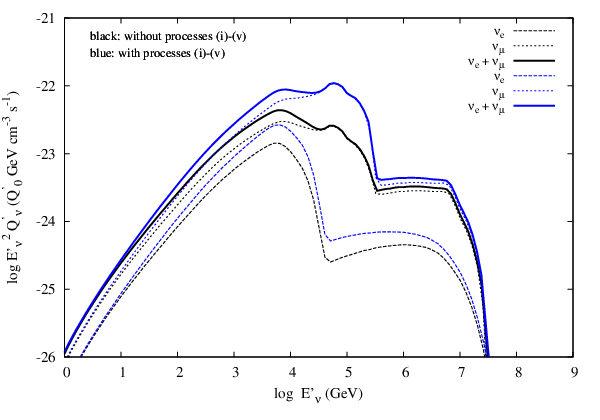
Plugging into eq. (5) the parameter values used here, we find , i.e. our study case is optically thin to photopion interactions. This suggests that interactions do not significantly affect the neutrino spectra. We verified that among all processes examined here, it is the injection of secondaries, which produce more target-photons through synchrotron radiation and/or inverse Compton scattering, that modifies at most the neutrino spectra. The effects of such additional processes on the neutrino spectra can be treated only by PDE solver codes, and requires a wider search of the parameter space.