Cooperative Beamforming for Cognitive Radio-Based Broadcasting Systems with Asynchronous InterferencesThanks: This work is supported by the Natural Science and Engineering Research Council (NSERC) of Canada, and will be presented in part at the IEEE Wireless Communications and Networking Conference (WCNC’14), Istanbul, Turkey, April 2014.

Mai H. Hassan² and Md. Jahangir Hossain⁴ Affiliation: ²Department of Electrical and Computer Engineering
The University of British Columbia, Vancouver, BC, Canada
⁴School of Engineering
The University of British Columbia, Kelowna, BC, Canada
maih@ece.ubc.ca, jahangir.hossain@ubc.ca Affiliation:

Abstract

In a cooperative cognitive radio (CR) network, cooperative beamforming can enable concurrent transmissions of both primary and secondary systems at a given channel. However, such cooperative beamforming can introduce asynchronous interferences at the primary receivers as well as at the secondary receivers and these asynchronous interferences are overlooked in beamforming design. In order to address the asynchronous interference issue for a generalized scenario with multiple primary and multiple secondary receivers, in this paper, we propose an innovative cooperative beamforming technique. In particular, the cooperative beamforming design is formulated as an optimization problem that maximizes the weighted sum achievable transmission rate of secondary destinations while it maintains the asynchronous interferences at the primary receivers below their target thresholds. In light of the intractability of the problem, we propose a two-phase suboptimal cooperative beamforming technique. First, it finds the beamforming directions corresponding to different secondary destinations. Second, it allocates the power among different beamforming directions. Due to the multiple interference constraints corresponding to multiple primary receivers, the power allocation scheme in the second phase is still complex. Therefore, we also propose a low complex power allocation algorithm. The proposed beamforming technique is extended for the cases, when cooperating CR nodes (CCRNs) have statistical or erroneous channel knowledge of the primary receivers. We also investigate the performance of joint CCRN selection and beamforming technique. The presented numerical results show that the proposed beamforming technique can significantly reduce the asynchronous interference signals at the primary receivers and increase the sum transmission rate of secondary destinations compared to the well known zero-forcing beamforming (ZFBF) technique.

I Introduction

Recently dynamic spectrum access (DSA) or opportunistic spectrum access policy has received a great deal of attention in order to improve the overall spectrum utilization. Cognitive radio (CR) [1], [2] is one of the key enabling technologies in order to facilitate DSA. Different DSA mechanisms have already been envisioned and studied in the literature [3], [4]. Among these, two approaches namely, underlay and overlay spectrum access mechanisms for spectrum sharing between primary and secondary systems have been considered widely. The underlay spectrum access mechanism [4] allows simultaneous sharing of underutilized frequency bands by a secondary/CR system along with a primary system provided that the introduced interference to the primary users does not exceed certain thresholds specified by the primary system or the regulatory authority, see for example [5] for details.

Cooperation among nodes in a wireless network can improve the overall performances [6, 7]. For example, small nodes with simple omni-directional antenna can cooperatively emulate a large highly directional antenna array which is referred to as cooperative transmit beamforming. In other words, in order to send a common message, a number of single antenna-based nodes in a wireless network organize themselves into a virtual antenna array and focus their transmission in the direction of the intended receivers. Such beamforming technique has been proposed and studied for traditional wireless communication networks e.g., wireless sensor network as this potentially offers large increases in energy efficiency, in attainable range and transmission rate, see for example [8] and the references therein. With such cooperative beamforming technique, the achievable data rate gain is quite compelling in spite of certain costs associated with it e.g., synchronising the sensor nodes and the local exchange of sensor nodes’ observations [9].

In order to reap the benefit of cooperative communications, cooperative beamforming technique has been proposed for CR systems as well [10, 11, 12]. In fact cooperative transmit beamforming can be very effective for CR systems that work based on underlay spectrum access mechanism which imposes severe constraints on the transmission power of CR systems [4]. For example, if a cognitive/secondary transmitter¹¹ 1 In the literature CR users are also referred to as secondary users and throughout this paper the words secondary and cognitive have been used interchangeably. wants to broadcast a common message to a group of secondary destinations, the transmitter may not be allowed to transmit enough power to cover all the destinations due to the interference restriction imposed by the nearby primary system. In such situation, a group of secondary nodes which are referred to as cooperating cognitive radio nodes (CCRNs) can collaboratively use transmit beamforming to broadcast the common message to the secondary destinations see for example [10]. Using an innovative orthogonal projection technique, the authors in [10] obtained the so-called zero forcing beamforming (ZFBF) weights of the CCRNs to null the interference at the primary receivers. Using the ZFBF technique, the authors in [11] proposed a cross-layer optimization of the transmission rate and scheduling scheme of the data packets at the secondary source and at the CCRNs in the CR network. In [12], power allocation for cooperative CR networks was studied, along with user selection under imperfect spectrum sensing.

Given the fact that in practice, different CCRNs are usually located in different geographical locations, their signals can arrive with different propagation delays at each primary receiver and at each secondary receiver. Therefore with such cooperative beamforming, simultaneous transmissions from the CCRNs can cause asynchronous interferences which are discussed in details in Section II-B. Although the cooperative beamforming technique can improve the overall performance of CR systems, the asynchronous interferences are overlooked in designing beamforming technique. As we will see later in this paper that the ZFBF technique introduces a significant amount of asynchronous interference power at the primary receivers.

The asynchronous interference issue for conventional cooperative multi-cell mobile networks has been studied in [13], where multiple base stations (BSs) cooperate together to simultaneously transmit information to each mobile user in the network. However in cooperative beamforming for CR systems, the design goal is different and a new beamforming technique is required. In our earlier work [14] (the conference version published in [15]) considering the asynchronous interference, we developed a cooperative beamforming technique for a CR network with one secondary destination and one primary receiver.

As a follow-up of our initial work [14], in this paper we consider a more generalized setup where a group of CCRNs uses cooperative beamforming technique to broadcast common message to multiple secondary destinations using a wireless communication channel that is used by a primary transmitter to transmit information to multiple primary receivers simultaneously. It is also considered that these primary receivers have different interference constraints in general. With multiple primary and secondary receivers, asynchronous interferences are introduced not only at the primary receivers but also at the secondary destinations except one secondary destination. Due to these asynchronous interferences, the optimal beamforming technique developed in our earlier work [14] can not be extended for a generalized system with multiple primary and multiple secondary receivers. In fact, the optimal beamforming techique is intractable due to the non-convexity and non-linearity of the problem. Even then development of suboptimal beamforming technique is complex due to multiple interference constraints corresponding to multiple primary receivers which is discussed later. In order to address the asynchronous interference issues for such a generalized scenario, in this paper, we develop innovative cooperative beamforming techniques. In particular, the contributions of this paper can be summarized as follows:

•

For a generalized scenario, the cooperative beamforming design is formulated as an optimization problem that maximizes the weighted sum achievable transmission rate of secondary destinations while it maintains the interference thresholds at the primary receivers. Due to the non-convexity and non-linearity of formulated optimization problem, we propose a two-phase suboptimal beamforming technique. First, it finds the beamforming direction corresponding to a secondary destination that maximizes the received signal power at that secondary destination while it minimizes the asynchronous interference power at other secondary destinations and at all primary receivers. Second, it allocates the power among different beamforming directions to maintain the interference constraints at the primary receivers. Due to the multiple interference constraints, the power allocation scheme in second phase can be complex as discussed later. Therefore, we also propose a low complex power allocation (LCPA) scheme. The presented numerical results show that the developed cooperative beamforming technique can increase the sum data rate of the secondary destinations up to 64% compared to the well-known ZFBF technique.
•

We extend the proposed cooperative beamforming technique to the case of having only partial channel state information (CSI) between the primary receivers and the CCRNs. This partial CSI has been modeled by two scenarios. In the first scenario, we consider having only statistical CSI of the channels. In this case, the asynchronous interferences at the primary receivers are guaranteed in a statistical sense [16], [17]. In the absence of mathematically tractable expression of the distribution of the random interference power at the primary receiver, we develop an upper bound on the probability of introducing interference at a given primary receiver beyond a given threshold. Then this developed upper bound is used to design a robust leakage beamforming (RLBF) technique. The second scenario considers of having erroneous CSI. For both scenarios, we design RLBF techniques that can protect the primary network’s functionality by satisfying the interference constraints at all primary receivers in the network, in spite of the partial knowledge of CSI.
•

We also investigate the performance of joint CCRN selection and beamforming technique. The numerical results show that CCRN selection in conjunction with beamforming can further increase the sum transmission rate of secondary destinations significantly.

The rest of the paper is organized as follows. In Section II we present the overall system description and model the asynchronous interference signals at the primary receivers as well as at the secondary destinations mathematically. While in Section III we develop the beamforming techniques with perfect CSI at the CCRNs, in Section IV, we develop robust beamforming techniques for two scenarios, i.e., imperfect channel CSI and statistical CSI. In Section V, we investigate the performance of joint CCRN selection and cooperative beamforming. Section VI presents some numerical examples. Finally, Section VII concludes the paper.

II System Model

II-A Overall Description and Operating Assumptions

For an example, the cooperative beamforming for CR-based broadcasting system is shown in Fig. 1 where a group of $L$ CCRNs uses a transmit beamforming technique to transmit common information to a group of $K$ secondary destinations. All nodes are assumed to be equipped with single antenna. As we mentioned earlier that similar type of cooperative beamforming scenario is considered for traditional wireless networks e.g., wireless sensor network due to its compelling gain in the transmission rate, see for example [8], [9]. Using the underlay spectrum access mechanism, the CR system shares a communication channel with a primary transmitter e.g., a primary BS that transmits information to $J$ primary receivers simultaneously. For notational convenience, $K$ secondary destinations are denoted by d ${}_{k},k=1,\cdots,K$ , $L$ CCRNs are denoted by c ${}_{l},~l=1,\cdots,L$ and $J$ primary receivers are denoted by p ${}_{j},~j=1,\cdots,J$ . In what follows, we provide the operating principles as well as the assumptions that we consider in our problem formulation.

Refer to caption — Fig. 1: System model for cooperative beamforming with $L$ CCRNs, $K$ secondary destinations and $J$ primary receivers.

We consider that both primary and secondary systems work in a time-slotted fashion with slot duration $T$ sec. At CCRN, c_l the information stream is mapped into modulated symbols, $x_{s}$ which has average power $P$ and the data vector consisting of these $M$ modulated symbols is denoted by $\mathbf{x}_{s}$ . We assume a block fading channel model, in which the channel fading is assumed to remain roughly the same over the time slot, but is independent of the fading in other time slots. The set of cooperative CCRNs uses $K$ different beamforming vectors to direct transmission to $K$ different secondary destinations. The received signal at secondary destination, d_k can be written as

\mathbf{y}_{k}[n]=\mathbf{h}_{k}^{\mbox{\tiny{s}}}[n]\mathbf{g}_{k}[n]\mathbf{x}_{s}[n]+\mathbf{I}_{k}[n]+\mathbf{m}_{k}[n]+\mathbf{z}_{k}[n],

(1)

where $\mathbf{x}_{s}[n]$ is common message symbols transmitted at time slot $n$ and $\mathbf{h}_{k}^{\mbox{\tiny{s}}}[n]\triangleq[h_{k1}^{\mbox{\tiny{s}}}[n],\text{\ldots},h_{kL}^{\mbox{\tiny{s}}}[n]]$ is the channel vector from $L$ transmitting CCRNs to secondary destination, d_k. The vector $\mathbf{g}_{k}[n]\triangleq[g_{k1}[n],\text{\ldots},g_{kL}[n]]^{T}$ denotes the beamforming weight vector of the set of CCRNs corresponding to transmission to secondary destination, d_k with each element $g_{kr}$ denoting the weight of the CCRN, c_r. $\mathbf{z}_{k}[n]$ is the additive white Gaussian noise (AWGN) vector at secondary destination, d_k with zero mean and two sided power spectrum density $N_{0}/2$ , and $\mathbf{m}_{k}[n]$ is the received interfering signal vector from the primary BS at secondary destination d_k. $\mathbf{I}_{k}[n]$ is the asynchronous interference signal at secondary destination, d_k resulting from the data transmissions to the other $(K-1)$ secondary destinations and can be written as follows

\mathbf{I}_{k}[n]=\sum_{i=1,i\neq k}^{K}\sum_{r=1}^{L}h_{kr}^{\mbox{\tiny{s}}}[n]g_{ir}[n]\mathbf{i}_{r}[n],

(2)

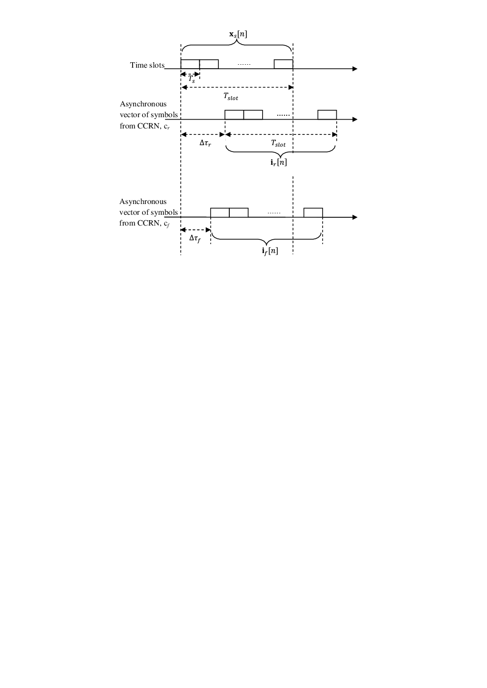
where $\mathbf{i}_{r}[n]$ is the asynchronous vector of symbols received at the secondary destination d_k from the CCRN c_r, as shown in Fig. 2.

The ZFBF technique developed in [10] did not consider the asynchronous interference issue described below. In fact, we will see later in this paper that if ZFBF technique is used in this scenario, the asynchronous interferences at the primary receivers exceed the target thresholds. So there is a need for developing an innovative beamforming technique which is the main focus of this paper.

II-B Modeling of Asynchronous Interferences

Given the fact that the CCRNs are located in different geographical locations, the received signals from different CCRNs at different primary receivers and at different secondary destinations can experience different propagation delays. Although the received signal at a particular secondary destination e.g., d₁ from different CCRNs can be synchronized by using a timing advance mechanism which is currently employed in the uplink of GSM and 3G cellular networks (see for example [13]) or other mechanism [9], the received signals at the primary receivers p_j ( $j=1,\cdots,J$ ) and at the other secondary destinations, d_k $(k=2,\cdots,K)$ cannot be synchronized simultaneously. As such, the signal transmissions from CCRNs will introduce asynchronous interference at primary receivers p_j ( $j=1,\cdots,J$ ) and at the other secondary destinations, d_k $(k=2,\cdots,K)$ . In our previous work [14], we have modeled the asynchronous interference at the primary destination with one primary receiver and one secondary destination in the system. However for the generalized scenario considered in this paper, we need to model the asynchronous interferences not only at different primary receivers but also at different secondary destinations. In what follows, we model these asynchronous interferences. For notational convenience, we will drop the time slot index $n$ .

II-B1 Asynchronous interference at primary receiver, p_j

Mathematically, the asynchronous interference power resulting from transmission to secondary destination, d_k at primary receiver, p_j, $P_{\text{asynch}}^{(j,k)}$ , can be written in the following form [14]

P_{\text{asynch}}^{(j,k)}=\sum_{r=1}^{L}\sum_{f=1}^{L}g_{kf}^{\dagger}({h_{jf}^{\mbox{\tiny{p}}}})^{\dagger}h_{jr}^{\mbox{\tiny{p}}}g_{kr}{\beta_{k}^{j}}^{(r,f)},

(3)

where $h_{jr}^{\mbox{\tiny{p}}}$ is the channel fading gain from CCRN c_r to primary receiver, p_j, ${\beta_{k}^{j}}^{(r,f)}$ is the correlation between the asynchronous symbols of CCRNs, c_r and c_f at primary receiver, p_j corresponding to the transmission to secondary destination, d_k. The value of ${\beta_{k}^{j}}^{(r,f)}$ can be calculated for given propagation delays between CCRNs, c_r and c_f to primary receiver, p_j using the same technique described in [14]. Now the total asynchronous interference power at primary receiver, p_j can be expressed as

P^{j}_{\text{asynch}}=\sum_{k=1}^{K}\sum_{r=1}^{L}\sum_{f=1}^{L}g_{kf}^{\dagger}(h_{jf}^{\mbox{\tiny{p}}})^{\dagger}h_{jr}^{\mbox{\tiny{p}}}g_{kr}{\beta_{k}^{j}}^{(r,f)}.

(4)

The asynchronous interference power at primary receiver, p_j in eq. (4) can be rewritten in a matrix form as follows

P^{j}_{\text{asynch}}=\sum_{k=1}^{K}{\mathbf{g}_{k}}^{\dagger}\mathbf{R}_{k}^{j}\mathbf{g}_{k}

(5)

where $\mathbf{R}_{k}^{j}$ is expressed as

\mathbf{R}_{k}^{j}=\left[\begin{array}[]{ccc}{\beta_{k}^{j}}^{(1,1)}(h_{j1}^{\mbox{\tiny{p}}})^{\dagger}h_{j1}^{\mbox{\tiny{p}}}&\negthickspace\cdots&{\beta_{k}^{j}}^{(1,L)}(h_{j1}^{\mbox{\tiny{p}}})^{\dagger}h_{jL}^{\mbox{\tiny{p}}}\\ {\beta_{k}^{j}}^{(2,1)}(h_{j2}^{\mbox{\tiny{p}}})^{\dagger}h_{j1}^{\mbox{\tiny{p}}}&\negthickspace\cdots&{\beta_{k}^{j}}^{(2,L)}(h_{j2}^{\mbox{\tiny{p}}})^{\dagger}h_{jL}^{\mbox{\tiny{p}}}\\ \negthickspace\vdots&\negthickspace\ddots&\negthickspace\vdots\\ {\beta_{k}^{j}}^{(L,1)}(h_{jL}^{\mbox{\tiny{p}}})^{\dagger}h_{j1}^{\mbox{\tiny{p}}}&\negthickspace\cdots&{\beta_{k}^{j}}^{(L,L)}(h_{jL}^{\mbox{\tiny{p}}})^{\dagger}h_{jL}^{\mbox{\tiny{p}}}\end{array}\right].

(6)

The received signal power at secondary destination, d_k is given by

P_{k,\text{signal}}=P{\mathbf{g}_{k}}^{\dagger}(\mathbf{h}_{k}^{\mbox{\tiny{s}}})^{\dagger}\mathbf{h}_{k}^{\mbox{\tiny{s}}}\mathbf{g}_{k}.

(7)

II-B2 Asynchronous interference at secondary destination, d_k

The asynchronous interference power at secondary destination, d_k resulting from transmission to secondary destination, d_i is given by

\mbox{AI}^{k}_{i}=\sum_{r=1}^{L}\sum_{f=1}^{L}{\beta^{k}_{i}}^{(r,f)}g_{if}^{\dagger}(h_{kf}^{\mbox{\tiny{s}}})^{\dagger}h_{kr}^{\mbox{\tiny{s}}}g_{ir},

(8)

where ${\beta_{i}^{k}}^{(r,f)}$ is the correlation between the asynchronous symbols of CCRNs, c_r and c_f at secondary destination, d_i corresponding to the transmission to secondary destination, d_k where $k\neq i$ . The value of ${\beta_{i}^{k}}^{(r,f)}$ can be calculated for given propagation delays between CCRNs, c_r and c_f to secondary destinations, d_i and d_k using the same method described in [14]. Therefore, the total asynchronous interference power at secondary destination, d_k resulting from data transmission to the other $(K-1)$ secondary destinations, AI^k can be written as

\mbox{AI}^{k}=\sum_{i=1,i\neq k}^{K}\sum_{r=1}^{L}\sum_{f=1}^{L}{\beta^{k}_{i}}^{(r,f)}g_{if}^{\dagger}(h_{kf}^{\mbox{\tiny{s}}})^{\dagger}h_{kr}^{\mbox{\tiny{s}}}g_{ir}.

(9)

Similar to eq. (7), AI^k can be written in a matrix form as follows

\mbox{AI}^{k}=\sum_{i=1,i\neq k}^{K}\mathbf{g}_{i}^{\dagger}\mathbf{T}^{k}_{i}\mathbf{g}_{i},

(10)

where $\mathbf{T}^{k}_{i}$ is written as

\mathbf{T}^{k}_{i}\triangleq\left[\begin{array}[]{ccc}{\beta^{k}_{i}}^{(1,1)}(h_{k1}^{\mbox{\tiny{s}}})^{\dagger}h_{k1}^{\mbox{\tiny{s}}}&\cdots&{\beta^{k}_{i}}^{(1,L)}(h_{k1}^{\mbox{\tiny{s}}})^{\dagger}h_{kL}^{\mbox{\tiny{s}}}\\ \vdots&\ddots&\vdots\\ {\beta^{k}_{i}}^{(L,1)}(h_{kL}^{\mbox{\tiny{s}}})^{\dagger}h_{k1}^{\mbox{\tiny{s}}}&\cdots&{\beta^{k}_{i}}^{(L,L)}(h_{kL}^{\mbox{\tiny{s}}})^{\dagger}h_{kL}^{\mbox{\tiny{s}}}\end{array}\right].

III Beamforming Design with Perfect Channel Knowledge

In this section, we develop a new beamforming technique, called cooperative leakage beamforming (LBF) technique in order to address the problem of asynchronous interferences at the primary receivers and other secondary destinations. In this development, we use the same assumption as in [10, 18, 19, 20] that the channel fading gains, i.e., instantaneous CSI between the CCRNs and the primary receivers as well as the instantaneous CSI between the CCRNs and the secondary destinations are known perfectly at the CCRNs. Different possible scenarios have been considered in the literature in order to estimate the CSI between the CCRNs and the primary receivers (see for examples, [21], [22]). In the next section, we consider the case when the CSI between the CCRNs and the primary receivers are not known perfectly.

III-A Problem Formulation

The achievable transmission rate of secondary destination d_k, $r_{k}$ can be expressed using the ideal capacity formula as follows

r_{k}=\log_{2}\Biggl(1+\frac{P\mathbf{g}_{k}^{\dagger}(\mathbf{h}_{k}^{\mbox{\tiny{s}}})^{\dagger}\mathbf{h}_{k}^{\mbox{\tiny{s}}}\mathbf{g}_{k}}{\sigma_{k}^{2}+{\displaystyle\sum_{i=1,i\neq k}^{K}\mathbf{g}_{i}^{\dagger}\mathbf{T}^{k}_{i}\mathbf{g}_{i}}}\Biggr),

(11)

where $\sigma_{k}^{2}$ is the power of the AWGN plus the interference power from the primary transmitter at secondary destination d_k. The goal is to design $K$ different beamforming vectors corresponding to $K$ secondary destinations that maximize the weighted sum rate of all secondary destinations while keeping the interference to the primary receivers below their target thresholds. We consider maximizing the weighted sum rate of all the $K$ secondary destinations since it is more generalized (see for example [23], and the references therein). The design goal can be formulated as an optimization problem as follows²² 2 We do not consider transmit power constraint for the CCRNs as we develop the beamforming technique for the interference limited scenario.

	$\displaystyle\mathbf{g}_{1}^{\text{\tiny{(opt)}}},\mathbf{g}_{2}^{\text{\tiny{(opt)}}},\cdots,\mathbf{g}_{K}^{\text{\tiny{(opt)}}}$	$\displaystyle=$	$\displaystyle\max_{\mathbf{g}_{1},\cdots,\mathbf{g}_{K}}\sum_{k=1}^{K}w^{k}\log_{2}\Biggl(1+\frac{P\mathbf{g}_{k}^{\dagger}(\mathbf{h}_{k}^{\mbox{\tiny{s}}})^{\dagger}\mathbf{h}_{k}^{\mbox{\tiny{s}}}\mathbf{g}_{k}}{\sigma_{k}^{2}+{\displaystyle\sum_{i=1,i\neq k}^{K}\mathbf{g}_{i}^{\dagger}\mathbf{T}^{k}_{i}\mathbf{g}_{i}}}\Biggr),$
	subject to:		$\displaystyle\sum_{k=1}^{K}\mathbf{g}_{k}^{\dagger}\mathbf{R}_{k}^{j}\mathbf{g}_{k}\leq\gamma^{j}_{\text{th}},\text{for }j=1,\cdots,J.$		(12)

where $w^{k}$ is the weighting factor of secondary destination d_k, and $\gamma^{j}_{\text{th}}$ is the required interference threshold for primary receiver, p_j.

III-B Development of Suboptimal Cooperative LBF Technique

The optimization problem in eq. (12) is a non-linear and non-convex optimization problem due to the presence of the interference power AI ${}^{k}=\sum_{i=1,i\neq k}^{K}\mathbf{g}_{i}^{\dagger}\mathbf{T}^{k}_{i}\mathbf{g}_{i}$ in secondary destination d_k’s transmission rate, $r_{k}$ . In light of the intractability of this optimization problem, we propose a two-phase suboptimal cooperative LBF technique as described below.

III-B1 Phase I

In this phase, we find the direction of the normalized beamforming vector, $\mathbf{\bar{g}}_{k}$ that maximizes the received signal power at secondary destination d_k while it minimizes the interference at all primary receivers and other secondary destinations. This can be written as the following optimization problem

\displaystyle\mathbf{\bar{g}}_{k}^{\text{\tiny{(LBF)}}}

\displaystyle=

\displaystyle\max_{\mathbf{\bar{g}}_{k}}\frac{\mathbf{\bar{g}}_{k}^{\dagger}(\mathbf{h}_{k}^{\mbox{\tiny{s}}})^{\dagger}\mathbf{h}_{k}^{\mbox{\tiny{s}}}\mathbf{\bar{g}}_{k}}{\mathbf{\bar{g}}_{k}^{\dagger}\bigl(\mathbf{R}_{k}+\mathbf{T}_{k}\bigr)\mathbf{\bar{g}}_{k}},\text{\;\;\;\;\;\;for }k=1,\cdots,K,

(13)

where $\mathbf{T}_{k}=\sum_{i=1,i\neq k}^{K}\mathbf{T}^{i}_{k}$ and $\mathbf{R}_{k}=\sum_{j=1}^{J}\mathbf{R}^{j}_{k}$ . The signal-to-leakage power ratio in eq. (13) is in the form of a generalized Rayleigh quotient, that is maximized when $\mathbf{\bar{g}}_{k}^{\text{\tiny{(LBF)}}}$ is the normalized eigen vector of the matrix ${\bigl(\mathbf{R}_{k}+\mathbf{T}_{k}\bigr)}^{-1}(\mathbf{h}_{k}^{\mbox{\tiny{s}}})^{\dagger}\mathbf{h}_{k}^{\mbox{\tiny{s}}}$ that corresponds to its maximum eigen value [24]. As indicated before, the optimization problem in eq. (12) is a non-linear and non-convex optimization problem which cannot be solved optimally, due to the presence of the asynchronous interference power AI^k. By minimizing such interference and for mathematical tractability, we neglect the interference power at secondary destination d_k. In Section VI, we will show that after minimizing the asynchronous interference power at the secondary destinations, the remaining asynchronous interference power has a negligible effect on transmission rate $r_{k}$ . So by neglecting the asynchronous interference power AI^k, the transmission rate $r_{k}$ can be now approximated as

r_{k}^{\mbox{\tiny{App}}}\approx\log_{2}\Bigl(1+\frac{P\mathbf{\alpha}_{k}\mathbf{\bar{g}}_{k}^{\text{\tiny{(LBF)}}{\dagger}}(\mathbf{h}_{k}^{\mbox{\tiny{s}}})^{\dagger}\mathbf{h}_{k}^{\mbox{\tiny{s}}})\mathbf{\bar{g}}_{k}^{\text{\tiny{(LBF)}}}}{\sigma_{k}^{2}}\Bigr),

(14)

where $\mathbf{\alpha}_{k}$ is the power allocated to the beamforming direction corresponding to secondary destination d_k.

III-B2 Phase II

In this phase, we propose to allocate power $\mathbf{\alpha}_{k}^{\text{\tiny{(LBF)}}}$ among different beamforming directions. As such the approximated weighted sum rate of secondary destinations is maximized while the interference thresholds at different primary receivers are met. In particular, given the normalized beamforming vector $\mathbf{\bar{g}}_{k}^{\text{\tiny{(LBF)}}}$ obtained in Phase-I, we obtain its allocated power $\mathbf{\alpha}_{k}^{\text{\tiny{(LBF)}}}$ that satisfies the interference threshold at all primary receivers simultaneously, where $\mathbf{{g}}_{k}^{\text{\tiny{(LBF)}}}=\sqrt{\alpha_{k}^{\text{\tiny{(LBF)}}}}\mathbf{\bar{g}}_{k}^{\text{\tiny{(LBF)}}}$ . So the power allocation problem for given beamforming directions can be written as

	$\displaystyle\mathbf{\alpha}_{1}^{\text{\tiny{(LBF)}}},\mathbf{\alpha}_{2}^{\text{\tiny{(LBF)}}},\cdots,\mathbf{\alpha}_{K}^{\text{\tiny{(LBF)}}}$	$\displaystyle=$	$\displaystyle\max_{\mathbf{\alpha}_{1},\cdots,\mathbf{\alpha}_{K}}\sum_{k=1}^{K}w^{k}\log_{2}\Bigl(1+\frac{P\alpha_{k}\mathbf{\bar{g}}_{k}^{\text{\tiny{(LBF)}}{\dagger}}(\mathbf{h}_{k}^{\mbox{\tiny{s}}})^{\dagger}\mathbf{h}_{k}^{\mbox{\tiny{s}}}\mathbf{\bar{g}}_{k}^{\text{\tiny{(LBF)}}}}{\sigma_{k}^{2}}\Bigr),$
	subject to:		$\displaystyle\sum_{k=1}^{K}\alpha_{k}\mathbf{\bar{g}}_{k}^{\text{\tiny{(LBF)}}{\dagger}}\mathbf{R}_{k}^{j}\mathbf{\bar{g}}_{k}^{\text{\tiny{(LBF)}}}\leq\gamma^{j}_{\text{th}},~~\text{for }j=1,\cdots,J.$		(15)

The Lagrange function of the above optimization problem can be written as

\mathcal{L}=\sum_{k=1}^{K}w^{k}\log_{2}\Bigl(1+\frac{P\alpha_{k}\mathbf{\bar{g}}_{k}^{\text{\tiny{(LBF)}}{\dagger}}(\mathbf{h}_{k}^{\mbox{\tiny{s}}})^{\dagger}\mathbf{h}_{k}^{\mbox{\tiny{s}}}\mathbf{\bar{g}}_{k}^{\text{\tiny{(LBF)}}}}{\sigma_{k}^{2}}\Bigr)-\sum_{j=1}^{J}\biggl(\lambda^{j}\bigl(\sum_{k=1}^{K}\alpha_{k}\mathbf{\bar{g}}_{k}^{\text{\tiny{(LBF)}}{\dagger}}\mathbf{R}_{k}^{j}\mathbf{\bar{g}}_{k}^{\text{\tiny{(LBF)}}}-\gamma^{j}_{\text{th}}\bigr)\biggr),

(16)

where $\{\lambda^{1},\cdots,\lambda^{J}\}$ are the Lagrange multipliers. Using KKT conditions, we can write

w^{k}{\Bigl(\alpha_{k}+\frac{\sigma_{k}^{2}}{P\mathbf{\bar{g}}_{k}^{\text{\tiny{(LBF)}}{\dagger}}(\mathbf{h}_{k}^{\mbox{\tiny{s}}})^{\dagger}\mathbf{h}_{k}^{\mbox{\tiny{s}}}\mathbf{\bar{g}}_{k}^{\text{\tiny{(LBF)}}}}\Bigr)}^{-1}-\sum_{j=1}^{J}\biggl(\lambda^{j}\mathbf{\bar{g}}_{k}^{\text{\tiny{(LBF)}}{\dagger}}\mathbf{R}_{k}^{j}\mathbf{\bar{g}}_{k}^{\text{\tiny{(LBF)}}}\biggr)=0\;\;\;\;\;\;\text{for }k=1,\cdots,K,

(17)

\lambda^{j}\bigl(\sum_{k=1}^{K}\alpha_{k}\mathbf{\bar{g}}_{k}^{\text{\tiny{(LBF)}}{\dagger}}\mathbf{R}_{k}^{j}\mathbf{\bar{g}}_{k}^{\text{\tiny{(LBF)}}}-\gamma^{j}_{\text{th}}\bigr)=0,\;\;\;\;\;\;\;\;\;\;\;\;\text{for }j=1,\cdots,J,

(18)

\sum_{k=1}^{K}\alpha_{k}\mathbf{\bar{g}}_{k}^{\text{\tiny{(LBF)}}{\dagger}}\mathbf{R}_{k}^{j}\mathbf{\bar{g}}_{k}^{\text{\tiny{(LBF)}}}-\gamma^{j}_{\text{th}}\leq 0,\;\;\;\;\;\;\;\;\;\;\;\;\text{for }j=1,\cdots,J,

(19)

\lambda^{1},\cdots,\lambda^{J}\geq 0,

(20)

According to eq. (17), the power allocation for beamforming direction corresponding to secondary destination d_k is given by

\alpha_{k}^{\text{\tiny{(LBF)}}}=\max\Biggl(0,\frac{w^{k}}{\sum_{j=1}^{J}\biggl(\lambda^{j}\mathbf{\bar{g}}_{k}^{\text{\tiny{(LBF)}}{\dagger}}\mathbf{R}_{k}^{j}\mathbf{\bar{g}}_{k}^{\text{\tiny{(LBF)}}}\biggr)}-\frac{\sigma_{k}^{2}}{P\mathbf{\bar{g}}_{k}^{\text{\tiny{(LBF)}}{\dagger}}(\mathbf{h}_{k}^{\mbox{\tiny{s}}})^{\dagger}\mathbf{h}_{k}^{\mbox{\tiny{s}}}\mathbf{\bar{g}}_{k}^{\text{\tiny{(LBF)}}}}\Biggr),

(21)

for $k=1,\cdots,K$ . The power allocation in eq. (21) is the cap-limited water-filling solution. In eq. (21), the power allocation values $\alpha_{k}^{\text{\tiny{(LBF)}}}$ are expressed in terms of Lagrange multipliers $\lambda_{j}$ $(j=1,\cdots,J$ ) which need to be evaluated.

In order to obtain the Lagrange multipliers and consequently $\alpha_{k}^{\text{\tiny{(LBF)}}}$ , a recursive technique is used as described below. First, we assume that only one Lagrange multiplier is greater then zero, i.e., $\lambda^{j}>0$ , while $\lambda^{i}=0$ , for all $i$ except $i\neq j$ . This implies that the optimum power allocation values $\alpha_{k}^{\text{\tiny{(LBF)}}}$ , $(k=1,\cdots,K)$ , satisfy the interference threshold with equality only at primary receiver p_j. For this case, we can write

\sum_{k=1}^{K}\alpha_{k}^{\text{\tiny{(LBF)}}}\mathbf{\bar{g}}_{k}^{\text{\tiny{(LBF)}}{\dagger}}\mathbf{R}_{k}^{j}\mathbf{\bar{g}}_{k}^{\text{\tiny{(LBF)}}}-\gamma^{j}_{\text{th}}=0.

(22)

Now the value of $\lambda^{j}$ and the power allocation values $\alpha_{k}^{\text{\tiny{(LBF)}}}$ , for all $k$ are found by solving set of equations in (21) and (22) simultaneously. If these values of $\alpha_{k}^{\text{\tiny{(LBF)}}}$ satisfy the remaining $(J-1)$ interference constraints given by the set of equations in (19), then $\alpha_{k}^{\text{\tiny{(LBF)}}}$ for all $k$ represent the optimum solution of (15). Otherwise, we set $\lambda^{k}>0$ ( $k\neq j)$ while $\lambda^{i}=0$ , for all $i$ except $i\neq k$ , and so on until we find the power allocation values that satisfy all constraints simultaneously.

If no power allocation values that satisfy all constraints simultaneously is found, considering one constraint as equality constraint we consider the case when two constraints are met with equality. In other words, we set simultaneously $\lambda^{j}>0$ and $\lambda^{l}>0$ while $\lambda^{i}=0$ , for all $i$ except $i\neq j,l$ . Then, the following two slackness conditions in eq. (18) are satisfied as follows

	$\displaystyle\sum_{k=1}^{K}\alpha_{k}^{\text{\tiny{(LBF)}}}\mathbf{\bar{g}}_{k}^{\text{\tiny{(LBF)}}{\dagger}}\mathbf{R}_{k}^{j}\mathbf{\bar{g}}_{k}^{\text{\tiny{(LBF)}}}-\gamma^{j}_{\text{th}}=0,$		(23)
	$\displaystyle\sum_{k=1}^{K}\alpha_{k}^{\text{\tiny{(LBF)}}}\mathbf{\bar{g}}_{k}^{\text{\tiny{(LBF)}}{\dagger}}\mathbf{R}_{k}^{l}\mathbf{\bar{g}}_{k}^{\text{\tiny{(LBF)}}}-\gamma^{l}_{\text{th}}=0.$		(24)

The values of $\lambda^{j}$ , $\lambda^{l}$ and the power allocation values $\alpha_{k}^{\text{\tiny{(LBF)}}}$ for all $k$ are found by solving the set of equations in (21), (23), and (24) simultaneously. If these values of $\alpha_{k}^{\text{\tiny{(LBF)}}}$ satisfy the remaining $(J-2)$ interference constraints given by the set of equations in (19), then $\alpha_{k}^{\text{\tiny{(LBF)}}}$ for all $k$ are the optimum power allocation values. Otherwise, we set another set of two constraints as equality constraint, i.e., $\lambda^{m}>0$ and $\lambda^{n}>0$ ( $m,n\neq j,l)$ while $\lambda^{i}=0$ , for all $i$ except $i\neq m,n$ , and so on until we find the values of $\alpha_{k}^{\text{\tiny{(LBF)}}}$ that satisfy all constraints simultaneously. The worst case scenario in terms of complexity occurs when the $J$ constraints hold with equality simultaneously.

This procedure is summarized below:

for

i=1\to J

- Form

\binom{J}{i}

different sets, such that each set

\mathcal{S}_{k}^{i}\text{ for }k=1,\cdots,\binom{J}{i}

is composed of

i

different

\lambda

’s.

for

j=1\to\binom{J}{i}

-Assume that

\lambda^{m}=0\text{ for }\lambda^{m}\not\in\mathcal{S}_{j}^{i}

, and that

\lambda^{n}>0

for

\lambda^{n}\in\mathcal{S}_{j}^{i}

, which implies that

the interference constraints at

i

primary receivers are satisfied with equality

simultaneously.

-Substitute these

\lambda

’s in eq. (21), and in the slackness conditions given in eqs. (18) to

get the optimum power allocation,

\alpha_{k}^{\text{\tiny{(LBF)}}}

for all

k

-Check whether the total interference introduced due to the transmissions to

K

seco-

ndary destinations satisfies the other

(J-i)

interference constraints given in eqs. (19),

- if yes, exit. Otherwise, continue.

end for

III-C Low Complexity Power Allocation Scheme

The complexity of the power allocation scheme proposed in Section III-B2 can, in the worst case scenario, be in the order of $\frac{J(J+1)}{2}$ . The optimum power allocation (OPA) scheme, proposed in Section III-B2, jointly finds all the $K$ allocated power values which can, in the worst case, require solving the $J$ interference constraints simultaneously. Therefore, we also propose a low complexity power allocation (LCPA) scheme as described below.

Rather than finding the power allocation value $\mathbf{\alpha}_{k}$ by keeping all the $J$ interference constraints simultaneously in eq. (15), we propose to find the power allocation value for only one interference constraint e.g., $j$ th interference constraint at a time. For notational convenience let us denote, the corresponding power value by $\mathbf{\alpha}_{k}^{j,\text{\tiny{LCPA}}}$ $(k={1,\cdots,K})$ which can be written as follows

\alpha_{k}^{j,\text{\tiny{LCPA}}}=\max\Biggl(0,\frac{w^{k}}{\lambda^{j}\mathbf{\bar{g}}_{k}^{\text{\tiny{(LBF)}}{\dagger}}\mathbf{R}_{k}^{j}\mathbf{\bar{g}}_{k}^{\text{\tiny{(LBF)}}}}-\frac{\sigma_{k}^{2}}{P\mathbf{\bar{g}}_{k}^{\text{\tiny{(LBF)}}{\dagger}}(\mathbf{h}_{k}^{\mbox{\tiny{s}}})^{\dagger}\mathbf{h}_{k}^{\mbox{\tiny{s}}}\mathbf{\bar{g}}_{k}^{\text{\tiny{(LBF)}}}}\Biggr).

(25)

The value of $\lambda^{j}$ is found from the following complementary slackness condition

\lambda^{j}\bigl(\sum_{k=1}^{K}\alpha_{k}^{j,\text{\tiny{LCPA}}}\mathbf{\bar{g}}_{k}^{\text{\tiny{(LBF)}}{\dagger}}\mathbf{R}_{k}^{j}\mathbf{\bar{g}}_{k}^{\text{\tiny{(LBF)}}}-\gamma^{j}_{\text{th}}\bigr)=0,\;\;\;\;\;\;\;\;\;\;\;\;\text{for }j=1,\cdots,J.

(26)

So, now for a given beamforming direction correspond a particular secondary destination d_k, we have $J$ power values $\alpha_{k}^{j,\text{\tiny{LCPA}}}$ $(j=1,\cdots,J)$ corresponding to $J$ interference constraints. Out of these $J$ power values, the minimum power value is selected as the final power allocation value for $k$ th beamforming direction, i.e.,

\mathbf{\alpha}_{k}^{\text{\tiny{LCPA}}}=\min\bigl(\mathbf{\alpha}_{k}^{1,\text{\tiny{LCPA}}},\mathbf{\alpha}_{k}^{2,\text{\tiny{LCPA}}},\cdots,\mathbf{\alpha}_{k}^{J,\text{\tiny{LCPA}}}\bigr).

(27)

The complexity of this proposed LCPA scheme is in the order of $J$ , compared to that of the OPA scheme which is in the order of $\frac{J(J+1)}{2}$ in the worst case. This lower complexity comes at the expense of sum transmission rate of secondary destinations.

IV Beamforming with Partial Channel Knowledge

In many scenarios, the instantaneous CSI of the channels between the CCRNs and the primary receivers may not be available at the CCRNs. During the design process of the cooperative transmit beamforming, we need to account for the effects of partial channel knowledge at the CCRNs to ensure a robust protection to the primary receivers. In this section, we consider two scenarios of having partial channel knowledge. The first scenario is having the erroneous CSI of the channels between the primary users and the CCRNs due to the imperfect channel estimation. The second scenario is having only the statistical CSI of the channels between the primary users and the CCRNs rather than the instantaneous CSI. For these scenarios our goal is to design RLBF techniques.

IV-A Beamforming with Erroneous Channel Estimate

When the CCRNs have erroneous estimation of the channels between the primary receivers and the CCRNs, in order to design the RLBF technique for such scenario, we adopt the following channel estimation uncertainty model. If the channel estimation of $\mathbf{h}_{j}^{\mbox{\tiny{P}}}$ is erroneous, the estimation error can be modeled as

\mathbf{h}_{j}^{\mbox{\tiny{p}}}=\hat{\mathbf{h}}_{j}^{\mbox{\tiny{p}}}+\mathbf{e}_{j},

(28)

where $\mathbf{h}_{j}^{\mbox{\tiny{p}}}$ is the actual instantaneous channel vector between the CCRNs and primary receiver p_j, $\hat{\mathbf{h}}_{j}^{\mbox{\tiny{p}}}$ is the estimated channel vector between the CCRNs and primary receiver, p_j and $\mathbf{e}_{j}$ is the corresponding estimation error vector. Based on the accuracy of the estimation technique used, the channel estimation uncertainty can be modeled by the so-called bounded uncertainty model. The bounded uncertainty model is a well-accepted model that has been used in [25, 26, 22, 27]. It considers that the uncertainty in the channel estimation is described by a bounded region whose shape depends on the channel estimation technique used. However, a spherical uncertainty region gives the worst case estimation error model [26]. In this case, the estimation error vector is bounded by ${\left\|{\mathbf{e}_{j}}\right\|}^{2}\leq\epsilon$ .

Using the error model in eq. (28), the covariance matrix corresponding to $\mathbf{h}_{j}^{\mbox{\tiny{p}}}$ , $\mathbf{R}^{j}_{k}$ can be written as [14]

\mathbf{R}^{j}_{k}=\hat{\mathbf{R}}^{j}_{k}+\Delta^{j}_{R},

(29)

where $\hat{\mathbf{R}}^{j}_{k}$ is the estimated covariance matrix corresponding to the estimated channel fading gains between the CCRNs and primary receiver p_j and can be calculated using the estimated CSI $\hat{\mathbf{h}}_{j}$ as well as ${\beta}_{k}^{j(r,f)}$ (see eq. (6)). $\Delta^{j}_{R}$ is the covariance error matrix

\Delta_{R}^{j}\negthickspace=\negthickspace\left[\begin{array}[]{ccc}{\beta_{k}^{j}}^{(1,1)}(e_{j1})^{\dagger}e_{j1}&\negthickspace\cdots&{\beta_{k}^{j}}^{(1,L)}(e_{j1})^{\dagger}e_{jL}\\ \negthickspace\vdots&\negthickspace\ddots&\negthickspace\vdots\\ {\beta_{k}^{j}}^{(L,1)}(e_{jL})^{\dagger}e_{j1}&\negthickspace\cdots&{\beta_{k}^{j}}^{(L,L)}(e_{jL})^{\dagger}e_{jL}\end{array}\right],

(30)

and is bounded by $\left\|\Delta_{R}^{j}\right\|\leq\Psi^{j}_{R}$ , where $\Psi^{j}_{R}$ is the bound of the uncertainty region of $\hat{\mathbf{R}}^{j}_{k}$ . Since $\mathbf{R}^{j}_{k}$ is a covariance matrix, it can be factorized using Cholesky decomposition [28]. Therefore, we can write $\mathbf{R}^{j}_{k}=\mathbf{C}^{j}_{k}(\mathbf{C}^{j}_{k})^{\dagger}$ , where $\mathbf{C}^{j}_{k}$ is a lower triangular matrix. Similarly, we can write $\hat{\mathbf{R}}^{j}_{k}=\hat{\mathbf{C}}^{j}_{k}(\hat{\mathbf{C}}^{j}_{k})^{\dagger}$ . Then, the relation between $\mathbf{C}^{j}_{k}$ and $\hat{\mathbf{C}}^{j}_{k}$ can be written as

\mathbf{C}^{j}_{k}=\hat{\mathbf{C}}^{j}_{k}+\Delta^{j}_{C},\;\;\;\;\;\;\;\;\;\;\;\;\left\|\Delta^{j}_{C}\right\|\leq\Psi^{j}_{C},

(31)

where $\Psi^{j}_{C}$ is the bound of the uncertainty region of $\hat{\mathbf{C}}^{j}_{k}$ .

The total asynchronous interference at primary receiver p_j should satisfy the following condition

\sum_{k=1}^{K}\mathbf{g}_{k}^{\dagger}\mathbf{R}^{j}_{k}\mathbf{g}_{k}\leq\gamma^{j}_{\text{th}},\text{ for }j=1,\cdots,J.

(32)

Using eq. (31) in eq. (32), we can reformulate the total asynchronous interference constraint for primary receiver p_j as follows

\sum_{k=1}^{K}\left\|\mathbf{g}_{k}^{\dagger}{\mathbf{C}^{j}_{k}}\right\|^{2}\leq\gamma^{j}_{\text{th}},\text{ for }j=1,\cdots,J.

(33)

However, in order to ensure a robust design of the beamforming vector using $\mathbf{C}^{j}_{k}$ , the above constraint must be satisfied for the worst case estimate of $\mathbf{C}^{j}_{k}$ , i.e.,

\max_{\left\|\Delta^{j}_{C}\right\|}\sum_{k=1}^{K}\left\|\mathbf{g}_{k}^{\dagger}{\mathbf{C}}^{j}_{k}\right\|\leq\sqrt{\gamma^{j}_{\text{th}}}.

(34)

Using the triangle inequality and applying Cauchy-Schwartz inequality [14], we can write

\left\|\mathbf{g}_{k}^{\dagger}\mathbf{C}^{j}_{k}\right\|\leq\left\|\mathbf{g}_{k}^{\dagger}\hat{\mathbf{C}}^{j}_{k}\right\|+\left\|\mathbf{g}_{k}\right\|\left\|\Delta_{C}^{j}\right\|.

(35)

Using the maximum value of $\left\|\mathbf{g}_{k}^{\dagger}\hat{\mathbf{C}}^{j}_{k}\right\|$ given in eq. (35) and substituting it in eq. (34), the design constraint now becomes

\sum_{k=1}^{K}\left\|\mathbf{g}_{k}^{\dagger}\hat{\mathbf{C}}^{j}_{k}\right\|^{2}\leq\biggl(\sqrt{\gamma^{j}_{\text{th}}}-\sum_{k=1}^{K}\left\|\mathbf{g}_{k}\right\|\Psi^{j}_{C}\biggr)^{2}.

(36)

By using the relation between $\hat{\mathbf{R}}^{j}_{k}$ and $\hat{\mathbf{C}}^{j}_{k}$ , the design constraint in eq. (36) can finally be expressed as

\sum_{k=1}^{K}\mathbf{g}_{k}^{\dagger}\hat{\mathbf{R}}^{j}_{k}\mathbf{g}_{k}\leq\biggl(\sqrt{\gamma^{j}_{\text{th}}}-\sum_{k=1}^{K}\left\|\mathbf{g}_{k}\right\|\Psi^{j}_{C}\biggr)^{2}.

(37)

Therefore, our primal optimization problem for this RLBF technique can be written as

	$\displaystyle\hat{\mathbf{g}}_{1},\hat{\mathbf{g}}_{2},\cdots,\hat{\mathbf{g}}_{K}$	$\displaystyle=$	$\displaystyle\max_{{\mathbf{g}}_{1},\cdots,{\mathbf{g}}_{K}}\sum_{k=1}^{K}w^{k}r_{k},$
	subject to:		$\displaystyle\sum_{k=1}^{K}\mathbf{g}_{k}^{\dagger}\hat{\mathbf{R}}^{j}_{k}\mathbf{g}_{k}\leq I^{j}_{\text{th}},\text{ for }j=1,\cdots,J.$		(38)

where $I^{j}_{\text{th}}=\biggl(\sqrt{\gamma^{j}_{\text{th}}}-\sum_{k=1}^{K}\left\|\mathbf{g}_{k}\right\|\Psi^{j}_{C}\biggr)^{2}$ . The optimization problem in eq. (38) is a non-linear and non-convex problem which cannot be solved optimally. However, using a two-step procedure similar to the one described in Section III-B, a suboptimal solution for the cooperative RLBF can be obtained for the scenario when CCRNs have imperfect CSI of the primary receivers.

IV-B Beamforming with Channel Statistics

When the CCRNs have the statistical CSI³³ 3 Statistical CSI refers to distribution of CSI which is assumed to be Rayleigh and corresponding parameter. of the channels between the primary receivers and the CCRNs, the interference thresholds at the primary receivers can be guaranteed statistically. In absence of instantaneous CSI of the channel between primary receiver and a CR transmitter, such statistical interference constraint to primary receivers has been used in [16], [17]. According to this statistical asynchronous interference constraint, interference thresholds are met probabilistically as follows

\mbox{Pr}\left(P_{\text{asynch}}^{j}\geq\gamma^{j}_{\text{th}}\right)\leq\epsilon^{j},

(39)

where Pr denotes probability and $\epsilon^{j}$ is the maximum allowable probability of violating the interference threshold $\gamma^{j}_{\text{th}}$ at primary receiver p_j. Since the distribution of the random interference power $P_{\text{asynch}}^{j}$ is not available in a closed-form, the probability in the left side of eq. (39) can not be written in a closed-form in terms of average channel gains between the CCRNs and the primary receivers. In what follows we develop an upper bound on this probability value, i.e., $\mbox{Pr}\left(P_{\text{asynch}}^{j}\geq\gamma^{j}_{\text{th}}\right)$ , using the well-known Markov’s inequality, in terms of average channel fading power gains between primary receiver p_j and CCRNs.

According to the Markov’s inequality the probability that a nonnegative random variable $X$ is greater than or equal to some positive constant $a$ is upper bounded by the ratio of expected value of $X$ and $a$ i.e., Pr $(X\geq a)\leq\frac{\mbox{E}(X)}{a}$ [29]. Since the asynchronous interference power $P_{\text{asynch}}^{j}$ is a non-negative function of the random variables $h_{jr}^{\mbox{\tiny{P}}},\;r=1,\cdots,L$ , according to Markov’s inequality, the probability $\mbox{Pr}\left(P_{\text{asynch}}^{j}\geq\gamma^{j}_{\text{th}}\right)$ is upper bounded as follows

\mbox{Pr}\left(P_{\text{asynch}}^{j}\geq\gamma^{j}_{\text{th}}\right)\leq\frac{\mbox{E}\left(P_{\text{asynch}}^{j}\right)}{\gamma^{j}_{\text{th}}}

(40)

which leads to a limit on the average asynchronous interference power on primary receiver p_j (c.f. eq. (39))

\mbox{E}\left(P_{\text{asynch}}^{j}\right)\leq\epsilon^{j}\gamma^{j}_{\text{th}}.

(41)

Since the total asynchronous interference power at primary receiver p_j, $P_{\text{asynch}}^{j}$ , is the summation of the interference powers corresponding to the transmissions of different secondary destinations, the average value of the total asynchronous interference power at primary receiver p_j can be written as

\mbox{E}\left(P_{\text{asynch}}^{j}\right)=\sum_{k=1}^{K}\mbox{E}\left(P_{\text{asynch}}^{(j,k)}\right).

(42)

The interference power at p_j resulting from transmission to secondary destination d_k, $P_{\text{asynch}}^{(j,k)}$ can be written in expanded form as follows (c.f. eq. (3))

P_{\text{asynch}}^{(j,k)}=\sum_{r=1}^{L}\sum_{\begin{array}[]{c}f=1,f\neq r\end{array}}^{L}g_{kf}^{\dagger}(h_{jf}^{\mbox{\tiny{p}}})^{\dagger}h_{jr}^{\mbox{\tiny{p}}}g_{kr}{\beta_{k}^{j}}^{(r,f)}+\sum_{r=1}^{L}g_{kr}^{\dagger}\left|h^{\mbox{\tiny{p}}}_{jr}\right|^{2}g_{kr}{\beta_{k}^{j}}^{(r,r)}.

(43)

Since the channel fading coefficients between different CCRNs and primary receiver p_j are independent and have zero mean, the average value of the first term in eq. (43) is equal to zero. For the second term in eq. (43), it can be easily shown that for a Rayleigh fading channel, the the fading power gain, $\left|h^{\mbox{\tiny{p}}}_{jr}\right|^{2}$ has an exponential distribution with a mean value of $\Omega^{j}_{r}$ , where $\Omega^{j}_{r}$ . The term $\sum_{r=1}^{L}g_{kr}^{\dagger}\left|h^{\mbox{\tiny{p}}}_{jr}\right|^{2}g_{kr}{\beta^{j}}^{(r,r)}$ is a summation of $L$ independent and identically distributed (i.i.d.) exponential random variables, which is a hypo-exponential random variable, with a mean value of $\sum_{r=1}^{L}g_{kr}^{\dagger}\Omega^{j}_{r}g_{kr}{\beta^{j}}^{(r,r)}$ . Therefore the average value of $P_{\text{asynch}}^{(j,k)}$ is given by

\mbox{E}\left(P_{\text{asynch}}^{(j,k)}\right)=\sum_{r=1}^{L}g_{kr}^{\dagger}\Omega^{j}_{r}g_{kr}{\beta_{k}^{j}}^{(r,r)}.

(44)

This average interference power at primary receiver p_j can be rewritten in a matrix form as follows

\mbox{E}\left(P_{\text{asynch}}^{(j,k)}\right)=\mathbf{g}_{k}^{\dagger}\bar{\mathbf{R}}_{k}^{j}\mathbf{g}_{k}

(45)

where

\bar{\mathbf{R}}_{k}^{j}=\left[\begin{array}[]{ccc}{\beta_{k}^{j}}^{(1,1)}\Omega^{j}_{1}&\cdots&0\\ \vdots&\ddots&\vdots\\ 0&\cdots&{\beta_{k}^{j}}^{(L,L)}\Omega^{j}_{L}\end{array}\right].

(46)

Using eq. (45), eq. (41) can be written as

\sum_{k=1}^{K}\mathbf{g}_{k}^{\dagger}\bar{\mathbf{R}}_{k}^{j}\mathbf{g}_{k}\leq\epsilon^{j}\gamma^{j}_{\text{th}}.

(47)

Now the cooperative RLBF vector that maximizes the weighted sum rate of secondary destinations while satisfying the new interference constraint in eq. (47) can be formulated as an optimization problem as follows

	$\displaystyle\hat{\mathbf{g}}_{1},\hat{\mathbf{g}}_{2},\cdots,\hat{\mathbf{g}}_{K}$	$\displaystyle=$	$\displaystyle\max_{{\mathbf{g}}_{1},\cdots,{\mathbf{g}}_{K}}\sum_{k=1}^{K}w^{k}r_{k},$
	subject to:		$\displaystyle\sum_{k=1}^{K}\mathbf{g}_{k}^{\dagger}\bar{\mathbf{R}}_{k}^{j}\mathbf{g}_{k}\leq\epsilon^{j}\gamma^{j}_{\text{th}},\text{ for }j=1,\cdots,J.$		(48)

The above optimization problem is again a non-linear and non-convex optimization problem, which cannot be solved optimally. However, using the two steps procedure described in Section III-B, a suboptimal solution for the cooperative RLBF for the statistical CSI scenario can be obtained by substituting for $\gamma^{j}_{\text{th}}$ by $\epsilon^{j}\gamma^{j}_{\text{th}}$ in eq (12).

V Joint CCRN Selection and Cooperative Beamforming

Since different CCRNs are located in different geographical locations, their contributions vary significantly towards the interfering signals at the primary receivers, as well as the received signals at the secondary destinations. Intuitively, a CCRN selection strategy can further improve the performance of the cooperative beamforming algorithm. The joint design of cooperative beamforming and relay selection has been studied before for conventional cooperative networks, see for example [30] and the references therein. In our previous work in [14], we studied relay selection strategies for CR systems with a single primary receiver and a single secondary destination. In this section, for completeness of the considered system with multiple primary and multiple secondary receivers, we extend the joint design of cooperative beamforming and CCRN selection.

To formulate the CCRN selection problem mathematically, we define a CCRN selection vector $\mathbf{\mathbf{S}}$ of size $K\times 1$ , where $K$ is the number of CCRNs in the network. The elements of $\mathbf{S}$ , $s_{j}$ can take value of either $1$ or $0$ , to indicate whether the CCRN c_j has been selected for transmission or not respectively. For notational convenience, we define $\mathbf{W}$ as a diagonal matrix having its diagonal elements equal to those of vector $\mathbf{S}$ , as follows

\mathbf{W}=\text{Diag}(\mathbf{S}).

(49)

The received signal power at secondary destination d_k, $P_{k,\text{sig}}$ is given by [14]

P_{k,\text{signal}}=P{\mathbf{g}_{k}}^{\dagger}\mathbf{W}^{\dagger}(\mathbf{h}_{k}^{\mbox{\tiny{s}}})^{\dagger}\mathbf{h}_{k}^{\mbox{\tiny{s}}}\mathbf{W}\mathbf{g}_{k}.

(50)

The problem of joint CCRN selection and cooperative beamforming is considered as a mixed-integer non linear problem (MINLP), since the elements of $\mathbf{W}$ can only take a value of $0$ or $1$ . Such MINLP can be solved by decoupling it into a non-linear problem (NLP) and a mixed-integer linear problem (MILP), as in [31, 32].

Using the value of the received signal power in eq. (50) for a given relay selection matrix $\mathbf{W}$ , the beamforming vector $\mathbf{g}_{k}^{\text{\tiny{(S)}}}{\scriptstyle{(\mathbf{W})}}$ can be found from the following NLP problem:

	$\displaystyle\mathbf{g}_{1}^{\text{\tiny{(S)}}}{\scriptstyle{(\mathbf{W})}},\mathbf{g}_{2}^{\text{\tiny{(S)}}}{\scriptstyle{(\mathbf{W})}},\cdots,\mathbf{g}_{K}^{\text{\tiny{(S)}}}{\scriptstyle{(\mathbf{W})}}$	$\displaystyle=$	$\displaystyle\max_{\mathbf{g}_{1},\cdots,\mathbf{g}_{K}}\sum_{k=1}^{K}w^{k}\log_{2}\Biggl(1+\frac{P\mathbf{g}_{k}^{\dagger}\mathbf{W}^{\dagger}(\mathbf{h}_{k}^{\mbox{\tiny{s}}})^{\dagger}\mathbf{h}_{k}^{\mbox{\tiny{s}}}\mathbf{W}\mathbf{g}_{k}}{\sigma_{k}^{2}+{\displaystyle\sum_{i=1,i\neq k}^{K}\mathbf{g}_{i}^{\dagger}\mathbf{W}^{\dagger}\mathbf{T}^{k}_{i}\mathbf{W}\mathbf{g}_{i}}}\Biggr),$
	subject to:		$\displaystyle\sum_{k=1}^{K}\mathbf{g}_{k}^{\dagger}\mathbf{W}\mathbf{R}_{k}^{j}\mathbf{W}\mathbf{g}_{k}\leq\gamma^{j}_{\text{th}},~~~\text{for }j=1,\cdots,J.$		(51)

For a given CCRN selection matrix $\mathbf{W}$ , the optimization problem in eq. (51) is non-convex and non-linear similar to the one in eq. (12). Therefore, for a given CCRN selection matrix $\mathbf{W}$ , we can use the same two-phase suboptimal approach described in Section III-B to find the suboptimal ${\mathbf{g}_{k}}^{\text{\tiny{(S,sub)}}}{\scriptstyle{(\mathbf{W})}}$ for all $k$ . Then, the optimal CCRN selection matrix $\mathbf{W^{\ast}}$ and corresponding ${\mathbf{g}_{k}}^{\text{\tiny{(S,sub)}}}(\scriptstyle{\mathbf{W^{\ast}}})$ are obtained via exhaustive search over all possible selections of $\mathbf{W}$ .

The CCRN selection scheme can be further extended to the case where only partial knowledge of the channels between the primary receivers and the CCRNs is available at the CCRNs. Using similar procedures as those described in Section IV, we can jointly design the CCRN selection and the cooperative beamforming for the case of erroneous channel estimate, and having only the statistical CSI available at the CCRNs. Due to space limitation, we do not include them.

VI Numerical results

In this section, we present some selected numerical results in order to compare the performances of various beamforming techniques in the presence of asynchronous interference. For all the numerical examples presented in this section, we consider the network topology shown in Fig. 3. For the sake of simplicity, it is assumed to have $J=2$ primary receivers, $K=3$ secondary destinations and $L=4$ CCRNs. The distances between the nodes in Fig. 3 are picked up arbitrarily. Distances between other nodes and corresponding propagation delays can be obtained easily using the given distances. We assume that all the channel fading gains are identically and independently Rayleigh distributed. We consider a slot duration $T_{\text{slot}}=0.4$ msec, and a log-distance path loss model with a path loss exponent value of $4$ . The normalized average interference power from the primary transmitter to the secondary destinations, d₁, d₂ and d₃ are assumed to be $-10,-20$ , and $-15$ dB, respectively. For simplicity, we consider weighting factors $w_{1}$ , $w_{2}$ and $w_{3}$ are equal to one.

In Fig. 4, we plot the normalized symbol power versus the total asynchronous interference signal power introduced at the primary receivers using our proposed cooperative LBF technique. We assume that interference thresholds at primary receiver p₁ and p₂ are respectively, $\gamma^{1}_{\text{th}}=0.1\times 10^{-15}$ and $\gamma^{2}_{\text{th}}=0.25\times 10^{-15}$ which are in the order of the noise power. In this figure we also plot the asynchronous interference signal powers introduced at the primary receivers when ZFBF technique [10] is used. This figure clearly shows that our proposed LBF technique can maintain the asynchronous interference thresholds at the primary receivers simultaneously. On the contrary, the interference caused by the ZFBF technique exceeds the interference target thresholds at the primary receivers. This is expected as ZFBF does not take asynchronous interferences into account in its design.

In Fig. 5, we plot the achievable average sum rate of secondary destinations with the proposed cooperative LBF with OPA scheme, the LBF with LCPA scheme, and the ZFBF technique. For the sake of completeness in Fig. 5, we also plot the achievable sum transmission rate of secondary destinations when a single CCRN is selected for transmission. In this case no beamforming is applied and we select the CCRN that maximizes the sum rate of all the secondary destinations. The selected CCRN uses a transmit power value that satisfies all the primary interference constraints. With ZFBF an outage is considered if the instantaneous interference caused by the CCRNs at any primary receiver exceeds its corresponding target threshold $\gamma^{j}_{\text{th}}$ . From this figure we can observe that the proposed LBF can achieve a higher sum rate than the well-known ZFBF technique for the CR-based broadcasting system. In particular, the increase in sum transmission rate of secondary destinations is about 64%. This reason can be explained as follows. The ZFBF technique can not satisfy interference threshold(s) often and it leads to a frequent transmission outage. As such the overall transmission rate of the secondary destinations is degraded. From Fig. 5, we can also see that the proposed LCPA scheme that has a lower complexity suffers from a performance degradation compared to the OPA scheme as expected. However, the LBF technique with LCPA scheme achieves a higher transmission rate compared to the ZFBF technique. We can also observe from this figure that the single CCRN-based transmission offers the lowest possible transmission rate for the CR system. This can be explained by the fact that the single CCRN-based transmission scheme does not take advantage of beamforming which improves received signal power at the secondary destinations while minimizing the effect of asynchronous interference at the primary receivers.

As we have mentioned in Section III-B that after minimizing the asynchronous interference powers, the mutual asynchronous interferences between secondary destinations can be neglected. Based on this assumption, in Phase-II (see Section III-B2) we have developed the OPA scheme (or the LCPA scheme) among different beamforming directions. In order to study the validity of such assumption, in Fig. 6 we compare the sum rate of secondary destinations for two cases. The first case is the practical case in which we calculate the actual sum rate of the secondary destinations taking into account the mutual asynchronous interference signals. In the second case, we use the approximation (c.f. eq. (14)) in which the mutual asynchronous interference signals at the secondary destinations are neglected compared to the noise power. Fig. 6 shows that the approximated and practical values of the sum rate are almost equal. This validates the assumption of neglecting the mutual asynchronous interferences between secondary destinations in our development of the suboptimal LBF technique.

Next, we investigate the performances of the proposed RLBF techniques in case of having partial CSI between the primary receivers and CCRNs. In Fig. 7, we plot the asynchronous interference powers at both primary receivers assuming the erroneous channel estimates at the CCRNs. From this figure, it is obvious that the RLBF technique can meet the interference thresholds of the primary receivers even when an erroneous estimation of the channels are available at the CCRNs. We also compare the performance of the LBF technique that requires perfect channel knowledge with that of the RLBF technique in Fig. 8. In this figure, we plot the achievable average sum rate of both techniques. For a fair comparison, with LBF technique, that neglects the channel estimation error at the CCRNs, an outage is considered if the instantaneous interference caused by the CCRNs at any primary receiver exceeds its corresponding target threshold $\gamma^{j}_{\text{th}}$ . We can see from Fig. 8 that the RLBF technique achieves a higher sum rate for secondary destinations compared to the cooperative LBF technique when there is a certain channel estimation error. This is expected as the cooperative LBF does not take channel estimation error into account in its design. As such the interference thresholds at the primary receiver(s) can exceed frequently. The value of the estimation error bound, $\Psi_{C}$ is $0.25\times 10^{-8}$ . This value has been chosen for the estimation error bound, because lower values will not capture the violation of the interference threshold with the LBF technique.

We also investigate the performance of the proposed RLBF technique in case of having only statistical CSI of the channels between the primary receivers and the CCRNs. In Fig. 9, we plot the probability of having the instantaneous asynchronous interference power at each primary receiver larger than its target threshold. The value of the maximum allowable probability of violating the interference thresholds $\epsilon^{1},\epsilon^{2}$ are assumed to be $0.1$ . It is obvious from Fig. 9 that the probability of violating the interference thresholds is maintained within the maximum allowable probability value. The achievable average sum rate of this RLBF technique is shown in Fig. 10.

Finally the performance enhancement achieved by applying the CCRN selection scheme in conjunction with the LBF technique proposed in section V, is investigated in Fig. 11. In particular, in this figure we plot the average achievable sum rate of the secondary destinations with joint CCRN selection and cooperative beamforming technique. In this figure we also plot the achievable sum rate of the LBF technique assuming that all the CCRNs participate in beamforming (i.e., without applying any CCRN selection strategy). From this figure, it is interesting to see that the CCRN selection scheme in conjunction with the LBF technique outperforms the LBF technique when no CCRN selection is employed. This increase is about 45% and the reason can be explained intuitively as follows. When a CCRN selection scheme is employed, the CCRNs are selected judiciously considering their contributions towards the achievable sum rate at the secondary destinations as well as the total interference power at the primary receivers.

VII Conclusion

In order to address the asynchronous interference issue, in this paper, we have proposed innovative cooperative beamforming techniques for a generalized CR radio-based broadcasting system with multiple primary and multiple secondary receivers. In particular, the cooperative beamforming design is formulated as an optimization problem that maximizes the weighted sum achievable transmission rate of secondary destinations while it maintains the asynchronous interferences at the primary receivers below their target thresholds. In light of the intractability of the problem, we have proposed a two-phase suboptimal beamforming technique. We have considered both perfect and imperfect CSI of channels between CCRNs and primary receivers. We also have investigated the performance of joint CCRN selection and beamforming technique. The presented numerical results have shown that the proposed beamforming technique can significantly reduce the interference signals at all primary receivers and can provide an increase up to 64% in the sum transmission rate of secondary destinations compared to the well known zero-forcing beamforming (ZFBF) technique. The presented results have also shown that cooperating beamforming node selection in conjunction with beamforming can further increase (up to 45%) sum data rate of secondary destinations. The presented numerical results have shown that, our proposed robust design of the beamforming vector can maintain the asynchronous interference constraints at multiple primary receivers when partial CSI is available at the CCRNs.

References

[1] J. Mitola and J. Maguire, G.Q., “Cognitive radio: making software radios more personal,” IEEE Personal Communications, vol. 6, pp. 13 –18, Aug. 1999.
[2] S. Haykin, “Cognitive radio: brain-empowered wireless communications,” IEEE Journal on Selected Areas in Communications, vol. 23, pp. 201 – 220, Feb. 2005.
[3] V. K. Bhargava and E. Hossain, Cognitive Wireless Communication Networks. Secaucus, NJ, USA: Springer-Verlag New York, Inc., 2007.
[4] Q. Zhao and B. Sadler, “A survey of dynamic spectrum access,” IEEE Signal Processing Magazine, vol. 24, pp. 79–89, May 2007.
[5] H. Suraweera, P. Smith, and M. Shafi, “Capacity limits and performance analysis of cognitive radio with imperfect channel knowledge,” IEEE Transactions on Vehicular Technology, vol. 59, pp. 1811 –1822, May 2010.
[6] A. Nosratinia, T. Hunter, and A. Hedayat, “Cooperative communication in wireless networks,” IEEE Communications Magazine, vol. 42, pp. 74 – 80, Oct. 2004.
[7] T. Cover and A. Gamal, “Capacity theorems for the relay channel,” IEEE Transactions on Information Theory, vol. 25, pp. 572 – 584, Sep. 1979.
[8] R. Mudumbai, D. Brown, U. Madhow, and H. Poor, “Distributed transmit beamforming: challenges and recent progress,” IEEE Communications Magazine, vol. 47, pp. 102–110, February 2009.
[9] G. Barriac, R. Mudumbai, and U. Madhow, “Distributed beamforming for information transfer in sensor networks,” in Third International Symposium on Information Processing in Sensor Networks (IPSN), pp. 81–88, April 2004.
[10] J. Liu, W. Chen, Z. Cao, and Y. J. Zhang, “A distributed beamforming approach for enhanced opportunistic spectrum access in cognitive radios,” in IEEE Global Telecommunications Conference (GLOBECOM), pp. 1 –6, Dec. 2009.
[11] J. Liu, W. Chen, Z. Cao, and Y. Zhang, “Cooperative beamforming for cognitive radio networks: A cross-layer design,” IEEE Transactions on Communications, vol. 60, pp. 1420–1431, May 2012.
[12] R. Xie, F. Yu, and H. Ji, “Joint power allocation and beamforming with users selection for cognitive radio networks via discrete stochastic optimization,” in IEEE Global Telecommunications Conference (GLOBECOM), pp. 1–5, Dec 2011.
[13] H. Zhang, N. Mehta, A. Molisch, J. Zhang, and H. Dai, “Asynchronous interference mitigation in cooperative base station systems,” IEEE Transactions on Wireless Communications, vol. 7, pp. 155 –165, Jan. 2008.
[14] M. H. Hassan and M. J. Hossain, “Cooperative beamforming for CR systems with asynchronous interference to primary user,” IEEE Transactions on Wireless Communications, In press.
[15] M. H. Hassan and M. J. Hossain, “Cooperative beamforming for CR systems with asynchronous interference to primary user,” IEEE International Conference on Communications (ICC), pp. 5679–5683, Jun. 2013, Budapest, Hunagry.
[16] D. I. Kim, L. B. Le, and E. Hossain, “Joint rate and power allocation for cognitive radios in dynamic spectrum access environment,” IEEE Transactions on Wireless Communications, vol. 7, pp. 5517 –5527, Dec. 2008.
[17] E. Dall’Anese, S.-J. Kim, G. Giannakis, and S. Pupolin, “Power control for cognitive radio networks under channel uncertainty,” IEEE Transactions on Wireless Communications, vol. 10, pp. 3541–3551, October 2011.
[18] G. Zhao, J. Ma, Y. Li, T. Wu, Y. Kwon, A. Soong, and C. Yang, “Spatial spectrum holes for cognitive radio with directional transmission,” in IEEE Global Telecommunications Conference (GLOBECOM), pp. 1 –5, Dec. 2008.
[19] L. Zhang, Y.-C. Liang, and Y. Xin, “Joint beamforming and power allocation for multiple access channels in cognitive radio networks,” IEEE Journal on Selected Areas in Communications, vol. 26, pp. 38 –51, Jan. 2008.
[20] S. Yiu, M. Vu, and V. Tarokh, “Interference reduction by beamforming in cognitive networks,” in IEEE Global Telecommunications Conference (GLOBECOM), pp. 1 –6, Dec. 2008.
[21] L. Zhang, Y.-C. Liang, and Y. Xin, “Joint beamforming and power allocation for multiple access channels in cognitive radio networks,” IEEE Journal on Selected Areas in Communications, vol. 26, no. 1, pp. 38–51, Jan. 2008.
[22] T. Al-Khasib, M. Shenouda, and L. Lampe, “Dynamic spectrum management for multiple-antenna cognitive radio systems: Designs with imperfect CSI,” IEEE Transactions on Wireless Communications, vol. 10, pp. 2850 –2859, Sep. 2011.
[23] L. Zhang, Y. Xin, and Y.-C. Liang, “Weighted sum rate optimization for cognitive radio mimo broadcast channels,” IEEE Transactions on Wireless Communications, vol. 8, no. 6, pp. 2950–2959, 2009.
[24] B. Parlett, The Symmetric Eigenvalue Problem. Classics in Applied Mathematics, Society for Industrial and Applied Mathematics, 1998.
[25] G. Zheng, K.-K. Wong, and B. Ottersten, “Robust cognitive beamforming with bounded channel uncertainties,” IEEE Transactions on Signal Processing, vol. 57, no. 12, pp. 4871–4881, Dec. 2009.
[26] Y. Zhang, E. DallAnese, and G. Giannakis, “Distributed optimal beamformers for cognitive radios robust to channel uncertainties,” IEEE Transactions on Signal Processing, vol. 60, no. 12, pp. 6495–6508, Dec. 2012.
[27] K. Phan, S. Vorobyov, N. Sidiropoulos, and C. Tellambura, “Spectrum sharing in wireless networks via qos-aware secondary multicast beamforming,” IEEE Transactions on Signal Processing, vol. 57, no. 6, pp. 2323–2335, Jun. 2009.
[28] K. Tanabe and M. Sagae, “An exact cholesky decomposition and the generalized inverse of the variance-covariance matrix of the multinomial distribution, with applications,” Journal of the Royal Statistical Society. Series B (Methodological), vol. 54, no. 1, pp. 211–219, 1992.
[29] M. Mitzenmacher and E. Upfal, Probability and Computing: Randomized Algorithms and Probabilistic Analysis. Cambridge University Press, 2005.
[30] C.-L. Wang, T.-N. Cho, and S.-J. Syue, “Cooperative beamforming with multi-relay selection for wireless ad hoc networks,” in IEEE 73rd Vehicular Technology Conference (VTC Spring), pp. 1 –5, May 2011.
[31] M. Duran and I. Grossmann, “An outer-approximation algorithm for a class of mixed-integer nonlinear programs,” Mathematical Programming, vol. 36, pp. 307–339, 1986.
[32] A. Geoffrion, “Generalized benders decomposition,” Journal of Optimization Theory and Applications, vol. 10, pp. 237–260, 1972.