The electromagnetic form factors of the proton in the timelike region
Abstract
The reactions and are analyzed in the near-threshold region. Specific emphasis is put on the role played by the interaction in the initial- or final antinucleon-nucleon () state which is taken into account rigorously. For that purpose a recently published potential derived within chiral effective field theory and fitted to results of a new partial-wave analysis of scattering data is employed. Our results provide strong support for the conjecture that the pronounced energy dependence of the cross section, seen in pertinent experiments, is primarily due to the interaction. Predictions for the proton electromagnetic form factors and in the timelike region, close to the threshold, and for spin-dependent observables are presented. The steep rise of the effective form factor for energies close to the threshold is explained solely in terms of the interaction. The corresponding experimental information is quantitatively described by our calculation.
PACS
13.66.Bc, 13.75.Cs, 12.39.Pn,1 Introduction
The electromagnetic form factors (EMFFs) of the proton and the neutron play an important role in our understanding of the nucleon structure. Experimental and theoretical studies of these quantities in the spacelike region, i.e. in electron-proton scattering, started already more than half a century ago. Over the last decades there is also an increased interest in their properties in the timelike region, accessible in the reactions and , as witnessed by various publications [1, 2, 3, 4, 5, 6, 7, 8] and a recent extensive review article [9]. In particular, the observation of a strong energy dependence of the proton EMFFs close to the threshold, i.e. at momentum transfers , has attracted quite some attention. This behavior was first reported by the PS170 collaboration [10], and detected in a measurement of the reaction cross section at LEAR. In recent years the BaBar collaboration has measured the cross section for the time-reversed process [11, 12]. Their data are of similar precision as those from the PS170 collaboration and cover also energies very close to the threshold. The form factor deduced from those data substantiates the finding of the PS170 collaboration.
A strong dependence of the proton EMFFs on the momentum transfer simply reflects the fact that the underlying (measured) cross section shows a significant enhancement near the threshold. Such near-threshold enhancements were also reported in entirely different reactions involving the system, for example, in the [13] and the [14] decays, and in particular in the radiative decay [13, 15]. For the latter case several explanations have been put forth, including scenarios that invoke bound states or so far unobserved meson resonances. However, it was also shown that a conventional but plausible interpretation of the data can be given simply in terms of the final-state interaction (FSI) between the produced proton and antiproton [16, 17, 18, 19, 20]. Specifically, calculations of our group, utilizing the Jülich model [21, 22, 23] and performed within the Watson-Migdal approach [24, 25], could reproduce the mass dependence of the spectrum close to the threshold by the -wave FSI for various decays [16, 26, 27].
The success of those investigations suggests that the same effects, namely the FSI between proton and antiproton, could be also responsible for the near-threshold enhancement in the cross section and, accordingly, for the strong dependence of the proton EMFF in the timelike region near . Indeed, a few years ago we have studied the energy dependence of the cross section close to threshold, within the Watson-Migdal approach [28]. We could show that the near-threshold enhancement in the cross section can be explained qualitatively by FSI effects in the partial wave as generated by the Jülich nucleon-antinucleon model [21]. Similar results were also reported by other authors based on somewhat different approaches and employing other interactions [29, 30, 31, 32, 33, 34, 35].
The present study of the proton EMFF in the timelike region aims at an improvement of our earlier work [28] in various aspects: First and foremost the new calculation of the transition is based on a refined and formally exact treatment of the effects from the interaction in the initial or final state. Second, we take into account the coupling between the and partial waves. In the commonly adopted one-photon approximation these are the only two partial waves that can contribute. The inclusion of the state allows us to extend the energy range of our study. Furthermore, it enables us to obtain non-trivial results for angular distributions and compare those to available data, and we can make concrete predictions for (not yet measured) spin-dependent observables. Finally, in the meantime results of a new partial-wave analysis (PWA) of scattering data have been published [36]. Based on that work an potential has been constructed by us [37], in the framework of chiral effective field theory (EFT), that reproduces the amplitudes determined in the PWA very well up to laboratory energies of MeV. This potential will be now employed for the final-state interaction, besides the phenomenological model of the Jülich group [21] used in our earlier work [28].
The paper is structured in the following way: In the subsequent section we summarize the formalism. Specifically, we provide details about how the FSI is included in our calculation. In Sect. 3 we compare our results with measured integrated and differential cross sections for the reactions and in the region near the threshold. Furthermore, we provide predictions for spin-dependent observables for which so far there is no experimental information. Finally, we present results for the EMFFs and , for their ratio as well as for the relative phase. The paper closes with a summary.
2 Formalism
We adopt the standard conventions so that the differential cross section for the reaction is given by [9]
| (1) |
Here, is the fine-structure constant and a phase-space factor, where and are the center-of-mass three-momenta in the and systems, respectively, related to the total energy via . Further, is the electron (proton) mass. The -wave Sommerfeld-Gamow factor is given by with . and are the electric and magnetic form factors, respectively. The cross section as written in Eq. (1) results from the one-photon exchange approximation and by setting the electron mass to zero (in that case ). We will restrict ourselves throughout this work to the one-photon exchange so that the total angular momentum is fixed to and the and system can be only in the partial waves and . We use the standard spectral notation , where is the total spin and the orbital angular momentum. Let us mention that there are indications that two-photon exchange contributions are important in the spacelike region and can account for the discrepancy between the form factor values extracted from polarization data and from Rosenbluth separation of cross section data [38, 39, 40, 41, 42, 43]. Their importance in the timelike region is less clear, see for example Refs. [44, 45].
The integrated reaction cross section is readily found to be
| (2) |
Another quantity used in various analyses is the effective proton form factor which is defined by
| (3) |
In the helicity basis, the amplitudes for the reaction for one-photon exchange are given by [46, 47]
| (4) | |||||
For convenience we include the electron mass explicitly here and in the formulae below and also in our numerical calculation. In terms of those amplitudes the differential cross section is given by
| (5) |
which reduces to the result in Eq. (1) for . Note that the amplitudes for the inverse reaction are given by the same expressions but with the obvious replacements and .
In order to implement the FSI we perform a partial wave projection of the amplitudes and switch from the helicity basis to the more convenient representation. The corresponding formalism is documented in various publications in the literature. We follow here the procedure described in detail in the Appendices B and C of Ref. [48]. Then we end up with four amplitudes, corresponding to the coupling between the and the systems and the coupled - partial waves. We can write these in the form , where characterizes the orbital angular momentum in the initial (final) state. The explicit expressions for the reaction are
| (6) |
For reasons of clarity we include in Eq. (6) and in the next few lines superscripts for the channels ( and ), but we will omit them again later in order to simplify the notation. Time reversal invariance requires that so that for the reaction the amplitudes and are interchanged.

It is obvious from Eq. (6) that the amplitude can be written as a product of factors, which is simply a consequence of the one-photon exchange which amounts to an -channel pole diagram in the reactions . The factors correspond to the and vertices, respectively, and reflect whether the coupling occurs in an or wave. Thus, we can write the amplitude in the form ()
| (7) |
and similar expressions for , the vertex functions of the pair. The FSI effects due to the interaction influence only the vertex and that means only (simply denoted by in the following), see Fig. 1. These effects can be calculated rigorously and within our formalism they amount to evaluating the equation
| (8) |
where the first term on the right-hand side, the so-called Born term, represents the bare production vertex and the integral provides the dressing of this vertex via rescattering. The quantity is the scattering amplitude in the coupled - partial wave and is the solution of a corresponding Lippmann-Schwinger equation:
| (9) |
see Ref. [37]. For the potential in Eq. (9) we utilize a recently published interaction derived within chiral EFT [37] and fitted to results of a new PWA of scattering data [36], and one of the phenomenological models constructed by the Jülich group [21]. In the above equations , where is the on-shell momentum.
The bare vertex functions, (=0,2) in Eq. (8), can be written in terms of bare EMFFs, and , in complete analogy to Eq. (7). On a microscopic level these quantities are given by the direct coupling of the photon to the system. But they can be also expressed in terms of the coupling of the photon to the hadrons through intermediate vector mesons (, , , etc.) which forms the basis of the vector meson dominance (VMD) model [5, 8, 49, 50]. There will be also contributions to (or, equivalently, to and ) from intermediate mesonic states such as , etc. Thus, in principle, and are complex and can depend on the total energy and on the (off-shell) momentum of the system.
In the present study we assume that the whole energy dependence of the dressed vertex functions is generated by the FSI alone and that and themselves are energy-independent. In particular, we interpret the explicit dependence of on that is implied by Eq. (7) as a dependence on the momentum of the system. Accordingly, we use
| (10) |
for the bare vertex functions, where is the center-of-mass momentum in the system, and we assume that and are real and constant.
The replacement is anyhow required in order to guarantee the correct threshold behavior of the -wave vertex function which has to behave like . Indeed, the partial-wave representation of the amplitudes in form of Eqs. (7) or (10) is rather instructive because it makes clear that the condition and/or at the threshold is mandatory for implementing the proper threshold behavior of the -wave amplitude. Assumptions like imposed in the past in an analysis of the neutron form factor in the timelike region for energies fairly close to the threshold [53] constitute a drastic violation of this condition.
Our assumption that and are constant automatically implies that we have to set . () is taken to be real because any overall phase drops out in the evaluation of observables. Thus, there is only a single free parameter in our calculation. The bare vertex functions and are calculated from Eq. (10) and inserted into Eq. (8). Due to the FSI the resulting dressed vertex functions and are energy-dependent and also complex. Inverting Eq. (7) we can obtain and and then evaluate any observable based on the formulae provided at the beginning of this section. Note that also and are complex quantities and, in general, where the difference is likewise solely due to the FSI.
3 Results
For evaluating the FSI effects we employ amplitudes generated from an interaction that was recently derived by us within chiral EFT [37]. In that reference, potentials up to next-to-next-to-leading order (NNLO) were constructed, based on a modified Weinberg power counting, in close analogy to pertinent studies of the nucleon-nucleon interaction [51]. The low-energy constants associated with the arising contact interactions are fixed by a fit to phase shifts and inelasticities provided by a recently published phase-shift analysis of scattering data [36]. In the – partial wave that is needed for the study of the reaction good overall agreement with the antinucleon-nucleon phase shifts and inelasticities was obtained up to laboratory energies of around 200 MeV [37]. For convenience the corresponding results are reproduced here, see Fig. 2. Accordingly, in the present study we restrict ourselves to excess energies of around 100 MeV in the system. In any case, it is primarily the threshold region where we expect that FSI effects are relevant and determine the energy dependence of the observables. At higher kinetic energies or, generally, over a larger energy region, the intrinsic energy- and momentum dependence of the production mechanism itself may become significant or even dominant and then our assumption that and are constant is no longer valid.
Besides the EFT interaction we consider again the Jülich model A(OBE) [21], which has already been used in our earlier study [28].


Results for the reaction cross section are displayed in Fig. 3 as a function of and compared with experiments [11, 12, 52, 53]. We are interested in the near-threshold region and, therefore, we compare to the BaBar data with a smaller bin size listed in Table VII of their papers [11, 12]. Since the old and new BaBar data are given for precisely the same bins we shifted the 2006 data [11] to slightly higher values in Fig. 3 for a better discrimination.
As said above, there is only a single parameter in our calculation, namely , which, in essence, amounts to an overall normalization factor. It is fixed by a fit to the cross section data up to MeV for each of the considered interactions. We want to emphasize again that the energy dependence of the cross section itself is not influenced by this parameter. It is given entirely by the FSI effects generated by the various potentials. In case of the EFT interactions (at NLO and NNLO) bands are shown. Those bands reflect the cutoff dependence of the corresponding results and can be viewed as an estimate for the theoretical uncertainty of the interactions, cf. the discussion in Ref. [37].
Obviously the energy dependence of the cross section is very well reproduced by all potentials considered for the FSI, over the whole energy range up to 100 MeV. This is reflected in the achieved dof which amounts to 0.81 1.01 and 0.63 0.71 for the NLO and NNLO interactions, respectively, and to 0.64 for the Jülich model A(OBE). This is a strong support for the conjecture that the energy dependence exhibited by the cross section is dominated more or less completely by the one of the interaction. It is interesting to compare the present result with that of our earlier study [28], where only the partial wave was taken into account and which relied on the Migdal-Watson approximation with regard to the treatment of FSI effects. In that work only the rapid rise of the cross section close to the threshold could be reproduced and visible deviations started already at excess energies around 50 MeV. Now, with the coupling to the partial wave included and an accurate treatment of the FSI effects, there is quantitative agreement with the data (within the error bars) up to significantly higher energies.

The results in Fig. 3 and those presented below are all obtained by using the amplitude in Eq. (8) which is the sum of the isospin and amplitudes, i.e. . However, we did perform exploratory calculations employing also and separately. The corresponding results turned out to be very similar to each other and also to the one based on the amplitude. Indeed, in all cases we obtain excellent agreement with the energy dependence exhibited by the data. Thus, we do not see any evidence for a possible dominance of the isoscalar amplitude as suggested in Ref. [34].
A comparison with data for the inverse reaction, , that were taken by the PS170 Collaboration at LEAR is provided in Fig. 4. This cross section is related to the one for by detailed balance and time-reversal invariance, i.e. by
| (11) |
There is a well-known systematical difference between the and cross section data [9], where the latter are smaller by a factor of about 1.47. But once we take that into account by a proper renormalization of our results (using the same renormalization factor for all considered interactions) we reproduce the PS170 measurement rather nicely as can be seen in Fig. 4. Obviously, the energy dependence of the cross section revealed by the PS170 data [10] is perfectly consistent with the one of the data measured by the BaBar collaboration [11, 12].

Results for the effective proton form factor in the timelike region, defined in Eq. (3), are displayed in Fig. 5. Data for this quantity, which provides a quantitative indication for the deviation of the measured cross section from the point-like case [9] can be readily found in those publications where experiments for were reported [11, 12, 52, 53]. The effective form factor for the point-like case would be simply a straight line in Fig. 5, i.e. there would be no dependence on the excess energy. The experimental form factor, on the other hand, shows a significant rise for energies close to the threshold as already mentioned in the Introduction. Our results that include the FSI are very well in line with this behaviour. This is not surprising in view of the fact that we reproduce the cross sections that form the basis for determining the effective proton form factor, see Eq. (3).

There is also experimental information on angular distributions. For the reaction such distributions are provided for different intervals of the invariant mass [11, 12]. We consider here solely the lowest two, because only those concern the energy region for which our EFT potentials are designed. The corresponding intervals in terms of the excess energies are MeV and MeV. It is clear that data which sample over such a large energy range cannot reflect any more subtle variations of the angular distribution with energy. Thus, we perform our calculations for the average energies of those intervals, namely 36.5 MeV and 110.5 MeV. The results are confronted with the BaBar data in Fig. 6. There is a remarkable agreement in case of EFT interactions. We want to emphasize that the angular distributions are genuine predictions. They are completely fixed by the properties of the employed FSI. Note that the overall normalization is arbitrary because only the number of events are given in Refs. [11, 12]. Again the 2006 data [11] are slightly shifted for a better discrimination.


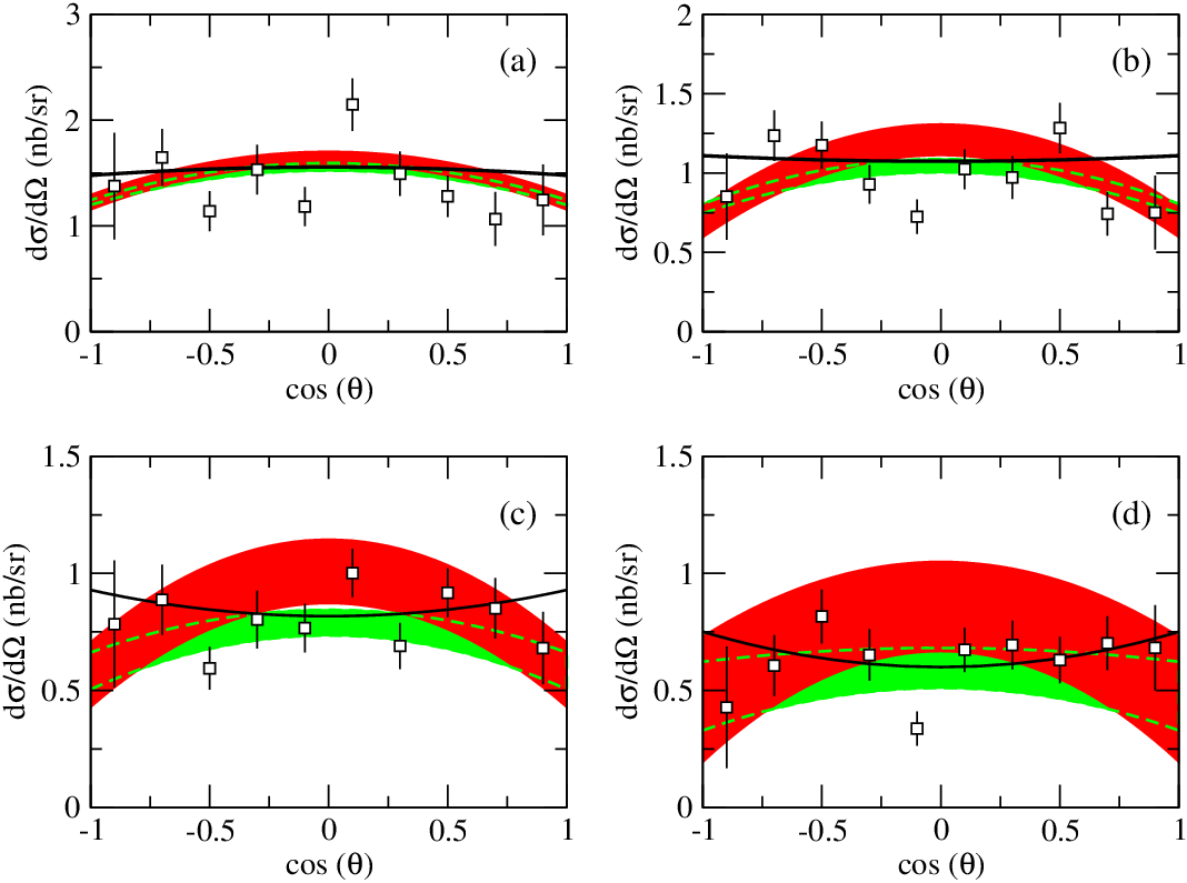
In case of proper differential cross sections were measured, at laboratory momenta of 416, 505, 581, 681, and 888 MeV/c [10]. Also here we restrict ourselves to energies within the range where our EFT interactions are applicable which means we compare our results to the data at the first four momenta only. The corresponding excess energies are 43.5, 62.6, 80.9 and 107.5 MeV, respectively, and pertinent results are presented in Fig. 7. Again there is reasonable agreement of the results based on the EFT interactions with the trend exhibited by the experiment.
Note that in both cases the highest considered energy, MeV ( MeV), is already in a region where our NLO and NNLO interactions no longer reproduce the amplitudes of the PWA sufficiently well, see Fig. 2. Thus, those results may be questionable and they are also afflicted by large uncertainties as reflected by the bands. We show them only for illustrative purposes.
The prediction based on the phenomenological Jülich model disagrees with the trend shown by the BaBar data at the higher energy but is still in line with the PS170 measurement at practically the same excess energy ( MeV). This potential produces a different wave admixture in the amplitude as compared to the EFT interactions – which is not surprising in view of the differences in the corresponding phase shifts, cf. Fig. 2. Obviously, the differential cross sections are more sensitive to details of the interaction than the (energy dependence of the) integrated cross section where the results for all considered interactions more or less coincide. Thus, it would be indeed very valuable to have further data on differential cross sections with improved statistics.
Since our calculation agrees rather well with all measured observables in the near-threshold region it is instructive to consider now predictions for other quantities like spin observables and also for the EMFFs and themselves. Results for the latter are presented in Fig. 8 where we display the modulus and the argument of the ratio as a function of the excess energy. The ratio drops to values slightly below 1 right above the threshold but quickly turns to values larger than 1 with increasing energy. At higher energies the EFT interaction fitted to the PWA and the Jülich meson-exchange model exhibit different trends for the ratio. Again this is simply due to differences in the pertinent amplitudes at these energies, as reflected in the phase shifts shown in Fig. 2. In that figure one can also see that the EFT interaction does not reproduce the phase shifts of the PWA so well anymore for energies above 130 MeV ( 65 MeV). Thus, since the -waves are responsible for the deviation of from 1, one should refrain from associating the results based on our EFT interaction with those implied by the original amplitudes of the PWA at higher energies. In any case, there is also an increasing uncertainty due to the cutoff dependence as visible from the bands.


Predictions for the phase between and are shown in Fig. 8. It is negative over a larger energy range starting from the threshold. Also here the EFT interaction and the Jülich model exhibit a different behavior for higher energies. Overall, the phase remains small with values between 20 degrees.
Finally, let us present some results for spin-dependent observables for the reaction , in particular, for the analyzing power and the spin-correlation parameters . These observables can be written in terms of the () helicity amplitudes given in Eq. (4) following the standard procedure outlined in Refs. [48, 54]:
| (12) |
where . Corresponding expressions in terms of and can be found in Refs. [44, 46, 55, 56]. Our predictions for and at the excess energy MeV are depicted in Figs. 9 and 10, respectively. These observables show clear symmetry properties in case of the one-photon exchange approximation considered here, as one can read off the formulae given in Ref. [46]. Specifically, and are proportional to , and and are proportional to . The magnitudes of and are given by the relative phase of and , namely by Re in case of the former and by Im for the latter [46]. Predictions for these quantities can be found in Fig. 11, again as a function of the excess energy.


Results for spin-dependent observables have been also published by other authors [3, 33, 55, 56, 57] based on various models, however, in general, for much higher energies.
An issue that arises in the context of any observed enhancement in the near-threshold production cross sections or in the corresponding invariant mass spectra is the question whether this is a signal for an bound state. Indeed sometimes it is argued that explanations in terms of FSI effects or via an bound state would mutually exclude each other. This is clearly not the case as we know very well from studies of near-threshold pion production in the reaction [58]. In this case the forces in the and/or final state allow one to achieve a quantitative description of the enhancements seen in the measurements and the very same forces also produce the deuteron bound state in the – partial wave and a virtual state in the . Of course, not every enhancement seen in the experiments is a signal for forces that are strong enough to produce a pole in the near-threshold region. For example, a pronounced near-threshold enhancement was also observed in the invariant mass spectrum as measured in the reaction , see for example [59]. However, evidently there is no near-threshold bound state. Thus, one has to be cautious with conclusions concerning the existence of such bound states from production reactions.
Anyway, let us come back to the interaction investigated here. For the employed EFT potentials a search for poles near the threshold was performed and the results were reported in Ref. [37]. No bound state was found for the – partial wave in the isospin channel. There is a pole in the channel, however, it corresponds to a “binding” energy of MeV, depending on the cutoffs, at NLO and MeV at NNLO [37]. We used quotation marks above because the positive sign of the real part of indicates that these poles are actually located above the threshold. They lie on the physical sheet and, therefore, do not correspond to resonances either. In Ref. [60] such poles are referred to as unstable bound states.
4 Conclusions
We analyzed the reactions and in the near-threshold region with specific emphasis on the role played by the interaction in the initial- or final state. The study is based on the one-photon approximation for the elementary reaction mechanism, but takes into account rigorously the effects of the interaction. For the latter we utilized a recently published potential derived within chiral effective field theory [37] and fitted to results of a new partial-wave analysis of scattering data [36], and also one of the phenomenological meson-exchange models constructed by the Jülich group [21].
Our results confirm the conjecture drawn from previous studies [28, 29, 30, 31, 32, 33, 34, 35] that the pronounced energy dependence of the cross section, seen in pertinent experiments, is indeed primarily due to the interaction. However, the evidence provided now is much more convincing. First the present calculation is technically superior to the earlier ones because it relies on an rigorous treatment of the FSI effects. Secondly, it utilizes amplitudes that have been determined from a PWA. And, finally, by including not only the but also the partial wave the energy dependence of the experimental cross sections can be described quantitatively and over a significantly larger energy region. In addition, even existing data on angular distributions are well reproduced.
Based on our results for the reactions we can produce reliable predictions for the proton electromagnetic form factors and in the timelike region, for near the threshold. The effective proton form factor usually considered in the literature exhibits a strong -dependence for and this behavior is perfectly described by our calculation. The strong -dependence is likewise a consequence of the interaction in the system. For the ratio we predict a non-trivial energy dependence. The ratio drops to values slightly below 1 right above the threshold but turns to values larger than 1 within a couple of MeV. The phase between the form factors, arg, is negative for energies close to the threshold with values in the order of to degrees.
The predictions for the differential cross sections, and also for and arg, based on the chiral EFT interaction and on the phenomenological Jülich potential, show different tendencies with increasing energy. The presently available data (for the differential cross section) are afflicted with sizable uncertainties and, thus, do not allow to discriminate between these differences. Moreover, the BaBar and the PS170 data themselves seem to be incompatible at higher excess energies as visible, for example, in the extracted ratio [12], see also Fig. 8. Therefore, it would be very interesting to perform new measurements of the reactions with improved statistics. As discussed in the review [9], such experiments could be accomplished at the VEPP-2000 accelerator in Novosibirsk [61] or the BEPC-II collider in Beijing (for ), but also by the ANDA set-up at the planned FAIR facility in Darmstadt [62] (for the inverse reaction ). Evidently, aside from pinning down the electromagnetic form factors in the time like region more accurately, such data would also provide further constraints on our knowledge of the elementary interaction where direct information in the near-threshold region is still rather scarce.
Acknowledgements
We would like to thank Kanzo Nakayama for clarifying discussions. This work is supported in part by the DFG and the NSFC through funds provided to the Sino-German CRC 110 “Symmetries and the Emergence of Structure in QCD” and by the EU Integrated Infrastructure Initiative HadronPhysics3.
References
- [1] R. Bijker and F. Iachello, Phys. Rev. C 69, 068201 (2004).
- [2] M. A. Belushkin, H. -W. Hammer and U.-G. Meißner, Phys. Rev. C 75, 035202 (2007).
- [3] A. Z. Dubničková, S. Dubnička and M. Erdelyi, Prog. Part. Nucl. Phys. 61, 162 (2008).
- [4] J. P. B. C. de Melo, T. Frederico, E. Pace, S. Pisano and G. Salme, Phys. Lett. B 671, 153 (2009).
- [5] Y. Yan, K. Khosonthongkee, C. Kobdaj and P. Suebka, J. Phys. G 37, 075007 (2010).
- [6] E. A. Kuraev, E. Tomasi-Gustafsson and A. Dbeyssi, Phys. Lett. B 712, 240 (2012).
- [7] Y. .A. Simonov, Phys. Rev. D 85, 125025 (2012).
- [8] E. L. Lomon and S. Pacetti, Phys. Rev. D 85, 113004 (2012) [Erratum-ibid. D 86, 039901 (2012)].
- [9] A. Denig and G. Salmè, Prog. Part. Nucl. Phys. 68, 113 (2013).
- [10] G. Bardin et al., Nucl. Phys B 411, 3 (1994).
- [11] B. Aubert et al., Phys. Rev. D 73, 012005 (2006).
- [12] J.P. Lees et al., Phys. Rev. D 87, 092005 (2013).
- [13] M. Ablikim et al. [BESIII Collaboration], Phys. Rev. Lett. 108, 112003 (2012).
- [14] B. Aubert et al., Phys. Rev. D 72, 051101 (2005).
- [15] J.Z. Bai et al., Phys. Rev. Lett. 91, 022001 (2003).
- [16] A. Sibirtsev, J. Haidenbauer, S. Krewald, U.-G. Meißner and A.W. Thomas, Phys. Rev. D 71, 054010 (2005).
- [17] B. Loiseau and S. Wycech, Phys. Rev. C 72, 011001 (2005).
- [18] B. Kerbikov, A. Stavinsky, and V. Fedotov, Phys. Rev. C 69, 055205 (2004).
- [19] D.V. Bugg, Phys. Lett. B 598, 8 (2004).
- [20] B.S. Zou and H.C. Chiang, Phys. Rev. D 69, 034004 (2004).
- [21] T. Hippchen, J. Haidenbauer, K. Holinde, V. Mull, Phys. Rev. C 44, 1323 (1991).
- [22] V. Mull, J. Haidenbauer, T. Hippchen, K. Holinde, Phys. Rev. C 44, 1337 (1991).
- [23] V. Mull, K. Holinde, Phys. Rev. C 51, 2360 (1995).
- [24] K.M. Watson, Phys. Rev. 88, 1163 (1952).
- [25] A.B. Migdal, JETP 1, 2 (1955).
- [26] J. Haidenbauer, U.-G. Meißner and A. Sibirtsev, Phys. Rev. D 74, 017501 (2006).
- [27] J. Haidenbauer and U.-G. Meißner, Phys. Rev. D 86, 077503 (2012).
- [28] J. Haidenbauer, H.-W. Hammer, U.-G. Meißner, and A. Sibirtsev, Phys. Lett. B 643, 29 (2006).
- [29] V. F. Dmitriev and A. I. Milstein, Phys. Lett. B 658, 13 (2007).
- [30] G. Y. Chen, H. R. Dong and J. P. Ma, Phys. Rev. D 78, 054022 (2008).
- [31] G. Y. Chen, H. R. Dong and J. P. Ma, Phys. Lett. B 692, 136 (2010).
- [32] O. D. Dalkarov, P. A. Khakhulin and A. Y. Voronin, Nucl. Phys. A 833, 104 (2010).
- [33] A. E. Bondar, V. F. Dmitriev, A. I. Milstein and V. M. Strakhovenko, Phys. Lett. B 697, 159 (2011).
- [34] V. F. Dmitriev and A. I. Milstein, Phys. Lett. B 722, 83 (2013).
- [35] V. F. Dmitriev, A. I. Milstein and S. G. Salnikov, arXiv:1307.0936 [hep-ph].
- [36] D. Zhou and R. G. E. Timmermans, Phys. Rev. C 86, 044003 (2012).
- [37] X.-W. Kang, J. Haidenbauer, U.-G. Meißner, JHEP 1402, 113 (2014).
- [38] P. A. M. Guichon and M. Vanderhaeghen, Phys. Rev. Lett. 91, 142303 (2003).
- [39] P. G. Blunden, W. Melnitchouk and J. A. Tjon, Phys. Rev. Lett. 91, 142304 (2003).
- [40] Y. C. Chen, A. Afanasev, S. J. Brodsky, C. E. Carlson and M. Vanderhaeghen, Phys. Rev. Lett. 93, 122301 (2004).
- [41] M. P. Rekalo and E. Tomasi-Gustafsson, Eur. Phys. J. A 22, 331 (2004).
- [42] M. A. Belushkin, H. -W. Hammer and U.-G. Meißner, Phys. Lett. B 658, 138 (2008).
- [43] J. Arrington, P. G. Blunden and W. Melnitchouk, Prog. Part. Nucl. Phys. 66, 782 (2011).
- [44] G. I. Gakh and E. Tomasi-Gustafsson, Nucl. Phys. A 761, 120 (2005).
- [45] G. I. Gakh and E. Tomasi-Gustafsson, Nucl. Phys. A 771, 169 (2006).
- [46] N.H. Buttimore and E. Jennings, Eur. Phys. J. A 31, 9 (2007).
- [47] N.H. Buttimore and E. Jennings, Eur. Phys. J. A 33, 21 (2007).
- [48] B. Holzenkamp, K. Holinde, J. Speth, Nucl. Phys. A 500, 485 (1989).
- [49] J.G. Körner and M. Kuroda, Phys. Rev. D 16, 2165 (1977).
- [50] R.A. Williams, S. Krewald and K. Linen, Phys. Rev. C 51, 566 (1995).
- [51] E. Epelbaum, W. Glöckle, U.-G. Meißner, Nucl. Phys. A 747, 362 (2005).
- [52] B. Delcourt et al., Phys. Lett. B 86, 395 (1979).
- [53] A. Antonelli et al., Nucl. Phys. B 517, 3 (1998).
- [54] J. Bystricky, F. Lehar, P. Winternitz, J. Physique 39, 1 (1978).
- [55] S. M. Bilenky, C. Giunti and V. Wataghin, Z. Phys. C 59, 475 (1993).
- [56] G. I. Gakh, N. P. Merenkov and E. Tomasi-Gustafsson, Phys. Rev. C 83, 045202 (2011).
- [57] A. Dbeyssi, E. Tomasi-Gustafsson, G. I. Gakh and M. Konchatnyi, Nucl. Phys. A 894, 20 (2012).
- [58] C. Hanhart, Phys. Rept. 397, 155 (2004).
- [59] M. Röder et al. [COSY-TOF Collaboration], Eur. Phys. J. A 49, 157 (2013).
- [60] A. M. Badalian, L. P. Kok, M. I. Polikarpov, Y. A. Simonov, Phys. Rep. 82, 31 (1982).
- [61] E. P. Solodov [CMD3 Collaboration], arXiv:1108.6174 [hep-ex].
- [62] M. Sudol et al., Eur. Phys. J. A 44, 373 (2010).