跳到论文正文
W Papers独立论文阅读器 arXiv:1405.1400 论文正文 计算阅读时间 · 0%
引用这篇论文根据当前论文元数据生成,正式投稿前建议核对。


License: arXiv.org perpetual non-exclusive license
arXiv:1405.1400v2 [stat.ME] 07 May 2014

Multiple Testing of Local Maxima for Detection of Peaks in Random Fields

Dan Cheng*    Armin Schwartzman Note: Partially supported by NIH grant R01-CA157528. The authors thank Alexander Egner of Georg-August-Universität Göttingen for providing the nanoscopy data used in this paper. Affiliation: Department of Statistics, North Carolina State University
Abstract

A topological multiple testing scheme is presented for detecting peaks in images under stationary ergodic Gaussian noise, where tests are performed at local maxima of the smoothed observed signals. The procedure generalizes the one-dimensional scheme of [20] to Euclidean domains of arbitrary dimension. Two methods are developed according to two different ways of computing p-values: (i) using the exact distribution of the height of local maxima [6], available explicitly when the noise field is isotropic; (ii) using an approximation to the overshoot distribution of local maxima above a pre-threshold [6], applicable when the exact distribution is unknown, such as when the stationary noise field is non-isotropic. The algorithms, combined with the Benjamini-Hochberg procedure for thresholding p-values, provide asymptotic strong control of the False Discovery Rate (FDR) and power consistency, with specific rates, as the search space and signal strength get large. The optimal smoothing bandwidth and optimal pre-threshold are obtained to achieve maximum power. Simulations show that FDR levels are maintained in non-asymptotic conditions. The methods are illustrated in a nanoscopy image analysis problem of detecting fluorescent molecules against the image background.

Keywords: Gaussian random field; kernel smoothing; image analysis; overshoot distribution; topological inference; false discovery rate.

1 Introduction

Detection of sparse localized signals embedded in smooth noise is a fundamental problem in image analysis, with applications in many scientific areas such as neuroimaging [26, 13, 24], microscopy [10, 12] and astronomy [5]. The key issue is to find a threshold to determine significant regions. This paper treats the thresholding problem as a multiple testing problem where tests are performed at local maxima of the observed image, allowing error rates and detection power to be topologically defined in terms of detected spatial peaks, rather than pixels or voxels.

Now commonplace in neuroimaging, Keith Worsley pioneered the use of random field theory to approximate the null distribution of the global maximum of the observed image to control the family-wise error rate (FWER) of detected voxels [26, 27, 24]. On the other hand, initial attempts to control the false discovery rate (FDR), desirable for being less conservative, ignored the spatial structure in the data [13]. Recognizing the need to make inferences about connected regions rather than voxels in imaging applications, multiple testing methods have since been developed for pre-defined regions [14, 3, 23] and for the harder problem of detecting unknown clusters [15, 16, 28]. It has been argued, however, that localized signal regions often present themselves as peaks in the image intensity profile, inviting a more powerful analysis based on local maxima of the observed data as the features of interest [17, 7].

Schwartzman et al. [20] formalized peak detection by introducing a multiple testing paradigm where local maxima of the smoothed data are tested for significance. That work, however, was limited to one-dimensional spatial and temporal domains because the distribution of the height of local maxima, a key ingredient for calculation of p-values, has historically been known in closed-form only for one-dimensional stationary Gaussian processes [9]. Recently, Cheng and Schwartzman [6] have obtained exact expressions for the height distribution of isotropic Gaussian fields and an approximation to the overshoot distribution of local maxima of constant-variance Gaussian fields by applying techniques from random matrix theory [11]. These crucial developments allow us in the current paper to extend the multiple testing method of [20] to Euclidean domains of higher dimension.

Our general algorithm consists of the following steps:

  1. (1)

    Kernel smoothing: to increase SNR [25, 22].

  2. (2)

    Candidate peaks: find local maxima of the smoothed field above a pre-threshold.

  3. (3)

    P-values: computed at each local maximum under the complete null hypothesis of no signal anywhere.

  4. (4)

    Multiple testing: apply a multiple testing procedure and declare as detected peaks those local maxima whose p-values are significant.

The main conceptual difference with the algorithm of Schwartzman et al. [20], in addition to being multi-dimensional, is the introduction of a height pre-threshold in step (2). Pre-thresholding is often used in neuroimaging [28] to reduce the number of candidate peaks or regions. Considered formally here, it leads to two ways of applying the above algorithm. If the exact distribution of the height of local maxima for computing p-values in step (3) is known, such as for isotropic fields [6], it is shown here that it is best not to apply pre-thresholding at all. However, if the distribution is unknown, as is the case to date for non-isotropic fields, then pre-thresholding is still valuable in that it enables the use of an approximation of the overshoot distribution of local maxima instead [6]. In step (4), for concreteness, we focus on the Benjamini-Hochberg (BH) procedure [4] for controlling FDR, although other procedures and error criteria could be used. The algorithm is illustrated by a toy example in Figure 1.

Refer to caption Refer to caption Refer to caption
— μ⁡(t)\mu(t) (signal) —z⁡(t)z(t) (noise) —y⁡(t)=μ⁡(t)+z⁡(t)y(t)=\mu(t)+z(t)
Refer to caption Refer to caption Refer to caption
—yγ​(t)y_{\gamma}(t) —candidate peaks —significant peaks
Figure 1: Raw signal μ⁡(t)\mu(t) with six true peaks of different shapes and simulated Gaussian noise z⁡(t)z(t) produce the observed field y⁡(t)y(t) and smoothed field yγ​(t)y_{\gamma}(t). Out of 77 local maxima of yγ​(t)y_{\gamma}(t) (candidate peaks), the BH detection threshold at FDR level 0.2 selects six (significant peaks), one of which is a false positive. In this case, five out of six true peaks are detected.

Following the reasoning of Schwartzman et al. [20], it is shown here that if the noise field is stationary and ergodic, then the proposed algorithm with the BH procedure provides asymptotic control of FDR and power consistency as both the search domain and the signal strength get large, the latter needing to grow only faster than the square root of the log of the former. The large domain assumption helps resolve an interesting aspect of inference for local maxima, namely the fact that the number of tests, equal to the number of observed local maxima, is random. The multiple testing literature usually assumes that the number of tests is fixed. The large domain assumption implies that, by ergodicity, the number of tests behaves asymptotically as its expectation. On the other hand, the strong signal assumption asymptotically eliminates the false positives caused by the smoothed signal spreading into the null regions, causing each signal peak region to be represented by only one observed local maximum within the true domain with probability tending to one. Simulations show that FDR levels are maintained and high power is achieved at finite search domains and moderate signal strength. We also find that the optimal smoothing kernel is approximately that which is closest in shape and bandwidth to the signal peaks to be detected, akin to the matched filter theorem in signal processing [18, 21]. This bandwidth is much larger than the usual optimal bandwidth in nonparametric regression.

The results in this paper supercede those of Schwartzman et al. [20] in the sense that they can be seen as special cases when the domain is of one dimension and no pre-thresholding is applied. In addition, this paper provides specific rates for the asymptotic results, not available in Schwartzman et al. [20], as well as a more rigorous discussion of the optimal smoothing bandwidth. Furthermore, the new concept of approximating p-values by pre-thresholding is not only useful in solving the multi-dimensional problem in this paper but it provides a potentially powerful tool for detection of peaks in non-stationary Gaussian fields on Euclidean space or manifolds [6].

The data analysis and all simulations were implemented in Matlab.

2 The multiple testing scheme

2.1 The model

Consider the signal-plus-noise model

y⁡(t)=μ⁡(t)+z⁡(t),t∈ℝNy(t)=\mu(t)+z(t),\qquad t\in\mathbb{R}^{N} (1)

where the signal μ⁡(t)\mu(t) is composed of unimodal positive peaks of the form

μ⁡(t)=∑j=−∞∞aj​hj​(t),aj>0,\mu(t)=\sum_{j=-\infty}^{\infty}a_{j}h_{j}(t),\qquad a_{j}>0, (2)

and the peak shape hj​(t)≥0h_{j}(t)\geq 0 has compact connected support Sj={t:hj​(t)>0}S_{j}=\{t:h_{j}(t)>0\} and unit action ∫Sjhj​(t)​𝑑t=1\int_{S_{j}}h_{j}(t)\,dt=1 for each jj. Let wγ​(t)≥0w_{\gamma}(t)\geq 0 with bandwidth barameter γ>0\gamma>0 be a unimodal kernel with compact connected support and unit action. Convolving the process (1) with the kernel wγ​(t)w_{\gamma}(t) results in the smoothed random field

yγ​(t)=wγ​(t)∗y⁡(t)=∫ℝNwγ​(t−s)​y​(s)​𝑑s=μγ​(t)+zγ​(t),y_{\gamma}(t)=w_{\gamma}(t)*y(t)=\int_{\mathbb{R}^{N}}w_{\gamma}(t-s)y(s)\,ds=\mu_{\gamma}(t)+z_{\gamma}(t), (3)

where the smoothed signal and smoothed noise are defined as

μγ​(t)=wγ​(t)∗μ⁡(t)=∑j=−∞∞aj​hj,γ​(t),zγ​(t)=wγ​(t)∗z⁡(t).\mu_{\gamma}(t)=w_{\gamma}(t)*\mu(t)=\sum_{j=-\infty}^{\infty}a_{j}h_{j,\gamma}(t),\qquad z_{\gamma}(t)=w_{\gamma}(t)*z(t). (4)

The smoothed noise zγ​(t)z_{\gamma}(t) defined by (3) and (4) is assumed to be a zero-mean thrice differentiable stationary Gaussian field such that for any non-negative integers k1,…,kNk_{1},\ldots,k_{N} with ∑i=1Nki=k∈{0,1,2,3,4}\sum_{i=1}^{N}k_{i}=k\in\{0,1,2,3,4\},

∫ℝ+N|∂krγ​(t)∂t1k1⋯∂tNkN|​𝑑t<∞,\int_{\mathbb{R}_{+}^{N}}\left|\frac{\partial^{k}r_{\gamma}(t)}{\partial t_{1}^{k_{1}}\cdots\partial t_{N}^{k_{N}}}\right|dt<\infty, (5)

where ℝ+N=[0,∞)N\mathbb{R}_{+}^{N}=[0,\infty)^{N} and rγ​(t)=E⁡[zγ​(t)​zγ​(0)]r_{\gamma}(t)={\rm E}[z_{\gamma}(t)z_{\gamma}(0)]. The technical condition (5) is needed for obtaining the rates of FDR control and power consistency below, and by taking k=0k=0, it implies the ergodicity of zγ​(t)z_{\gamma}(t) [9]. It requires that the derivatives of the covariance function of the smoothed field zγ​(t)z_{\gamma}(t) should not decay too slowly. This can be easily obtained by using a Gaussian kernel wγ​(t)w_{\gamma}(t) in (3), regardless of the smoothness of the original noise.

For each jj, the smoothed peak shape hj,γ​(t)=wγ​(t)∗hj​(t)≥0h_{j,\gamma}(t)=w_{\gamma}(t)*h_{j}(t)\geq 0 is unimodal and has compact connected support Sj,γS_{j,\gamma} and unit action. For each jj, we require that hj,γ​(t)h_{j,\gamma}(t) is twice differentiable in the interior of Sj,γS_{j,\gamma} and has no other critical points within its support. For simplicity, the theory requires that the supports Sj,γS_{j,\gamma} do not overlap although this is not crucial in practice.

Let τj\tau_{j} be the unique point in the signal domain Sj,γS_{j,\gamma} where the peak shape hj,γ​(t)h_{j,\gamma}(t) attains its maximum. We impose additionally the following uniformity assumptions on the signal in our model.

  1. (1)

    supj|Sj,γ|<∞\sup_{j}|S_{j,\gamma}|<\infty and infjMj>0\inf_{j}M_{j}>0, where Mj=hj,γ​(τj)M_{j}=h_{j,\gamma}(\tau_{j}).

  2. (2)

    There exists a universal δ>0\delta>0 such that Ijmode:={t∈ℝN:‖t−τj‖≤δ}⊂SjI_{j}^{\rm mode}:=\{t\in\mathbb{R}^{N}:\|t-\tau_{j}\|\leq\delta\}\subset S_{j} for all jj, C=infjCj>0C=\inf_{j}C_{j}>0 and D=infjDj>0D=\inf_{j}D_{j}>0, where

    Cj=inft∈Ijside⟨∇hj,γ(t),(τj−t)/∥τj−t∥⟩,Ijside=Sj,γ\Ijmode,Dj=−supt∈Ijmodesup‖x‖=1xT∇2hj,γ(t)x.\begin{split}C_{j}&=\inf_{t\in I_{j}^{\rm side}}{\langle}\nabla h_{j,\gamma}(t),(\tau_{j}-t)/\|\tau_{j}-t\|\rangle,\quad I_{j}^{\rm side}=S_{j,\gamma}\backslash I_{j}^{\rm mode},\\ D_{j}&=-\sup_{t\in I_{j}^{\rm mode}}\sup_{\|x\|=1}x^{T}\nabla^{2}h_{j,\gamma}(t)x.\end{split}

Here ∇f\nabla f and ∇2f\nabla^{2}f denote the gradient and Hessian of a real-valued function ff, respectively.

Assumption (1) indicates that the sizes of the supports Sj,γS_{j,\gamma} are bounded and that the heights of the peaks of hj,γh_{j,\gamma} are uniformly positive. Assumption (2) indicates that, uniformly for all jj, hj,γ​(t)h_{j,\gamma}(t) increases toward the mode τj\tau_{j} along the direction (τj−t)/‖τj−t‖(\tau_{j}-t)/\|\tau_{j}-t\|, and that sup‖x‖=1xT​∇2hj,γ​(t)​x\sup_{\|x\|=1}x^{T}\nabla^{2}h_{j,\gamma}(t)x, which is the largest eigenvalue of matrix ∇2hj,γ​(t)\nabla^{2}h_{j,\gamma}(t), is strictly negative in the vicinity of the mode so that the peak shape is strictly concave there.

2.2 The STEM algorithm

Suppose we observe y⁡(t)y(t) defined by (1) in the cube of length LL centered at the origin, denoted by U(L)=(−L/2,L/2)NU(L)=(-L/2,L/2)^{N}, and suppose it contains JJ peaks. We call the following procedure STEM (Smoothing and TEsting of Maxima).

Algorithm 1 (STEM algorithm).
  1. (1)

    Kernel smoothing: Construct the field (3), ignoring the effects on the boundary of U⁡(L)U(L).

  2. (2)

    Candidate peaks: For a fixed pre-threshold v∈[−∞,∞)v\in[-\infty,\infty), find the set of local maxima exceeding level vv for yγ​(t)y_{\gamma}(t) in U⁡(L)U(L)

    T~(v)={t∈U(L):yγ(t)>v,∇yγ(t)=0,∇2yγ(t)≺0},\tilde{T}(v)=\left\{t\in U(L):\ y_{\gamma}(t)>v,\ \nabla y_{\gamma}(t)=0,\ \nabla^{2}y_{\gamma}(t)\prec 0\right\}, (6)

    where ∇2yγ​(t)≺0\nabla^{2}y_{\gamma}(t)\prec 0 means that the Hessian matrix is negative definite.

  3. (3)

    P-values: For each t∈T~​(v)t\in\tilde{T}(v), compute the p-value pγ​(t,v)p_{\gamma}(t,v) for testing the (conditional) hypothesis

    ℋ0​(t):μ⁡(t)=0vs.ℋA​(t):μ⁡(t)>0,t∈T~​(v).\mathcal{H}_{0}(t):\ \mu(t)=0\quad\text{vs.}\quad\mathcal{H}_{A}(t):\ \mu(t)>0,\qquad t\in\tilde{T}(v).
  4. (4)

    Multiple testing: Let m~(v)=#{t∈T~(v)}\tilde{m}(v)=\#\{t\in\tilde{T}(v)\} be the number of tested hypotheses. Apply a multiple testing procedure on the set of m~​(v)\tilde{m}(v) p-values {pγ​(t,v),t∈T~​(v)}\{p_{\gamma}(t,v),\,t\in\tilde{T}(v)\}, and declare significant all local maxima whose p-values are smaller than the significance threshold.

When v=−∞v=-\infty, we regard T~=T~​(−∞)\tilde{T}=\tilde{T}(-\infty) as the set of local maxima of yγ​(t)y_{\gamma}(t) in U⁡(L)U(L). In such case, Algorithm 1 becomes an NN-dimensional version of the STEM algorithm proposed in [20] for one-dimensional domains. When v>−∞v>-\infty, an option not available in [20], Algorithm 1 provides a different way of selecting candidate peaks and computing p-values by choosing a pre-threshold vv. In particular, this provides an efficient way to approximate the p-values for stationary and non-isotropic Gaussian noise (Section 4).

Steps (1) and (2) above are well defined under the model assumptions. Step (3) is detailed in Sections 3 and 4 below. For step (4), we use the BH procedure to control FDR (Section 3.2). Notice that, in contrast to the usual BH procedures, the number of tests m~​(v)\tilde{m}(v) is random.

2.3 Error definitions

As in [20], because the location of truly detected peaks may shift as a result of noise, we define a significant local maximum to be a true positive if it falls anywhere inside the support of a true peak. Conversely, we define it to be a false positive if it falls outside the support of any true peak.

Assuming the model of Section 2.1, define the signal region 𝕊1=∪j=1JSj\mathbb{S}_{1}=\cup_{j=1}^{J}S_{j} and null region 𝕊0=U⁡(L)∖𝕊1\mathbb{S}_{0}=U(L)\setminus\mathbb{S}_{1}. For a significance threshold uu above the pre-threshold vv, the total number of detected peaks and the number of falsely detected peaks are

R(u)=#{t∈T~(u)}andV(u)=#{t∈T~(u)∩𝕊0}R(u)=\#\{t\in\tilde{T}(u)\}\quad{\rm and}\quad V(u)=\#\{t\in\tilde{T}(u)\cap\mathbb{S}_{0}\} (7)

respectively. Both are defined as zero if T~​(u)\tilde{T}(u) is empty. The FDR is defined as the expected proportion of falsely detected peaks

FDR⁡(u)=E​{V⁡(u)R⁡(u)∨1}.{\rm FDR}(u)={\rm E}\left\{\frac{V(u)}{R(u)\vee 1}\right\}. (8)

Kernel smoothing enlarges the signal support and increases the probability of obtaining false positives in the null regions neighboring the signal [16]. Define the smoothed signal region 𝕊1,γ=∪j=1JSj,γ⊃𝕊1\mathbb{S}_{1,\gamma}=\cup_{j=1}^{J}S_{j,\gamma}\supset\mathbb{S}_{1} and smoothed null region 𝕊0,γ=U⁡(L)∖𝕊1,γ⊂𝕊0\mathbb{S}_{0,\gamma}=U(L)\setminus\mathbb{S}_{1,\gamma}\subset\mathbb{S}_{0}. We call the difference between the expanded signal support and the true signal support the transition region 𝕋γ=𝕊1,γ∖𝕊1=𝕊0∖𝕊0,γ=∪j=1JTj,γ\mathbb{T}_{\gamma}=\mathbb{S}_{1,\gamma}\setminus\mathbb{S}_{1}=\mathbb{S}_{0}\setminus\mathbb{S}_{0,\gamma}=\cup_{j=1}^{J}T_{j,\gamma}, where Tj,γ=Sj,γ∖SjT_{j,\gamma}=S_{j,\gamma}\setminus S_{j} is the transition region corresponding to each peak jj.

In general, more than one significant local maximum may be obtained within the domain of a true peak, affecting the interpretation of definition (8). However, this has no effect asymptotically because each true peak is represented by exactly one local maximum of the smoothed observed field with probability tending to 1 (Lemma 9 in Section 7.1).

2.4 Power

We define the power of Algorithm 1 as the expected fraction of true discovered peaks

Power(u)=E(1J∑j=1J𝟙{T~(u)∩Sj≠∅})=1J∑j=1JPowerj(u),{\rm Power}(u)={\rm E}\left(\frac{1}{J}\sum_{j=1}^{J}\mathbbm{1}_{\left\{\tilde{T}(u)\cap S_{j}\neq\emptyset\right\}}\right)=\frac{1}{J}\sum_{j=1}^{J}{\rm Power}_{j}(u), (9)

where Powerj​(u){\rm Power}_{j}(u) is the probability of detecting peak jj

Powerj​(u)=P⁡(T~​(u)∩Sj≠∅).{\rm Power}_{j}(u)={\rm P}\left(\tilde{T}(u)\cap S_{j}\neq\emptyset\right). (10)

The indicator function in (9) ensures that only one significant local maximum is counted within the same peak support, so power is not inflated. Again, this has no effect asymptotically because each true peak is represented by exactly one local maximum of the smoothed observed process with probability tending to 1 (Lemma 9 in Section 7.1).

3 Detection of peaks by the height distribution of local maxima

3.1 P-values

Given the observed heights yγ​(t)y_{\gamma}(t) at the local maxima t∈T~​(v)t\in\tilde{T}(v), the p-values in step (3) of Algorithm 1 are computed as pγ​(t,v)=Fγ​(yγ​(t),v)p_{\gamma}(t,v)=F_{\gamma}\left(y_{\gamma}(t),v\right), t∈T~​(v)t\in\tilde{T}(v), where

Fγ​(u,v)=P⁡(zγ​(t)>u|t∈T~​(v))F_{\gamma}(u,v)={\rm P}\left(z_{\gamma}(t)>u~\Big|~t\in\tilde{T}(v)\right) (11)

denotes the right tail probability of zγ​(t)z_{\gamma}(t) at the local maximum t∈T~​(v)t\in\tilde{T}(v), evaluated under the complete null hypothesis μ⁡(t)=0,∀t\mu(t)=0,\forall t. By convention, when v=−∞v=-\infty, denote

Fγ​(u)=Fγ​(u,−∞).F_{\gamma}(u)=F_{\gamma}(u,-\infty). (12)

The conditional distribution (11) is a Palm distribution [2, Ch. 6] and requires careful evaluation because the conditioning event has probability zero. Unlike the marginal distribution of zγ​(t)z_{\gamma}(t), it is not Gaussian but stochastically greater. Generally, for a constant-variance Gaussian field, there is an implicit formula for Fγ​(⋅,v)F_{\gamma}(\cdot,v) [6]. Theorem 2 below ([6], [2]) provides the formula for Fγ​(⋅,v)F_{\gamma}(\cdot,v) for stationary Gaussian fields.

Let σγ2=Var⁡(zγ​(t))\sigma_{\gamma}^{2}={\rm Var}(z_{\gamma}(t)) and Λγ=Cov⁡(∇zγ​(t))\Lambda_{\gamma}={\rm Cov}(\nabla z_{\gamma}(t)), both independent of tt due to the stationarity of zγ​(t)z_{\gamma}(t). Denote by m~0,γ​(U​(1))\tilde{m}_{0,\gamma}(U(1)) and m~0,γ​(U​(1),u)\tilde{m}_{0,\gamma}(U(1),u) respectively the number of local maxima of zγ​(t)z_{\gamma}(t) and the number of local maxima of zγ​(t)z_{\gamma}(t) exceeding level uu in the unit cube U(1)=(−1/2,1/2)NU(1)=(-1/2,1/2)^{N}. In fact, m~0,γ​(U⁡(1))=m~0,γ​(U⁡(1),−∞)\tilde{m}_{0,\gamma}(U(1))=\tilde{m}_{0,\gamma}(U(1),-\infty). By the Kac-Rice formula [1],

E[m~0,γ​(U​(1),u)]=E[|det∇2zγ(t)|𝟙{zγ(t)>u}𝟙{∇2zγ(t)≺0}|∇zγ(t)=0]p∇zγ​(t)(0),\begin{split}{\rm E}&[\tilde{m}_{0,\gamma}(U(1),u)]\\ &={\rm E}\left[|{\rm det}\nabla^{2}z_{\gamma}(t)|\mathbbm{1}_{\{z_{\gamma}(t)>u\}}\mathbbm{1}_{\{\nabla^{2}z_{\gamma}(t)\prec 0\}}\big|\nabla z_{\gamma}(t)=0\right]p_{\nabla z_{\gamma}(t)}(0),\end{split} (13)

where p∇zγ​(t)(0)=(2π)−N/2(det(Λγ))−1/2p_{\nabla z_{\gamma}(t)}(0)=(2\pi)^{-N/2}({\rm det}(\Lambda_{\gamma}))^{-1/2} is the density function of ∇zγ​(t)\nabla z_{\gamma}(t) evaluated at 00.

Theorem 2.

Suppose the assumptions of Section 2.1 hold and that μ⁡(t)=0,∀t\mu(t)=0,\forall t. Then the distributions (11) and (12) are given respectively by

Fγ​(u,v)=E⁡[m~0,γ​(U⁡(1),u)]E⁡[m~0,γ​(U⁡(1),v)]a​n​dFγ​(u)=E⁡[m~0,γ​(U⁡(1),u)]E​[m~0,γ​(U​(1))].F_{\gamma}(u,v)=\frac{{\rm E}[\tilde{m}_{0,\gamma}(U(1),u)]}{{\rm E}[\tilde{m}_{0,\gamma}(U(1),v)]}\quad{\text{a}nd}\quad F_{\gamma}(u)=\frac{{\rm E}[\tilde{m}_{0,\gamma}(U(1),u)]}{{\rm E}[\tilde{m}_{0,\gamma}(U(1))]}.

It should be mentioned that the expectations above involving the indicator function 𝟙{∇2zγ(t)≺0}\mathbbm{1}_{\{\nabla^{2}z_{\gamma}(t)\prec 0\}} are extremely hard to compute. Therefore, the explicit formula for FγF_{\gamma} is usually unknown. The only exception, as far as we know, is the case when the field zγz_{\gamma} is isotropic. This is because, in such case, one may apply the Gaussian Orthogonal Ensemble (GOE) technique from random matrix theory to compute these expectations [11]. The corresponding explicit formula for FγF_{\gamma} for isotropic Gaussian fields was recently obtained in [6, Theorem 2.14]. This will be used to compute the p-values exactly, see Proposition 6 below.

3.2 Error control and power consistency

Suppose the BH procedure is applied in step (4) of Algorithm 1, as follows. For a fixed α∈(0,1)\alpha\in(0,1), let kk be the largest index for which the iith smallest p-value is less than i​α/m~​(v)i\alpha/\tilde{m}(v). Then the null hypothesis ℋ0​(t)\mathcal{H}_{0}(t) at t∈T~​(v)t\in\tilde{T}(v) is rejected if

pγ(t,v)<k​αm~​(v)⇔yγ(t)>u~BH(v)=Fγ(⋅,v)−1(k​αm~​(v)),p_{\gamma}(t,v)<\frac{k\alpha}{\tilde{m}(v)}\quad\iff\quad y_{\gamma}(t)>\tilde{u}_{{\rm BH}}(v)=F_{\gamma}(\cdot,v)^{-1}\left(\frac{k\alpha}{\tilde{m}(v)}\right), (14)

where k​α/m~​(v)k\alpha/\tilde{m}(v) is defined as 1 if m~​(v)=0\tilde{m}(v)=0. Since u~BH​(v)\tilde{u}_{{\rm BH}}(v) is random, definition (8) is hereby modified to

FDRBH​(v)=E⁡{V​(u~BH​(v))R​(u~BH​(v))∨1},{\rm FDR}_{{\rm BH}}(v)={\rm E}\left\{\frac{V(\tilde{u}_{{\rm BH}}(v))}{R(\tilde{u}_{{\rm BH}}(v))\vee 1}\right\}, (15)

where R⁡(⋅)R(\cdot) and V⁡(⋅)V(\cdot) are defined in (7) and the expectation is taken over all possible realizations of the random threshold u~BH​(v)\tilde{u}_{{\rm BH}}(v).

Define the conditions:

  1. (C1)

    The assumptions of Section 2.1 hold.

  2. (C2)

    L→∞L\to\infty and a=infjaj→∞a=\inf_{j}a_{j}\to\infty, such that (log⁡L)/a2→0(\log L)/a^{2}\to 0, J/LN=A1+O(a−2+L−N/2)J/L^{N}=A_{1}+O(a^{-2}+L^{-N/2}) and |𝕊1,γ|/LN=A2,γ+O(a−2+L−N/2)|\mathbb{S}_{1,\gamma}|/L^{N}=A_{2,\gamma}+O(a^{-2}+L^{-N/2}) with A1>0A_{1}>0 and A2,γ∈[0,1)A_{2,\gamma}\in[0,1).

Theorem 3.

Let conditions (C1) and (C2) hold.

(i) Suppose that Algorithm 1 is applied with a fixed threshold u>vu>v, then

FDR(u)≤E⁡[m~0,γ​(U⁡(1),u)]​(1−A2,γ)E⁡[m~0,γ​(U⁡(1),u)]​(1−A2,γ)+A1+O(a−2+L−N/2).{\rm FDR}(u)\leq\frac{{\rm E}[\tilde{m}_{0,\gamma}(U(1),u)](1-A_{2,\gamma})}{{\rm E}[\tilde{m}_{0,\gamma}(U(1),u)](1-A_{2,\gamma})+A_{1}}+O(a^{-2}+L^{-N/2}). (16)

(ii) Suppose that Algorithm 1 is applied with the random threshold u~BH​(v)\tilde{u}_{{\rm BH}}(v) (14), then

FDRBH(v)≤αE⁡[m~0,γ​(U⁡(1),v)]​(1−A2,γ)E⁡[m~0,γ​(U⁡(1),v)]​(1−A2,γ)+A1+O(a−1+L−N/4).{\rm FDR}_{{\rm BH}}(v)\leq\alpha\frac{{\rm E}[\tilde{m}_{0,\gamma}(U(1),v)](1-A_{2,\gamma})}{{\rm E}[\tilde{m}_{0,\gamma}(U(1),v)](1-A_{2,\gamma})+A_{1}}+O(a^{-1}+L^{-N/4}). (17)

The proof of Theorem 3 is given in Section 7.2. It can be seen from the proof of Theorem 3 that the inequalities in (16) and (17) become equalities asymptotically (without specific rates), so the bounds given in (16) and (17) are tight and can be regarded respectively as the asymptotic estimators of FDR⁡(u){\rm FDR}(u) and FDRBH​(v){\rm FDR}_{{\rm BH}}(v). By (37), the random threshold u~BH​(v)\tilde{u}_{{\rm BH}}(v) converges asymptotically to the deterministic threshold

uBH∗​(v)=Fγ−1​(α​A1​E​[m~0,γ​(U⁡(1),v)]/E⁡[m~0,γ​(U⁡(1))]A1+E⁡[m~0,γ​(U⁡(1),v)]​(1−A2,γ)​(1−α)),u^{*}_{{\rm BH}}(v)=F_{\gamma}^{-1}\left(\frac{\alpha A_{1}{\rm E}[\tilde{m}_{0,\gamma}(U(1),v)]/{\rm E}[\tilde{m}_{0,\gamma}(U(1))]}{A_{1}+{\rm E}[\tilde{m}_{0,\gamma}(U(1),v)](1-A_{2,\gamma})(1-\alpha)}\right), (18)

which is a strictly increasing function in vv. The threshold (14) can be viewed as the smallest solution of the equation α​G~​(u,v)≥Fγ​(u,v)\alpha\tilde{G}(u,v)\geq F_{\gamma}(u,v), where G~​(u,v)\tilde{G}(u,v) is the empirical right cumulative distribution function of yγ​(t),t∈T~​(v)y_{\gamma}(t),~t\in\tilde{T}(v) [13]. Taking the limit of that equation as L→∞L\to\infty yields the solution (18).

Similar to the definition of FDRBH{\rm FDR}_{{\rm BH}} (15), since u~BH​(v)\tilde{u}_{{\rm BH}}(v) is random, define

PowerBH(v)=E(1J∑j=1J𝟙{T~(u~BH(v))∩Sj≠∅}).{\rm Power}_{{\rm BH}}(v)={\rm E}\left(\frac{1}{J}\sum_{j=1}^{J}\mathbbm{1}_{\left\{\tilde{T}(\tilde{u}_{{\rm BH}}(v))\cap S_{j}\neq\emptyset\right\}}\right). (19)

Since u~BH​(v)\tilde{u}_{{\rm BH}}(v) converges to the deterministic threshold uBH∗​(v)u^{*}_{{\rm BH}}(v), which attains the minimum at v=−∞v=-\infty, we see that the power is asymptotically maximized at v=−∞v=-\infty when γ\gamma is fixed. This will be reflected in the simulation studies below (Figure 3) and it shows that, if the exact height distribution of local maxima Fγ​(⋅,v)F_{\gamma}(\cdot,v) or Fγ​(⋅)F_{\gamma}(\cdot) is known, for example the smoothed noise zγz_{\gamma} is an isotropic Gaussian field, then we will choose to apply the original STEM algorithm without pre-thresholding (i.e., v=−∞v=-\infty) to perform the test.

The following lemma, whose proof is given in Section 7.3, provides an asymptotic approximation to the power at a fixed threshold.

Lemma 4.

Let conditions (C1) and (C2) hold. As aj→∞a_{j}\to\infty, the power for peak jj (10) can be approximated by

Powerj​(u)=Φ⁡(aj​hj,γ​(τj)−uσγ)​(1+O⁡(aj−2)).{\rm Power}_{j}(u)=\Phi\left(\frac{a_{j}h_{j,\gamma}(\tau_{j})-u}{\sigma_{\gamma}}\right)(1+O(a_{j}^{-2})). (20)

The next result indicates that the BH procedure is asymptotically consistent. The proof is given in Section 7.3.

Theorem 5.

Let conditions (C1) and (C2) hold.

(i) Suppose that Algorithm 1 is applied with a fixed threshold uu, then

Power⁡(u)=1−O⁡(a−2).{\rm Power}(u)=1-O(a^{-2}).

(ii) Suppose that Algorithm 1 is applied with the random threshold u~BH​(v)\tilde{u}_{{\rm BH}}(v) (14), then

PowerBH(v)=1−O(a−2+L−N/2).{\rm Power}_{{\rm BH}}(v)=1-O(a^{-2}+L^{-N/2}).

The results in Theorem 5 rely on the condition (log⁡L)/a2→0(\log L)/a^{2}\to 0 in (C2). If this condition is not satisfied, then it can be seen from the proofs of Lemmas 4 and 11 below that the power may be bounded above by a constant strictly less than one.

3.3 Optimal smoothing kernel

The best smoothing kernel wγ​(t)w_{\gamma}(t) is that which maximizes the detection power under the true model. By Lemma 4, the power (20) is approximately maximized by maximizing the signal-to-noise ratio (SNR)

SNRj,γ=aj​hj,γ​(τj)σγ=aj​∫ℝNwγ​(s)​hj​(s)​𝑑sσ​∫ℝNwγ2​(s)​𝑑s,{\rm SNR}_{j,\gamma}=\frac{a_{j}h_{j,\gamma}(\tau_{j})}{\sigma_{\gamma}}=\frac{a_{j}\int_{\mathbb{R}^{N}}w_{\gamma}(s)h_{j}(s)\,ds}{\sigma\sqrt{\int_{\mathbb{R}^{N}}w^{2}_{\gamma}(s)\,ds}}, (21)

where σ\sigma is the standard deviation of the observed process y⁡(t)y(t). The smoothing kernel wγ​(t)w_{\gamma}(t) that maximizes (21) is called a matched filter in signal processing [18, 21]. It is known in signal processing that if the peak locations are known, then the matched filter maximizes the detection power exactly. As shown in the simulations, the result only holds approximately in our case because the peak locations are unknown.

3.4 Isotropic Gaussian fields

The following result gives an explicit expression for the distribution (11) in the special case when N=2N=2 and the noise field zγ​(t)z_{\gamma}(t) is isotropic. It is obtained from [6, Example 2.16] by standardizing the field in (11) as Fγ​(u,v)=P⁡(zγ​(t)/σγ>u/σγ|t∈T~​(v))F_{\gamma}(u,v)={\rm P}(z_{\gamma}(t)/\sigma_{\gamma}>u/\sigma_{\gamma}|t\in\tilde{T}(v)). Here, denote by ϕ⁡(x)\phi(x) and Φ⁡(x)\Phi(x) respectively the density function and cumulative distribution function (cdf) of the standard Gaussian distribution.

Proposition 6.

Let the assumptions in Theorem 2 hold and let zγ​(t)z_{\gamma}(t) be an isotropic Gaussian field over ℝ2\mathbb{R}^{2} with correlation function

ργ​(‖t−s‖2)=E⁡[zγ​(t)​zγ​(s)]/σγ2\rho_{\gamma}(\|t-s\|^{2})={\rm E}[z_{\gamma}(t)z_{\gamma}(s)]/\sigma_{\gamma}^{2}

and ργ′′−ργ′2≥0\rho_{\gamma}^{\prime\prime}-\rho_{\gamma}^{\prime 2}\geq 0, where ργ′=ργ′​(0)\rho_{\gamma}^{\prime}=\rho_{\gamma}^{\prime}(0) and ργ′′=ργ′′​(0)\rho_{\gamma}^{\prime\prime}=\rho_{\gamma}^{\prime\prime}(0). Let κγ=−ργ′/ργ′′\kappa_{\gamma}=-\rho_{\gamma}^{\prime}/\sqrt{\rho_{\gamma}^{\prime\prime}}, then E[m~0,γ(U(1))]=−3ργ′′/(3πργ′){\rm E}[\tilde{m}_{0,\gamma}(U(1))]=-\sqrt{3}\rho_{\gamma}^{\prime\prime}/(3\pi\rho_{\gamma}^{\prime}) and the distributions (12) and (11) are given respectively by Fγ​(u)=∫u/σγ∞gγ​(x)​𝑑xF_{\gamma}(u)=\int_{u/\sigma_{\gamma}}^{\infty}g_{\gamma}(x)dx and Fγ​(u,v)=Fγ​(u)/Fγ​(v)F_{\gamma}(u,v)=F_{\gamma}(u)/F_{\gamma}(v), where

gγ​(x)=3​κγ2​(x2−1)​ϕ​(x)​Φ​(κγ​x2−κγ2)+κγ​x​3​(2−κγ2)2​π​e−x22−κγ2+6π⁡(3−κγ2)​e−3​x22​(3−κγ2)​Φ​(κγ​x(3−κγ2)​(2−κγ2)).\begin{split}g_{\gamma}(x)&=\sqrt{3}\kappa_{\gamma}^{2}(x^{2}-1)\phi(x)\Phi\left(\frac{\kappa_{\gamma}x}{\sqrt{2-\kappa_{\gamma}^{2}}}\right)+\frac{\kappa_{\gamma}x\sqrt{3(2-\kappa_{\gamma}^{2})}}{2\pi}e^{-\frac{x^{2}}{2-\kappa_{\gamma}^{2}}}\\ &\quad+\frac{\sqrt{6}}{\sqrt{\pi(3-\kappa_{\gamma}^{2})}}e^{-\frac{3x^{2}}{2(3-\kappa_{\gamma}^{2})}}\Phi\left(\frac{\kappa_{\gamma}x}{\sqrt{(3-\kappa_{\gamma}^{2})(2-\kappa_{\gamma}^{2})}}\right).\end{split}

As shown in [6],

ργ′=−12​σγ2​Var​(∂zγ​(t)∂ti),ργ′′=112​σγ2​Var​(∂2zγ​(t)∂ti2)\rho_{\gamma}^{\prime}=-\frac{1}{2\sigma_{\gamma}^{2}}{\rm Var}\left(\frac{\partial z_{\gamma}(t)}{\partial t_{i}}\right),\quad\rho_{\gamma}^{\prime\prime}=\frac{1}{12\sigma_{\gamma}^{2}}{\rm Var}\left(\frac{\partial^{2}z_{\gamma}(t)}{\partial t_{i}^{2}}\right)

for any i=1,…,Ni=1,\ldots,N. Therefore, in order to estimate ργ′\rho_{\gamma}^{\prime} and ργ′′\rho_{\gamma}^{\prime\prime}, we only need to estimate the variances of the derivatives of zγz_{\gamma} (or equivalently yγy_{\gamma}).

Example 7 (Gaussian autocorrelation model).

Let the noise z⁡(t)z(t) in (1) be constructed as

z⁡(t)=σ​∫ℝN1νN​ϕN​(t−sν)​𝑑B​(s),σ,ν>0,z(t)=\sigma\int_{\mathbb{R}^{N}}\frac{1}{\nu^{N}}\phi_{N}\left(\frac{t-s}{\nu}\right)\,dB(s),\qquad\sigma,\nu>0,

where ϕN(x)=(2π)−N/2e−∥x∥2/2\phi_{N}(x)=(2\pi)^{-N/2}e^{-\|x\|^{2}/2} for all x∈ℝNx\in\mathbb{R}^{N} is the NN-dimensional standard Gaussian density, d​B​(s)dB(s) is Gaussian white noise and ν>0\nu>0 (z⁡(t)z(t) is regarded by convention as Gaussian white noise when ν=0\nu=0). Convolving with a Gaussian kernel wγ​(t)=(1/γN)​ϕN​(t/γ)w_{\gamma}(t)=(1/\gamma^{N})\phi_{N}(t/\gamma) with γ>0\gamma>0 as in (4) produces a zero-mean infinitely differentiable stationary ergodic Gaussian field

zγ​(t)=wγ​(t)∗z⁡(t)=σ​∫ℝN1ξN​ϕN​(t−sξ)​𝑑B​(s),ξ=γ2+ν2,z_{\gamma}(t)=w_{\gamma}(t)*z(t)=\sigma\int_{\mathbb{R}^{N}}\frac{1}{\xi^{N}}\phi_{N}\left(\frac{t-s}{\xi}\right)\,dB(s),\qquad\xi=\sqrt{\gamma^{2}+\nu^{2}},

with σγ2=σ2/(2N​πN/2​ξN)\sigma_{\gamma}^{2}=\sigma^{2}/(2^{N}\pi^{N/2}\xi^{N}), ργ′=−(2​ξ)−2\rho_{\gamma}^{\prime}=-(2\xi)^{-2}, ργ′′=(2​ξ)−4\rho_{\gamma}^{\prime\prime}=(2\xi)^{-4} and κγ=1\kappa_{\gamma}=1. The above expressions may be used as approximations if the kernel, required to have finite support, is truncated at [−γ​d,γ​d]N[-\gamma d,\gamma d]^{N} for moderately large dd, say d=3d=3.

Suppose the signal peak jj is a truncated Gaussian density

hj(t)=(1/bjN)ϕN[(t−τj)/bj]𝟙{(t−τj)/bj∈[−cj,cj]N},bj,cj>0.h_{j}(t)=(1/b_{j}^{N})\phi_{N}[(t-\tau_{j})/b_{j}]\mathbbm{1}_{\{(t-\tau_{j})/b_{j}\in[-c_{j},c_{j}]^{N}\}},\quad b_{j},c_{j}>0.

Ignoring the truncation, hj,γ​(t)=wγ​(t)∗hj​(t)h_{j,\gamma}(t)=w_{\gamma}(t)*h_{j}(t) in (21) is the convolution of two Gaussian densities with variances γ2\gamma^{2} and bj2b_{j}^{2}, which is another Gaussian density with variance γ2+bj2\gamma^{2}+b_{j}^{2}. We have that

SNRj,γ=aj​hj,γ​(τj)σγ=ajσ​πN/4​[γ2+ν2(γ2+bj2)2]N/4.{\rm SNR}_{j,\gamma}=\frac{a_{j}h_{j,\gamma}(\tau_{j})}{\sigma_{\gamma}}=\frac{a_{j}}{\sigma\pi^{N/4}}\left[\frac{\gamma^{2}+\nu^{2}}{(\gamma^{2}+b_{j}^{2})^{2}}\right]^{N/4}.

As a function of γ\gamma, the SNR is maximized at

argmaxγSNRj,γ={bj2−2​ν2,ν<bj/20,ν>bj/2.\operatornamewithlimits{argmax}_{\gamma}{\rm SNR}_{j,\gamma}=\begin{cases}\sqrt{b_{j}^{2}-2\nu^{2}},&\nu<b_{j}/\sqrt{2}\\ 0,&\nu>b_{j}/\sqrt{2}.\end{cases} (22)

In particular, when ν=0\nu=0, we have that the optimal bandwidth for peak jj is γ=bj\gamma=b_{j}, the same as the signal bandwidth. We show in the simulations below that the optimal γ\gamma is indeed close to (22). It can be seen from (22) that as ν\nu gets larger, which means that y⁡(t)y(t) gets smoother, the optimal γ\gamma becomes smaller. If ν\nu is large enough, there is no need to smooth at all.

4 Detection of peaks by approximated overshoot distribution

4.1 Approximating the overshoot distribution

In the neuroimaging literature, it has been proposed to pre-threshold the test statistic field and then perform the inference on the supra-threshold statistics [28]. We showed theoretically in Section 3.2 and will confirm by simulations that, in the best case scenario where the exact distribution of the height of local maxima is known, pre-thresholding (v=−∞v=-\infty) does not increase detection power. However, pre-thresholding is still very valuable if the exact distribution is unknown but an approximation is known.

As mentioned, if the Gaussian field is only stationary but not isotropic, then the explicit formula for Fγ​(u,v)F_{\gamma}(u,v) (11) is unknown so far. By [6, Corollary 2.7], there exists ε0>0\varepsilon_{0}>0 such that as v→∞v\to\infty and u>vu>v,

Fγ​(u,v)=Kγ​(u,v)​(1+o⁡(e−ε0​v2)),F_{\gamma}(u,v)=K_{\gamma}(u,v)(1+o(e^{-\varepsilon_{0}v^{2}})),

where

Kγ​(u,v)=HN−1(u/σγ)e−u2/(2σγ2)HN−1(v/σγ)e−v2/(2σγ2)K_{\gamma}(u,v)=\frac{H_{N-1}(u/\sigma_{\gamma})e^{-u^{2}/(2\sigma_{\gamma}^{2})}}{H_{N-1}(v/\sigma_{\gamma})e^{-v^{2}/(2\sigma_{\gamma}^{2})}}

and HN−1​(x)H_{N-1}(x) is the Hermite polynomial of order N−1N-1. A similar argument to the proof of [6, Corollary 2.7] yields that for a fixed vv, as u→∞u\to\infty,

Fγ​(u,v)=βγ​(v)​Kγ​(u,v)​(1+o⁡(e−ε0​u2)),F_{\gamma}(u,v)=\beta_{\gamma}(v)K_{\gamma}(u,v)(1+o(e^{-\varepsilon_{0}u^{2}})), (23)

where

βγ​(v)=(2π)−(N+1)/2σγ−N(det(Λγ))1/2HN−1(v/σγ)e−v2/(2σγ2)E⁡[m~0,γ​(U⁡(1),v)]\beta_{\gamma}(v)=\frac{(2\pi)^{-(N+1)/2}\sigma_{\gamma}^{-N}({\rm det(\Lambda_{\gamma})})^{1/2}H_{N-1}(v/\sigma_{\gamma})e^{-v^{2}/(2\sigma_{\gamma}^{2})}}{{\rm E}[\tilde{m}_{0,\gamma}(U(1),v)]} (24)

and Λγ=Cov⁡(∇zγ​(t))\Lambda_{\gamma}={\rm Cov}(\nabla z_{\gamma}(t)). Note that βγ​(v)\beta_{\gamma}(v) is similar to the ratio of the expected Euler characteristic [1, Lemma 11.7.1] and the expected number of local maxima of zγ​(t)z_{\gamma}(t) over the unit cube U⁡(1)U(1). It is conjectured that βγ​(v)<1\beta_{\gamma}(v)<1 for all v>0v>0 (this is true for N=1N=1 and N=2N=2 [6]).

Theorem 8.

Let conditions (C1) and (C2) hold. Suppose that Algorithm 1 is applied with the random threshold u~BH​(v)\tilde{u}_{{\rm BH}}(v) by using Kγ​(u,v)K_{\gamma}(u,v) instead of Fγ​(u,v)F_{\gamma}(u,v) to compute p-values, then as v→∞v\to\infty such that v2/log⁡(L)→0v^{2}/\log(L)\to 0 and v2/log⁡(a)→0v^{2}/\log(a)\to 0,

FDRBH​(v)≤α​E⁡[m~0,γ​(U⁡(1),v)]​(1−A2,γ)​βγ​(v)E⁡[m~0,γ​(U⁡(1),v)]​(1−A2,γ)+A1​(1+o⁡(e−ε0​v2)),{\rm FDR}_{{\rm BH}}(v)\leq\alpha\frac{{\rm E}[\tilde{m}_{0,\gamma}(U(1),v)](1-A_{2,\gamma})\beta_{\gamma}(v)}{{\rm E}[\tilde{m}_{0,\gamma}(U(1),v)](1-A_{2,\gamma})+A_{1}}(1+o(e^{-\varepsilon_{0}v^{2}})), (25)

where ε0>0\varepsilon_{0}>0 is some constant and βγ​(v)\beta_{\gamma}(v) is defined in (24), and moreover,

PowerBH(v)=1−O(a−2+L−N/2).{\rm Power}_{{\rm BH}}(v)=1-O(a^{-2}+L^{-N/2}). (26)

Note that for a fixed threshold uu, the control of FDR⁡(u){\rm FDR}(u) and the consistency of power Power⁡(u){\rm Power}(u) in Theorem 8 will be the same as those given in part (i) of Theorem 3 and part (i) in Theorem 5 respectively. From the proof of Theorem 8, we see that the limit is in fact taken when u→∞u\to\infty while vv is fixed. However, we cannot tell the exact gap between uu and vv, though it is assumed that uu is always greater than vv. It is likely that u~BH​(v)\tilde{u}_{{\rm BH}}(v) or uBH∗⁣∗​(v)u^{**}_{{\rm BH}}(v) (27) below is still relatively large for small vv, which is true when applying the STEM algorithm by using F⁡(⋅,v)F(\cdot,v) to compute p-values. Therefore, in our simulations below (Figure 4), the approximation in Theorem 8 even works well for small vv.

4.2 Optimal pre-threshold

Under the conditions in Theorem 8, by (43), we see that the random threshold u~BH​(v)\tilde{u}_{{\rm BH}}(v) converges asymptotically to the deterministic threshold

uBH∗⁣∗​(v)=Fγ−1​(α​A1​βγ​(v)​E​[m~0,γ​(U⁡(1),v)]/E⁡[m~0,γ​(U⁡(1))]A1+E⁡[m~0,γ​(U⁡(1),v)]​(1−A2,γ)​(1−α​βγ​(v)))​(1+o⁡(1)).u^{**}_{{\rm BH}}(v)=F_{\gamma}^{-1}\left(\frac{\alpha A_{1}\beta_{\gamma}(v){\rm E}[\tilde{m}_{0,\gamma}(U(1),v)]/{\rm E}[\tilde{m}_{0,\gamma}(U(1))]}{A_{1}+{\rm E}[\tilde{m}_{0,\gamma}(U(1),v)](1-A_{2,\gamma})(1-\alpha\beta_{\gamma}(v))}\right)(1+o(1)). (27)

For fixed γ\gamma, the power (20) is maximized at the optimal pre-threshold minimizing uBH∗⁣∗​(v)u^{**}_{{\rm BH}}(v), which is

vopt=argmax𝑣​HN−1(v/σγ)e−v2/(2σγ2)A1+E⁡[m~0,γ​(U⁡(1),v)]​(1−A2,γ)​(1−α​βγ​(v)).v_{\rm opt}=\underset{v}{\operatorname{argmax}}\frac{H_{N-1}(v/\sigma_{\gamma})e^{-v^{2}/(2\sigma_{\gamma}^{2})}}{A_{1}+{\rm E}[\tilde{m}_{0,\gamma}(U(1),v)](1-A_{2,\gamma})(1-\alpha\beta_{\gamma}(v))}. (28)

Let γ\gamma and α\alpha be fixed, we see that voptv_{\rm opt} depends only on the covariance structure of zγ​(t)z_{\gamma}(t).

5 Simulation studies

ν=0\nu=0 ν=1\nu=1 ν=2\nu=2

———–FDR

Refer to caption Refer to caption Refer to caption

———–Power

Refer to caption Refer to caption Refer to caption
—γ\gamma —γ\gamma —γ\gamma
Figure 2: Realized (black) and “theoretical” (blue) FDR, Realized (black) and “theoretical” (blue) power of the BH procedure by the exact height distribution FγF_{\gamma} (i.e., v=−∞v=-\infty) for a=55a=55 (solid), a=45a=45 (dashed) and a=35a=35 (dotted). The maxima of the curves (solid circles) approach the optimal bandwidth (vertical dashed).

Simulations were used to evaluate the performance and limitations of the STEM algorithm for finite range L=200L=200, finite number of peaks J=9J=9 and moderate signal strength aa over ℝ2\mathbb{R}^{2} (i.e., N=2N=2). Adopting the notations in Example 7, the truncated Gaussian peaks aj​hj​(t)a_{j}h_{j}(t) are constructed with aj=aa_{j}=a, bj=3b_{j}=3 and cj=3c_{j}=3 for all j=1,…,Jj=1,\ldots,J and varying aa, and {τj}1≤j≤J={(50​i1,50​i2)}i1,i2=1,2,3\{\tau_{j}\}_{1\leq j\leq J}=\{(50i_{1},50i_{2})\}_{i_{1},i_{2}=1,2,3}; the noise z⁡(t)z(t) is constructed with σ=1\sigma=1 and varying ν\nu; the smoothing kernel wγ​(t)w_{\gamma}(t) is constructed with c=3c=3 and varying γ\gamma. The noise parameters σγ\sigma_{\gamma}, ργ′\rho_{\gamma}^{\prime} and ργ′′\rho_{\gamma}^{\prime\prime} (note that κγ=1\kappa_{\gamma}=1) were estimated using the same smoothing kernel. The BH procedures were applied at level α=0.05\alpha=0.05 and over 10,000 replications to simulate the expectations.

Figure 2 shows the realized FDR and power of the BH procedures by the STEM algorithm, evaluated according to (15) and (19) with v=−∞v=-\infty. As predicted by the theory, for every fixed bandwidth γ\gamma, the FDR is controlled below α=0.05\alpha=0.05 for strong enough signal aa, and the power increases to 1. The theoretical FDR curve (blue) is evaluated according to the upper bound in (17), while the theoretical power curve (blue) is derived by plugging the asymptotic threshold uBH∗​(−∞)u^{*}_{{\rm BH}}(-\infty) (18) into the approximated power (20). It can be seen that the realized FDR fits the theoretical when the smoothing bandwidth γ\gamma is close to the optimal one. However, for large γ\gamma, the realized FDR increases because of signal contamination in the transition region 𝕋γ\mathbb{T}_{\gamma}. This phenomenon goes away as the signal aa increases. We also find that for small ν\nu and small γ\gamma, say ν=0\nu=0 and γ=1\gamma=1, the difference between the realized FDR and theoretical FDR is relatively large. This is because the smoothed field zγz_{\gamma} is not smooth enough in such case. Similar phenomena appear for the power. The simulation shows that when the signal gets stronger, the bandwidth maximizing the realized power gets closer to the optimal γ\gamma.

ν=0\nu=0 ν=1\nu=1 ν=2\nu=2

———–FDR

Refer to caption Refer to caption Refer to caption

———–Power

Refer to caption Refer to caption Refer to caption
—v/σγv/\sigma_{\gamma} —v/σγv/\sigma_{\gamma} —v/σγv/\sigma_{\gamma}
Figure 3: Realized (black) and “theoretical” (blue) FDR, Realized (black) and “theoretical” (blue) power of the BH procedure by the exact overshoot distribution Fγ​(⋅,v)F_{\gamma}(\cdot,v) for a=55a=55 (solid), a=45a=45 (dashed) and a=35a=35 (dotted).

Figure 3 shows the realized FDR and power of the BH procedures by the STEM algorithm, using the exact overshoot distribution Fγ​(⋅,v)F_{\gamma}(\cdot,v) to compute p-values. Here, the bandwidth is chosen to be the optimal γ\gamma and is fixed. The theoretical FDR curve (blue) is evaluated according to the upper bound in (17), while the theoretical power curve (blue) is derived by plugging the asymptotic threshold uBH∗​(v)u^{*}_{{\rm BH}}(v) (18) into the approximated power (20). As shown in Figure 3, as the pre-threshold vv gets larger, the FDR becomes smaller and so does the power. This confirms the observation made after (19) that the case of ν=−∞\nu=-\infty gives the best performance if the exact height distribution FγF_{\gamma} is known. However, when the signal is relatively strong, pre-thresholding does not weaken the power too much.

ν=0\nu=0 ν=1\nu=1 ν=2\nu=2

———–FDR

Refer to caption Refer to caption Refer to caption

———–Power

Refer to caption Refer to caption Refer to caption
—v/σγv/\sigma_{\gamma} —v/σγv/\sigma_{\gamma} —v/σγv/\sigma_{\gamma}
Figure 4: Realized (black) and “theoretical” (blue) FDR, Realized (black) and “theoretical” (blue) power of the BH procedure by the approximated overshoot distribution Kγ​(⋅,v)K_{\gamma}(\cdot,v) for a=55a=55 (solid), a=45a=45 (dashed) and a=35a=35 (dotted). The maxima of the curves (solid circles) approach the optimal pre-threshold voptv_{\rm opt} (vertical dashed).

Figure 4 shows the realized FDR and power of the BH procedures by the STEM algorithm, using the approximated overshoot distribution Kγ​(⋅,v)K_{\gamma}(\cdot,v) to compute p-values. Here again, the bandwidth is chosen to be the optimal γ\gamma and is fixed. The theoretical FDR curve (blue) is evaluated according to the upper bound in (25), while the theoretical power curve (blue) is derived by plugging the asymptotic threshold uBH∗⁣∗​(v)u^{**}_{{\rm BH}}(v) (27) into the approximated power (20). The simulation shows that the pre-threshold maximizing the realized power, which does not depend on the strength of the signal, is very close to the optimal pre-threshold voptv_{\rm opt} (28). Moreover, the realized curves still fit the theoretical curves very well for small vv. This is because the limit in Theorem 8 is in fact taken when the BH threshold is large.

6 Data example

Refer to caption Refer to caption Refer to caption
—observed image —pixelwise detection —peak shape
Refer to caption Refer to caption Refer to caption
—smoothed image —detection by height distr. —detection by overshoot
Figure 5: Data example.

The data consists of a stack of 1000 consecutive images of biological subcellular structure acquired via fluorescence nanoscopy [10, 12]. The imaging technique, termed Photo-Activated Localization Microscopy with Independently Running Acquisition (PALMIRA), operates by shining an excitation laser at a very low intensity so that photons interact with only a small number of molecules at each recorded image frame. The recorded molecules appear as bright spots in each image. The image analysis task consists of separating those bright spots from the noisy background.

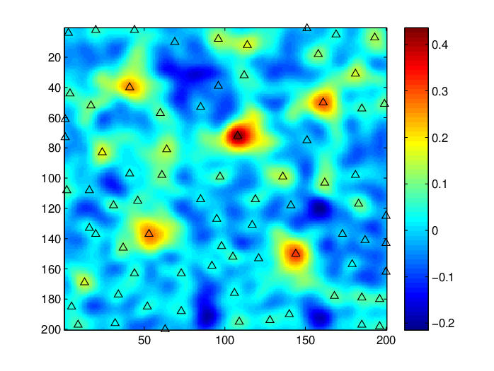
Figure 5 (top left) shows the first of those images, covering a region of about 10×10​μ​m210\times 10~\mu m^{2}. The background in this image has been log-transformed and adjusted by robust background estimates so that it can be assumed to have zero mean and unit variance. Pixelwise thresholding using the standard normal distribution for computing p-values and the BH algorithm on 85833 pixels per image times 1000 images at an FDR level of 0.0001 detects only the brightest regions (top middle) and provides a result where the FDR can only be interpreted in terms of pixels, not molecules.

The proper interpretation is given by the STEM algorithm. Considering the fluorescent molecules as point sources, the model of Section 2.1 captures the spatial extent of the signal peaks and the smoothness of the background field caused by dispersion of the recorded light in the acquisition process. The peak shape is seen in Figure 5 (top right), obtained as the average of the strongest peaks in the dataset, one from each image frame, aligned at their highest point. Robust estimation of the covariance function by rows and columns separately and across the image stack (not shown) indicates that the background noise may be modeled roughly by an isotropic Gaussian random field.

As shown in the simulation studies of Section 5, a rough approximation to the peak shape suffices to obtain good detection power. To smooth the images (bottom left), we use an isotropic Gaussian smoothing kernel fitted by least squares to the estimated peak shape in the log domain, yielding γ=1.6\gamma=1.6, and standardize the smoothed field so that the background has again mean zero and standard deviation σγ=1\sigma_{\gamma}=1. The choice of a Gaussian kernel allows using κγ=1\kappa_{\gamma}=1 in the height distribution of Section 3.4 for computing p-values, so that no correlation parameters need to be estimated. Thresholding the local maxima by the BH algorithm applied to the entire image stack at an FDR level of 0.0001 results in about 18 to 19 detected peaks in each frame (bottom middle).

Removing the isotropy assumption for the noise and computing p-values of the local maxima using the approximate overshoot distribution of Section 4 instead with pre-threshold v=1.8​σγv=1.8\sigma_{\gamma} (close to optimal according to Figure 4) yields the same significant peaks (bottom right). This confirms the simulation results that using the approximate overshoot distribution yields a similar power, while being more general in its required assumptions.

7 Technical details

7.1 Supporting results

Lemma 9.

Assume the model of Section 2.1 and let

E=sup‖x‖=1Var⁡(⟨∇zγ​(t),x⟩),F=sup‖x‖=1Var⁡(xT​∇2zγ​(t)​x).E=\sup_{\|x\|=1}{\rm Var}({\langle}\nabla z_{\gamma}(t),x\rangle),\quad F=\sup_{\|x\|=1}{\rm Var}(x^{T}\nabla^{2}z_{\gamma}(t)x).

For each jj, let uu and ε0>0\varepsilon_{0}>0 be fixed, then for sufficiently large aja_{j},

P(#{t∈T~∩Ijside}=0)≥1−exp⁡(−aj2​Cj22​E+ε0),P(#{t∈T~∩Ijmode}=1)≥1−exp⁡(−aj2​Cj22​E+ε0)−exp⁡(−aj2​Dj22​F+ε0),P(#{t∈T~(u)∩Ijmode}=1)≥1−Φ⁡(u−aj​Mjσγ)−exp⁡(−aj2​Dj22​F+ε0).\begin{split}{\rm P}\left(\#\{t\in\tilde{T}\cap I_{j}^{\rm side}\}=0\right)&\geq 1-\exp\left(-\frac{a_{j}^{2}C_{j}^{2}}{2E+\varepsilon_{0}}\right),\\ {\rm P}\left(\#\{t\in\tilde{T}\cap I_{j}^{\rm mode}\}=1\right)&\geq 1-\exp\left(-\frac{a_{j}^{2}C_{j}^{2}}{2E+\varepsilon_{0}}\right)-\exp\left(-\frac{a_{j}^{2}D_{j}^{2}}{2F+\varepsilon_{0}}\right),\\ {\rm P}\left(\#\{t\in\tilde{T}(u)\cap I_{j}^{\rm mode}\}=1\right)&\geq 1-\Phi\left(\frac{u-a_{j}M_{j}}{\sigma_{\gamma}}\right)-\exp\left(-\frac{a_{j}^{2}D_{j}^{2}}{2F+\varepsilon_{0}}\right).\end{split} (29)
Proof.

(1) Consider first the side region IjsideI_{j}^{\rm side}. The probability that there are no local maxima of yγ​(t)y_{\gamma}(t) in IjsideI_{j}^{\rm side} is greater than the probability that ⟨∇yγ​(t),τj−t⟩>0{\langle}\nabla y_{\gamma}(t),\tau_{j}-t\rangle>0 for all t∈Ijsidet\in I_{j}^{\rm side}. This probability is bounded below by

P(infIjside⟨∇zγ(t),τj−t⟩>−infIjside⟨∇μγ(t),τj−t⟩)=1−P(supIjside−⟨∇zγ(t),(τj−t)/∥τj−t∥⟩≥ajCj)≥1−P⁡(supt∈Ijsidesup‖x‖=1⟨∇zγ​(t),x⟩≥aj​Cj).\begin{split}{\rm P}&\left(\inf_{I_{j}^{\rm side}}{\langle}\nabla z_{\gamma}(t),\tau_{j}-t\rangle>-\inf_{I_{j}^{\rm side}}{\langle}\nabla\mu_{\gamma}(t),\tau_{j}-t\rangle\right)\\ &=1-{\rm P}\left(\sup_{I_{j}^{\rm side}}-{\langle}\nabla z_{\gamma}(t),(\tau_{j}-t)/\|\tau_{j}-t\|\rangle\geq a_{j}C_{j}\right)\\ &\geq 1-{\rm P}\left(\sup_{t\in I_{j}^{\rm side}}\sup_{\|x\|=1}{\langle}\nabla z_{\gamma}(t),x\rangle\geq a_{j}C_{j}\right).\end{split}

Then the first line of (29) follows from the Borell-TIS inequality [1, Eq. (4.1.1)] and the stationarity of zγz_{\gamma}.

(2) The probability that yγ​(t)y_{\gamma}(t) has no local maxima in IjmodeI_{j}^{\rm mode} is less than the probability that there exists some t∈∂Ijmodet\in\partial I_{j}^{\rm mode} such that ⟨∇yγ​(t),τj−t⟩≤0{\langle}\nabla y_{\gamma}(t),\tau_{j}-t\rangle\leq 0, for all t∈∂Ijmodet\in\partial I_{j}^{\rm mode} satisfying ⟨∇yγ​(t),τj−t⟩>0{\langle}\nabla y_{\gamma}(t),\tau_{j}-t\rangle>0 would imply the existence of at least one local maximum in IjI_{j}. This probability is bounded above by

P\displaystyle{\rm P} (inf∂Ijmode⟨∇zγ(t),τj−t⟩≤−inf∂Ijmode⟨∇μγ(t),τj−t⟩)\displaystyle\left(\inf_{\partial I_{j}^{\rm mode}}{\langle}\nabla z_{\gamma}(t),\tau_{j}-t\rangle\leq-\inf_{\partial I_{j}^{\rm mode}}{\langle}\nabla\mu_{\gamma}(t),\tau_{j}-t\rangle\right)
=P(sup∂Ijmode−⟨∇zγ(t),τj−t‖τj−t‖⟩≥inf∂Ijmode⟨∇μγ(t),τj−t‖τj−t‖⟩)\displaystyle={\rm P}\left(\sup_{\partial I_{j}^{\rm mode}}-\bigg\langle\nabla z_{\gamma}(t),\frac{\tau_{j}-t}{\|\tau_{j}-t\|}\bigg\rangle\geq\inf_{\partial I_{j}^{\rm mode}}\bigg\langle\nabla\mu_{\gamma}(t),\frac{\tau_{j}-t}{\|\tau_{j}-t\|}\bigg\rangle\right)
≤P⁡(supt∈Ijsidesup‖x‖=1⟨∇zγ​(t),x⟩≥aj​Cj),\displaystyle\leq{\rm P}\left(\sup_{t\in I_{j}^{\rm side}}\sup_{\|x\|=1}{\langle}\nabla z_{\gamma}(t),x\rangle\geq a_{j}C_{j}\right),

where the last inequality is due to fact that ∂Ijmode\partial I_{j}^{\rm mode} is contained in the closure of IjsideI_{j}^{\rm side}. Then by the Borell-TIS inequality, for any fixed ε0>0\varepsilon_{0}>0 and sufficiently large aja_{j},

P(#{t∈T~∩Ijmode)}=0)≤exp(−aj2​Cj22​E+ε0).{\rm P}\left(\#\{t\in\tilde{T}\cap I_{j}^{\rm mode})\}=0\right)\leq\exp\left(-\frac{a_{j}^{2}C_{j}^{2}}{2E+\varepsilon_{0}}\right). (30)

On the other hand, the probability that yγ​(t)y_{\gamma}(t) has more than one local maxima in IjmodeI_{j}^{\rm mode} is less than the probability that the largest eigenvalue of ∇2yγ​(t)\nabla^{2}y_{\gamma}(t) is nonnegative for some tt in IjmodeI_{j}^{\rm mode}. This probability is

P⁡(supt∈Ijmodesup‖x‖=1xT​∇2yγ​(t)​x≥0)≤P⁡(supt∈Ijmodesup‖x‖=1xT​∇2zγ​(t)​x≥aj​Dj).\displaystyle{\rm P}\left(\sup_{t\in I_{j}^{\rm mode}}\sup_{\|x\|=1}x^{T}\nabla^{2}y_{\gamma}(t)x\geq 0\right)\leq{\rm P}\left(\sup_{t\in I_{j}^{\rm mode}}\sup_{\|x\|=1}x^{T}\nabla^{2}z_{\gamma}(t)x\geq a_{j}D_{j}\right).

Then by the Borell-TIS inequality again, for any fixed ε0>0\varepsilon_{0}>0 and sufficiently large aja_{j},

P(#{t∈T~∩Ijmode)}≥2)≤exp(−aj2​Dj22​F+ε0).{\rm P}\left(\#\{t\in\tilde{T}\cap I_{j}^{\rm mode})\}\geq 2\right)\leq\exp\left(-\frac{a_{j}^{2}D_{j}^{2}}{2F+\varepsilon_{0}}\right). (31)

Putting (30) and (31) together gives the bound in the second line of (29).

(3) The probability that no local maxima of yγ​(t)y_{\gamma}(t) in IjmodeI_{j}^{\rm mode} exceed the threshold uu is less than the probability that yγ​(t)y_{\gamma}(t) is below uu anywhere in IjmodeI_{j}^{\rm mode}, so it is bounded above by Φ⁡[(u−aj​Mj)/σγ]\Phi[(u-a_{j}M_{j})/\sigma_{\gamma}]. On the other hand, the probability that more than one local maxima of yγ​(t)y_{\gamma}(t) in IjmodeI_{j}^{\rm mode} exceed uu is less than the probability that there exist more than one local maximum, which is bounded above by (31). Putting the two together gives the bound in the last line of (29). ∎

Remark 10.

Recall the uniformity assumptions in our model in Section 2.1, especially supj|Sj,γ|<∞\sup_{j}|S_{j,\gamma}|<\infty and infjMj>0\inf_{j}M_{j}>0. It can be seen from the proof of Lemma 9 that there exist a universal K>0K>0 such that (29) holds for all jj with aj>Ka_{j}>K.

Lemma 11.

Assume the model of Section 2.1 and let m~1,γ=#⁡{T~∩𝕊1,γ}\tilde{m}_{1,\gamma}=\#\{\tilde{T}\cap\mathbb{S}_{1,\gamma}\} and m~1,γ(u)=#{t∈T~(u)∩𝕊1,γ}\tilde{m}_{1,\gamma}(u)=\#\{t\in\tilde{T}(u)\cap\mathbb{S}_{1,\gamma}\}. Under conditions (C1) and (C2), there exists some ε1>0\varepsilon_{1}>0 such that as L→∞L\to\infty,

P(#{t∈T~∩𝕋γ}≥1)=o⁡(e−ε1​a2),P⁡(m~1,γ=J)=1−o⁡(e−ε1​a2),P​(m~1,γ​(u)=J)=1−o⁡(e−ε1​a2),\begin{split}{\rm P}\left(\#\{t\in\tilde{T}\cap\mathbb{T}_{\gamma}\}\geq 1\right)&=o(e^{-\varepsilon_{1}a^{2}}),\\ {\rm P}\left(\tilde{m}_{1,\gamma}=J\right)&=1-o(e^{-\varepsilon_{1}a^{2}}),\\ {\rm P}\left(\tilde{m}_{1,\gamma}(u)=J\right)&=1-o(e^{-\varepsilon_{1}a^{2}}),\end{split} (32)

where o⁡(e−ε1​a2)=o⁡(L−N)o(e^{-\varepsilon_{1}a^{2}})=o(L^{-N}) by condition (C2).

Proof.

(1) Write 𝕋γ=∪j=1JTj,γ\mathbb{T}_{\gamma}=\cup_{j=1}^{J}T_{j,\gamma}, where Tj,γ=Sj,γ∖SjT_{j,\gamma}=S_{j,\gamma}\setminus S_{j} is the transition region for peak jj. Note that Tj,γT_{j,\gamma} is a subset of IjsideI_{j}^{\rm side} since Ijmode⊂SjI_{j}^{\rm mode}\subset S_{j}. By (29) and condition (C2), for sufficiently large LL, the required probability P(#{t∈T~∩𝕋γ}≥1){\rm P}(\#\{t\in\tilde{T}\cap\mathbb{T}_{\gamma}\}\geq 1) is bounded above by

∑j=1Jexp⁡(−aj2​Cj22​E+ε0)≤LN​exp⁡(−a2​C22​E+ε0).\sum_{j=1}^{J}\exp\left(-\frac{a_{j}^{2}C_{j}^{2}}{2E+\varepsilon_{0}}\right)\leq L^{N}\exp\left(-\frac{a^{2}C^{2}}{2E+\varepsilon_{0}}\right).

Now the first line of (32) follows from the fact that for any δ>0\delta>0

LN​exp⁡(−δ​a2)=exp⁡{a2​(N​log⁡La2−δ)}→0.L^{N}\exp(-\delta a^{2})=\exp\left\{a^{2}\left(\frac{N\log L}{a^{2}}-\delta\right)\right\}\to 0.

(2) By (29) and condition (C2), for sufficiently large JJ, the required probability is bounded below by

P[∩j=1J(#{t∈T~∩Ijmode}=1∩#{t∈T~∩Ijside}=0)]\displaystyle\rm{\displaystyle P}\left[\cap_{j=1}^{J}\left(\#\{t\in\tilde{T}\cap I_{j}^{\rm mode}\}=1~\cap~\#\{t\in\tilde{T}\cap I_{j}^{\rm side}\}=0\right)\right]
≥1−∑j=1J[1−P(#{t∈T~∩Ijmode}=1∩#{t∈T~∩Ijside}=0)]\displaystyle\geq 1-\sum_{j=1}^{J}\left[1-{\rm P}\left(\#\{t\in\tilde{T}\cap I_{j}^{\rm mode}\}=1~\cap~\#\{t\in\tilde{T}\cap I_{j}^{\rm side}\}=0\right)\right]
≥1−∑j=1J[2​exp⁡(−aj2​Cj22​E+ε0)+exp⁡(−aj2​Dj22​F+ε0)]\displaystyle\geq 1-\sum_{j=1}^{J}\left[2\exp\left(-\frac{a_{j}^{2}C_{j}^{2}}{2E+\varepsilon_{0}}\right)+\exp\left(-\frac{a_{j}^{2}D_{j}^{2}}{2F+\varepsilon_{0}}\right)\right]
≥1−2​LN​exp⁡(−a2​C22​E+ε0)−LN​exp⁡(−a2​D22​F+ε0),\displaystyle\geq 1-2L^{N}\exp\left(-\frac{a^{2}C^{2}}{2E+\varepsilon_{0}}\right)-L^{N}\exp\left(-\frac{a^{2}D^{2}}{2F+\varepsilon_{0}}\right),

where D>0D>0 is the infimum of the DiD_{i}’s. The second line of (32) follows.

(3) Applying the last line of (29), together with similar argument in step (2), yields the last line of (32). ∎

Lemma 12.

Assume the model of Section 2.1 and let m~​(v)\tilde{m}(v) be as defined in Section 2.2. Then Var⁡(m~​(v))=O⁡(LN){\rm Var}(\tilde{m}(v))=O(L^{N}) as L→∞L\to\infty.

Proof.

By the Kac-Rice formula [1], E​[m~​(v)]{\rm E}[\tilde{m}(v)] equals

∫U⁡(L)E⁡{|det​∇2yγ​(t)|​𝟙{yγ​(t)>v,∇2yγ​(t)≺0}|∇yγ​(t)=0}​p∇yγ​(t)​(0)​𝑑t\int_{U(L)}{\rm E}\{|{\rm det}\nabla^{2}y_{\gamma}(t)|\mathbbm{1}_{\{y_{\gamma}(t)>v,\nabla^{2}y_{\gamma}(t)\prec 0\}}|\nabla y_{\gamma}(t)=0\}p_{\nabla y_{\gamma}(t)}(0)dt

and E​[m~​(v)​(m~​(v)−1)]{\rm E}[\tilde{m}(v)(\tilde{m}(v)-1)] equals

∫U⁡(L)∫U⁡(L)E{|det∇2yγ(t)||det∇2yγ(s)|𝟙{yγ​(t)>v,∇2yγ​(t)≺0}×𝟙{yγ​(s)>v,∇2yγ​(s)≺0}|∇yγ(t)=0,∇yγ(s)=0}p∇yγ​(t),∇yγ​(s)(0,0)dtds.\begin{split}&\int_{U(L)}\int_{U(L)}{\rm E}\{|{\rm det}\nabla^{2}y_{\gamma}(t)||{\rm det}\nabla^{2}y_{\gamma}(s)|\mathbbm{1}_{\{y_{\gamma}(t)>v,\nabla^{2}y_{\gamma}(t)\prec 0\}}\\ &\quad\times\mathbbm{1}_{\{y_{\gamma}(s)>v,\nabla^{2}y_{\gamma}(s)\prec 0\}}|\nabla y_{\gamma}(t)=0,\nabla y_{\gamma}(s)=0\}p_{\nabla y_{\gamma}(t),\nabla y_{\gamma}(s)}(0,0)dtds.\end{split}

It then follows from the observation Var⁡(m~)=E⁡[m~​(m~−1)]+E⁡[m~]−(E⁡[m~])2{\rm Var}(\tilde{m})={\rm E}[\tilde{m}(\tilde{m}-1)]+{\rm E}[\tilde{m}]-({\rm E}[\tilde{m}])^{2} that Var⁡(m~){\rm Var}(\tilde{m}) can be written as

∫U⁡(L)∫U⁡(L)(E{|det∇2yγ(t)||det∇2yγ(s)|𝟙{yγ​(t)>v,∇2yγ​(t)≺0}×𝟙{yγ​(s)>v,∇2yγ​(s)≺0}|∇yγ(t)=0,∇yγ(s)=0}p∇yγ​(t),∇yγ​(s)(0,0)−E⁡{|det​∇2yγ​(t)|​𝟙{yγ​(t)>v,∇2yγ​(t)≺0}|∇yγ​(t)=0}​p∇yγ​(t)​(0)×E{|det∇2yγ(s)|𝟙{yγ​(s)>v,∇2yγ​(s)≺0}|∇yγ(s)=0}p∇yγ​(s)(0))dtds+∫U⁡(L)E{|det∇2yγ(t)|𝟙{yγ​(t)>v,∇2yγ​(t)≺0}|∇yγ(t)=0}p∇yγ​(t)(0)dt:=∫U⁡(L)∫U⁡(L)f1​(t,s)​dt​ds+∫U⁡(L)f2​(t)​dt:=I1+I2.\begin{split}&\int_{U(L)}\int_{U(L)}\Big({\rm E}\{|{\rm det}\nabla^{2}y_{\gamma}(t)||{\rm det}\nabla^{2}y_{\gamma}(s)|\mathbbm{1}_{\{y_{\gamma}(t)>v,\nabla^{2}y_{\gamma}(t)\prec 0\}}\\ &\quad\times\mathbbm{1}_{\{y_{\gamma}(s)>v,\nabla^{2}y_{\gamma}(s)\prec 0\}}|\nabla y_{\gamma}(t)=0,\nabla y_{\gamma}(s)=0\}p_{\nabla y_{\gamma}(t),\nabla y_{\gamma}(s)}(0,0)\\ &\quad-{\rm E}\{|{\rm det}\nabla^{2}y_{\gamma}(t)|\mathbbm{1}_{\{y_{\gamma}(t)>v,\nabla^{2}y_{\gamma}(t)\prec 0\}}|\nabla y_{\gamma}(t)=0\}p_{\nabla y_{\gamma}(t)}(0)\\ &\quad\times{\rm E}\{|{\rm det}\nabla^{2}y_{\gamma}(s)|\mathbbm{1}_{\{y_{\gamma}(s)>v,\nabla^{2}y_{\gamma}(s)\prec 0\}}|\nabla y_{\gamma}(s)=0\}p_{\nabla y_{\gamma}(s)}(0)\Big)dtds\\ &\quad+\int_{U(L)}{\rm E}\{|{\rm det}\nabla^{2}y_{\gamma}(t)|\mathbbm{1}_{\{y_{\gamma}(t)>v,\nabla^{2}y_{\gamma}(t)\prec 0\}}|\nabla y_{\gamma}(t)=0\}p_{\nabla y_{\gamma}(t)}(0)dt\\ &:=\int_{U(L)}\int_{U(L)}f_{1}(t,s)dtds+\int_{U(L)}f_{2}(t)dt:=I_{1}+I_{2}.\end{split}

Recall yγ​(t)=zγ​(t)+μγ​(t)y_{\gamma}(t)=z_{\gamma}(t)+\mu_{\gamma}(t), where μγ​(t)=∑j=−∞∞aj​hj,γ​(t)\mu_{\gamma}(t)=\sum_{j=-\infty}^{\infty}a_{j}h_{j,\gamma}(t) and zγ​(t)z_{\gamma}(t) is stationary. Assume t∈Sj,γt\in S_{j,\gamma} for some jj, then

f2​(t)≤E{|det(∇2zγ(0)+aj∇2hj,γ(t))||∇zγ(0)+aj∇hj,γ(t)=0}×exp[−aj2[∇hj,γ(t)]T[Cov(∇zγ(0))]−1∇hj,γ(t)/2](2​π)N/2​[detCov⁡(∇zγ​(0))]1/2≤c1​(ajn1+1)​exp⁡[−c2​aj2]≤c3\begin{split}f_{2}(t)&\leq{\rm E}\{|{\rm det}(\nabla^{2}z_{\gamma}(0)+a_{j}\nabla^{2}h_{j,\gamma}(t))||\nabla z_{\gamma}(0)+a_{j}\nabla h_{j,\gamma}(t)=0\}\\ &\quad\times\frac{\exp\left[-a_{j}^{2}[\nabla h_{j,\gamma}(t)]^{T}[{\rm Cov}(\nabla z_{\gamma}(0))]^{-1}\nabla h_{j,\gamma}(t)/2\right]}{(2\pi)^{N/2}[{\rm detCov}(\nabla z_{\gamma}(0))]^{1/2}}\\ &\leq c_{1}(a_{j}^{n_{1}}+1)\exp[-c_{2}a_{j}^{2}]\leq c_{3}\end{split} (33)

for some positive constants n1n_{1}, c1c_{1}, c2c_{2} and c3c_{3}. Similar result holds for tt such that μγ​(t)=0\mu_{\gamma}(t)=0. Therefore I2=O⁡(LN)I_{2}=O(L^{N}).

We consider a pair of independent Gaussian fields z~γ​(t)\tilde{z}_{\gamma}(t) and z~γ​(s)\tilde{z}_{\gamma}(s) with the distribution of zγ​(t)z_{\gamma}(t) and zγ​(s)z_{\gamma}(s) respectively, assume also that z~γ​(t)\tilde{z}_{\gamma}(t) and z~γ​(s)\tilde{z}_{\gamma}(s) are both independent of zγ​(t)z_{\gamma}(t) and zγ​(s)z_{\gamma}(s). Let

Z1​(t,s)=(zγ(t),zγ(s)),Y1(t,s)=Z1(t,s)+(μγ(t),μγ(s)),Z0​(t,s)=(z~γ(t),z~γ(s)),Y0(t,s)=Z0(t,s)+(μγ(t),μγ(s)),\begin{split}Z_{1}(t,s)&=(z_{\gamma}(t),z_{\gamma}(s)),\quad Y_{1}(t,s)=Z_{1}(t,s)+(\mu_{\gamma}(t),\mu_{\gamma}(s)),\\ Z_{0}(t,s)&=(\tilde{z}_{\gamma}(t),\tilde{z}_{\gamma}(s)),\quad Y_{0}(t,s)=Z_{0}(t,s)+(\mu_{\gamma}(t),\mu_{\gamma}(s)),\\ \end{split}

and let F⁡(x,y,A,B)=|det⁡(A)|​|det⁡(B)|​𝟙{x>v,A≺0}​𝟙{y>v,B≺0}F(x,y,A,B)=|{\rm det}(A)||{\rm det}(B)|\mathbbm{1}_{\{x>v,A\prec 0\}}\mathbbm{1}_{\{y>v,B\prec 0\}}, where x,y∈ℝx,y\in\mathbb{R} and AA and BB are N×NN\times N symmetric matrices. Then

f1​(t,s)=E⁡{F⁡(Y1​(t,s),∇2Y1​(t,s))|∇Y1​(t,s)=0}​p∇Y1​(t,s)​(0)−E⁡{F⁡(Y0​(t,s),∇2Y0​(t,s))|∇Y0​(t,s)=0}​p∇Y0​(t,s)​(0).\begin{split}f_{1}(t,s)&={\rm E}\{F(Y_{1}(t,s),\nabla^{2}Y_{1}(t,s))|\nabla Y_{1}(t,s)=0\}p_{\nabla Y_{1}(t,s)}(0)\\ &\quad-{\rm E}\{F(Y_{0}(t,s),\nabla^{2}Y_{0}(t,s))|\nabla Y_{0}(t,s)=0\}p_{\nabla Y_{0}(t,s)}(0).\end{split}

Let

Yη​(t,s)=η​Z1​(t,s)+1−η​Z0​(t,s)+(μγ​(t),μγ​(s)),Yη′​(t,s)=η∇Z1(t,s)+1−η∇Z0(t,s)+(∇μγ(t),∇μγ(s)),Yη′′(t,s)=η​∇2Z1​(t,s)+1−η​∇2Z0​(t,s)+(∇2μγ​(t),∇2μγ​(s)),\begin{split}Y_{\eta}(t,s)&=\sqrt{\eta}Z_{1}(t,s)+\sqrt{1-\eta}Z_{0}(t,s)+(\mu_{\gamma}(t),\mu_{\gamma}(s)),\\ Y_{\eta}^{\prime}(t,s)&=\sqrt{\eta}\nabla Z_{1}(t,s)+\sqrt{1-\eta}\nabla Z_{0}(t,s)+(\nabla\mu_{\gamma}(t),\nabla\mu_{\gamma}(s)),\\ Y_{\eta}^{{}^{\prime\prime}}(t,s)&=\sqrt{\eta}\nabla^{2}Z_{1}(t,s)+\sqrt{1-\eta}\nabla^{2}Z_{0}(t,s)+(\nabla^{2}\mu_{\gamma}(t),\nabla^{2}\mu_{\gamma}(s)),\end{split}

and denote by Rη​(i,j)R_{\eta}(i,j) the (i,j)(i,j) entry of Cov(Yη(t,s),Yη′(t,s),Yη′′(t,s)){\rm Cov}(Y_{\eta}(t,s),Y_{\eta}^{\prime}(t,s),Y_{\eta}^{{}^{\prime\prime}}(t,s)). It follows that f1​(t,s)f_{1}(t,s) can be written as

∫01dd​η(E{F(Yη(t,s),Yη′′(t,s))|Yη′(t,s)=0}pYη′​(t,s)(0))dη=∫01dd​η∫ℝ2+N⁡(N+1)F(ξ)p(Yη(t,s),Yη′′(t,s)),Yη′(t,s)(ξ,0)dξdη=∫01∫ℝ2+N⁡(N+1)F(ξ)dd​ηp(Yη(t,s),Yη′′(t,s)),Yη′(t,s)(ξ,0)dξdη=∫01∫ℝ2+N⁡(N+1)F⁡(ξ)​(∑i,j∂p(Yη(t,s),Yη′′(t,s)),Yη′(t,s)(ξ,0)∂Rη​(i,j)​∂Rη​(i,j)∂η)​dξ​dη.\begin{split}&\quad\int_{0}^{1}\frac{d}{d\eta}\left({\rm E}\{F(Y_{\eta}(t,s),Y_{\eta}^{{}^{\prime\prime}}(t,s))|Y_{\eta}^{\prime}(t,s)=0\}p_{Y_{\eta}^{\prime}(t,s)}(0)\right)d\eta\\ &=\int_{0}^{1}\frac{d}{d\eta}\int_{\mathbb{R}^{2+N(N+1)}}F(\xi)p_{(Y_{\eta}(t,s),Y_{\eta}^{{}^{\prime\prime}}(t,s)),Y_{\eta}^{\prime}(t,s)}(\xi,0)d\xi d\eta\\ &=\int_{0}^{1}\int_{\mathbb{R}^{2+N(N+1)}}F(\xi)\frac{d}{d\eta}p_{(Y_{\eta}(t,s),Y_{\eta}^{{}^{\prime\prime}}(t,s)),Y_{\eta}^{\prime}(t,s)}(\xi,0)d\xi d\eta\\ &=\int_{0}^{1}\int_{\mathbb{R}^{2+N(N+1)}}F(\xi)\left(\sum_{i,j}\frac{\partial p_{(Y_{\eta}(t,s),Y_{\eta}^{{}^{\prime\prime}}(t,s)),Y_{\eta}^{\prime}(t,s)}(\xi,0)}{\partial R_{\eta}(i,j)}\frac{\partial R_{\eta}(i,j)}{\partial\eta}\right)d\xi d\eta.\end{split}

By a well-known formula for Gaussian density which is similar to the heat equation [1, Eq. (2.2.6)] and the fact that Rη​(i,j)=η​R1​(i,j)+(1−η)​R0​(i,j)R_{\eta}(i,j)=\eta R_{1}(i,j)+(1-\eta)R_{0}(i,j), we see that

|f1​(t,s)|≤∑i,j|∫01∫ℝ2+N⁡(N+1)F⁡(ξ)​∂2p(Yη(t,s),Yη′′(t,s)),Yη′(t,s)(y)∂yi​∂yj|y=(ξ,0)​dξ​dη|×|R1​(i,j)−R0​(i,j)|.\begin{split}|f_{1}(t,s)|&\leq\sum_{i,j}\left|\int_{0}^{1}\int_{\mathbb{R}^{2+N(N+1)}}F(\xi)\frac{\partial^{2}p_{(Y_{\eta}(t,s),Y_{\eta}^{{}^{\prime\prime}}(t,s)),Y_{\eta}^{\prime}(t,s)}(y)}{\partial y_{i}\partial y_{j}}\Big|_{y=(\xi,0)}d\xi d\eta\right|\\ &\qquad\quad\times|R_{1}(i,j)-R_{0}(i,j)|.\end{split}

Similarly to (33), there exists a positive constant c4c_{4} such that

|∫01∫ℝ2+N⁡(N+1)F⁡(ξ)​∂2p(Yη(t,s),Yη′′(t,s)),Yη′(t,s)(y)∂yi​∂yj|y=(ξ,0)​dξ​dη|≤c4\begin{split}\left|\int_{0}^{1}\int_{\mathbb{R}^{2+N(N+1)}}F(\xi)\frac{\partial^{2}p_{(Y_{\eta}(t,s),Y_{\eta}^{{}^{\prime\prime}}(t,s)),Y_{\eta}^{\prime}(t,s)}(y)}{\partial y_{i}\partial y_{j}}\Big|_{y=(\xi,0)}d\xi d\eta\right|\leq c_{4}\end{split}

for all ii and jj.

Recall rγ​(t)=E⁡[zγ​(t)​zγ​(0)]r_{\gamma}(t)={\rm E}[z_{\gamma}(t)z_{\gamma}(0)] in Section 2.1. By stationarity and change of variables, we obtain

|I1|≤8c42NLN∑i,j,k,l=1N∫0L⋯∫0L(∏i=1N(1−tiL))(|rγ(t)|+|∂rγ​(t)∂ti|+|∂2rγ​(t)∂ti​∂tj|+|∂3rγ​(t)∂ti​∂tj​∂tk|+|∂4rγ​(t)∂ti​∂tj​∂tk​∂tl|)dt1⋯dtN.\begin{split}|I_{1}|&\leq 8c_{4}2^{N}L^{N}\sum_{i,j,k,l=1}^{N}\int_{0}^{L}\cdots\int_{0}^{L}\left(\prod_{i=1}^{N}\bigg(1-\frac{t_{i}}{L}\bigg)\right)\Bigg(|r_{\gamma}(t)|+\left|\frac{\partial r_{\gamma}(t)}{\partial t_{i}}\right|\\ &\quad+\left|\frac{\partial^{2}r_{\gamma}(t)}{\partial t_{i}\partial t_{j}}\right|+\left|\frac{\partial^{3}r_{\gamma}(t)}{\partial t_{i}\partial t_{j}\partial t_{k}}\right|+\left|\frac{\partial^{4}r_{\gamma}(t)}{\partial t_{i}\partial t_{j}\partial t_{k}\partial t_{l}}\right|\Bigg)dt_{1}\cdots dt_{N}.\end{split}

Condition (5) implies that the last integral above is finite as L→∞L\to\infty, hence I1=O⁡(LN)I_{1}=O(L^{N}), completing the proof. ∎

Lemma 13.

Assume the model of Section 2.1 and let m~1,γ\tilde{m}_{1,\gamma} and m~1,γ​(u)\tilde{m}_{1,\gamma}(u) be as defined in Lemma 11. Then

E⁡[m~1,γ]/J=1+O⁡(a−2),E⁡[m~1,γ​(u)]/J=1+O⁡(a−2).{\rm E}[\tilde{m}_{1,\gamma}]/J=1+O(a^{-2}),\quad{\rm E}[\tilde{m}_{1,\gamma}(u)]/J=1+O(a^{-2}).
Proof.

We only prove the first part since the second part can be derived similarly. By the Kac-Rice formula [1], E⁡[m~1,γ]=∑j=1JI⁡(Sj,γ){\rm E}[\tilde{m}_{1,\gamma}]=\sum_{j=1}^{J}I(S_{j,\gamma}), where

I⁡(Sj,γ)=∫Sj,γE{|det∇2yγ(t)|𝟙{∇2yγ(t)≺0}|∇yγ(t)=0}p∇yγ​(t)(0)dt=1(2​π)N/2​det⁡(Λγ)∫Sj,γE{|det(∇2zγ(0)+aj∇2hj,γ(t))|×𝟙{∇2zγ(0)+aj∇2hj,γ(t)≺0}|∇zγ(0)+aj∇hj,γ(t)=0}×exp{−aj2[∇hj,γ(t)]TΛγ−1∇hj,γ(t)/2}dt.\begin{split}I(S_{j,\gamma})&=\int_{S_{j,\gamma}}{\rm E}\left\{|{\rm det}\nabla^{2}y_{\gamma}(t)|\mathbbm{1}_{\{\nabla^{2}y_{\gamma}(t)\prec 0\}}\big|\nabla y_{\gamma}(t)=0\right\}p_{\nabla y_{\gamma}(t)}(0)dt\\ &=\frac{1}{(2\pi)^{N/2}\sqrt{{\rm det}(\Lambda_{\gamma})}}\int_{S_{j,\gamma}}{\rm E}\big\{|{\rm det}(\nabla^{2}z_{\gamma}(0)+a_{j}\nabla^{2}h_{j,\gamma}(t))|\\ &\quad\times\mathbbm{1}_{\{\nabla^{2}z_{\gamma}(0)+a_{j}\nabla^{2}h_{j,\gamma}(t)\prec 0\}}\big|\nabla z_{\gamma}(0)+a_{j}\nabla h_{j,\gamma}(t)=0\big\}\\ &\quad\times\exp\left\{-a_{j}^{2}[\nabla h_{j,\gamma}(t)]^{T}\Lambda_{\gamma}^{-1}\nabla h_{j,\gamma}(t)/2\right\}dt.\end{split}

Let f(t)=[∇hj,γ(t)]TΛγ−1∇hj,γ(t)/2f(t)=[\nabla h_{j,\gamma}(t)]^{T}\Lambda_{\gamma}^{-1}\nabla h_{j,\gamma}(t)/2, which attains the minimum 0 only at τj\tau_{j} over Sj,γS_{j,\gamma} such that

∇2f​(τj)=∇2hj,γ​(τj)​Λγ−1​∇2hj,γ​(τj).\nabla^{2}f(\tau_{j})=\nabla^{2}h_{j,\gamma}(\tau_{j})\Lambda_{\gamma}^{-1}\nabla^{2}h_{j,\gamma}(\tau_{j}). (34)

Let IjmodeI_{j}^{\rm mode}, CC and DD be as defined in Section 2.1. Since C>0C>0, f⁡(t)f(t) is strictly greater than 0 over Sj,γ\IjmodeS_{j,\gamma}\backslash I_{j}^{\rm mode} , and there exists some ε0>0\varepsilon_{0}>0 such that I⁡(Sj,γ)=I⁡(Ijmode)+o⁡(e−ε0​a2)I(S_{j,\gamma})=I(I_{j}^{\rm mode})+o(e^{-\varepsilon_{0}a^{2}}) for all jj. Moreover, since D>0D>0, a similar argument as in the proof of [6, Theorem 2.4] yields that removing the indicator function 𝟙{∇2zγ(0)+aj∇2hj,γ(t)≺0}\mathbbm{1}_{\{\nabla^{2}z_{\gamma}(0)+a_{j}\nabla^{2}h_{j,\gamma}(t)\prec 0\}} in the expression of I⁡(Ijmode)I(I_{j}^{\rm mode}) only causes an error of rate o⁡(e−ε1​a2)o(e^{-\varepsilon_{1}a^{2}}), where ε1>0\varepsilon_{1}>0 is some constant. Now, applying the Laplace method to the expression

1(2​π)N/2​det⁡(Λγ)∫IjmodeE{|det(∇2zγ(0)+aj∇2hj,γ(t))|×𝟙{∇2zγ(0)+aj∇2hj,γ(t)≺0}|∇zγ(0)+aj∇hj,γ(t)=0}exp{−aj2f(t)}dt,\begin{split}&\frac{1}{(2\pi)^{N/2}\sqrt{{\rm det}(\Lambda_{\gamma})}}\int_{I_{j}^{\rm mode}}{\rm E}\big\{|{\rm det}(\nabla^{2}z_{\gamma}(0)+a_{j}\nabla^{2}h_{j,\gamma}(t))|\\ &\quad\times\mathbbm{1}_{\{\nabla^{2}z_{\gamma}(0)+a_{j}\nabla^{2}h_{j,\gamma}(t)\prec 0\}}\big|\nabla z_{\gamma}(0)+a_{j}\nabla h_{j,\gamma}(t)=0\big\}\exp\left\{-a_{j}^{2}f(t)\right\}dt,\end{split}

we obtain

I⁡(Sj,γ)=det⁡(aj​∇2hj,γ​(τj))(2​π)N/2​det⁡(Λγ)​((2​π)Naj2​N​det​(∇2f​(τj)))1/2+O⁡(aj−2)=1+O⁡(aj−2),\begin{split}I(S_{j,\gamma})&=\frac{{\rm det}(a_{j}\nabla^{2}h_{j,\gamma}(\tau_{j}))}{(2\pi)^{N/2}\sqrt{{\rm det}(\Lambda_{\gamma})}}\left(\frac{(2\pi)^{N}}{a_{j}^{2N}{\rm det}(\nabla^{2}f(\tau_{j}))}\right)^{1/2}+O(a_{j}^{-2})\\ &=1+O(a_{j}^{-2}),\end{split}

where the last line is due to (34). Therefore E⁡[m~1,γ]/J=1+O⁡(a−2){\rm E}[\tilde{m}_{1,\gamma}]/J=1+O(a^{-2}). ∎

7.2 Control of FDR

Proof of Theorem 3.

We prove part (ii) first, since part (i) is much easier and can be seen from the proof of part (ii). Let G~(u,v)=#{t∈T~(u)}/#{t∈T~(v)}\tilde{G}(u,v)=\#\{t\in\tilde{T}(u)\}/\#\{t\in\tilde{T}(v)\} be the empirical marginal right cdf of yγ​(t)y_{\gamma}(t) given t∈T~​(v)t\in\tilde{T}(v), where u>vu>v. Then the random BH threshold u~BH​(v)\tilde{u}_{{\rm BH}}(v) (14) satisfies

α​G~​(u~BH​(v),v)=k​α/m~​(v)=Fγ​(u~BH​(v),v),\alpha\tilde{G}(\tilde{u}_{{\rm BH}}(v),v)=k\alpha/\tilde{m}(v)=F_{\gamma}(\tilde{u}_{{\rm BH}}(v),v),

so u~BH​(v)\tilde{u}_{{\rm BH}}(v) is the smallest uu that is greater than vv and satisfies

α​G~​(u,v)≥Fγ​(u,v).\alpha\tilde{G}(u,v)\geq F_{\gamma}(u,v). (35)

The strategy is to solve equation (35) in the limit when L,a→∞L,a\to\infty. We first find the limit of G~​(u,v)\tilde{G}(u,v). Letting m~0,γ(u)=#{t∈T~(u)∩𝕊0,γ}\tilde{m}_{0,\gamma}(u)=\#\{t\in\tilde{T}(u)\cap\mathbb{S}_{0,\gamma}\} and m~1,γ(u)=#{t∈T~(u)∩𝕊1,γ}\tilde{m}_{1,\gamma}(u)=\#\{t\in\tilde{T}(u)\cap\mathbb{S}_{1,\gamma}\}, so that m~​(u)=m~0,γ​(u)+m~1,γ​(u)\tilde{m}(u)=\tilde{m}_{0,\gamma}(u)+\tilde{m}_{1,\gamma}(u), write

G~​(u,v)=m~​(u)m~​(v)=m~0,γ​(u)m~0,γ​(v)+m~1,γ​(v)+m~1,γ​(u)m~0,γ​(v)+m~1,γ​(v).\tilde{G}(u,v)=\frac{\tilde{m}(u)}{\tilde{m}(v)}=\frac{\tilde{m}_{0,\gamma}(u)}{\tilde{m}_{0,\gamma}(v)+\tilde{m}_{1,\gamma}(v)}+\frac{\tilde{m}_{1,\gamma}(u)}{\tilde{m}_{0,\gamma}(v)+\tilde{m}_{1,\gamma}(v)}. (36)

By Chebyshev’s inequality, Lemma 12 and condition (C2),

m~0,γ​(v)/LN=E[m~0,γ(v)]/LN+Op(L−N/2)=E[m~0,γ(U(1),v)](1−A2,γ)+Op(a−2+L−N/2).\begin{split}\tilde{m}_{0,\gamma}(v)/L^{N}&={\rm E}[\tilde{m}_{0,\gamma}(v)]/L^{N}+O_{p}(L^{-N/2})\\ &={\rm E}[\tilde{m}_{0,\gamma}(U(1),v)](1-A_{2,\gamma})+O_{p}(a^{-2}+L^{-N/2}).\end{split}

On the other hand, by Lemma 13 and condition (C2),

m~1,γ(v)/LN=E[m~1,γ(v)]/LN+Op(L−N/2)=A1+Op(a−2+L−N/2).\begin{split}\tilde{m}_{1,\gamma}(v)/L^{N}={\rm E}[\tilde{m}_{1,\gamma}(v)]/L^{N}+O_{p}(L^{-N/2})=A_{1}+O_{p}(a^{-2}+L^{-N/2}).\end{split}

Therefore, (36) can be written as

G~​(u,v)=E⁡[m~0,γ​(U⁡(1),u)]​(1−A2,γ)+A1E⁡[m~0,γ​(U⁡(1),v)]​(1−A2,γ)+A1+Op(a−2+L−N/2)=Fγ​(u,v)​E​[m~0,γ​(U⁡(1),v)]​(1−A2,γ)+A1E⁡[m~0,γ​(U⁡(1),v)]​(1−A2,γ)+A1+Op(a−2+L−N/2).\begin{split}\tilde{G}(u,v)&=\frac{{\rm E}[\tilde{m}_{0,\gamma}(U(1),u)](1-A_{2,\gamma})+A_{1}}{{\rm E}[\tilde{m}_{0,\gamma}(U(1),v)](1-A_{2,\gamma})+A_{1}}+O_{p}(a^{-2}+L^{-N/2})\\ &=\frac{F_{\gamma}(u,v){\rm E}[\tilde{m}_{0,\gamma}(U(1),v)](1-A_{2,\gamma})+A_{1}}{{\rm E}[\tilde{m}_{0,\gamma}(U(1),v)](1-A_{2,\gamma})+A_{1}}+O_{p}(a^{-2}+L^{-N/2}).\end{split}

Now replacing G~​(u,v)\tilde{G}(u,v) by its limit in (35), and solving for uu gives the deterministic solution

uBH∗​(v)=Fγ​(⋅,v)−1​(α​A1A1+E⁡[m~0,γ​(U⁡(1),v)]​(1−A2,γ)​(1−α)).u^{*}_{{\rm BH}}(v)=F_{\gamma}(\cdot,v)^{-1}\left(\frac{\alpha A_{1}}{A_{1}+{\rm E}[\tilde{m}_{0,\gamma}(U(1),v)](1-A_{2,\gamma})(1-\alpha)}\right). (37)

The argument above implies F(u~BH(v),v)=F(uBH∗(v),v)+Op(a−2+L−N/2)F(\tilde{u}_{{\rm BH}}(v),v)=F(u^{*}_{{\rm BH}}(v),v)+O_{p}(a^{-2}+L^{-N/2}), but the first-derivative of Fγ​(⋅,v)F_{\gamma}(\cdot,v) is uniformly bounded, thus u~BH(v)=uBH∗(v)+Op(a−2+L−N/2)\tilde{u}_{{\rm BH}}(v)=u^{*}_{{\rm BH}}(v)+O_{p}(a^{-2}+L^{-N/2}). Following similar arguments, together with Chebyshev’s inequality, we also have

P(|u~BH(v)−u∗BH(v)|>a−1+L−N/4)=O(a−1+L−N/4).\begin{split}{\rm P}\left(|\tilde{u}_{{\rm BH}}(v)-u^{*}_{{\rm BH}}(v)|>a^{-1}+L^{-N/4}\right)=O(a^{-1}+L^{-N/4}).\end{split} (38)

Next, let us turn to estimating E⁡[m~0,γ​(u~BH​(v))]{\rm E}[\tilde{m}_{0,\gamma}(\tilde{u}_{{\rm BH}}(v))]. Notice that,

|E⁡[(m~0,γ​(u~BH​(v))−m~0,γ​(uBH∗​(v)))/LN]|≤|E[(m~0,γ(u~BH(v))−m~0,γ(u∗BH(v)))/LN𝟙{|u~BH(v)−u∗BH(v)|≤a−1+L−N/4}]|+|E[(m~0,γ(u~BH(v))−m~0,γ(u∗BH(v)))/LN𝟙{|u~BH(v)−u∗BH(v)|>a−1+L−N/4}]|≤|E[(m~0,γ(u∗BH(v)−a−1−L−N/4)−m~0,γ(u∗BH(v)))/LN]|+|E[(m~0,γ(u∗BH(v))−m~0,γ(u∗BH(v)+a−1+L−N/4))/LN]|+2(E[m~(v)2]/L2​N)1/2P(|u~BH(v)−u∗BH(v)|>a−1+L−N/4)=O(a−1+L−N/4),\begin{split}&\quad\left|{\rm E}\left[(\tilde{m}_{0,\gamma}(\tilde{u}_{{\rm BH}}(v))-\tilde{m}_{0,\gamma}(u^{*}_{{\rm BH}}(v)))/L^{N}\right]\right|\\ &\leq\left|{\rm E}\left[(\tilde{m}_{0,\gamma}(\tilde{u}_{{\rm BH}}(v))-\tilde{m}_{0,\gamma}(u^{*}_{{\rm BH}}(v)))/L^{N}\mathbbm{1}_{\{|\tilde{u}_{{\rm BH}}(v)-u^{*}_{{\rm BH}}(v)|\leq a^{-1}+L^{-N/4}\}}\right]\right|\\ &\quad+\left|{\rm E}\left[(\tilde{m}_{0,\gamma}(\tilde{u}_{{\rm BH}}(v))-\tilde{m}_{0,\gamma}(u^{*}_{{\rm BH}}(v)))/L^{N}\mathbbm{1}_{\{|\tilde{u}_{{\rm BH}}(v)-u^{*}_{{\rm BH}}(v)|>a^{-1}+L^{-N/4}\}}\right]\right|\\ &\leq\left|{\rm E}\left[\left(\tilde{m}_{0,\gamma}\left(u^{*}_{{\rm BH}}(v)-a^{-1}-L^{-N/4}\right)-\tilde{m}_{0,\gamma}(u^{*}_{{\rm BH}}(v))\right)/L^{N}\right]\right|\\ &\quad+\left|{\rm E}\left[\left(\tilde{m}_{0,\gamma}(u^{*}_{{\rm BH}}(v))-\tilde{m}_{0,\gamma}\left(u^{*}_{{\rm BH}}(v)+a^{-1}+L^{-N/4}\right)\right)/L^{N}\right]\right|\\ &\quad+2\left({\rm E}\left[\tilde{m}(v)^{2}\right]/L^{2N}\right)^{1/2}{\rm P}\left(|\tilde{u}_{{\rm BH}}(v)-u^{*}_{{\rm BH}}(v)|>a^{-1}+L^{-N/4}\right)\\ &=O(a^{-1}+L^{-N/4}),\end{split}

where the second inequality is due to Hölder’s inequality and the monotonicity of m~0,γ​(⋅)\tilde{m}_{0,\gamma}(\cdot), and the last line is derived by applying Taylor’s expansion to Fγ​(⋅)F_{\gamma}(\cdot), together with Lemma 12 and (38). Hence

E⁡[m~0,γ​(u~BH​(v))/LN]=E[m~0,γ(u∗BH(v))/LN]+O(a−1+L−N/4)=E[m~0,γ(U(1),u∗BH(v))](1−A2,γ)+O(a−1+L−N/4).\begin{split}{\rm E}[\tilde{m}_{0,\gamma}(\tilde{u}_{{\rm BH}}(v))/L^{N}]&={\rm E}[\tilde{m}_{0,\gamma}(u^{*}_{{\rm BH}}(v))/L^{N}]+O(a^{-1}+L^{-N/4})\\ &={\rm E}[\tilde{m}_{0,\gamma}(U(1),u^{*}_{{\rm BH}}(v))](1-A_{2,\gamma})+O(a^{-1}+L^{-N/4}).\end{split} (39)

A similar argument, together with Lemma 11 and (38), yields

P(m~1,γ(u~BH(v))≠J)=O(a−1+L−N/4).{\rm P}(\tilde{m}_{1,\gamma}(\tilde{u}_{{\rm BH}}(v))\neq J)=O(a^{-1}+L^{-N/4}). (40)

Let W⁡(u)=R⁡(u)−V⁡(u)W(u)=R(u)-V(u). By [20, Lemma 12], Lemma 11, condition (C2), (39) and (40), we obtain that FDRBH​(v){\rm FDR}_{{\rm BH}}(v) is bounded above by

P\displaystyle{\rm P} (W⁡(u~BH​(v))≤J−1)+E​[V​(u~BH​(v))]E⁡[V⁡(u~BH​(v))]+J\displaystyle(W(\tilde{u}_{{\rm BH}}(v))\leq J-1)+\frac{{\rm E}\left[V(\tilde{u}_{{\rm BH}}(v))\right]}{{\rm E}\left[V(\tilde{u}_{{\rm BH}}(v))\right]+J} (41)
=P⁡(m~1,γ​(u~BH​(v))≤J−1)+E⁡[m~0,γ​(u~BH​(v))/LN]E⁡[m~0,γ​(u~BH​(v))/LN]+J/LN+o⁡(L−N)\displaystyle={\rm P}(\tilde{m}_{1,\gamma}(\tilde{u}_{{\rm BH}}(v))\leq J-1)+\frac{{\rm E}\left[\tilde{m}_{0,\gamma}(\tilde{u}_{{\rm BH}}(v))/L^{N}\right]}{{\rm E}\left[\tilde{m}_{0,\gamma}(\tilde{u}_{{\rm BH}}(v))/L^{N}\right]+J/L^{N}}+o(L^{-N})
=E⁡[m~0,γ​(U⁡(1),uBH∗​(v))]​(1−A2,γ)E⁡[m~0,γ​(U⁡(1),uBH∗​(v))]​(1−A2,γ)+A1+O(a−1+L−N/4)\displaystyle=\frac{{\rm E}[\tilde{m}_{0,\gamma}(U(1),u^{*}_{{\rm BH}}(v))](1-A_{2,\gamma})}{{\rm E}[\tilde{m}_{0,\gamma}(U(1),u^{*}_{{\rm BH}}(v))](1-A_{2,\gamma})+A_{1}}+O(a^{-1}+L^{-N/4})
=Fγ​(uBH∗​(v),v)​E​[m~0,γ​(U⁡(1),v)]​(1−A2,γ)Fγ​(uBH∗​(v),v)​E​[m~0,γ​(U⁡(1),v)]​(1−A2,γ)+A1+O(a−1+L−N/4),\displaystyle=\frac{F_{\gamma}(u^{*}_{{\rm BH}}(v),v){\rm E}[\tilde{m}_{0,\gamma}(U(1),v)](1-A_{2,\gamma})}{F_{\gamma}(u^{*}_{{\rm BH}}(v),v){\rm E}[\tilde{m}_{0,\gamma}(U(1),v)](1-A_{2,\gamma})+A_{1}}+O(a^{-1}+L^{-N/4}),

where we have split m~1,γ​(u~BH​(v))\tilde{m}_{1,\gamma}(\tilde{u}_{{\rm BH}}(v)) into the true signal region 𝕊1\mathbb{S}_{1} and the transition region 𝕋γ=𝕊1,γ∖𝕊1\mathbb{T}_{\gamma}=\mathbb{S}_{1,\gamma}\setminus\mathbb{S}_{1} and split V​(u~BH​(v))V(\tilde{u}_{{\rm BH}}(v)) into the reduced null region 𝕊0,γ\mathbb{S}_{0,\gamma} and the transition region 𝕋γ=𝕊0∖𝕊0,γ\mathbb{T}_{\gamma}=\mathbb{S}_{0}\setminus\mathbb{S}_{0,\gamma} as well. Plugging (37) into the last line of (41) yields part (ii).

For a deterministic threshold uu, a similar argument for showing (41) yields part (i). ∎

7.3 Power

Proof of Lemma 4.

Recall Mj=hj,γ​(τj)M_{j}=h_{j,\gamma}(\tau_{j}). By Lemma 9,

Powerj​(u)=P(#{t∈T~(u)∩Sj}≥1)≥P(#{t∈T~(u)∩Ijmode}=1)≥Φ⁡(aj​Mj−uσγ)−exp⁡(−aj2​Dj22​F+ε0).\begin{split}{\rm Power}_{j}(u)&={\rm P}\left(\#\{t\in\tilde{T}(u)\cap S_{j}\}\geq 1\right)\geq{\rm P}\left(\#\{t\in\tilde{T}(u)\cap I_{j}^{\rm mode}\}=1\right)\\ &\geq\Phi\left(\frac{a_{j}M_{j}-u}{\sigma_{\gamma}}\right)-\exp\left(-\frac{a_{j}^{2}D_{j}^{2}}{2F+\varepsilon_{0}}\right).\end{split}

On the other hand, by Lemma 9 again,

Powerj​(u)≤P(#{t∈T~(u)∩Ijmode}≥1)+P(#{t∈T~(u)∩Ijside}≥1)≤E(#{t∈T~(u)∩Ijmode})+exp(−aj2​Cj22​E+ε0).\begin{split}{\rm Power}_{j}(u)&\leq{\rm P}\left(\#\{t\in\tilde{T}(u)\cap I_{j}^{\rm mode}\}\geq 1\right)+{\rm P}\left(\#\{t\in\tilde{T}(u)\cap I_{j}^{\rm side}\}\geq 1\right)\\ &\leq{\rm E}\left(\#\{t\in\tilde{T}(u)\cap I_{j}^{\rm mode}\}\right)+\exp\left(-\frac{a_{j}^{2}C_{j}^{2}}{2E+\varepsilon_{0}}\right).\end{split}

Similarly to the proof of Lemma 13, applying the Laplace method, we obtain

E(#{t∈T~(u)∩Ijmode})=Φ(aj​Mj−uσγ)(1+O(aj−2)),\begin{split}{\rm E}\left(\#\{t\in\tilde{T}(u)\cap I_{j}^{\rm mode}\}\right)=\Phi\left(\frac{a_{j}M_{j}-u}{\sigma_{\gamma}}\right)(1+O(a_{j}^{-2})),\end{split}

completing the proof. ∎

Proof of Theorem 5.

Part (i) follows immediately from Lemma 4. For part (ii), notice that for each jj and any fixed δ>0\delta>0,

P(#{t∈T~(u~BH(v))∩Sj}≥1)=P(#{t∈T~(u~BH(v))∩Sj}≥1,|u~BH(v)−u∗BH(v)|≤δ)+P(#{t∈T~(u~BH(v))∩Sj}≥1,|u~BH(v)−u∗BH(v)|>δ)≤P(#{t∈T~(u∗BH(v)−δ)∩Sj}≥1)+P(|u~BH(v)−u∗BH(v)|>δ),\begin{split}&\quad{\rm P}\left(\#\{t\in\tilde{T}(\tilde{u}_{{\rm BH}}(v))\cap S_{j}\}\geq 1\right)\\ &={\rm P}\left(\#\{t\in\tilde{T}(\tilde{u}_{{\rm BH}}(v))\cap S_{j}\}\geq 1,\ |\tilde{u}_{{\rm BH}}(v)-u^{*}_{{\rm BH}}(v)|\leq\delta\right)\\ &\quad+{\rm P}\left(\#\{t\in\tilde{T}(\tilde{u}_{{\rm BH}}(v))\cap S_{j}\}\geq 1,\ |\tilde{u}_{{\rm BH}}(v)-u^{*}_{{\rm BH}}(v)|>\delta\right)\\ &\leq{\rm P}\left(\#\{t\in\tilde{T}(u^{*}_{{\rm BH}}(v)-\delta)\cap S_{j}\}\geq 1\right)+{\rm P}\left(|\tilde{u}_{{\rm BH}}(v)-u^{*}_{{\rm BH}}(v)|>\delta\right),\end{split}

then the result follows from Lemma 4 and the fact similar to (38) that P(|u~BH(v)−uBH∗(v)|>δ)=O(a−2+L−N/2){\rm P}\left(|\tilde{u}_{{\rm BH}}(v)-u^{*}_{{\rm BH}}(v)|>\delta\right)=O(a^{-2}+L^{-N/2}). ∎

7.4 Approximating the overshoot distribution

Proof of Theorem 8.

If we use Kγ​(⋅,v)K_{\gamma}(\cdot,v) instead of Fγ​(⋅,v)F_{\gamma}(\cdot,v) to compute the p-values, then the random BH threshold u~BH​(v)\tilde{u}_{{\rm BH}}(v) (14) satisfies α​G~​(u~BH​(v),v)=Kγ​(u~BH,v)\alpha\tilde{G}(\tilde{u}_{{\rm BH}}(v),v)=K_{\gamma}(\tilde{u}_{{\rm BH}},v), so u~BH​(v)\tilde{u}_{{\rm BH}}(v) is the smallest uu that is greater than vv and satisfies

α​G~​(u,v)≥Kγ​(u,v).\alpha\tilde{G}(u,v)\geq K_{\gamma}(u,v). (42)

A similar argument in the proof of Theorem 3 gives

G~(u,v)=Fγ​(u,v)​E​[m~0,γ​(U⁡(1),v)]​(1−A2,γ)+A1E⁡[m~0,γ​(U⁡(1),v)]​(1−A2,γ)+A1+Op(a−2+L−N/2).\tilde{G}(u,v)=\frac{F_{\gamma}(u,v){\rm E}[\tilde{m}_{0,\gamma}(U(1),v)](1-A_{2,\gamma})+A_{1}}{{\rm E}[\tilde{m}_{0,\gamma}(U(1),v)](1-A_{2,\gamma})+A_{1}}+O_{p}(a^{-2}+L^{-N/2}).

By (23), Kγ​(u,v)=Fγ​(u,v)/βγ​(v)​(1+o⁡(e−ε0​v2))K_{\gamma}(u,v)=F_{\gamma}(u,v)/\beta_{\gamma}(v)(1+o(e^{-\varepsilon_{0}v^{2}})), replacing G~​(u,v)\tilde{G}(u,v) by its limit in (42) and then solving for uu gives the deterministic solution uBH∗⁣∗​(v)u^{**}_{{\rm BH}}(v) such that

Fγ​(uBH∗⁣∗​(v),v)=α​βγ​(v)​A1​(1+o⁡(e−ε0​v2))A1+E⁡[m~0,γ​(U⁡(1),v)]​(1−A2,γ)​(1−α​βγ​(v)).F_{\gamma}(u^{**}_{{\rm BH}}(v),v)=\frac{\alpha\beta_{\gamma}(v)A_{1}(1+o(e^{-\varepsilon_{0}v^{2}}))}{A_{1}+{\rm E}[\tilde{m}_{0,\gamma}(U(1),v)](1-A_{2,\gamma})(1-\alpha\beta_{\gamma}(v))}. (43)

By conditions v2/log⁡(L)→0v^{2}/\log(L)\to 0 and v2/log⁡(a)→0v^{2}/\log(a)\to 0, a−1+L−N/4=o(e−c​v2)a^{-1}+L^{-N/4}=o(e^{-cv^{2}}) for any fixed c>0c>0 and moreover, Lemma 12 and Lemma 13 still hold as v→∞v\to\infty. Therefore, similarly to (41), we obtain

FDRBH​(v)\displaystyle{\rm FDR}_{{\rm BH}}(v) ≤Fγ​(uBH∗⁣∗​(v),v)​E​[m~0,γ​(U⁡(1),v)]​(1−A2,γ)Fγ​(uBH∗⁣∗​(v),v)​E​[m~0,γ​(U⁡(1),v)]​(1−A2,γ)+A1\displaystyle\leq\frac{F_{\gamma}(u^{**}_{{\rm BH}}(v),v){\rm E}[\tilde{m}_{0,\gamma}(U(1),v)](1-A_{2,\gamma})}{F_{\gamma}(u^{**}_{{\rm BH}}(v),v){\rm E}[\tilde{m}_{0,\gamma}(U(1),v)](1-A_{2,\gamma})+A_{1}}
+O(a−1+L−N/4)\displaystyle+O(a^{-1}+L^{-N/4})
=α​E⁡[m~0,γ​(U⁡(1),v)]​(1−A2,γ)​βγ​(v)E⁡[m~0,γ​(U⁡(1),v)]​(1−A2,γ)+A1​(1+o⁡(e−ε0​v2)).\displaystyle=\alpha\frac{{\rm E}[\tilde{m}_{0,\gamma}(U(1),v)](1-A_{2,\gamma})\beta_{\gamma}(v)}{{\rm E}[\tilde{m}_{0,\gamma}(U(1),v)](1-A_{2,\gamma})+A_{1}}(1+o(e^{-\varepsilon_{0}v^{2}})).

This proves (25).

On the other hand, we can slightly modify the proofs of Lemma 4 and Theorem 5 to obtain (26). ∎

References

  • [1] Robert J. Adler and Jonathan E. Taylor. Random fields and geometry. Springer, New York, 2007.
  • [2] Robert J. Adler, Jonathan E. Taylor, and Keith J. Worsley. Applications of random fields and geometry: Foundations and case studies. URL http://webee.technion.ac.il/people/adler/publications.html. 2010.
  • [3] Yoav Benjamini and Ruth Heller. False discovery rates for spatial signals. J Amer Statist Assoc, 102(480):1272–1281, 2007.
  • [4] Yoav Benjamini and Yosef Hochberg. Controlling the false discovery rate: a practical and powerful approach to multiple testing. J R Statist Soc B, 57(1):289–300, 1995.
  • [5] Pierpaolo Brutti, Christopher R. Genovese, Christopher J. Miller, Robert C. Nichol, and Larry Wasserman. Spike hunting in galaxy spectra. Technical report, Libera Università Internazionale degli Studi Sociali Guido Carli di Roma, 2005. URL http://www.stat.cmu.edu/tr/tr828/tr828.html.
  • [6] Dan Cheng and Armin Schwartzman. Distribution of the Height of Local Maxima of Gaussian Random Fields. arXiv:1307.5863, 2014.
  • [7] Justin R. Chumbley and Karl J. Friston. False discovery rate revisited: FDR and topological inference using Gaussian random fields. Neuroimage, 44(1):62–70, 2009.
  • [8] Justin R. Chumbley, Keith Worsley, Guillaume Flandin, and Karl J. Friston. Topological fdr for neuroimaging. Neuroimage, 49:3057–3064, 2010.
  • [9] Harald Cramér and M. Ross Leadbetter. Stationary and related stochastic processes. Wiley, New York, 1967.
  • [10] Alexander Egner, Claudia Geisler, Claas von Middendorff, Hannes Bock, Dirk Wenzel, Rebecca Medda, Martin Andresen, Andre C. Stiel, Stefan Jakobs, Christian Eggeling, Andreas Schönle, and Stefan W. Hell. Fluorescence Nanoscopy in Whole Cells by Asynchronous Localization of Photoswitching Emitters. Biophysical Journal, 93:3285–-3290, 2007.
  • [11] Yan V. Fyodorov. Complexity of random energy landscapes, glass transition, and absolute value of the spectral determinant of random matrices. Phys. Rev. Lett. 92, 240601, 2004.
  • [12] C. Geisler, A. Schönle, C. von Middendorff, H. Bock, C. Eggeling, A. Egner, and S.W. Hell. Resolution of λ/10\lambda/10 in fluorescence microscopy using fast single molecule photo-switching. Applied Physics A, 88:223–-226, 2007.
  • [13] Christopher R. Genovese, Nicole A. Lazar, and Thomas E. Nichols. Thresholding of statistical maps in functional neuroimaging using the false discovery rate. Neuroimage, 15:870–878, 2002.
  • [14] Ruth Heller, Damian Stanley, Daniel Yekutieli, Nava Rubin, and Yoav Benjamini. Cluster-based analysis of fMRI data. Neuroimage, 33(2):599–608, 2006.
  • [15] M. Perone Pacifico, C. Genovese, I. Verdinelli, and L. Wasserman. False discovery control for random fields. J Amer Statist Assoc, 99(468):1002–1014, 2004a.
  • [16] M. Perone Pacifico, C. Genovese, I. Verdinelli, and L. Wasserman. Scan clustering: A false discovery approach. J Multivar Anal, 98(7):1441–1469, 2004b.
  • [17] J-B. Poline, K. J. Worsley, A. C. Evans, and K. J. Friston. Combining spatial extent and peak intensity to test for activations in functional imaging. Neuroimage, 5:83–96, 1997.
  • [18] William K. Pratt. Digital image processing. Wiley, New York, 1991.
  • [19] Armin Schwartzman, Robert F. Dougherty, and Jonathan E. Taylor. False discovery rate analysis of brain diffusion direction maps. Ann Appl Statist, 2(1):153–175, 2008.
  • [20] Armin Schwartzman, Yulia Gavrilov, and Robert J. Adler. Multiple testing of local maxima for detection of peaks in 1D. Ann Statist, 39(6):3290–3319, 2011.
  • [21] Marvin Simon. Digital communication techniques: signal design and detection. Prentice Hall, Englewood Cliffs, NJ, 1995.
  • [22] Stephen M. Smith and Thomas E. Nichols. Threshold-free cluster enhancement: Addressing problems of smoothing, threshold dependence and localisation in cluster inference. Neuroimage, 44:83–98, 2009.
  • [23] Wenguang Sun, Brian Reich, Tony Cai, Michele Guindani and Armin Schwartzman False Discovery Control in Large-Scale Spatial Multiple Testing. J R Statist Soc B, to appear.
  • [24] Jonathan E. Taylor and Keith J. Worsley. Detecting sparse signals in random fields, with an application to brain mapping. J. Am. Statist. Assoc., 102:913–928, 2007.
  • [25] Keith J. Worsley, S. Marrett, P. Neelin, and A. C. Evans. Searching scale space for activation in PET images. Human Brain Mapping, 4:74–90, 1996a.
  • [26] Keith J. Worsley, S. Marrett, P. Neelin, A. C. Vandal, Karl J. Friston, and A. C. Evans. A unified statistical approach for determining significant signals in images of cerebral activation. Human Brain Mapping, 4:58–73, 1996b.
  • [27] Keith J. Worsley, Jonathan E. Taylor, F. Tomaiuolo, and J. Lerch. Unified univariate and multivariate random field theory. Neuroimage, 23:S189–195, 2004.
  • [28] Hui Zhang, Thomas E. Nichols, and Timothy D. Johnson. Cluster mass inference via random field theory. Neuroimage, 44:51–61, 2009.