Quantization and Compressive Sensing
Abstract
Quantization is an essential step in digitizing signals, and, therefore, an indispensable component of any modern acquisition system. This chapter explores the interaction of quantization and compressive sensing and examines practical quantization strategies for compressive acquisition systems. Specifically, we first provide a brief overview of quantization and examine fundamental performance bounds applicable to any quantization approach. Next, we consider several forms of scalar quantizers, namely uniform, non-uniform, and 1-bit. We provide performance bounds and fundamental analysis, as well as practical quantizer designs and reconstruction algorithms that account for quantization. Furthermore, we provide an overview of Sigma-Delta () quantization in the compressed sensing context, and also discuss implementation issues, recovery algorithms and performance bounds. As we demonstrate, proper accounting for quantization and careful quantizer design has significant impact in the performance of a compressive acquisition system.
1 Introduction
In order to store and manipulate signals using modern devices, it is necessary to digitize them. This involves two steps: sampling (or measurement) and quantization. The compressed sensing theory and practice described in the remainder of this book provides a novel understanding of the measurement process, enabling new technology and approaches to reduce the sampling burden. This chapter explores the very interesting interaction of compressed sensing with quantization.
Sampling maps a signal to a set of coefficients, typically using linear measurements. This map can often be designed to be lossless, i.e., to perfectly represent all signals in a certain class, as well as robust to noise and signal modeling errors. The Nyquist theorem, as well as more recent compressive sampling theorems are examples of such sampling approaches [25, 9, 75].
The guarantees in sampling theorems are typically stated in terms of the critical measurement rate, i.e., the number of measurements necessary to perfectly represent signals in a given class. Oversampling, compared to that minimum rate, typically provides robustness to errors in the representation, noise in the acquisition, and mismatches in signal models. The latter is especially important in compressive sensing systems as they provide perfect reconstruction guarantees for exactly sparse signals; in practice, the acquired signal is almost never exactly sparse.
Quantization, on the other hand, is the process of mapping the representation coefficients—which potentially belong to an uncountably infinite set—to elements in a finite set, and representing them using a finite number of bits. Due to the many-to-one nature of such a map, the quantized representation is in general lossy, i.e., distorts the representation and, therefore, the signal. This distortion occurs even if the measurement process is lossless.
The interaction of quantization with sampling introduces interesting trade-offs in the acquisition process. A system designed to sample signals at (or slightly above) the critical rate may be less robust to errors introduced by quantization. Consequently, it requires a sophisticated quantizer design that ensures very small quantization errors. On the other hand, a simpler quantizer architecture (e.g., with fewer bits per measurement) could introduce significant error to the representation and require some oversampling to compensate. Practical systems designs navigate this trade-off, for example, according to the complexity of the corresponding hardware.
Compressive acquisition systems amplify the importance of the trade-off between quantizer complexity and oversampling. The sampling rate is significantly reduced in such systems, at the expense of increased sensitivity to noise and signal model mismatch. Thus, loss of information due to quantization can be detrimental, especially when not properly handled. One may revert to oversampling here as well, however the incoherent and often randomized nature of compressive measurements poses challenges. Thus, powerful oversampling based quantization approaches, such as Sigma-Delta quantization can be applied, but only after careful consideration.
Nevertheless, the sparse signal models and the computational methods developed for compressed sensing can alleviate a number of performance bottlenecks due to quantization in conventional systems. Using computational approaches originating in frame theory and oversampling, it is possible to significantly reduce the distortion due to quantization, to significantly improve the performance due to saturation, and to enable reconstruction from measurements quantized as coarsely as 1 bit. The theory and practice for such methods are described in Sec. 3.
It might seem counter-intuitive that compressed sensing attempts to remove sampling redundancy, yet successful reconstruction approaches employ tools developed for oversampled representations. In fact there is a strong connection between compressed sensing and oversampling, which we explore in various points in this chapter. Furthermore, with sufficient care, this connection can be exposed and exploited to implement Sigma-Delta quantization in CS-based acquisition systems, and significantly improve performance over scalar quantization. The details are discussed in Sec. 4.
The next section presents general principles of quantization, including a brief background on vector, scalar, and Sigma-Delta quantization for general acquisition systems. It is not an exhaustive survey of the topic. For this we refer the reader to [39, 32, 77]. Instead, it serves to establish notation and as quick reference for the subsequent discussion. Sec. 3 and Sec. 4 examine the interaction of compressive sensing and quantization in significant detail. Sec. 5 concludes with some discussion of the literature, promising directions and open problems.
Notation: In addition to the notational conventions
defined in Chapter 1, this chapter also uses the following general
notations. The logarithm in base is noted and whenever
the base is not specified, refers to the natural
logarithm. Note that in some cases, such as asymptotic results, the
logarithm base is not important. This chapter also uses the following
non-asymptotic orderings: For two functions and , we write if there exists a constant independent of the function
arguments such that , with a similar definition for . Moreover, if we have both and
. Occasionally, we also rely on the well-established
big- and big- asymptotic notation to concisely explain
asymptotic behavior when necessary. More specific notation is defined
at first occurrence.
2 Fundamentals of Quantization
For the purposes of this section, a quantizer operates on signals , viewed as vectors in a bounded set . The goal of a quantizer is to represent those signals as accurately as possible using a rate of bits, i.e., using a quantization point chosen from a set of possible ones often referred to as codebook. Of course, when contains an infinite number of signals, signals will be distorted through this representation.
In this section, we first define common quantization performance metrics and determine fundamental bounds on the performance of a quantizer. Then, in preparation for the next sections, we examine common approaches to quantization, namely scalar and Sigma-Delta quantization, which are very useful in compressive sensing applications.
2.1 Quantization Performance Bounds
To measure the accuracy of the quantizer we consider the distortion, i.e., the distance of a quantization point from its original signal . The overall performance of the quantizer is typically evaluated either using the average distortion over all the signals—often computed using a probability measure on the signal space —or using the worst case distortion over all signals in . In this chapter, in the spirit of most of the compressed sensing literature, we quantify the performance of the quantizer using the worst case distortion on any signal, i.e.,
| (1) |
This choice enables very strong guarantees, irrespective of the accuracy of any probabilistic assumption on the signal space.
A lower bound on the distortion of any quantizer can be derived by constructing a covering of the set . A covering of radius is a set of points such that each element in has distance at most from its closest point in the covering. If we can construct a covering using points, then we can also define a quantizer that uses bits and has worst case distortion as each signal is quantized to the closest point in the covering.
To determine a lower bound for the number of points in such a covering, we consider balls of radius centered at , defined as
| (2) |
Since each signal in is at most away from some point in the covering, if we place a ball of radius at the center of each point of the covering, then the union of those balls covers . Thus, the total volume of the balls should be at least as large as the volume of the set, denoted . Since the volume of a ball of radius in dimensions is , where is the Gamma function, the best possible error given the rate can be derived using
| (3) |
In other words, the worst-case error associated with an optimal quantizer can, at best, decay exponentially as the bit rate increases. Moreover, the decay rate depending on the ambient dimension of the signal. In short,
| (4) |
The smallest achievable worst case distortion for a set is also known as the -dyadic entropy number of the set, whereas the number of bits necessary to achieve a covering with worst-case distortion equal to is known as the Kolmogorov -entropy or metric entropy of the set.
For the models commonly assumed in compressive sensing, these quantities are not straightforward to calculate and depend on the sparsity model assumed. For example, compressible signals are commonly modeled as being drawn from a unit ball, where (cf. Chapter 1 for a discussion on compressibility). In this case, the worst case distortion is bounded by
where the constant implicit in our nation is independent of and [88, 36, 64, 24].
In the case of exactly -sparse signals, the volume of the union of subspaces they occupy has measure zero in the -dimensional ambient space. However, by considering the -dimensional subspaces and coverings of their unit balls, a lower bound on the error can be derived [18], namely
| (8) |
Note that this lower bound can be achieved in principle using standard transform coding (TC), i.e., by first representing the signal using its sparsity basis, using bits to represent the support of the non-zero coefficients and using the remaining bits to represent the signal in the -dimensional subspace at its Kolmogorov entropy
| (9) |
Unfortunately, compressive sensing systems do not have direct access to the sparse vectors. They can only access the measurements, , which must be quantized upon acquisition—in practice using analog circuitry. Thus, transform coding is not possible. Instead, we must devise simple quantization algorithms that act directly on the measurements in such a way that permits accurate reconstruction.
2.2 Scalar Quantization
The simplest approach to quantization is known as scalar quantization and often referred to as pulse code modulation (PCM), or memoryless scalar quantization (MSQ). Scalar quantization directly quantizes each measurement of the signal, without taking other measurements into account. In other words a 1-dimensional, i.e., scalar, quantizer is applied separately to each measurement of the signal.
2.2.1 Measurement and Scalar Quantization
A scalar quantizer can be defined using a set of levels, , comprising the quantization codebook, and a set of thresholds , implicitly defining the quantization intervals . Assuming no measurement noise, the quantizer is applied element-wise to the measurement coefficients, , to produce the quantized measurements . Using a rate of bits per coefficient, i.e., total bits, the quantizer represents total levels per coefficient. A scalar value quantizes to the quantization level corresponding to the quantization interval in which the coefficient lies.
| (10) |
A scalar quantizer is designed by specifying the quantization levels and the corresponding thresholds. Given a source signal with measurements modeled as a continuous random variable , a (distortion) optimal scalar quantizer minimizes the error
| (11) |
Such an optimal quantizer necessarily satisfies the Lloyd-Max conditions [71, 74]
| (12) |
which define a fixed point equation for levels and thresholds and the corresponding fixed-point iteration—known as the Lloyd-Max algorithm—to compute them.
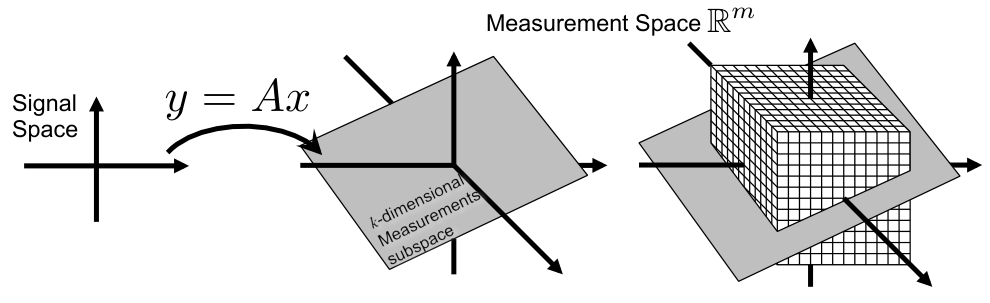
Alternatively, a simpler design approach is the uniform scalar quantizer, which often performs almost as well as an optimal scalar quantizer design. It is significantly less complex and can be shown to approach optimality as the bit-rate increases [39]. The thresholds of a uniform scalar quantizer are defined to be equi-spaced, i.e., , where is referred to as the quantization bin width or resolution. The levels are typically set to the mid-point of the quantization bin . Thus, the quantization error introduced to each coefficient is bounded by . A uniform quantizer defines a uniform grid in the -dimensional measurement space, as shown in Fig. 1.
In practical systems, the scalar quantizer has finite range, i.e., it saturates if the signal exceeds a saturation level . In particular, a uniform finite-range scalar quantizer using bits per coefficient has quantization interval . If a coefficient exceeds , the quantizer maps the coefficient to the largest quantization level, i.e., it saturates. Depending on the magnitude of the coefficient, this may introduce significant error. However, it is often convenient in theoretical analysis to assume an infinite quantizer that does not saturate. This assumption is often justified, as in practice is set large enough to avoid saturation given a signal class. As described in Sec. 3.3, this is often suboptimal in compressive sensing applications.
Compared to classical systems, optimal scalar quantizer designs for compressive sensing measurements require extra care. An optimal design with respect to the measurement error is not necessarily optimal for the signal, due to the non-linear reconstruction inherent in compressed sensing. While specific designs have been derived for very specific reconstruction and probabilistic signal models, e.g., [89, 56], a general optimal design remains an open problem. Thus the literature has focused mostly, but not exclusively, on uniform scalar quantizers.
2.2.2 Scalar Quantization and Oversampling
When a signal is oversampled, a scalar quantizer makes suboptimal use of the bit-rate. The -dimensional signal space mapped through the measurement operator to an -dimensional measurement space, where , spans, at most, a -dimensional subspace of , as shown in Fig. 2. As evident from the figure, this subspace intersects only a few of the available quantization cells and, therefore, does not use the available bits effectively. For an -level quantizer, the number of quantization cells intersected is bounded by [90, 38, 14]
| (13) |
Using a simple covering argument as in Sec. 2.1, it is thus possible to derive a lower bound on the error performance as a function of the number of measurements
| (14) |
The bounds hold for any scalar quantizer design, not just uniform ones.
Linear reconstruction, i.e., reconstruction using a linear operator acting on the scalar quantized measurements, does not achieve the bound (14) [91, 38]. The quantization error using linear reconstruction can only decay as fast as
| (15) |
Instead, consistent reconstruction achieves the optimal bound in a number of cases. Consistent reconstruction treats the quantization regions as reconstruction constraints and ensures that the reconstructed signal quantizes to the same quantization points when measured using the same system. Thus in the oversampled setting where is an matrix with , and where one solves the problem:
| (16) |
If the measurement operator is a tight frame formed by an oversampled Discrete Fourier Transform (DFT), the root mean square error (RMSE) of such a reconstruction (with respect to a random signal model) decays as [91, 38], i.e., as (14). In the case of random frames with frame vectors drawn independently from a Gaussian distribution [50] or from a suitable distribution on the -sphere [84], the reconstruction method in (16) also displays RMSE and worst case reconstruction error decreasing as and , respectively.
The constraints imposed by consistent reconstruction are convex and can be imposed on any convex optimization algorithm. This makes them particularly suitable for a number of reconstruction algorithms already used in compressive sensing systems, as we explore in Sec. 3.
The bounds (14) and (15)—which can be achieved with proper design of the measurement process and the reconstruction algorithm—demonstrate that the most efficient use of the rate is in refining each measurement using more bits per measurement, , rather than in increasing the number of measurements, . They suggest that in terms of error performance, by doubling the oversampling it is possible to save 0.5 bits per coefficient if linear reconstruction is used and 1 bit per coefficient if consistent reconstruction is used. This means that a doubling of the rate by doubling the oversampling factor, is equivalent to a linear increase in the rate by or through an increase in , for linear and consistent reconstruction, respectively. So in principle, if rate-efficiency is the objective, the acquisition system should only use a sufficient number of measurements to reconstruct the signal and no more. All the rate should be devoted to refining the quantizer. However, these bounds ignore the practical advantages in oversampling a signal, such as robustness to erasures, robustness to measurement noise and implementation complexity of high-rate scalar quantizers. Thus in practice, oversampling is often preferred, despite the rate-inefficiency. Techniques such as Sigma-Delta quantization, which we discuss in Sec. 2.3, have been developed to improve some of the trade-offs and are often used in conjunction with oversampling.
2.2.3 Performance Bounds on Sparse Signals
Scalar quantization in compressive sensing exhibits similar bounds as scalar quantization of oversampled signals. Signals that are -sparse in belong to a union of -dimensional subspaces. When measured using linear measurements, they occupy a union of -dimensional subspaces of , of them. Using the same counting argument as above, it is evident that the number of quantization cells intersected, out of the possible ones, is at most
| (17) |
The resulting error bound is
| (18) | ||||
| (19) |
which decays slower than (8) as the rate increases keeping the number of measurements constant. Furthermore, as the rate increases with the number measurements , keeping , the number of bits per measurement constant, the behavior is similar to quantization of oversampled frames: the error can only decay linearly with .
These bounds are not surprising, considering the similarities of oversampling and compressive sensing of sparse signals. It should, therefore, be expected that more sophisticated techniques, such as Sigma-Delta () quantization should improve performance, as they do in oversampled frames. However, their application is not as straightforward. The next section provides an overview of quantization and Sec. 4 discusses in detail how it can be applied to compressive sensing.
2.3 Sigma-Delta Quantization
An alternative approach to the scalar quantization techniques detailed in the previous section is feedback quantization. The underlying idea is that the fundamental limits for the reconstruction accuracy discussed above can be overcome if each quantization step takes into account errors made in previous steps. The most common feedback quantization scheme is quantization, originally introduced for bandlimited signals in [47] (cf. [46]). A simple scheme, illustrated in Figure 3, shows this feedback structure.
A motivation in quantization is that, in some applications, reducing circuit complexity is desirable, even at the expense of a higher sampling rate. Indeed, designs drastically reduce the required bit depth per sample while allowing for accurate signal reconstruction using simple circuits. In fact, since its introduction, quantization has seen widespread use (see, e.g., [77] and the references therein) in applications ranging from audio coding to wireless communication.
Nevertheless, a mathematical analysis of quantization in its full generality has been challenging. A preliminary analysis of simple schemes for restricted input classes (including constant input and sinusoidal input) was presented in [40] and follow-up works. However, most of these results were limited to linear, or at best low-order polynomial error decay in the oversampling rate. This type of error decay is sub-optimal (albeit better than scalar quantization), and rather far from the optimal exponential error decay. Specifically, a major difficulty that prevented a more comprehensive treatment was understanding the instabilities caused by the positive feedback inherent to the circuit designs. For example, depending on the design of the scheme, the state variables could grow without bound. A crucial idea to prevent such phenomena for arbitrary band-limited inputs was developed in [32]; their analysis led, for the first-time, to super-polynomial bounds for the error decay. To date, the best known error bounds decay exponentially in the oversampling rate [41, 35]. While this is near-optimal (optimal up to constants in the exponent), it has been shown that with a fixed bit budget per sample, the achievable rate-distortion relationship is strictly worse than for scalar quantization of Nyquist rate samples [63]. That said, increasing the bit budget per sample entails more expensive and complex circuitry, which grows increasingly costly with every added bit (in fact, the best current quantizers provide a resolution of about 20 bits per sample). Thus, for quantizing bandlimited functions, if one wishes to improve the performance or reduce the cost, one must revert to oversampling-based methods such as quantization.
The accuracy gain of quantization is most prominent when a significant oversampling rate and, therefore, a high redundancy of samples is inherent or desired. Such redundant representations can also be encountered in a finite-dimensional discrete context. Namely, this corresponds to a finite frame expansion in the sense of (1.32). This observation served as a motivation to devise schemes for finite-frame expansions, and the first such construction was provided in [7]. In contrast to oversampled representations of bandlimited signals, which directly correspond to a temporal ordering, finite frames generally do not have an inherent order, nor are the frame vectors necessarily close enough to each other to allow for partial error compensation. Due to this difficulty, the first works on quantization for finite frame expansions focus on frames with special smoothness properties. Namely, they assume that the frame has a well controlled frame variation
The constructions in [7] coupled with (linear) reconstruction via the canonical dual frame (that is, the Moore-Penrose pseudo-inverse of the matrix that generates the redundant representation) was shown to yield an error decay on the order of , i.e., linear error decay whenever the frame variation is bounded by a constant. By using more sophisticated schemes these results were later improved to higher order polynomial error decay [6, 12, 13] in the number of measurements, thereby beating the bound (14) associated with scalar quantization. Again, these constructions require certain smoothness conditions on the frame and employ the canonical dual frame for recovery. In a slightly different approach, the design of the feedback and the ordering of the frame vectors has been considered as part of the quantizer design [20, 14].
A new take on the frame quantization problem was initiated in [65, 10] where the authors realized that reconstruction accuracy can be substantially improved by employing an appropriate alternative dual frame (i.e., , a different left-inverse) for recovery. At the core of this approach is still a smoothness argument, but this time for the dual frame. Given a frame, an appropriate dual frame, the so-called Sobolev dual, can be obtained by solving a least-squares problem over the space of all duals [10]. Again, this yields polynomial error decay, albeit now in more general settings. Moreover, by optimizing over such constructions, root-exponential error decay can be achieved [60].
While the definition of the Sobolev dual does not require any smoothness of the frame, the concrete examples discussed in the aforementioned works still exclusively focused on smooth frames. Similar results on recovery guarantees for frames without smoothness properties were first obtained for frames consisting of independent standard Gaussian vectors [42] and subsequently generalized to vectors with independent subgaussian entries [61].
The underlying constructions also form the basis for the quantization schemes for compressed sensing measurements. Details on such schemes are given in Sec. 4. The insight behind the schemes is that the number of measurements taken in compressed sensing is typically larger than the support size by at least a logarithmic factor in the dimension, and there is an interest in choosing it even larger than that, as this induces additional stability and robustness. Thus, once the support of the signal has been identified and only the associated signal coefficients need to be determined, one is dealing with a redundant representation. The goal is now to employ frame quantization schemes to exploit this redundancy.
For typical compressed sensing matrices, any columns indeed form a frame; this follows for example from the restricted isometry property. However, as the support of the signal is not known when quantizing the measurements, it is crucial that quantization is universal. That is, it must not require knowledge regarding which of a given collection of frames (namely, those forming the rows of an submatrix of ) has been used for encoding. The reconstruction from the resulting digital encodings then typically proceeds in two steps. First the support is identified using standard compressed sensing recovery techniques, just treating the quantization error as noise. In a second step, only the restriction of the measurement matrix to the identified support columns is considered. For the frame consisting of the rows of this matrix, one then applies frame quantization reconstruction techniques. Recovery guarantees for such an approach have been proven for Gaussian measurements [42] and measurements with independent subgaussian entries [61]. It is of great importance that the dual frame used for recovery is chosen properly (e.g., the Sobolev dual), as it follows from the RIP that the frames never have a small frame variation. Here again the recovery error bounds decay polynomially in the number of measurements and beat the analogous bounds for scalar quantization.
Preliminary steps towards a unified approach to support and signal recovery have been considered in [29]. The reconstruction techniques studied in this work, however, intrinsically rely on certain non-convex optimization problems, for which no efficient solution methods are known. Thus the quest remains open for an integrated approach to reconstruction from -quantized compressed sensing measurements that combines numerical tractability and guaranteed recovery.
3 Scalar Quantization and Compressive Sensing
The interplay of scalar quantization and compressed sensing has been widely explored in the literature. In addition to the lower bounds discussed in 2.2.3, there is significant interest in providing practical quantization schemes and reconstruction algorithms with strong performance guarantees.
This part explores these results. Our development considers the following quantized compressed sensing (QCS) model:
| (20) |
where and . The sensing matrix can be, for instance, a random Gaussian sensing matrix such that . Note that the scaling of the entries of the sensing matrix should be independent of . This allows us to fix the design of the scalar quantizer since the dynamic range of the components of is then independent of the number of measurements. This has no consequence on some of the common requirements the sensing matrix must satisfy, such as the Restricted Isometry Property (see Chap. 1), as soon as an appropriate rescaling of is applied. For instance, if has RIP of order and if for some , then has RIP of the same order and the error bound (1.20) in the stability Theorem 1.6 remains unchanged [52].
The first two parts, Sec. 3.1 and Sec. 3.2, focus on the high resolution assumption (HRA) that simplifies the QCS model. Under HRA, the quantization bin widths— or the distance between two consecutive thresholds—are small with respect to the dynamic range of the unquantized input. This allows us to model the quantization distortion as uniform white noise [39]. Determining bounds on its power and moments can better constrain signal reconstruction methods, such as the basis pursuit denoise (BPDN) program [28, 26], which is commonly used for reconstructing signals whose CS measurements are corrupted by Gaussian noise. However, the price to pay is an oversampling in CS measurements.
Sec. 3.3 considers scalar quantizers with saturation. Saturation induces information loss in the measurements exceeding the saturation level. However, democracy—a key property of compressive sensing measurements that makes every measurement equally informative—provides robustness against such corruption.
In Sec. 3.4, very low-resolution quantization is studied through 1-bit compressed sensing. In this case, the HRA cannot be assumed anymore—the quantization bins are the two semi-infinite halves of the real line—and the analysis of the QCS model relies on high dimensional geometric arguments.
Finally, Sec. 3.5 studies how noise, either on the signal or on the measurements, can impact the QCS model (20), the reconstruction error and the quantizer trade-offs. In particular, at constant bit budget , the total noise power determines the optimal trade-off between quantizer precision and number of measurements.
3.1 Uniform Scalar Quantization
First we consider the QCS model (20) using a uniform quantizer with resolution and a set of levels ,
measuring a signal using a sensing matrix . For simplicity, we assume henceforth that is sparse in the canonical basis, i.e., .
We consider a quantizer that has uniform quantization regions, i.e., for all , and, setting , quantization levels in .
By definition, the signal satisfies the following quantization consistency constraint (QCu)
| (QCu) |
From this fact, we can also deduce that
This shows that the QCS model can be assimilated to a noisy CS model
| (21) |
with a “noise” of bounded -norm, i.e., .
The quantization noise power can be further reduced using the high resolution assumption. Under this assumption, the coefficients of may lie anywhere in the quantization region determined by the coefficients of and it is natural to model the quantization distortion as a uniform white noise, i.e.,
Under this model, a simple use of the Chernoff-Hoeffding bound [45] provides, with high probability
for a small constant .
The first approach in modeling and understanding QCS exploited this bound and the development of noise-robust CS approaches to impose a distortion consistency constraint (DCu) [25]
| (DCu) |
on any candidate signal estimating . This was indeed a natural constraint to consider since most noise-robust compressed sensing reconstruction methods can incorporate a bounded -norm distortion on the measurements. For instance, the BPDN program can find a solution of
| (BPDN) |
Then, if the sensing matrix satisfies the RIP with constant on sparse signals, it is known [22] that
where is the best -term approximation defined in (1.2).
This approach has two drawbacks. First, there is no guarantee that the solution satisfies the QCu constraint above, i.e., . This shows that some sensing information has been lost in the reconstruction. Moreover, as described in Sec. 2.2.2, the consistency of the solution helps in reaching the lower bound [38, 84, 50]
in the oversampled setting. Second, from a maximum a posteriori standpoint, since every constrained optimisation corresponds to an unconstrained Lagrangian formulation, imposing a small -norm on the residual can be viewed as enforcing a Gaussian distribution on , which is not the uniform one expected from the HRA.
To circumvent these two limitations, [52] studied the Basis Pursuit DeQuantizer (BPDQp) program
| (BPDQp) |
where must be carefully selected in order for to be a feasible point of this new -constraint. If as , the BPDQp solution tends to be consistent with the quantized measurements. But what is the price to pay, e.g., in terms of number of measurements, for being allowed to increase beyond ?
To answer this, we need a variant of the restricted isometry property.
Definition 1.
Given two normed spaces and (with ), a matrix has the Restricted Isometry Property from to at order , radius and for a normalization , if for all ,
| (22) |
the exponent depending on the spaces and . To lighten notation, we write that is RIP.
In this general definition, the common RIP is equivalent to RIP with (see Chap. 1, Eq. (1.10)). Moreover, the RIP defined in [8] is equivalent to the RIP with , and . Finally, the Restricted -Isometry Property proposed in [27] is also equivalent to the RIP with .
To characterize the stability of BPDQ we consider the space and with , and we write RIPp as a shorthand for RIP. At first sight, it could seem unnatural to define an embedding of in for , those spaces being not isometrically isomorphic to each other for . However, the RIPp rather sustains the possibility of an isometry between and . We will see in Prop. 1 that the existence of such a relation comes with an exponential growth of as increases, a phenomenon that can be related to Dvoretsky’s theorem when specialized to those Banach spaces [69].
From this new characterization, one can prove the following result.
Theorem 1 ([52, 53]).
Let , and be a RIP matrix for and some normalization constant . If
| (23) |
then, for any signal observed according to the noisy sensing model with , the unique solution obeys
| (24) |
where, again, denotes the best -term approximation.
This theorem follows by generalizing the fundamental result of Candès in [26] to the particular geometry of Banach spaces . It shows that, if is RIPp with particular requirement on the RIPp constant, the BPDQp program is stable under both measurement noise corruption and departure from the strict sparsity model, as measured by . In particular, under the same conditions, given a measurement noise and some upper bounds on its -norm, (24) provides the freedom to find the value of that minimizes .
This is exactly how QCS signal recovery works. Following Theorem 1 and its stability result (24), we jointly determine a RIPp sensing matrix with known value and a tight error bound on the norm of the residual under HRA. The existence of a RIPp matrix is guaranteed by the following result [52, 53].
Proposition 1 (RIPp Matrix Existence).
Let a random Gaussian sensing matrix be such that , and . Then, is RIP with probability higher than when we have jointly and
| (25) |
Moreover, .
There is thus an exponential price to pay for a matrix to be RIPp as increases: roughly speaking, for , we need measurements for satisfying this property with non-zero probability.
To estimate a tight value of in the case of quantization noise—since, under HRA —we can show that
| (26) |
with probability higher than . Actually, for , is a feasible solution of the BPDQp fidelity constraint with a probability exceeding .
Finally, combining the estimation with the bound on , we find, under the conditions of Prop. 1,
| (27) |
This shows that, in the high oversampled sensing scenario driven by (25), and provided the RIPp constants satisfy (23), the part of the reconstruction error due to quantization noise behaves as . This is also the error we get if is exactly -sparse since then vanishes in (24).
If we solve for , we can see that the error decays as as increases. There is possibly some room for improvements since, as explained in Sec. 2.2.2, the lower bound on reconstruction of sparse signal is . Beyond scalar quantization schemes, Sec. 4 will also show that much better theoretical error reduction can be expected using quantization.
Interestingly, we can, however, observe a numerical gain in using BPDQp for increasing values of when the signal is observed by the model (21) and when increases beyond the minimal value needed for stabilizing BPDN (i.e., BPDQ2).
This gain is depicted in Fig. 4. The plots on the left correspond to the reconstruction quality, i.e., the value expressed in dB, reached by BPDQp for different values of and . The original signal has dimension and is -sparse in the canonical basis, with support of size uniformly random and normally distributed non-zero coefficients. Each point of each curve represents average quality over 500 trials. For each sparse signal , quantized measurements were recorded using (21) with a random Gaussian sensing matrix and . The reconstruction was done by solving BPDQp with the Douglas-Rachford algorithms [52], an efficient convex optimization method solving constrained programs, such as BPDQ11 1 The code of BPDQ is freely available at http://wiki.epfl.ch/bpdq., using simpler proximal operators [30]. Fig. 4(a) shows that higher oversampling ratio allows the use of higher with significant gain in the reconstruction quality. However, if is low, i.e., close to , the best quality is still reached by BPDN. The quantization consistency of the reconstruction, i.e., the original motivation for introducing the BPDQp program, can also be tested. This is shown on Fig. 4(b) and Fig. 4(c) where the histograms of the components of are represented for and at . This histogram for is indeed closer to a uniform distribution over , while the one at is mainly Gaussian.
3.2 Non-Uniform Scalar Quantization
If the distribution of the measurements is known, quantization distortion can be decreased by adopting a non-uniform scalar quantizer. For instance, when is a random Gaussian matrix viewing the signal as fixed and the matrix as randomly drawn, the distribution of the components of is also Gaussian with a variance proportional to the signal energy (and similarly, for other matrix constructions, such as ones drawn with random sub-Gaussian entries). Assuming the acquired signal energy can be fixed, e.g., using some automatic gain control, the known distribution of the measurements can be exploited in the design of the quantizer, thanks for example to the Lloyd-Max algorithm mentioned in Sec. 2.2 [71]. In particular, the quantization thresholds and levels are then optimally adjusted to this distribution.
This section shows that the formalism developed in Sec. 3.1 can indeed be adapted to non-uniform scalar quantizer. To understand this adaptation, we exploit a common tool in quantization theory [39]: any non-uniform quantizer can be factored as the composition of a “compression” of the real line over followed by a uniform quantization of the result that is finally re-expanded on . Mathematically,
| (28) |
where is the compressor and is the expander, giving the name compander as a portemanteau.
In particular, under HRA, the compressor of a distortion optimal quantizer, i.e., one that minimizes for a source modeled as a random variable with pdf , must satisfy
and if is an optimal -bit quantizer (e.g., obtained by Lloyd-Max method) then in (28). In this case, the Panter and Dite formula estimates the quantizer distortion as [79]
with -norm and where “” means that the relation tends to an equality when is large. The rest of this section assumes that the expected distribution is Gaussian, i.e., if and , as it comes by seeing the signal fixed (with known energy) and the Gaussian matrix random in CS.
Compander theory generalizes quantization consistency in the “compressed” domain, i.e.,
Therefore, for the right compressor , in the noiseless QCS model (20), the signal provides consistency constraints to be imposed on any reconstruction candidate :
| (QC) |
This generalizes the uniform quantization consistency (QCu) introduced in Sec. 3.1.
The compander formalism is leveraged in [53], to generalize the approach described in Sec. 3.1 to non-uniform quantization. In particular, a new set of parametric constraints are introduced, the -Distortion Consistency (or DpC) for . These have for limit cases the QC above and the distortion consistency constraint (DC) arising from Panter and Dite formula, namely, the constraint imposing any reconstruction candidate to satisfy [31]
| (DC) |
with DC asymptotically satisfied by when both and are large.
The DpC constraint corresponds to imposing that a candidate signal satisfies
| (DpC) |
where is the weighted -norm of with weights , denoting by the diagonal matrix having on its diagonal. The mapping is a post-quantization modification of characterized componentwise hereafter and such that .
Under HRA, a careful design of , and the bounds ensures that D2C amounts to imposing DC on and, that as , DpC tends to QC [53]. Briefly, if falls in the quantization bin , is defined as the minimizer of
Actually, by equivalence with (12), and . The weights are defined by the quantizer compressor with . Moreover, under HRA and asymptotically in , an optimal bound reads . For , matches the distortion power estimated by the Panter and Dite formula, while for , , i.e., half the size of the uniform quantization bins in the domain compressed by .
Similarly to Sec. 3.1, using (DpC) as a fidelity constraint in the signal reconstruction leads to the definition of a Generalized Basis Pursuit DeNoise program:
| (GBPDN) |
Ideally, we would like to directly set in order to enforce consistency of with . However, as studied in [53], it is not certain that this limit case minimizes the reconstruction error as a function of , given a certain number of measurements .
Actually, the stability of GBPDN can be established from the one of BPDQ (Sec. 3.1) if we impose to satisfy the more general RIP, as formally defined in (22). Indeed, for any weighting vector , we have always with and . Therefore, we know from Theorem 1 that if is RIPp, or equivalently if is RIP, with the additional condition (23) on its RIP constants at different sparsity levels, then the solution of GBPDN will be stable in the sense of (24), i.e.,
Compared to the unit weights case (as involved by the RIPp), a random Gaussian matrix with satisfies the RIP with high probability provided that grows like . The ratio depends on the conditioning of . It is equal to 1 for constant weights (recovering (25)), while it increases with the dynamic range of . For the weight defined previously and with a Gaussian optimal quantizer, asymptotically in and .
As for the uniform case, a strong (polynomial) oversampling in is thus required for satisfying the RIP at compared to the minimal number of measurements needed at . However, an asymptotic analysis of shows that the GBPDN reconstruction error due to quantization for a Gaussian sensing matrix behaves like [53]
This error decay is thus similar to the one found in (27) for uniform QCS with now a direct interpretation in terms of the quantizer bit-depth .
Efficient convex optimization methods, like those relying on proximal algorithms [30], can also be used to numerically solve GBPDN. In [53], numerical simulations show that the reconstruction qualities reached in the reconstruction of sparse signals from their non-uniformly quantized measurements behave similarly, with respect to and , to those observed in Sec. 3.1 for the uniformly quantized CS setting.
3.3 Finite-Range Scalar Quantizer Design
So far we have only considered a scalar quantizer model without saturation. Practical scalar quantizers have a finite range, which implies a saturation level and, using bits per coefficient, a quantization interval equal to
| (29) |
In order to determine the optimal saturation rate, the system designed needs to balance the loss of information due to saturation, as decreases, with the increased quantization error due to an increasing quantization interval in (29), as increases. In classical systems, this balance requires setting the quantization level relatively close to the signal amplitude to avoid saturation. On the other hand, in compressive sensing systems, the incoherence of the measurements with the sparsity basis of the signal makes them more robust to loss of information and enables higher saturation levels with smaller quantization intervals.
A key property of compressive measurements, which provides the robustness to loss of information, is democracy. Intuitively, each measurement contributes an equal amount of information to the reconstruction. If the signal is slightly oversampled, relative to the rate required for CS reconstruction, then any subset with enough measurements should be sufficient to recover the signal. The notion of democracy was first introduced in [23, 43] in the context of information carried in each bit of the representation; the definition below strengthens the concept and formulates it in the context of compressive sensing [33, 66].
Definition 2.
Let , and let be given. We say that is -democratic if, for all row index sets such that , any matrix , i.e., comprised of a -subset of the rows of , satisfies the RIP of order with constant .
This definition takes an adversarial view of democracy: a matrix is democratic if an adversary can pick any rows to remove from , and the remaining matrix still satisfies the RIP. This is a much stronger guarantee than just randomly selecting a subset of the rows to be removed. Such a guarantee is important in the case of saturation robustness because the saturated measurements are the largest ones in magnitude, i.e., potentially the ones most aligned with the measured signal and, presumably, the ones that capture a significant amount of information. Still, despite this strict requirement, randomly generated matrices can be democratic if they have a sufficient number of rows.
Theorem 2 ([33]).
Let with elements drawn according to and let , , and be given. Define . If
| (30) |
then with probability exceeding we have that is -democratic, where is arbitrary and
The practical implication of democratic measurements is that information loss due to saturated measurements can be tolerated.
Saturated measurements are straightforward to detect, since they quantize to the highest or the lowest level of the quantizer. The simplest approach is to treat saturated measurements as corrupted, and reject them from the reconstruction, together with the corresponding rows of . As long as the number of saturated measurements is not that large, the RIP still holds and reconstruction is possible using any sparse reconstruction algorithm.
However, saturated measurements do contain the information that the measurement is large. In the context of consistent reconstruction, they can be used as constraints in the reconstruction process. If a measurement is positively saturated, then we know that . Similarly, if it is negatively saturated, . These constraints can be imposed on any reconstruction algorithm to improve performance [66].
| (a) | (b) | (c) |
Fig. 5 demonstrates the effect of each approach. As demonstrated in the plots, rejecting saturated measurements or treating them as consistency constraints significantly outperforms just ignoring saturation. Furthermore, if saturation is properly taken into account, a distortion optimal finite-range scalar quantizer should be designed with significant saturation rate, often more than 20%. While the figures suggest that saturation rejection and saturation consistency have very similar performance, careful examination demonstrates, as expected, that consistency provides more robustness in a larger range of saturation rates and conditions. A more careful study and detailed discussion can be found in [66]. Furthermore, further gains in the bit-rate can be achieved by coding for the location of the saturated measurements and transmitting those separately [58].
3.4 1-Bit Compressive Sensing
The simplest scalar quantizer design to implement in hardware is a 1-bit quantizer, which only computes the sign of its input. Its simplicity makes it quite appealing for compressive sensing systems.
The sensing model of 1-bit CS, first introduced in [19], is very similar to the standard scalar quantization model
| (31) |
where is a scalar function applied element-wise to its input and equals if and otherwise.
One of the challenges of this model is that it is invariant under changes of the signal amplitude since for any positive . For that reason, enforcing consistency is not straightforward. A signal can be scaled arbitrarily and still be consistent with the measurements. Thus, a magnitude constraint is typically necessary. Of course, the signal can only be recovered within a positive scalar factor.
Similarly to multi-bit scalar quantization models, the literature in this area focuses on deriving lower bounds for the achievable performance, reconstruction guarantees, as well as practical algorithms to invert this problem.


3.4.1 Theoretical Performance Bounds
A lower bound on the achievable performance, can be derived using a similar analysis as in Sec. 2.2.3. The main difference is that the quantization cells are now orthants in the -dimensional space, shown in Fig. 6(a), corresponding to each measured sign pattern. Each subspace of the possible ones intersects very few of those orthants, as shown in Fig. 6(b), i.e., uses very few quantization points. In total, at most quantization cells are intersected by the union of all subspaces [54].
Since the signal amplitude cannot be recovered, the lower bound is derived on -dimensional spheres and coverings using spherical caps instead of balls. The derivation ensures that the spherical caps have radius sufficiently large to cover the spheres. Despite the similarity to the argument in Sec. 2.2.3, this case requires a little bit more care in the derivation; details can be found in [54]. Still, the result is very similar in nature. Defining we have:
Theorem 3 ([54]).
Given , any estimation of obtained from has a reconstruction error of at least
which is on the order of as increases.
If the sensing matrix is Gaussian, i.e., if , any -sparse signal that has consistent measurements will not be very far from the signal producing the measurements, assuming a sufficient number of them. This guarantee approaches the lower bound of Theorem 3 within a logarithmic factor.
Theorem 4 ([54]).
Fix and . If the number of measurements is
| (32) |
then for all we have that
| (33) |
with probability higher than . Equivalently, if and are given, solving for above leads to
| (34) |
with the same probability.
Fig. 6(c) provides further intuition on these bounds by illustrating how 1-bit measurements operate in the signal space. Specifically, each measurement corresponds to a hyperplane in the signal space, orthogonal to the measurement vector. The measurement sign determines on which side of the hyperplane the signal lies. Furthermore, the signal is sparse, i.e., lies in . A consistent sparse reconstruction algorithm can produce any sparse signal in the indicated shaded region.
A new measurement provides new information about the signal only if the corresponding hyperplane intersects the region of consistent signals and, therefore, shrinks it. However, as more measurements are obtained and the consistency region shrinks, newer measurements have lower probability of intersecting that region and providing new information, leading to the decay of the error.
Consistency can be quantified using the normalized hamming distance between measurements
where denotes the exlusive-OR operator. It is, thus, possible to show that if and above differ by no more than bits in their 1-bit measurements, i.e., if , then, with and with high probability [51],
A bound similar to (34) exists for sign measurements of non-sparse signals in the context of quantization using frame permutations [76]. In particular, reconstruction from sign measurements of signals exhibits (almost surely) an asymptotic error decay rate arbitrarily close to . However, in contrast to Theorem 4 this result holds only for a fixed signal and not uniformly for all signals of interest.
Note that these results focus on matrices generated using the normal distribution. It has been shown that matrices generated from certain distributions do not perform well in this setting, even though they can be used in standard compressive sensing [82]. For instance, consider a random Bernoulli matrix such that or with equal probability. In this case, the two distinct sparse vectors and with are apart and they generate the same quantization vector , where is the first column of . It is not possible, therefore, to distinguish those two vectors from their 1-bit observations by increasing and guarantee that the reconstruction error will decay as measurements increase. This counterexample, however, is exceptional in the sense that such failures can only happen if the signal can have a very large entry. Under mild flatness assumptions on the -norm of the signal, arbitrary subgaussian measurements can be utilized [1].
These results establish lower and upper bounds on distances between two sparse signals that have (almost) consistent 1-bit measurements. It is also possible to provide an embedding guarantee similar to the RIP [25]. Since the measurement does not preserve the signal magnitude, we should not expect distances of signals to be preserved. However, the measurements do preserve angles between signals. Defining we have:
Theorem 5 (Binary -Stable Embedding (BSE) [54]).
Let be a random Gaussian matrix such that . Fix and . If the number of measurements satisfies
| (35) |
then with probability exceeding
| (36) |
for all .
In other words, up to an additive distortion that decays as , the Hamming distance between and tends to concentrate around the angular distance between and . Notice that, in contrast to the RIP, a vanishing distance between the quantized measurements of two signals does not imply they are equal, i.e., we observe a (restricted) quasi-isometry between and instead of the common RIP [49]. This comes from the additive nature of the distortion in (36) and is a direct effect of the inherent ambiguity due to quantization.
This embedding result has been extended to signals belonging to convex sets provided that their Gaussian mean width
| (37) |
with , can be computed [80, 81, 82]. In particular, if
for some constant , then (36) holds with high probability for any . In particular, for
since [81], an embedding exists between the set of compressible vectors modeled by and provided that .
Note that generalizations of these embeddings to non-linear functions other than the operator, or to stochastic processes whose expectation is characterizable by such functions, are also possible [81].
3.4.2 Reconstruction from 1-Bit Measurements
The original efforts in reconstructing from 1-bit measurements enforced as a reconstruction constraint, formulating the non-convex minimization problem
| (38) |
Even though the problem is not convex, a number of algorithms have been shown experimentally to converge to the solution [19, 67]. More recently, a number of greedy algorithmic alternatives have also been proposed [15, 3, 54].
Most of these algorithms attempt to enforce consistency by introducing a one-sided penalty for sign violations
| (39) |
where is the element-wise product between vectors, if is negative and 0 otherwise, also applied element-wise, and the norm is typically the or the norm. Typically, a descent step is performed using the gradient of (39), followed by a support identification and sparsity enforcement step. Often, care is taken in selecting the descent step, especially considering the signal is on the unit sphere [67]. Assuming a certain noise level, a maximum likelihood formulation can also be used to remove the norm constraint [3].
For example, the Binary IHT (BIHT), a variation of the popular Iterative Hard Thresholding (IHT) [11], uses the one-sided norm in (39) and follows its subgradient . The algorithm is defined by the iteration
| (40) |
where is a hard threshold, keeping the largest coefficients of its input and setting the remaining ones to zero.
The BIHT does not have convergence or reconstruction guarantees to a consistent output. Still, as shown in Fig. 7, it works surprisingly well compared to other greedy approaches. Moreover, variations exist to make it more robust to potential binary errors in the knowledge of [54] or to extend it to multi-bit scalar quantization [51].
The first iteration of BIHT is a simple truncated back-projection, whose distance to is known to decay asymptotically as for a Gaussian matrix [51, 3]. Furthermore, matches the solution of the (feasible) problem
where maximizing also promotes the 1-bit consistency of with .
This optimization can be generalized to any convex sets where can lie, such as the set of compressible signals with Gaussian width [81]. If for some , and a fixed is sensed using (31) with a Gaussian sensing matrix , then the solution to
satisfies with high probability. Interestingly, under certain conditions, this holds also for sensing models other than (31), where the sign operator is replaced, for instance, by the logistic function [81].
What makes it difficult to provide reconstruction error estimates for algorithms motivated by the problem (38) is the non-convex constraint , whose convex relaxation allows for the zero solution and is hence meaningless. To overcome this obstacle, it has been proposed in [80, 81] to impose a norm constraint to prevent trivial solutions on the measurements rather than the signal. This results in a different problem, which allows for a meaningful convex relaxation. Namely, since , it follows that at the solution . Thus, by constraining this norm, the following convex problem can be formulated:
| (41) |
As shown in [80], the problem in (41) does allow for reconstruction guarantees: If , the solution recovered from quantized Gaussian measurements of a sparse signal is such that with high probability. This holds uniformly for all signals . Under flatness assumptions on the signal, recovery guarantees can also be proved for arbitrary subgaussian measurements [1].
3.5 Noise, Quantization and Tradeoffs
The sections above were focused on noiseless QCS models. These models only consider the statistical or the geometrical properties of quantization of CS measurements under high or low resolution modes. However, any signal acquisition system is subject to noise corruption before quantization, either on the measurement process or on the signal itself. Such noise can be incorporated in a more general model
| (42) |
where and corrupt the signal and the sensing, respectively, before quantization. Examining the impact of such noise in signal recovery leads to new interesting questions.
In [93] two efficient reconstruction methods are developed for sparse or compressible signals sensed according (42) under sensing noise only, i.e., . The two approaches are mainly numerical: one relies on a maximum likelihood formulation, built on the quantization model and on a known Gaussian noise distribution, the other follows a least square principle. The two resulting methods are both regularized by an -norm accounting for sparse signal prior. A provably convergent procedure inherited from a fixed point continuation method is used for reconstructing the signal in the two possible frameworks. With their approach, the combined effects of noise and coarse quantization can be jointly handled. Reasonable reconstruction results are achieved even using 1 or 2 bits per measurement.
The case , boils down to an interaction of the well-understood phenomenon of noise folding in CS [34] and quantization [68]. Noise-folding in unquantized CS says that under a weak assumption of orthogonality between the rows of , the variance of the component undergoes a multiplication by compared to the variance of . This impacts directly the reconstruction error of signals. The corresponding MSE is then times higher than the noise power, or equivalently, the SNR looses 3 dB each time is divided by 2 [34].
An extension of this result to noisy QCS has been provided in [68], assuming the sensing matrix is RIP of order and constant . In this case, if is standard normally distributed and if the quantizer has resolution , then, under a random signal model where the signal support is chosen uniformly at random in and the amplitudes of the non-zero coefficients are standard normally distributed,
| (43) |
where is the oracle-assisted reconstruction of knowing the support of for each of its realization, and
measures the worst correlation between distinct quantized measurements.
In (43), the first term accounts for the quantization error of the signal itself, while the second term represents both the error due to folded signal noise as well as the quantization of that noise. Finally, the third term reflects a distortion due to correlation between quantized measurement. It is expected to be negligible in CS scenarios, specially when increases or if a dithering is added to [39].
| (a) dB, optimal bit-depth | (b) dB, optimal bit-depth |
| (c) dB, optimal bit-depth | (d) dB, optimal bit-depth |
Numerical study of (43) shows that, at constant rate , a tradeoff can be expected between a measurement compression (MC) regime, where is small (but still high enough to guarantee to be RIP) and is high, and a quantization compression (QC) regime, where is high compared to the standard CS setting but is small. Interestingly, the optimal bit-depth , minimizing the expected reconstruction error, depends on the input SNR: . This is illustrated in Fig. 8 where the evolution of (43) (discarding the effect of the third term) is plotted for four different noise scenarios. The optimal bit depth decays smoothly with the ISNR, suggesting that the QC regime is preferable at low ISNR while MC is clearly better at high ISNR. The general behavior of Fig. 8 is also confirmed on Monte Carlo error estimation of the oracle-assisted reconstruction defined above [68].
4 Sigma-Delta Quantization for Compressive Sensing
As mentioned in the introduction, quantization for compressed sensing fundamentally builds on corresponding schemes for finite frames. Thus before presenting an analysis specific to compressed sensing, we first discuss the finite frame case.
4.1 Quantization for Frames
Let with columns be a frame in the sense of (1.32) and consider the frame expansion
of a signal . The goal is now to quantize as a whole such that the quantized representation allows for approximate recovery of . quantization schemes obtain such a using a recursive procedure, which we will now explain in detail.
At the core of the schemes is a uniform scalar quantizer , which maps a real number to the closest point in a codebook of the form
| (44) |
A scheme applies such a quantizer sequentially to the entries of , taking in each quantization step the errors made in previous steps into account. The complexity parameter is referred to as the order of the scheme; it quantifies the trade-off between required storage and achievable accuracy.
A first order quantization scheme, the simplest such algorithm, hence retains the error only for one step. In the following formalization associated with the so-called greedy first order scheme, the error parameter appears as the state variable ; it measures the total accumulated error up to step . The quantized frame coefficient vector is computed by running the iteration
| (45) |
As initialization, one typically uses . In matrix-vector notation, the above recurrence relation reads
| (46) |
Here is the finite difference matrix with entries given in terms of the Kronecker delta by , that is,
| (47) |
The scheme is explicitly designed such that each partly cancels the error made up to . When the signal is approximated as using a dual frame with columns , this entails that one seeks to compensate an error in the direction of a dual frame vector using a distortion in the direction of the next dual frame vector . This serves as a motivation to choose a smoothly varying dual frame, i.e., with subsequent dual frame vectors close to each other.
Bounding the reconstruction error using (46) in terms of the operator norm , one obtains
The smoothness intuition is reflected in the fact that the columns of are given by Thus more precisely, finding a smooth dual frame amounts to minimizing .
If one is willing to store more than one previous value of the state variable, that is, to consider a higher order scheme, it is possible to profit from higher order smoothness of the dual frame. Such a generalization of (45) is the greedy -th order scheme, which is associated with the recurrence relation
| (48) |
Here, the iteration to compute the quantized coefficients is explicitly given by
| (49) |
As before, one initializes . The reconstruction error is now bounded by
| (50) |
Examining (50), it is advantageous to choose a dual frame that minimizes , and a scheme that yields a state-variable sequence with well bounded . This motivates the following definitions.
Definition 3.
Let be a frame and be a positive integer. Then the -th order Sobolev dual of is given by
| (51) |
where the minimum is taken over all dual frames of .
Definition 4.
A scheme with a codebook is stable if there exist constants and such that whenever we have
In general, designing and proving the stability of quantization schemes of arbitrary order can be quite difficult if the number of elements in the associated codebook is held fixed. This challenge is especially difficult in the case of 1-bit quantizers and overcoming it is the core of the contributions of [32, 41, 35], where stable quantization schemes of arbitrary order are designed. On the other hand, if the number of elements in the codebook (44) is allowed to increase with order, then even the simple greedy schemes (49) are stable, as the following proposition shows (see, e.g., [13]).
Proposition 2.
Proof.
Working with stable -th order schemes and frames with smoothness properties, and employing the Sobolev dual for reconstruction, it was shown in [10] that the reconstruction error satisfies , where the constant depends only on the quantization scheme and the frame. Such results for -quantization show that its error decay rate breaks the theoretical lower bound of scalar quantization described in the introduction. Fig. 9 helps to illustrate why such a result is possible. It shows the quantization cells associated with two bit quantization of , where in the unit ball of , using both first order quantization and scalar quantization. For vectors belonging to a given cell, the worst case error achieved by an optimal decoder is proportional to the diameter of the cell. The figure shows that the cells resulting from quantization are smaller than those resulting from scalar quantization, indicating the potential for a smaller reconstruction error. For a detailed overview of quantization of frame expansions see, e.g., [83].
 |
 |
The existing recovery algorithms for quantized compressed sensing measurements rely on a two stage algorithm. In the first stage, the signal support is recovered and in the second stage, the signal coefficients are estimated using the Sobolev dual of the frame associated with the recovered support.
4.2 Finding the Signal Support
Let be the -th order quantization of the compressed sensing measurements associated with the sparse vector and the measurement matrix . In order to preserve the codebook definition (44), we assume as in Sec. 3 that the scaling of the entries of is independent of .
The goal of the first stage of the reconstruction algorithm is to recover . To that end, following [42] we will use a (standard) compressed sensing decoder that has uniform robustness guarantees for matrices with an appropriate RIP constant. For such a decoder and an arbitrary scalar
| (53) |
For example, if is the output of an -minimization algorithm such as Basis Pursuit DeNoising (BPDN), it satisfies (53) with constant when the matrix (more precisely ) satisfies an appropriate restricted isometry property [26]. As the next proposition shows, robust decoders allow recovering the support of a sparse vector when its smallest non-zero entry is above the error level.
Proposition 3.
Let be a compressed sensing decoder satisfying (53) and let with . Define . If then the largest coefficients of are supported on .
Proof.
First, note that for all , (53) yields . Since , the reverse triangle inequality gives for all in . On the other hand, (53) also ensures that for all .
A sharper version of this argument appears in [42] but Proposition 3 is sufficient for our purposes. In particular, consider an th order greedy quantization associated with a codebook having elements. Applying such a scheme to yields a quantized vector satisfying provided
| (54) |
Thus assuming that has appropriate RIP constants, Proposition 3 shows that using a decoder satisfying (53), the support of can be accurately recovered provided for all . What remains is to choose the number of levels in the codebook to satisfy (54); this in turn requires an estimate of .
To that end, we now consider subgaussian measurement matrices, i.e., matrices whose entries are subgaussian random variables as defined below.
Definition 5.
Let be a Gaussian random variable drawn according to . If a random variable satisfies for all , then we say is subgaussian with parameter .
Examples of subgaussian random variables include Gaussian, Bernoulli, and bounded random variables, as well as their linear combinations. For matrices populated with such subgaussian entries, the following proposition from [61] gives a bound on when the non-zero entries of are restricted to a fixed support so that for a frame associated with the support.
Proposition 4.
Let be a subgaussian matrix with mean zero, unit variance, and parameter , where . Let and fix . Then, with probability at least , we have for all and
| (55) |
Here is a constant that may depend on , but is independent of and .
Taking a union bound over all the submatrices of of size yields an identical uniform bound on , which holds for sparse vectors with high probability, provided .
Thus an -th order greedy scheme with sufficiently many quantization levels allows the recovery of a sparse signal’s support from its compressed sensing measurements. Equipped with this knowledge, we can estimate the signal coefficients using the Sobolev dual of the frame associated with the recovered support.
∎
4.3 Recovering the Signal Coefficients
We continue to consider Gaussian or subgaussian measurement matrices, now assuming that the support of the signal has been identified. Our goal is to approximate the coefficients , . With high probability, the matrix has the restricted isometry property of order and level provided one takes at least on the order of measurements. Then the matrix restricted to the columns indexed by is close to an isometry and its rows hence form a frame. Consequently, the measurement vector is the associated frame expansion of , and is the corresponding frame quantization.
As shown in Sec. 4.1, it is advantageous to reconstruct from the -th order quantization of the measurement vector using the Sobolev dual of , see (50) and (51). A possible bound for the reconstruction error is then proportional to . Thus to show a uniform recovery guarantee, one needs a bound for this quantity which is uniform over all potential support sets . In the initial work [42], dealing with Gaussian compressed sensing matrices, the approach to proving such a bound consisted of explicitly controlling the lowest singular value of . Their approach utilized the unitary invariance of the Gaussian measure to identify the distribution of the singular values of the random matrix with those of , where is a diagonal matrix whose entries are the singular values of , and is a Gaussian matrix. This, coupled with bounds on the singular values of , allowed [42] to derive bounds that held with probability high enough to survive a union bound over all Gaussian submatrices of . In [61], this approach was extended to subgaussian matrices. Herein, to prove such a bound on , we follow the simpler, RIP-based approach presented in [37].
To that end, let be the singular value decomposition (SVD) of any matrix (for some orthogonal matrices and ) where the matrix is diagonal with (ordered) diagonal entries . We denote also the smallest singular value of . Then the following proposition (see, e.g., [42]) holds.
Proposition 5.
There are positive constants and , independent of , such that
| (56) |
Denote by the matrix that maps a vector to its first components. Moreover, denote by the set of -sparse signals whose support can be recovered from with the decoder as in Proposition 3. The following theorem describes the reconstruction performance.
Theorem 6 ([37]).
Let be a matrix such that for a fixed , the matrix has restricted isometry constant . Then the following holds uniformly for all .
If has support , is the -th order quantization of , and , then
where is a constant depending only on r and is the quantization step size.
Proof.
The above theorem can be applied almost directly to Gaussian compressed sensing matrices. If is a Gaussian matrix with independent zero mean and unit variance entries, then by rotation invariance so is the matrix . Regarding the choice of , note from Theorem 6 that the smaller is, the better the bound. On the other hand has to be large enough for to have the restricted isometry constant . This prompts the choice , as then has the restricted isometry constant with high probability, as discussed in Chapter 1 (see, e.g., Theorem 1.5). In particular, if
and
then
Applying Theorem 6 directly, we obtain
This essentially recovers the result in [42] and a similar, albeit more technical argument for subgaussian matrices, using either bounds on tail probabilities for quadratic forms [44, 87] or bounds for suprema of chaos processes [59] recovers the analogous result in [61].
To illustrate the advantage of using schemes for quantizing compressed sensing measurements we conduct a numerical experiment with -sparse signals in , as we vary the number of measurements . We fix and the quantization step-size . We draw Gaussian matrices for and quantize the measurements using scalar quantization and th order schemes with . We then use the two-stage reconstruction method described herein to obtain an approximation of using its quantized measurements. Repeating this experiment 30 times, we compute the average of the reconstruction error for each of the quantization methods and plot them against the oversampling ratio in Fig. 10.
In summary, using Gaussian and subgaussian compressed sensing matrices recovery of sparse signals from their quantized measurements is possible. More importantly, the reconstruction error decays polynomially in the number of measurements and thus outperforms the (at best) linear error decay that can be achieved with scalar quantization. This improvement comes at the cost of introducing memory elements, and feedback, into the quantization procedure.
5 Discussion and Conclusion
Quantization is an essential component of any acquisition system, and, therefore, an important part of compressive sensing theory and practice. While significant work has been done in understanding the interaction of quantization and compressive sensing, there are several open problems and questions.
One of the most interesting open problems is the interaction of quantization with noise. While the discussion and references in Sec. 3.5 provides some initial results and theoretical analysis, a comprehensive understanding is still missing. An understanding of the optimal bit allocation and the optimal quantizer design, uniform or non-uniform scalar, or , given the noise level, as well as the robustness of the reconstruction to noise and quantization is still elusive.
While can be used to improve the rate efficiency of compressive sensing, compared to scalar quantization, the performance is still not comparable to the state-of-the-art in conventional methods. For example, conventional quantization of band-limited functions can achieve error that decays exponentially as the sampling rate increases, not currently possible with existing compressive sensing . Furthermore, the analysis in Sec. 4 does not hold for 1-bit quantization, often desirable in practical systems due to its simplicity. Such an extension has significant practical importance.
Even with approaches, the rate efficiency of compressive sensing systems is not ideal. As evident from the fundamental bounds in Sec. 2, compressive sensing is not rate-efficient compared to classical methods such as transform coding. In others word, while compressive sensing is very promising in building sensing systems because it can significantly reduce the number of measurements and the sampling burden, it is not a good data compression approach if the measurements have already been obtained and the achievable bit-rate is important. That said, due to the intimate connection between frame quantization and quantization for compressed sensing, promising results in the finite frames context, e.g., [48] can inform future developments in compressed sensing.
The potential encoding simplicity of a compressive sensing system is very appealing. Acquiring generalized linear measurements and quantizing them can be less complex than typical transform-coding approaches and much more attractive in low-power and computationally-restricted sensing applications. The complexity is shifted to the reconstruction, which, in many applications, can bear significantly more computational complexity. Nevertheless, the rate inefficiency of compressive sensing can be a barrier in such applications.
A number of promising approaches have been proposed to overcome this barrier using modifications of the quantizer that produce non-contiguous quantization regions [78, 16, 17, 57]. Initial theoretical analysis and experimental results are promising. However, our understanding is still limited. One of the drawbacks of such approaches is that the reconstruction is no longer convex and, therefore, not as simple to provide guarantees for.
Alternatively, recent work on adaptive quantization strategies has shown that error decay exponential in the bit-rate can be achieved, even using a 1-bit quantizer, at the cost of adaptivity in the measurements and – in contrast with the methods presented in this chapter – significant computation at the encoder. Specifically, [5] shows that adaptively choosing the threshold of a 1-bit quantizer allows the error to decay exponentially with the number of measurements. The cost is that the thresholds are updated by solving an minimization problem, or running an iterative hard thresholding scheme. It is thus interesting to quantify the tradeoff between computational complexity at the quantizer, and achievable reconstruction accuracy.
Another important aspect is that while the best recovery guarantees in compressed sensing are obtained for Gaussian and subgaussian measurement matrices, which are also mainly considered in this article, applications usually require structured matrices, such as subsampled Fourier matrices, e.g., as a model for subsampled MRI measurements [72], or subsampled convolution, e.g., as a model for coded aperture imaging [73]. In both cases, when the subsampling is randomized, near-optimal recovery guarantees are known for unquantized compressed sensing [86, 59]. Combined with quantization, however, hardly anything is known for such matrices. Such results would be of great importance to move the approaches discussed in this survey closer to the application scenarios.
Quantization is also important when considering randomized embeddings, an area of research intimately related to compressive sensing [4, 62]. Embeddings are transformations that preserve the geometry of the space they operate on; reconstruction of the embedded signal is not necessarily the goal. They have been proven quite useful, for example, in signal-based retrieval applications, such as augmented reality, biometric authentication and visual search [70, 21, 85].
These applications require storage or transmission of the embedded signals, and, therefore, quantizer design is very important in controlling the rate used by the embedding. Indeed, significant analysis has been performed for embeddings followed by conventional scalar quantization, some of it in the context of quantized compressive sensing [54, 81, 82] or in the study of quantized extensions to the Johnson Lindenstrauss Lemma [55, 70, 85, 49]. Furthermore, since reconstruction is not an objective anymore, non-contiguous quantization is more suitable, leading to very interesting quantized embedding designs and significant rate reduction [21]. In this context, quantization can also provide to significant computation savings in the retrieval, leading to Locality Sensitive Hashing (LSH) and similar methods [2].
Acknowledgement
Petros T. Boufounos is exclusively supported by Mitsubishi Electric Research Laboratories. Laurent Jacques is a Research Associate funded by the Belgian F.R.S.-FNRS. Felix Krahmer acknowledges support by the German Science Foundation (DFG) in the context of the Emmy-Noether Junior Research Group KR 4512/1-1 “RaSenQuaSI”. Rayan Saab is an assistant professor of mathematics with the University of California, San Diego.
References
- [1] A. Ai, A. Lapanowski, Y. Plan, and R. Vershynin. One-bit compressed sensing with non-gaussian measurements. Linear Algebra and its Applications, 441:222–239, 2014.
- [2] A. Andoni and P. Indyk. Near-optimal hashing algorithms for approximate nearest neighbor in high dimensions. Commun. ACM, 51(1):117–122, 2008.
- [3] S. Bahmani, P. T. Boufounos, and B. Raj. Robust 1-bit compressive sensing via Gradient Support Pursuit. arXiv preprint arXiv:1304.6627, 2013.
- [4] R. Baraniuk, M. Davenport, R. DeVore, and M. Wakin. A simple proof of the restricted isometry property for random matrices. Constr. Approx., 28(3):253–263, 2008.
- [5] R. Baraniuk, S. Foucart, D. Needell, Y. Plan, and M. Wootters. Exponential decay of reconstruction error from binary measurements of sparse signals. arXiv preprint arXiv:1407.8246, 2014.
- [6] J. J. Benedetto, A. M. Powell, and Ö. Yılmaz. Second-order Sigma–Delta () quantization of finite frame expansions. Appl. Comput. Harmon. Anal., 20(1):126–148, 2006.
- [7] J. J. Benedetto, A. M. Powell, and Ö. Yılmaz. Sigma-Delta () quantization and finite frames. IEEE Trans. Inform. Theory, 52(5):1990–2005, 2006.
- [8] R. Berinde, A. C. Gilbert, P. Indyk, H. Karloff, and M. J. Strauss. Combining geometry and combinatorics: a unified approach to sparse signal recovery. In Proc. 46th Annu. Allerton Conf. Commun. Control Comput., pages 798–805. IEEE, 2008.
- [9] T. Blu, P-L Dragotti, M. Vetterli, P. Marziliano, and L. Coulot. Sparse sampling of signal innovations. IEEE Signal Process. Mag., 25(2):31–40, 2008.
- [10] J. Blum, M. Lammers, A. M Powell, and Ö. Yılmaz. Sobolev duals in frame theory and Sigma-Delta quantization. J. Fourier Anal. Appl., 16(3):365–381, 2010.
- [11] T. Blumensath and M. Davies. Iterative hard thresholding for compressive sensing. Appl. Comput. Harmon. Anal., 27(3):265–274, 2009.
- [12] B. G. Bodmann and V. I. Paulsen. Frame paths and error bounds for Sigma–Delta quantization. Appl. Comput. Harmon. Anal., 22(2):176–197, 2007.
- [13] B. G. Bodmann, V. I. Paulsen, and S. A. Abdulbaki. Smooth frame-path termination for higher order Sigma-Delta quantization. J. Fourier Anal. Appl., 13(3):285–307, 2007.
- [14] P. T. Boufounos. Quantization and Erasures in Frame Representations. D.Sc. Thesis, MIT EECS, Cambridge, MA, January 2006.
- [15] P. T. Boufounos. Greedy sparse signal reconstruction from sign measurements. In Proc. Asilomar Conf. on Signals Systems and Comput., Asilomar, California, Nov. 2009.
- [16] P. T. Boufounos. Hierarchical distributed scalar quantization. In Proc. Int. Conf. Sampling Theory and Applications (SampTA), Singapore, May 2-6 2011.
- [17] P. T. Boufounos. Universal rate-efficient scalar quantization. IEEE Trans. Inform. Theory, 58(3):1861–1872, 2012.
- [18] P. T. Boufounos and R. G. Baraniuk. Quantization of sparse representations. In Rice University ECE Department Technical Report 0701. Summary appears in Proc. Data Compression Conference (DCC), Snowbird, UT, March 27-29 2007.
- [19] P. T. Boufounos and R. G. Baraniuk. 1-bit compressive sensing. In Proc. Conf. Inform. Science and Systems (CISS), Princeton, NJ, March 19-21 2008.
- [20] P. T. Boufounos and A. V. Oppenheim. Quantization noise shaping on arbitrary frame expansions. EURASIP J Adv. Signal Proc., page 053807, 2006.
- [21] P. T. Boufounos and S. Rane. Efficient coding of signal distances using universal quantized embeddings. In Proc. Data Compression Conference (DCC), Snowbird, UT, March 20-22 2013.
- [22] T. T. Cai and A. Zhang. Sparse representation of a polytope and recovery of sparse signals and low-rank matrices. IEEE Trans. Inform. Theory, 60(1):122–132, 2014.
- [23] A. Calderbank and I. Daubechies. The pros and cons of democracy. IEEE Trans. Inform. Theory, 48(6), 2002.
- [24] E. Candès and J. Romberg. Encoding the ball from limited measurements. In Proc. Data Compression Conference (DCC), Snowbird, UT, March 28-30 2006.
- [25] E. Candès, J. Romberg, and T. Tao. Stable signal recovery from incomplete and inaccurate measurements. Comm. Pure Appl. Math, 59(8):1207–1223, 2006.
- [26] E. J. Candès. The restricted isometry property and its implications for compressed sensing. C. R. Acad. Sci., Ser. I, 346:589–592, 2008.
- [27] R. Chartrand and V. Staneva. Restricted isometry properties and nonconvex compressive sensing. Inverse Problems, 24(3):1–14, 2008.
- [28] S. S. Chen, D. L. Donoho, and M. A. Saunders. Atomic Decomposition by Basis Pursuit. SIAM Journal on Scientific Computing, 20(1):33–61, 1998.
- [29] E. Chou. Non-convex decoding for sigma delta quantized compressed sensing. In Proc. Int. Conf. Sampling Theory and Applications (SampTA 2013), pages 101–104, Bremen, Germany, 2013.
- [30] P. L. Combettes and J-C Pesquet. Proximal splitting methods in signal processing. In Fixed-point algorithms for inverse problems in science and engineering, pages 185–212. Springer, 2011.
- [31] W. Dai, H. V. Pham, and O. Milenkovic. Distortion-Rate Functions for Quantized Compressive Sensing. Technical Report arXiv:0901.0749, 2009.
- [32] I. Daubechies and R. DeVore. Approximating a bandlimited function using very coarsely quantized data: A family of stable sigma-delta modulators of arbitrary order. Ann. Math., pages 679–710, 2003.
- [33] M. A. Davenport, J. N. Laska, P. T. Boufounos, and R. G. Baraniuk. A simple proof that random matrices are democratic. Technical report, Rice University ECE Department Technical Report TREE-0906, Houston, TX, November 2009.
- [34] M. A. Davenport, J. N. Laska, J. Treichler, and R. G. Baraniuk. The pros and cons of compressive sensing for wideband signal acquisition: Noise folding versus dynamic range. IEEE Trans. Signal Proc., 60(9):4628–4642, 2012.
- [35] P. Deift, C. S. Güntürk, and F. Krahmer. An optimal family of exponentially accurate one-bit sigma-delta quantization schemes. Comm. Pure Appl. Math., 64(7):883–919, 2011.
- [36] D. E. Edmunds and H. Triebel. Function spaces, entropy numbers, differential operators. Cambridge Univ. Press, Cambridge, UK,, 1996.
- [37] J. Feng and F. Krahmer. An RIP approach to Sigma-Delta quantization for compressed sensing. IEEE Signal Proc. Lett., 21(11):1351–1355, 2014.
- [38] V. K Goyal, M. Vetterli, and N. T. Thao. Quantized overcomplete expansions in : Analysis, synthesis, and algorithms. IEEE Trans. Inform. Theory, 44(1):16–31, 1998.
- [39] R. M. Gray and D. L. Neuhoff. Quantization. IEEE Trans. Inform. Theory, 44(6):2325–2383, 1998.
- [40] R.M. Gray. Oversampled sigma-delta modulation. IEEE Trans. Comm., 35(5):481–489, 1987.
- [41] C. S. Güntürk. One-bit sigma-delta quantization with exponential accuracy. Comm. Pure Appl. Math, 56(11):1608–1630, 2003.
- [42] C. S. Güntürk, M. Lammers, A. M. Powell, R. Saab, and Ö. Yılmaz. Sobolev duals for random frames and quantization of compressed sensing measurements. Found. Comput. Math., 13(1):1–36, 2013.
- [43] S. Güntürk. Harmonic analysis of two problems in signal compression. PhD thesis, Program in Applied and Computation Mathematics, Princeton University, Princeton, NJ, Sept. 2000.
- [44] D. L. Hanson and F. T. Wright. A bound on tail probabilities for quadratic forms in independent random variables. Ann. Math. Stat., 42(3):1079–1083, 1971.
- [45] W. Hoeffding. Probability inequalities for sums of bounded random variables. J. Am. Stat. Assoc., 58(301):13–30, 1963.
- [46] H. Inose and Y. Yasuda. A unity bit coding method by negative feedback. Proc. IEEE, 51(11):1524–1535, Nov 1963.
- [47] H. Inose, Y. Yasuda, and J. Murakami. A telemetering system by code modulation – modulation. IRE Trans. Space El. Tel., SET-8(3):204–209, Sept 1962.
- [48] M. Iwen and R. Saab. Near-optimal encoding for sigma-delta quantization of finite frame expansions. J. Fourier Anal. Appl., 19(6):1255–1273, 2013.
- [49] L. Jacques. A quantized Johnson Lindenstrauss lemma: The finding of buffon’s needle. arXiv preprint arXiv:1309.1507, 2013.
- [50] L. Jacques. Error decay of (almost) consistent signal estimations from quantized random gaussian projections. arXiv preprint arXiv:1406.0022, 2014.
- [51] L. Jacques, K. Degraux, and C. De Vleeschouwer. Quantized iterative hard thresholding: Bridging 1-bit and high-resolution quantized compressed sensing. In Proc. Intl. Conf. Sampling Theory and Applications (SampTA 2013), arXiv:1305.1786, pages 105–108, Bremen, Germany, 2013.
- [52] L. Jacques, D. K. Hammond, and M. J. Fadili. Dequantizing compressed sensing: When oversampling and non-gaussian constraints combine. IEEE Trans. Inform. Theory, 57(1):559–571, January 2011.
- [53] L. Jacques, D. K. Hammond, and M. J. Fadili. Stabilizing nonuniformly quantized compressed sensing with scalar companders. IEEE Trans. Inform. Theory, 5(12):7969 – 7984, January 2013.
- [54] L. Jacques, J. N. Laska, P. T. Boufounos, and R. G. Baraniuk. Robust 1-bit compressive sensing via binary stable embeddings of sparse vectors. IEEE Trans. Inform. Theory, 59(4):2082–2102, 2013.
- [55] W. B. Johnson and J. Lindenstrauss. Extensions of lipschitz mappings into a hilbert space. Contemp. Math., 26(189-206):1, 1984.
- [56] U. Kamilov, V.K. Goyal, and S. Rangan. Optimal quantization for compressive sensing under message passing reconstruction. In Proc. IEEE International Symposium on Information Theory (ISIT), pages 459–463, 2011.
- [57] U.S. Kamilov, V.K. Goyal, and S. Rangan. Message-passing de-quantization with applications to compressed sensing. IEEE Trans. Signal Proc., 60(12):6270–6281, Dec 2012.
- [58] V. Kostina, M. F Duarte, S. Jafarpour, and R. Calderbank. The value of redundant measurement in compressed sensing. In Proc. Int. Conf. Acoustics, Speech and Signal Processing (ICASSP), pages 3656–3659, 2011.
- [59] F. Krahmer, S. Mendelson, and H. Rauhut. Suprema of chaos processes and the restricted isometry property. Comm. Pure Appl. Math., 67(11):1877–1904, 2014.
- [60] F. Krahmer, R. Saab, and R. Ward. Root-exponential accuracy for coarse quantization of finite frame expansions. IEEE Trans. Inform. Theory, 58(2):1069–1079, 2012.
- [61] F. Krahmer, R. Saab, and Ö. Yilmaz. Sigma-delta quantization of sub-gaussian frame expansions and its application to compressed sensing. Inform. Inference, 3(1):40–58, 2014.
- [62] F. Krahmer and R. Ward. New and improved johnson-lindenstrauss embeddings via the restricted isometry property. SIAM J. Math. Anal., 43(3):1269–1281, 2011.
- [63] F. Krahmer and R. Ward. Lower bounds for the error decay incurred by coarse quantization schemes. Appl. Comput. Harmonic Anal., 32(1):131–138, 2012.
- [64] T. Kühn. A lower estimate for entropy numbers. J. Approx. Theory, 110(1):120–124, 2001.
- [65] M. Lammers, A. M. Powell, and Özgür Yılmaz. Alternative dual frames for digital-to-analog conversion in sigma–delta quantization. Adv. Comput. Math., 32(1):73–102, 2010.
- [66] J. Laska, P. Boufounos, M. Davenport, and R. Baraniuk. Democracy in action: Quantization, saturation, and compressive sensing. Appl. Comput. Harmon. Anal., 31(3):429–443, November 2011.
- [67] J. Laska, Z. Wen, W. Yin, and R. Baraniuk. Trust, but verify: Fast and accurate signal recovery from 1-bit compressive measurements. IEEE Trans. Signal Proc., 59(11):5289–5301, 2010.
- [68] J. N. Laska and R. G. Baraniuk. Regime change: Bit-depth versus measurement-rate in compressive sensing. IEEE Trans. Signal Proc., 60(7):3496–3505, 2012.
- [69] M. Ledoux. The concentration of measure phenomenon. American Mathematical Soc., 2005.
- [70] M. Li, S. Rane, and P. T. Boufounos. Quantized embeddings of scale-invariant image features for mobile augmented reality. In Proc. IEEE Int. Workshop on Multimedia Signal Processing (MMSP), Banff, Canada, Sept. 17–19 2012.
- [71] S. Lloyd. Least squares quantization in PCM. IEEE Trans. Inform. Theory, 28(2):129–137, March 1982.
- [72] M. Lustig, D. Donoho, and J.M. Pauly. Sparse MRI: The application of compressed sensing for rapid MRI imaging. Magn. Reson. Med., 58(6):1182–1195, 2007.
- [73] R. F. Marcia and R. M. Willett. Compressive coded aperture superresolution image reconstruction. In Proc. Intl. Conf. Acoustics, Speech and Signal Processing (ICASSP), pages 833–836. IEEE, 2008.
- [74] J. Max. Quantizing for minimum distortion. IEEE Trans. Inform. Theory, 6(1):7–12, March 1960.
- [75] M. Mishali and Y. C. Eldar. Sub-Nyquist sampling. IEEE Signal Proc. Mag., 28(6):98–124, 2011.
- [76] H. Q. Nguyen, V.K. Goyal, and L.R. Varshney. Frame permutation quantization. Appl. Comput. Harmon. Anal., 2010.
- [77] S. R. Norsworthy, R. Schreier, G. C. Temes, et al. Delta-Sigma data converters: theory, design, and simulation, volume 97. IEEE press New York, 1996.
- [78] R. J. Pai. Nonadaptive lossy encoding of sparse signals. M.eng. thesis, MIT EECS, Cambridge, MA, August 2006.
- [79] P. F. Panter and W. Dite. Quantization distortion in pulse-count modulation with nonuniform spacing of levels. Proc. IRE, 39(1):44–48, 1951.
- [80] Y. Plan and R. Vershynin. One-bit compressed sensing by linear programming. Comm. Pure Appl. Math, 66(8):1275–1297, 2013.
- [81] Y. Plan and R. Vershynin. Robust 1-bit compressed sensing and sparse logistic regression: A convex programming approach. IEEE Trans. Inform. Theory, 59(1):482–494, 2013.
- [82] Y. Plan and R. Vershynin. Dimension reduction by random hyperplane tessellations. Discrete & Computational Geometry, 51(2):438–461, 2014.
- [83] A. M. Powell, R. Saab, and Ö. Yılmaz. Quantization and finite frames. In Finite Frames, pages 267–302. Springer, 2013.
- [84] A. M. Powell and J. T. Whitehouse. Error bounds for consistent reconstruction: Random polytopes and coverage processes. arXiv preprint arXiv:1405.7094, 2013.
- [85] S. Rane, P. T. Boufounos, and A. Vetro. Quantized embeddings: An efficient and universal nearest neighbor method for cloud-based image retrieval. In Proc. SPIE Applications of Digital Image Processing XXXVI, 2013. 885609.
- [86] M. Rudelson and R. Vershynin. On sparse reconstruction from Fourier and Gaussian measurements. Comm. Pure Appl. Math., 61:1025–1045, 2008.
- [87] M. Rudelson and R. Vershynin. Hanson-wright inequality and sub-gaussian concentration. Electron. Comm. Probab., 18:1–9, 2013.
- [88] C. Schütt. Entropy numbers of diagonal operators between symmetric Banach spaces. J. Approx. Theory, 40(2):121–128, 1984.
- [89] J. Z. Sun and V. K. Goyal. Optimal quantization of random measurements in compressed sensing. In Proc. IEEE International Symposium on Information Theory (ISIT), pages 6–10, 2009.
- [90] N. T. Thao and M. Vetterli. Lower bound on the mean-squared error in oversampled quantization of periodic signals using vector quantization analysis. IEEE Trans. Inform. Theory, 42(2):469–479, March 1996.
- [91] N.T. Thao and M. Vetterli. Reduction of the MSE in R-times oversampled A/D conversion to . IEEE Trans. Signal Proc., 42(1):200–203, Jan 1994.
- [92] M. K. Varanasi and B. Aazhang. Parametric generalized Gaussian density estimation. J. Acoust. Soc. Am., 86:1404–1415, 1989.
- [93] A. Zymnis, S. Boyd, and E. Candes. Compressed sensing with quantized measurements. IEEE Signal Proc. Lett., 17(2):149–152, 2010.