A Continuous Max-Flow Approach to Multi-Labeling Problems under Arbitrary Region Regularization

1 INTRODUCTION

2 Contributions

3 Directed Acyclic Graphical Model and Previous Work

4 Continuous Max-Flow Model

5 Solution to Primal-Dual Formulation

6 Regularization of Arbitrary Super-Objects

7 Conclusions

References

3.1 Previous Work

3.2 Directed Acyclic Graphical Model

4.1 Primal Formulation

4.2 Primal-Dual Formulation

4.3 Dual Formulation

5.1 Directed Acyclic Graphical Max-Flow Algorithm

Abstract

keywords

Acknowledgements.

John S.H. Baxter^a,b Martin Rajchl^a,b Jing Yuan^a,b and Terry M. Peters^a,b ^aRobarts Research Institute London Ontario Canada;
^bWestern University London Ontario Canada

The incorporation of region regularization into max-flow segmentation has traditionally focused on ordering and part-whole relationships. A side effect of the development of such models is that it constrained regularization only to those cases, rather than allowing for arbitrary region regularization. Directed Acyclic Graphical Max-Flow (DAGMF) segmentation overcomes these limitations by allowing for the algorithm designer to specify an arbitrary directed acyclic graph to structure a max-flow segmentation. This allows for individual ‘parts’ to be a member of multiple distinct ‘wholes.’

Multi-region segmentation, optimal segmentation, convex relaxation, GPGPU

^†^†authorinfo: Send correspondence to J.S.H.B.: E-mail: jbaxter@robarts.ca

The incorporation of anatomical knowledge into multi-region medical image segmentation has been the subject of countless articles. Recently, research into the specification and incorporation of anatomy-agnostic knowledge structures have been undertaken with varying levels of success. For example, regularization has been used initially to encourage segmentation contiguity or adherence to image edge features, most notably popularized by the graph cuts segmentation approach [1, 2, 3]. This framework represented the image as a finite lattice, incorporating regularization in a globally optimal manner, through the use of edge weighting and minimum cost cuts. Such an approach had direct analogues in Markov Random Field theory [4, 5] allowing for guided development of cost terms using standard probability theory. Such work has been extended from the discrete domain to a continuous domain without the loss of global optimality [6] mitigating the effects of differing neighbourhood connectivity and associated metrification artifacts.

Regularization was then extended to incorporate or encourage spatial grouping relationships, originally in the form of a full ordering using the discrete Ishikawa model [7] and its continuous counterpart [8]. However, these models enforce that a full ordering be defined a priori for the segmentation problem, and were not applicable to segmentation problems outside of that scope. This scope has been extended recently by Delong et al. [9] for the discrete case and Baxter et al. [10] for the continuous, but maintained constraints on which regularization configurations could be specified.

The motivation behind this work is to extend previous general models to eliminate the constraints on what part/whole or ordering relationships can be defined in the continuous case. Thus, an algorithm for solving continuous max-flow/min-cut segmentation problems under a directed acyclic graph over-architecture is developed, along with a framework for expressing arbitrary super-object regularization using said algorithm.

As with previous work in extensible max-flow segmentation models, this algorithm displays a high degree of inherent parallelism allowing for acceleration through general purpose graphic processing unit (GPGPU) computation, as well as additional over-arching concurrency allowing for additional threading and scheduling to improve performance and multi-card use.

Work by Yuan et al. [6] addressed both the continuous binary min-cut problem and the convex relaxed Potts model:

\displaystyle\begin{array}[]{ccc}E(u)=\int\limits_{\Omega}(D_{s}(x)u(x)+D_{t}(x)(1-u(x))+\alpha S(x)|\nabla u(x)|)dx&&E(u)=\sum\limits_{\forall L}\int\limits_{\Omega}(D_{L}(x)u_{L}(x)+\alpha S(x)|\nabla u_{L}(x)|)dx\\ \text{ s.t. }u(x)\in\{0,1\}&&\text{ s.t. }u_{L}(x)\geq 0\mbox{ and }\sum\limits_{\forall L}u_{L}(x)=1\mbox{ .}\end{array}

This work was further extended by Bae et al. [8] to the continuous Ishikawa model:

	$\displaystyle E(u)=\sum\limits_{L=0}^{N}\int\limits_{\Omega}(D_{L}(x)u_{L}(x)+\alpha S(x)\|\nabla u_{L}(x)\|)dx$
	$\displaystyle\mbox{ s.t. }u_{L}(x)\in\{0,1\}\mbox{ and }u_{L+1}(x)\leq u_{L}(x)\text{ ,}$

using similar variational methods but employed a tiered continuous graph analogous to that used by Ishikawa [7] in the discrete case, that is, with finite capacities on intermediate flows between labels.

Models with limited hierarchical constraints such as that used by Rajchl et al.[11] for myocardial scar segmentation have been posed. They have since been generalized by Baxter et al. [10] in the form:

	$\displaystyle E(u)=\sum\limits_{\forall L}\int_{\Omega}\left(D_{L}(x)u_{L}(x)+S_{L}(x)\|\nabla u_{L}(x)\|\right)dx$
	$\displaystyle\mbox{ s.t. }\forall L(u_{L}(x)\geq 0)\text{ and }\forall L\left(u_{L}(x)=\sum\limits_{L^{\prime}\in L.C}u_{L^{\prime}}(x)\right)\text{ and }u_{S}(x)=1$

These techniques both used a continuous max-flow model with augmented Lagrangian multipliers from which efficient solution algorithms could be constructed. Apart from regularization structure, constraints such as star-shaped constraints on the various labels[12], as well as volume preserving, and inter-image consistency has been incorporated.

Directed Acyclic Graphical Max-Flow (DAGMF) segmentation relies heavily on the concept of a rooted directed acyclic graph (DAG) with weighted edges for label representation. Rooted directed acyclic graphs extend the notion of part/whole or parent/child relationships used in previous models, specifically hierarchical models[11, 10]. For now, a discussion of interpretation and whole/part relationships will be postponed until Section 6. Figure 1 provides an example of this structure.

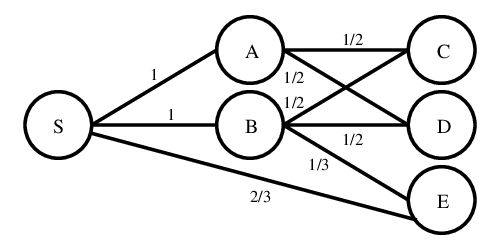
Refer to caption — Figure 1: Directed Acyclic Graph for Label Representation

Throughout this paper, we will refer to parent and child operators, $.P$ and $.C$ respectively. These reflect the direction of flow (always from parent to children) and multiplier accumulation (always from child to parents). In addition, edges in this graph, and corresponding parent/child operators can have multiplicity, that is, multiple edges can exist between two vertices indicating some rational weighting of relative parts. The parent-child operators for the graph in Figure 1 are:

\begin{array}[]{lll}S.P=\emptyset&&S.C=\{A,B,E\}\\ A.P=\{S\}&&A.C=\{C,D\}\\ B.P=\{S\}&&B.C=\{C,D,E\}\\ C.P=\{A,B\}&&C.C=\emptyset\\ D.P=\{A,B\}&&D.C=\emptyset\\ E.P=\{A,B,S\}&&E.C=\emptyset\\ \end{array}

As with the general hierarchical formulation [10], these operators have consistency requirements. That is, they must form a rooted DAG with the properties:

•

there exists only one label, $S$ , has no parent ( $S.P=\emptyset$ ),
•

the parent/child relationship is preserved ( $A\in B.P\leftrightarrow B\in A.C$ ),
•

there are no cycles (no label can be a child, grandchild, great-grandchild, etc… of itself) and that the graph is connected. Note that if this property holds for the child operator, it must also hold for the parent operator due to the above properties, and
•

the edge weights are non-negative and normalized for each child, that is $\forall L\,\sum_{L^{\prime}\in L.C}w_{(L^{\prime},L)}=1$ .

As with the Potts model [13] we would like to define the set of end-labels, $\mathbb{L}$ , as a partition of the image, that is:

\bigcup_{L\in\mathbb{L}}\Omega_{L}=\Omega\text{ and }\forall L_{1},L_{2}\in\mathbb{L}\,(L_{1}\neq L_{2}\implies L_{1}\cap L_{2}=\emptyset)\text{ .}

(1)

Unlike those in the Ishikawa [7] model and generalized hierarchical max-flow model [10], the intermediate labels do not immediately lend themselves to a set-theoretic interpretation since they are not constrained to be the union of end-labels. (Although, this case will be explicitly explored in Section 6 with corresponding DAG structure.) Nevertheless, the labeling function, $u_{L}(x)\in[0,1]$ has the following properties:[6, 14, 15]

u_{L}(x)=\left\{\begin{array}[]{ll}1,&x\in\Omega_{L}\\ 0,&x\not\in\Omega_{L}\\ \end{array}\right.

(2)

\int_{\delta\Omega_{L}}S_{L}(x)dx=\int_{\Omega}S_{L}(x)|\nabla u_{L}(x)|dx

(3)

for labels in $\mathbb{L}$ . In the case where the DAG forms a hierarchy, the same constraints apply as in the generalized hierarchical model. Otherwise, the non-unit multiplicands render the union operator meaningless. In terms of labeling function, the intermediate nodes are defined as:

u_{L}(x)=\sum\limits_{L^{\prime}\in L.C}w_{(L,L^{\prime})}u_{L^{\prime}}(x)\text{ .}

(4)

These yield the convex relaxed generalized hierarchical model:

These formulations can be solved with global optimality for probabilistic labels, which will be demonstrated by this paper. However, it is only an approximation algorithm for models under integrality constraints on the end-labels, as demonstrated by the NP-hardness of the Potts model, even over finite lattices[16].

As with previous approaches, we only consider the case where the end-labels have non-zero data terms. To prove that this does not limit the applicability of the method, a similar linear-time data term pushdown proof can be constructed along the lines presented by Baxter at al.[10]

The modeling approach is derived from those presented by Yuan et al.[6, 14]] and follows the same format, using duality through an augmented Langrangian formulation. The primal model represents network flow maximization through a large graph with only the sink flows constrained. The dual of this formulation is the DAGMF equation (5) as we shall prove in this section. We can write the primal model as:

\displaystyle\underset{p,q}{\max}

\displaystyle\int_{\Omega}p_{S}(x)dx

(6)

subject to the constraints

$\displaystyle p_{L}(x)$	$\displaystyle\leq D_{L}(x),\text{ where }L.C=\emptyset$	(7)
$\displaystyle\|q_{L}(x)\|$	$\displaystyle\leq\alpha_{L}S_{L}(x)\text{ }L\neq S$
$\displaystyle 0$	$\displaystyle=\operatorname{div}q_{L}(x)+p_{L}(x)-\sum_{L^{\prime}\in L.P}w_{(L^{\prime},L)}p_{L^{\prime}}(x)\text{ .}$

This is equivalent to a multi-flow problem over a large graph constructed from the image dimensions and the provided directed acyclic graph as overall architecture. Other than constraints put on the magnitude of the spatial flows, and the capacity of the sink flows ( $p_{L}(x)$ where $L.C=\emptyset$ ), the system is assumed to have infinite capacity. This is a strict generalization of the hierarchical formed explored by Baxter et al.[10] considering hierarchies to be a specific class of rooted DAG.

The primal model can be converted to a primal-dual model through the use of Lagrangian multipliers over the flow conservation constraint $G_{L}(x)=\operatorname{div}q_{L}(x)+p_{L}(x)-\sum_{L^{\prime}\in L.P}w_{(L^{\prime},L)}p_{L^{\prime}}(x)=0$ yielding the Lagrangian:

$\displaystyle\underset{u}{\min}\underset{p,q}{\max}$	$\displaystyle\left(\int_{\Omega}p_{S}(x)dx+\sum_{\forall L\neq S}\int_{\Omega}u_{L}(x)G_{L}(x)dx\right)$	(8)
$\displaystyle p_{L}(x)$	$\displaystyle\leq D_{L}(x),\text{ where }L.C=\emptyset$
$\displaystyle\|q_{L}(x)\|$	$\displaystyle\leq\alpha_{L}S_{L}(x)\text{ }L\neq S\text{ .}$

First, we must ensure that equation (8) is convex with respect to $u$ , considering $p,q$ to be fixed, and concave with respect to $p,q$ with $u$ fixed, as to meet the requirements of the minimax theorem. [17] Considering $p,q$ as fixed, $G$ is obviously fixed as well, implying that equation (8) is linear over $u$ and therefore convex. It should also be noted that $G$ is a linear function of $p,q$ , meaning that (8) is again linear and therefore concave with respect to $p,q$ This implies the existence of a saddle point and the equivalence of the formulation regardless of the order of the prefix max and min operators under the minimax theorem. [17]

As implied in the previous section, we can find the saddle point through the optimization of the sink-flows, $p_{L}$ , working bottom-up and the spatial flows within each label. For the sake of simplicity, we refer to an ordering $\mathbb{O}$ generated by topologically sorting the graph $G=\left(\mathbb{V}\cup\{S\},\{(L_{1},L_{2})|L_{2}\in L_{1}.P\}\right)$ . We proceed through the graph in that order. Starting with any label, $L$ , such that $L.C=\emptyset$ we can isolate $p_{L}$ in (8) giving:

		$\displaystyle\underset{u_{L}}{\min}\underset{p_{L}(x)\leq D_{L}(x)}{\max}\int_{\Omega}u_{L}(x)p_{L}(x)dx$		(9)
	$\displaystyle=$	$\displaystyle\underset{u_{L}(x)\geq 0}{\min}\int_{\Omega}u_{L}(x)D_{L}(x)dx$		(9)

when $u_{L}(x)\geq 0$ . (If $u_{L}(x)<0$ , the function can be arbitrarily maximized by $p_{L}(x)\to-\infty$ .) Working through $\mathbb{O}$ , every label, $L$ , where $L.C\neq\emptyset$ and $L.P\neq\emptyset$ can be isolated in (8) as:

\underset{u}{\min}\underset{p_{L}(x)}{\max}\left(\int_{\Omega}u_{L}(x)p_{L}(x)dx-\sum_{\forall L^{\prime}\in L.C}\int_{\Omega}w_{(L,L^{\prime})}u_{L^{\prime}}(x)p_{L}(x)dx\right)=0

(10)

at the saddle point defined by $u_{L}(x)=\sum_{\forall L^{\prime}\in L.C}w_{(L,L^{\prime})}u_{L^{\prime}}(x)$ . Lastly, the source flow, $p_{S}$ , can be isolated in a similar manner, that is:

\underset{u}{\min}\underset{p_{S}(x)}{\max}\left(\int_{\Omega}p_{S}(x)dx-\sum_{\forall L^{\prime}\in S.C}\int_{\Omega}w_{(S,L^{\prime})}u_{L^{\prime}}(x)p_{S}(x)dx\right)=0

(11)

at the saddle point defined by $1=\sum_{\forall L^{\prime}\in S.C}w_{(S,L^{\prime})}u_{L^{\prime}}(x)$ . These constraints combined yield the labeling constraints in the original formulation. The maximization of the spatial flow functions can be expressed in a well-studied form [18] as:

$\displaystyle\int_{\Omega}u_{L}(x)\dvg q_{L}(x)dx$	$\displaystyle=\int_{\Omega}\left(\dvg(u_{L}(x)q_{L}(x))-q(x)\cdot\nabla u_{L}(x)\right)dx$	(12)
	$\displaystyle=\int_{\Omega}\dvg(u_{L}(x)q_{L}(x))dx-\int_{\Omega}q_{L}(x)\cdot\nabla u_{L}(x)dx$
	$\displaystyle=\oint_{\delta\Omega}u_{L}(x)q_{L}(x)\cdot d\mathbf{s}-\int_{\Omega}q_{L}(x)\cdot\nabla u_{L}(x)dx$
	$\displaystyle=-\int_{\Omega}q_{L}(x)\cdot\nabla u_{L}(x)dx$
$\displaystyle\underset{\|q_{L}\|\leq\alpha_{L}S_{L}(x)}{\max}\int_{\Omega}u_{L}(x)\dvg q_{L}(x)dx$	$\displaystyle=\underset{\|q_{L}\|\leq\alpha_{L}S_{L}(x)}{\max}-\int_{\Omega}q_{L}(x)\cdot\nabla u_{L}(x)dx$
	$\displaystyle=-\int_{\Omega}\left(-\frac{\alpha_{L}S_{L}(x)}{\|\nabla u_{L}(x)\|}\nabla u_{L}(x)\right)\cdot\nabla u_{L}(x)dx$
	$\displaystyle=\int_{\Omega}\alpha_{L}S_{L}(x)\|\nabla u_{L}(x)\|dx$
$\displaystyle\underset{u_{L}\geq 0}{\min}\underset{\|q_{L}\|\leq\alpha_{L}S_{L}(x)}{\max}\int_{\Omega}u_{L}(x)\dvg q_{L}(x)dx$	$\displaystyle=\underset{u_{L}\geq 0}{\min}\int_{\Omega}\alpha_{L}S_{L}(x)\|\nabla u_{L}(x)\|dx\text{ .}$

The above implies that we can express the saddle point of equation (8) as the original energy functional, (5), and therefore, finding the saddle point of (8) is equivalent to solving the DAGMF segmentation problem.

To address the optimization problem, we can find this saddle point by augmenting the Lagrangian function [19]:

$\displaystyle\underset{u}{\min}\underset{p,q}{\max}$	$\displaystyle\left(\int_{\Omega}p_{S}(x)dx+\sum_{\forall L\neq S}\int_{\Omega}u_{L}(x)G_{L}(x)dx-\frac{c}{2}\sum_{\forall L\neq S}\int_{\Omega}G_{L}(x)^{2}dx\right)$	(13)
$\displaystyle p_{L}(x)$	$\displaystyle\leq D_{L}(x),\text{ }\forall L(L.C=\emptyset)$
$\displaystyle\|q_{L}(x)\|$	$\displaystyle\leq\alpha_{L}S_{L}(x)\text{ }L\neq S$

where $c$ is a positive penalty parameter encouraging faster convergence to solutions that fulfill the optimization constraints. Using this formula, we can iteratively maximize each component. The solution steps are:

Maximize (13) over $q_{L}$ at each vertex by:

q_{L}(x)\leftarrow\operatorname{Proj}_{|q_{L}(x)|\leq\alpha_{L}S_{L}(x)}\left(q_{L}(x)+\tau\nabla\left(\dvg q_{L}(x)+p_{L}(x)-\sum_{L^{\prime}\in L.P}w_{(L^{\prime},L)}p_{L^{\prime}}(x)-u_{L}(x)/c\right)\right)

which is a Chambolle’s projection iteration. [20] $\tau$ is a small positive gradient descent parameter.

Maximize (13) the out-flow to the sink, $p_{L}$ where $L.C=\emptyset$ ,analytically by:

p_{L}(x)\leftarrow\min\{D_{L}(x),\sum_{L^{\prime}\in L.P}w_{(L^{\prime},L)}p_{L^{\prime}}(x)-\dvg q_{L}(x)+u_{L}(x)/c\}

Maximize (13) the flow between vertices, $p_{L}$ where $L.C\neq\emptyset$ and $L.P\neq\emptyset$ , analytically by:

	$\displaystyle p_{L}(x)\leftarrow\frac{1}{1+\sum_{L^{\prime}\ inL.C}w_{(L,L^{\prime})}^{2}}$	$\displaystyle\left(\sum_{L^{\prime}\in L.P}w_{(L^{\prime},L)}p_{L^{\prime}}(x)-\dvg q_{L}(x)+u_{L}(x)/c\right.$
		$\displaystyle\left.+\sum_{\forall L^{\prime}\in L.C}w_{(L,L^{\prime})}\left(p_{L^{\prime}}(x)+\dvg q_{L^{\prime}}(x)+\sum_{L^{\prime\prime}\in L^{\prime}.P/L}w_{(L^{\prime\prime},L^{\prime})}p_{L^{\prime\prime}}(x)-u_{L^{\prime}}(x)/c\right)\right)$

Maximize (13) over the source flow, $p_{S}$ , analytically by:

	$\displaystyle p_{S}(x)\leftarrow\frac{1}{1+\sum_{L^{\prime}\ inS.C}w_{(S,L^{\prime})}^{2}}$	$\displaystyle\left(1/c+\right.$
		$\displaystyle\left.\sum_{\forall L^{\prime}\in S.C}w_{(S,L^{\prime})}\left(p_{L^{\prime}}(x)+\dvg q_{L^{\prime}}(x)+\sum_{L^{\prime\prime}\in L^{\prime}.P/S}w_{L^{\prime\prime},L^{\prime}}p_{L^{\prime\prime}}(x)-u_{L^{\prime}}(x)/c\right)\right)$

Minimize (13) over $u_{L}$ at each vertex analytically by:

u_{L}(x)\leftarrow u_{L}(x)-c\left(\dvg q_{L}(x)-\sum_{L^{\prime}\in L.P}w_{(L^{\prime},L)}p_{L^{\prime}}(x)+p_{L}(x)\right)

Note that within each step there exists a large amount of inherent parallelism, that is, each voxel $x$ can be accounted for completely independently of all other voxels in steps 2-5, and with only a dependence on a local neighbourhood in step 1. This inherent parallelism allows for GPGPU acceleration of each step with relative ease.

To improve the convergence rate, we perform an initialization step that ensures optimality for the zero-smoothness condition. This is achieved by initializing the system with optimal flows and multipliers under the assumption that all spatial flows are zero. To ensure faster convergence, we order the tasks using a topological sort over the graph. In this ordering, each child label occurs only after all of its parents. The inverse ordering $\mathbb{O}^{-1}$ is the opposite. This is equivalent to the bottom-up approach used by Baxter et al. [10] over hierarchies. In addition, each label is equipped with two ‘working’ buffers, $\rho_{L}(x)$ and $\sigma_{L}(x)$ , for the purposes of accumulation.

Topological sort (

\mathbb{V}\cup\{S\}

\{(L_{1},L_{2})|L_{2}\in L_{1}.P\}

) into ordering

\mathbb{O}

with reverse ordering

\mathbb{O}^{-1}

;

InitializeSolution() ;

while not converged do

UpdateFlows() ;

for $\forall L$ do

\forall x,u_{L}(x)\leftarrow u_{L}(x)-c\left(\dvg q_{L}(x)-\rho_{L}(x)+p_{L}(x)\right)

;

end for

end while

which makes use of the following function definitions:

UpdateFlows()

for $\forall L\neq S$ do

\forall x,q_{L}(x)\leftarrow\operatorname{Proj}_{|q_{L}(x)|\leq S_{L}(x)}\left(q_{L}+\tau\nabla\left(\dvg q_{L}(x)+p_{L}(x)-\rho_{L}(x)-u_{L}(x)/c\right)\right)

;

end for

Clear

\rho_{L}(x)

for all labels ;

for each $L$ in order $\mathbb{O}$ do

for each $L^{\prime}\in L.C$ do

\forall x,\rho_{L^{\prime}}(x)\leftarrow\rho_{L^{\prime}}(x)+w_{(L,L^{\prime})}p_{L}(x)

;

end for

if $L.C\neq\emptyset$ and $L.P\neq\emptyset$ then

\forall x,\sigma_{L}(x)\leftarrow\rho(x)-\dvg q_{L}(x)+u_{L}(x)/c

;

else if $L=S$ then

\forall x,\sigma_{S}(x)\leftarrow 1/c

;

end if

end for

for each $L$ in order $\mathbb{O}^{-1}$ do

if $L.C=\emptyset$ then

\forall x,p_{L}(x)\leftarrow\min\{D_{L}(x),\rho_{L}(x)-\dvg q_{L}(x)+u_{L}(x)/c\}

;

for $L^{\prime}\in L.P$ do

\forall x,\sigma_{L^{\prime}}(x)\leftarrow\sigma_{L^{\prime}}(x)+w_{(L^{\prime},L)}\left(\dvg q_{L^{\prime}}(x)+p_{L^{\prime}}(x)-\rho_{L^{\prime}}(x)+w_{L^{\prime},L}p_{L}(x)\right)

;

end for

else if $L=S$ then

\forall x,p_{S}(x)\leftarrow\frac{1}{\sum_{L^{\prime}\in S.C}w_{(S,L^{\prime})}^{2}}\sigma_{S}(x)

;

else

\forall x,p_{L}(x)\leftarrow\frac{1}{1+\sum_{L^{\prime}\in L.C}w_{(L,L^{\prime})}^{2}}\sigma_{L}(x)

;

for $L^{\prime}\in L.P$ do

\forall x,\sigma_{L^{\prime}}(x)\leftarrow\sigma_{L^{\prime}}(x)+w_{(L^{\prime},L)}\left(\dvg q_{L^{\prime}}(x)+p_{L^{\prime}}(x)-\rho_{L^{\prime}}(x)+w_{L^{\prime},L}p_{L}(x)\right)

;

end for

end if

end for

InitializeSolution()

Clear

u_{L}(x),q_{L}(x)

for all labels;

for each $L$ in order $\mathbb{O}^{-1}$ do

\forall x,p_{L}(x)\leftarrow\underset{L^{\prime}.C=\emptyset}{\min}D_{L^{\prime}}(x)

;

\forall x,\rho_{L}(x)\leftarrow\underset{L^{\prime}.C=\emptyset}{\min}D_{L^{\prime}}(x)

;

if $L.C=\emptyset$ then

if $L\in\underset{L^{\prime}.C=\emptyset}{\argmin}D_{L^{\prime}}(x)$ then

\forall x,u_{L}(x)\leftarrow 1/|\underset{L^{\prime}.C=\emptyset}{\argmin}D_{L^{\prime}}(x)|

;

else

\forall x,u_{L}(x)\leftarrow 0

;

end if

for each $L^{\prime}\in L.P/\{S\}$ do

\forall x,u_{L^{\prime}}(x)\leftarrow u_{L^{\prime}}(x)+w_{(L^{\prime},L)}u_{L}(x)

;

end for

For the sake of conciseness, the ‘for $\forall x$ do ’ loops surrounding each assignment operation have been replaced with the prefix $\forall x$ in both the algorithm and the function definitions.

As demonstrated in the introduction, continuous max-flow segmentation models have been progressing towards more and more general regularization structures. In terms of a discrete analogue, the most general structure possible would be:

\displaystyle\underset{\{\Omega_{L}\}}{\min}\text{ }E=\sum\limits_{\forall L}\left(\int_{\Omega_{L}}D_{L}(x)dx+\int_{\delta\Omega_{L}}S_{L}(x)dx\right)

(14)

in which $L$ could refer to either an end-label in $\mathbb{L}$ or a subset $H\subset\mathbb{L}$ with $\Omega_{L}=\bigcup_{L^{\prime}\in H}\Omega_{L^{\prime}}$ . We refer to this problem as having arbitrary super-object regularization in that it incorporates all possible regularization while maintaining the discrete analogue for intermediate labels. It is easy to see it as a generalization of Potts[13], Ishikawa[7], and General Hierarchical[10] models. This section aims to illustrate this as a subclass of that represented by DAGMF.

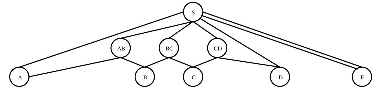
To show how arbitrary super-object regularization can be implemented with DAGMF, we must consider the construction of a DAG with associated transformations on smoothness parameters. First, let us add a vertex to the graph for the source node, $S$ , and one for each end-label in $\mathbb{L}$ . To do so, let us consider $\mathbb{G}\subset 2^{\mathbb{L}}$ to be the set of super-objects represented in the problem, not including end-labels. We will associate a vertex in the DAG to each element, $G$ , in this set. Each of these vertices has $S$ as their sole parent, and their only children will be vertices corresponding to the end-labels in $G$ . Lastly, we must ensure that all end-label vertices have the same number of parents, so we can add edges between $S$ and each vertex (allowing multiplicity) until they do. (Note that each end-label will have $r\leq|\mathbb{G}|$ parents.) An example of this is given in Figure 2.

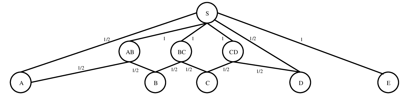
Before the algorithm can be used, we must determine edge weights and eliminate multiplicities in the edges. We do this by associated the unnormalized edge weight with the multiplicity of the edge, followed by a normalization step to ensure the weights are valid. The corresponding example is given in Figure 3.

Returning to the general case, if we consider the equation associated with this graph, we will find it is:

which is equivalent to the following by multiplying the labelling functions for $G\in\mathbb{G}$ by $r$

This indicates that the intended regularization field for $G\in\mathbb{G}$ must be multiplied by $r$ for correct scaling, and for the union operator to be a discrete analogue for addition (since the multiplicand is removed in the constraint equations).

In this paper, we present an algorithm for addressing max-flow segmentation problems where the underlying architecture is a directed acyclic graph. Using this architecture, we can achieve arbitrary super-object regularization, making it more general version of Generalized Hierarchical Max-Flow[10] and thus both Potts and Ishikawa models. Such a regularization mechanism allows for the definition of more flexible part/whole relationships, where any individual part could belong to more than one whole, a capability not present in any earlier extendable model. These also represent the most general form of ordering relationships possible while maintaining an analogous purely discrete problem.

This solver has been implemented using the NVIDIA Compute Unified Device Architecture (CUDA) taking advantage of the inherent parallelism within each optimization step. Additional concurrency between steps has been exploited to improve computational speed and allow for multiple graphics cards to be used simultaneously on a single segmentation problem.

The authors would like to acknowledge Dr. Elvis Chen, Kamyar Abhari, and Jonathan McLeod for their invaluable discussion, editing, and technical support.

$\displaystyle\underset{u}{\text{minimize}}$

$\displaystyle E(u)=\sum\limits_{\forall L}\int_{\Omega}\left(D_{L}(x)u_{L}(x)+S_{L}(x)|\nabla u_{L}(x)|\right)dx$

$\displaystyle\text{subject to}$

$\displaystyle\forall L(u_{L}(x)\geq 0)$

$\displaystyle\forall L\left(u_{L}(x)=\sum\limits_{L^{\prime}\in L.C}w_{(L,L^{\prime})}u_{L^{\prime}}(x)\right)$

$\displaystyle u_{S}(x)=1\text{ .}$

[1] Y. Y. Boykov and M.-P. Jolly, “Interactive graph cuts for optimal boundary & region segmentation of objects in ND images,” in Computer Vision, 2001. ICCV 2001. Proceedings. Eighth IEEE International Conference on, 1, pp. 105––112, 2001.
[2] Y. Boykov, O. Veksler, and R. Zabih, “Fast approximate energy minimization via graph cuts,” IEEE Transactions on Pattern Analysis and Machine Intelligence 23(11), pp. 1222–1239, 2001.
[3] Y. Boykov and V. Kolmogorov, “An experimental comparison of min-cut/max-flow algorithms for energy minimization in vision,” Pattern Analysis and Machine Intelligence, IEEE Transactions on 26(9), pp. 1124––1137, 2004.
[4] Y. Boykov, O. Veksler, and R. Zabih, “Markov random fields with efficient approximations,” in Computer vision and pattern recognition, 1998. Proceedings. 1998 IEEE computer society conference on, pp. 648––655, 1998.
[5] S. Z. Li, Markov Random Field Modeling in Image Analysis, Springer, Jan. 2009.
[6] J. Yuan, E. Bae, and X.-C. Tai, “A study on continuous max-flow and min-cut approaches,” in Computer Vision and Pattern Recognition (CVPR), 2010 IEEE Conference on, pp. 2217––2224, 2010.
[7] H. Ishikawa, “Exact optimization for markov random fields with convex priors,” IEEE Transactions on Pattern Analysis and Machine Intelligence 25(10), pp. 1333–1336, 2003.
[8] E. Bae, J. Yuan, X.-C. Tai, and Y. Boykov, “A fast continuous max-flow approach to non-convex multi–labeling problems,” 2011.
[9] A. Delong and Y. Boykov, “Globally optimal segmentation of multi-region objects,” in Computer Vision, 2009 IEEE 12th International Conference on, pp. 285–292, IEEE, 2009.
[10] J. S. Baxter, M. Rajchl, J. Yuan, and T. M. Peters, “A continuous max-flow approach to general hierarchical multi-labelling problems,” arXiv preprint arXiv:1404.0336 , 2014.
[11] M. Rajchl, J. Yuan, J. White, E. Ukwatta, J. Stirrat, C. Nambakhsh, F. Li, and T. Peters, “Interactive hierarchical max-flow segmentation of scar tissue from late-enhancement cardiac MR images,” IEEE Transactions on Medical Imaging , 2014.
[12] J. Yuan, W. Qiu, E. Ukwatta, M. Rajchl, Y. Sun, and A. Fenster, “An efficient convex optimization approach to 3D prostate MRI segmentation with generic star shape prior,” Prostate MR Image Segmentation Challenge, MICCAI , 2012.
[13] R. B. Potts, “Some generalized order-disorder transformations,” in Proceedings of the Cambridge Philosophical Society, 48, pp. 106––109, 1952.
[14] J. Yuan, E. Bae, X.-C. Tai, and Y. Boykov, “A continuous max-flow approach to potts model,” in Computer Vision – ECCV 2010, K. Daniilidis, P. Maragos, and N. Paragios, eds., Lecture Notes in Computer Science, pp. 379–392, Springer Berlin Heidelberg, Jan. 2010.
[15] E. Bae, J. Yuan, and X.-C. Tai, “Global minimization for continuous multiphase partitioning problems using a dual approach,” International journal of computer vision 92(1), pp. 112––129, 2011.
[16] V. Kolmogorov and R. Zabih, “Computing visual correspondence with occlusions using graph cuts,” in Computer Vision, 2001. ICCV 2001. Proceedings. Eighth IEEE International Conference on, 2, pp. 508––515, 2001.
[17] I. Ekeland and R. Temam, “Convex analysis and variational problems,” 1976.
[18] E. Giusti, Minimal surfaces and functions of bounded variation, vol. 80, Birkhauser, 1984.
[19] D. P. Bertsekas, “Nonlinear programming,” 1999.
[20] A. Chambolle, “An algorithm for total variation minimization and applications,” Journal of Mathematical imaging and vision 20(1-2), pp. 89––97, 2004.