跳到论文正文
W Papers独立论文阅读器 arXiv:1405.0891 论文正文 计算阅读时间 · 0%
引用这篇论文根据当前论文元数据生成,正式投稿前建议核对。


License: arXiv.org perpetual non-exclusive license
arXiv:1405.0891v1 [cs.IT] 05 May 2014

Unequal Message Protection: Asymptotic and Non-Asymptotic Tradeoffs

Yanina Y. Shkel, Student Member, IEEE ††thanks: This paper was presented in part at the International Symposium on Information Theory, Istanbul, Turkey, July 2013. Affiliation: Department of Electrical and Computer Engineering, University of Wisconsin - Madison    Vincent Y. F. Tan, Member, IEEE Affiliation: Department of Electrical and Computer Engineering, National University of Singapore    Stark C. Draper, Member, IEEE Affiliation: Department of Electrical and Computer Engineering, University of Toronto
Abstract

We study a form of unequal error protection that we term “unequal message protection” (UMP). The message set of a UMP code is a union of mm disjoint message classes. Each class has its own error protection requirement, with some classes needing better error protection than others. We analyze the tradeoff between rates of message classes and the levels of error protection of these codes. We demonstrate that there is a clear performance loss compared to homogeneous (classical) codes with equivalent parameters. This is in sharp contrast to previous literature that considers UMP codes. To obtain our results we generalize finite block length achievability and converse bounds due to Polyanskiy-Poor-Verdú. We evaluate our bounds for the binary symmetric and binary erasure channels, and analyze the asymptotic characteristic of the bounds in the fixed error and moderate deviations regimes. In addition, we consider two questions related to the practical construction of UMP codes. First, we study a “header” construction that prefixes the message class into a header followed by data protection using a standard homogeneous code. We show that, in general, this construction is not optimal at finite block lengths. We further demonstrate that our main UMP achievability bound can be obtained using coset codes, which suggests a path to implementation of tractable UMP codes.

I Introduction

We consider a channel coding problem of communicating a random message ww, selected from a set of messages ℳ\mathcal{M}, over a noisy channel WW. Our problem is different from the classical channel coding set up in the following ways. First, we dispense with the usual assumption that messages in ℳ\mathcal{M} are equiprobable. Second, we consider unequal error protection (UEP), that is, some information is provided better error guarantees than other. Our main object of study is message-wise UEP codes which we term “unequal message protection” (UMP) codes. The message set of a UMP code is a union of mm disjoint message classes, ℳ={ℳi}i=1m\mathcal{M}=\{\mathcal{M}_{i}\}_{i=1}^{m}. Each class has its own error protection requirement, with some classes needing better error protection than others. We assume that messages within the same class are equally likely to be selected for transmission, but messages from different message classes could have different probabilities of selection. In this way, UMP codes are well suited for modeling a non-uniform prior on the message set as well as unequal error protection.

Formally, a general channel from 𝖠\mathsf{A} to 𝖡\mathsf{B} is a stochastic kernel W⁡(b|a)W(b|a) satisfying ∑b∈𝖡W⁡(b|a)=1\sum_{b\in\mathsf{B}}W(b|a)=1 for all a∈𝖠a\in\mathsf{A}. Consider the following one-shot definition of a UMP code. In other words, the channel WW is only used once.

Definition 1 (UMP code).

An ((Mi)i=1m,(ϵi)i=1m)\left((M_{i})_{i=1}^{m},(\epsilon_{i})_{i=1}^{m}\right)-UMP code for WW is a tuple ({ℳi}i=1m,𝖿,𝗀)\left(\{\mathcal{M}_{i}\}_{i=1}^{m},\mathsf{f},\mathsf{g}\right) consisting of

  1. 1.

    mm disjoint message classes {ℳ1,…,ℳm}\{\mathcal{M}_{1},\ldots,\mathcal{M}_{m}\} forming the message set ℳ:=∪i=1mℳi\mathcal{M}:=\cup_{i=1}^{m}\mathcal{M}_{i} and satisfying |ℳi|=Mi|\mathcal{M}_{i}|=M_{i} for each i∈{1,2,…​m}i\in\{1,2,\dots m\}

  2. 2.

    An encoder 𝖿:ℳ→𝖠\mathsf{f}:\mathcal{M}\to\mathsf{A}

  3. 3.

    A decoder 𝗀:𝖡→ℳ\mathsf{g}:\mathsf{B}\to\mathcal{M}

such that for all i∈{1,2,…​m}i\in\{1,2,\dots m\}, the average error probabilities for each message class satisfy

1Mi​∑w∈ℳiW⁡(𝖡∖𝗀−1​(w)|𝖿⁡(w))≤ϵi.\frac{1}{M_{i}}\sum_{w\in\mathcal{M}_{i}}W(\mathsf{B}\setminus\mathsf{g}^{-1}(w)|\mathsf{f}(w))\leq\epsilon_{i}. (1)

If the maximum probability of error for each class also satisfies

maxw∈ℳi⁡W⁡(𝖡∖𝗀−1​(w)|𝖿⁡(w))≤ϵi\max_{w\in\mathcal{M}_{i}}W(\mathsf{B}\setminus\mathsf{g}^{-1}(w)|\mathsf{f}(w))\leq\epsilon_{i} (2)

we refer to the code as an ((Mi)i=1m,(ϵi)i=1m)\left((M_{i})_{i=1}^{m},(\epsilon_{i})_{i=1}^{m}\right)-UMP code (maximum probability of error).

We call a code with one class of codewords (m=1m=1) a ‘homogeneous code’; this corresponds to the traditional channel coding framework. Paralleling [1, 2], a homogeneous code with MM codewords and average (resp. maximum) error probability ϵ\epsilon will be referred to as an (M,ϵ)(M,\epsilon)-homogeneous code (average probability of error) (resp. (maximum probability of error)).

To motivate the present problem we note that it is related to a number of classical problems. First, the maximum vs. average error paradigm for homogeneous codes is intimately connected to UMP codes. In channel coding with an average probability of error criterion we are concerned with one error constraint: this is immediately captured by UMP codes with one class. In channel coding with a maximum probability of error criterion we are concerned with MM error constraints: the error probability of each codeword. The UMP set up is a generalization of the two since it allows for error constraint of arbitrary groupings of messages. Formally, we state the following proposition.

Proposition 1.

There exists an (M,ϵ)(M,\epsilon)-homogeneous code (average probability of error) for WW if and only if there exists an ((Mi)i=1m,(ϵi)i=1m)\left((M_{i})_{i=1}^{m},(\epsilon_{i})_{i=1}^{m}\right)-UMP code for WW such that m≥1m\geq 1, Mi≥MM_{i}\geq M and ϵi≤ϵ\epsilon_{i}\leq\epsilon for some i∈{1,2,…,m}i\in\{1,2,\dots,m\}. Likewise, there exists an (M,ϵ)(M,\epsilon)-homogeneous code (maximum probability of error) for WW if and only if there exists an ((Mi)i=1m,(ϵi)i=1m)\left((M_{i})_{i=1}^{m},(\epsilon_{i})_{i=1}^{m}\right)-UMP code for WW such that m≥Mm\geq M, Mi≥1M_{i}\geq 1 and ϵi≤ϵ\epsilon_{i}\leq\epsilon for all i∈{1,2,…,m}i\in\{1,2,\dots,m\}.

Proof.

Both assertions follow directly from Definition 1. ∎

Thus, UMP codes simultaneously capture classical channel coding with an average error probability constraint and classical channel coding with the maximum probability of error constraint, as well as a whole spectrum in between.11 1 One may note after reading Proposition 1 that the notion of an ((Mi)i=1m,(ϵi)i=1m)\left((M_{i})_{i=1}^{m},(\epsilon_{i})_{i=1}^{m}\right)-UMP code (maximum probability of error), see (2), is superfluous. The same object could be represented by a UMP code with ∑i=1mMi\sum_{i=1}^{m}M_{i} message classes, containing one codeword in each class, and having MiM_{i} classes with average error probabilities ϵi\epsilon_{i}. Nevertheless, we keep the notion of a UMP code with maximum probability of error since it is conceptually and notationally convenient to do so. In light of this observation studying fundamental limits of UMP setting is interesting from a purely theoretical perspective.

Secondly, UMP codes can be connected to the problem of lossless joint source-channel coding by imposing a prior distribution on the message set ℳ\mathcal{M}. In fact, message-wise UEP has appeared explicitly or implicitly in a number of works on joint source-channel coding [3, 4, 5, 6, 7]. The main distinction between the present problem and joint source-channel coding is that in the present setting the goal is to have error guarantees for all mm classes simultaneously, whereas in joint source-channel coding only the expected error over the whole code is studied. Finally, we should mention that special classes of UMP codes have been used in streaming communication [8, 9, 10, 11]. We will discuss this application of UMP codes in some greater detail in Section VI.

The rest of this paper is structured as follows. For the remainder of this section we present additional definitions and discussion concerning UMP codes, as well as introduce information theoretic quantities used throughout the paper. In Section II we review prior work and outline the main contribution of this paper. In Section III we prove our finite block length achievability and converse bounds. In Section IV we evaluate these bounds for the binary symmetric and binary erasure channels. We also present a construction based on coset codes and numerically compare the performance of our UMP bounds to the header construction that prefixes the message class into a header followed by data protection using a standard homogeneous code. In Section V we present an asymptotic analysis of UMP codes in the fixed error and moderate deviations regimes. We end with concluding remarks in Section VI.

I-A Additional Definitions and Notation

When we use the term ‘UMP code’ we refer to the triple ({ℳi}i=1m,𝖿,𝗀)\left(\{\mathcal{M}_{i}\}_{i=1}^{m},\mathsf{f},\mathsf{g}\right). It may be convenient also to refer to a UMP codebook which is the collection of particular codewords associated with ({ℳi}i=1m,𝖿,𝗀)\left(\{\mathcal{M}_{i}\}_{i=1}^{m},\mathsf{f},\mathsf{g}\right). We denote the UMP codebook by 𝒞=⋃w∈ℳ{𝖿⁡(w)}\mathcal{C}=\bigcup_{w\in\mathcal{M}}\{\mathsf{f}(w)\}. The UMP codebook is a union of subcodebooks associated with each message class. That is, 𝒞=⋃𝒞i\mathcal{C}=\bigcup\mathcal{C}_{i} where 𝒞i=⋃w∈ℳi{𝖿⁡(w)}\mathcal{C}_{i}=\bigcup_{w\in\mathcal{M}_{i}}\{\mathsf{f}(w)\}.

We may be interested in additional performance metrics for UMP codes. For example, we could study the overall error of the code in addition to the errors associated with each class. This is captured by notion of expected error.

Definition 2 (Expected Error).

The expected error of an ((Mi)i=1m,(ϵi)i=1m)\left((M_{i})_{i=1}^{m},(\epsilon_{i})_{i=1}^{m}\right)-UMP code induced by probability vector 𝛍=(μ1,…,μm){\bm{\mu}}=(\mu_{1},\dots,\mu_{m}) is

ϵ⁡(𝝁)=∑i=1mμi​ϵi.\displaystyle\epsilon({\bm{\mu}})=\sum_{i=1}^{m}\mu_{i}\epsilon_{i}. (3)

We also note that the achievability bounds presented in this paper are generalizations of homogeneous bounds developed for the maximum probability of error criterion. Proposition 1 suggest why adopting some achievability techniques that work for the average, but not the maximum, probability of error paradigm is challenging. If such adaptation were possible then we could derive a homogeneous bound with maximum probability of error criterion. However, we could still adopt bounds for average probability of error paradigm to bound the expected error of the code. We will take this approach in Theorems 5 and 6 of Section III.

If WnW^{n} is a sequence of channels indexed by nn (for example, WnW^{n} is a DMC), we may be interested in the normalized entropy of the message set assuming that the probability of selecting a message in class ii is μi\mu_{i}. We refer to this quantity as the expected rate.

Definition 3 (Expected Rate).

The expected rate of an ((Mi)i=1m,(ϵi)i=1m)\left((M_{i})_{i=1}^{m},(\epsilon_{i})_{i=1}^{m}\right)-UMP code over channel WnW^{n} induced by probability vector 𝛍=(μ1,…,μm){\bm{\mu}}=(\mu_{1},\dots,\mu_{m}) is

R⁡(𝝁)=1n​∑i=1mμi​(log⁡Mi−log⁡μi)\displaystyle R({\bm{\mu}})=\frac{1}{n}\sum_{i=1}^{m}\mu_{i}\left(\log M_{i}-\log\mu_{i}\right) (4)

bits per channel use.

Throughout this paper ii will always denote the index of a class in a UMP code, mm the number of classes, and nn the channel block length. When we study asymptotic bounds for UMP codes we will consider the situation in which the number of classes scales in block length. We will denote this scaling by mnm_{n}.

When we present the single-shot finite block length bounds for UMP codes in Section III there is no scaling in mm and so we use the notation of ((Mi)i=1m,(ϵi)i=1m)\left((M_{i})_{i=1}^{m},(\epsilon_{i})_{i=1}^{m}\right)-UMP codes. For fixed error asymptotic analysis we use ((Mn,i)i=1mn,(ϵi)i=1mn)\left((M_{n,i})_{i=1}^{m_{n}},(\epsilon_{i})_{i=1}^{m_{n}}\right)-UMP codes. We emphasize that the error probabilities are fixed, while the number of message classes is allowed to scale in nn. For moderate deviations asymptotic analysis we let rate and error probability scale with block length and use the notation ((Mn,i)i=1mn,(ϵn,i)i=1mn)\left((M_{n,i})_{i=1}^{m_{n}},(\epsilon_{n,i})_{i=1}^{m_{n}}\right)-UMP codes. Again, this is to emphasize that error probabilities, number of message classes, and messages class sizes, scale with nn.

We will use sans-serif letters to indicate alphabets in single shot setting; for example, 𝖠\mathsf{A} will usually denote the input alphabet, and 𝖡\mathsf{B} will denote the output alphabet for the channel WW. When we apply the single-shot bounds to DMCs with transition matrix WW and input/output alphabets 𝒜\mathcal{A}, ℬ\mathcal{B} we will apply them to the channel WnW^{n} and take 𝖠=𝒜n\mathsf{A}=\mathcal{A}^{n}, 𝖡=ℬn\mathsf{B}=\mathcal{B}^{n}. Calligraphic letters will denote sets and we will use 𝟙​{𝒮}\mathds{1}\left\{\mathcal{S}\right\} to denote the indicator function on some set 𝒮\mathcal{S}. Finally, we define output distributions P​WPW as P​W​(y)=∑xP⁡(x)​W​(y|x)PW(y)=\sum_{x}P(x)W(y|x) and Wx​(y)=W​(y|x)W_{x}(y)=W(y|x).

I-B Information Theoretic Quantities

To state our bounds we define the information density of (X,Y)(X,Y) with joint distribution PX​YP_{XY} as

ıX;Y​(x,y):=log⁡d​PY|X=xd​PY​(y).\displaystyle\imath_{X;Y}(x;y):=\log\frac{\mathrm{d}P_{Y|X=x}}{\mathrm{d}P_{Y}}(y). (5)

We also define two functions that relate to hypothesis testing. Consider a random variable YY defined on 𝖡\mathsf{B} that can take probability measure PP or QQ. A randomized test between these two distributions is defined by a random transformation PZ|B:𝖡→{0,1}P_{Z|B}:\mathsf{B}\to\{0,1\} where 00 indicates that the test chooses QQ. The best false alarm achievable among all randomized test with detection probability at least α\alpha is given by

βα(P,Q):=infPZ|Y:∑b∈𝖡PZ|Y​(1|b)​P​(b)≥α∑b∈𝖡PZ|Y(1|b)Q(b),\displaystyle\beta_{\alpha}(P,Q):=\inf_{P_{Z|Y}:\sum_{b\in\mathsf{B}}P_{Z|Y}(1|b)P(b)\geq\alpha}\sum_{b\in\mathsf{B}}P_{Z|Y}(1|b)Q(b), (6)

where the minimizer PZ|Y∗P_{Z|Y}^{*} is guaranteed to be attained by the Neyman-Pearson lemma, see for example [1, Appendix B].

In addition, we define a related measure of performance for the composite hypothesis test between QQ and a collection {PY|X=x}x∈𝖥\{P_{Y|X=x}\}_{x\in\mathsf{F}}

κτ(𝖥,Q):=infPZ|Y:infx∈𝖥PZ|Y​(1|x)≥τ∑b∈𝖡QY(b)PZ|Y(1|b)\displaystyle\kappa_{\tau}(\mathsf{F},Q):=\inf_{P_{Z|Y}:\inf_{x\in\mathsf{F}}P_{Z|Y}(1|x)\geq\tau}\sum_{b\in\mathsf{B}}Q_{Y}(b)P_{Z|Y}(1|b) (7)

For our asymptotic analysis we introduce the following information theoretic quantities. Denote by 𝒫\mathcal{P} the (|𝒜|−1)(|\mathcal{A}|-1)-dimensional simplex over ℝ|𝒜|\mathbb{R}^{|\mathcal{A}|} of input probability distributions. For any fixed P∈𝒫P\in\mathcal{P} define:

  • •

    mutual information as

    I⁡(P,W)=𝔼⁡[ıX;Y​(X,Y)]=∑x∈𝒜,y∈ℬP⁡(x)​W​(y|x)​log⁡W⁡(y|x)P​W​(y)\displaystyle I(P,W)=\mathbb{E}[\imath_{X;Y}(X;Y)]=\sum_{x\in\mathcal{A},y\in\mathcal{B}}P(x)W(y|x)\log\frac{W(y|x)}{PW(y)} (8)
  • •

    conditional information variance as

    V(P,W)=𝔼[𝕍ar(ıX;Y(X;Y)|X)]=∑x∈𝒜P(x)∑y∈ℬ(logW⁡(y|x)P​W​(y)−D(W(⋅|x)∥PW))2,\displaystyle V(P,W)=\mathbb{E}[\mathbb{V}ar(\imath_{X;Y}(X;Y)|X)]=\sum_{x\in\mathcal{A}}P(x)\sum_{y\in\mathcal{B}}\left(\log\frac{W(y|x)}{PW(y)}-D(W(\cdot|x)\|PW)\right)^{2}, (9)
  • •

    the channel capacity as

    C=maxP∈𝒫⁡I⁡(P,W),\displaystyle C=\max_{P\in\mathcal{P}}I(P,W), (10)
  • •

    subset of capacity achieving distributions as

    Π={P∈𝒫:I⁡(P,W)=C},\displaystyle\Pi=\left\{P\in\mathcal{P}:I(P,W)=C\right\}, (11)
  • •

    maximal and minimal conditional variance as

    Vmax\displaystyle V_{\max} =maxP∈Π⁡V⁡(P,W)\displaystyle=\max_{P\in\Pi}V(P,W) (12)
    Vmin\displaystyle V_{\min} =minP∈Π⁡V⁡(P,W)\displaystyle=\min_{P\in\Pi}V(P,W) (13)
  • •

    and the ϵ\epsilon-dispersion as

    Vϵ={Vmin,ϵ<1/2Vmax,ϵ≥1/2\displaystyle V_{\epsilon}=\left\{\begin{array}[]{cc}V_{\min},&\epsilon<1/2\\ V_{\max},&\epsilon\geq 1/2\end{array}\right.
  • •

    and finally information spectrum divergence as

    Dsϵ(P∥Q):=max{R∈ℝ:P({x:logP⁡(x)Q⁡(x)≤R})≤ϵ}.\displaystyle D_{s}^{\epsilon}(P\|Q):=\max\bigg\{R\in\mathbb{R}:P\Big(\Big\{x:\log\frac{P(x)}{Q(x)}\leq R\Big\}\Big)\leq\epsilon\bigg\}. (16)

II Problem Overview

II-A Prior Work

Prior work on message-wise UEP has been limited to the asymptotic setting and to discrete memoryless channels (DMC). The first study was by Csiszár [3] who showed that if codewords in message class ii are generated at rate RiR_{i}, then each class of codewords can have a reliability function E⁡(Ri)E(R_{i}), where E⁡(R)E(R) is the reliability function for a homogeneous (m=1m=1) codebook of rate RR.22 2 Provided the number message classes scales sub exponentially in channel block length nn A similar result, that there is no apparent performance loss from several message classes being packed into the same UMP codebook, was later obtained as part of the study of error exponents for UEP schemes by Borade-Nakiboğlu-Zheng [12].

The focus of this paper is on fixed error and moderate deviations asymptotic analyses, rather than analyses of large deviations setting, is in [3, 12]. First, consider fixing an error probability requirement for each class and study how fast corresponding rates can grow in nn. This question has received a lot of attention in recent literature for the homogeneous case. Let M∗​(ϵ,W)M^{\ast}(\epsilon,W) be the largest possible homogeneous code that attains error probability ϵ\epsilon over an arbitrary single-shot channel WW(cf. [2, Definition 2]). Strassen [13], showed that for positive dispersion DMC WW the following holds

log⁡M∗​(ϵ,Wn)=n​C−n​Vϵ​Q−1​(ϵ)+θ⁡(n)\displaystyle\log M^{\ast}(\epsilon,W^{n})=nC-\sqrt{nV_{\epsilon}}Q^{-1}(\epsilon)+\theta(n) (17)

where Q⁡(⋅)Q(\cdot) is the tail probability of a standard normal distribution and θ⁡(n)=O⁡(log⁡n)\theta(n)=O(\log n). Since then a number of works [1, 2, 14, 15] have obtained sharper bounds on the remainder term θ⁡(n)\theta(n), of which we will make use in this paper.

Recently, Wang-Ingber-Kochman [4] derived similar fixed-error asymptotic results for the message-wise UEP problem studied here. They demonstrated that the ϵ\epsilon-dispersion of each class of codewords in a codebook with mnm_{n} message classes matches the ϵ\epsilon-dispersion of each class individually, provided mnm_{n} grows at most as fast as a polynomial in block length nn. Using the notation of our paper, their result states that there is a sequence of ((Mn,i)i=1mn,(ϵi)i=1mn)\left((M_{n,i})_{i=1}^{m_{n}},(\epsilon_{i})_{i=1}^{m_{n}}\right)-UMP codes satisfying,

log⁡Mn,i=n​C−n​Vϵ​Q−1​(ϵi)+θi​(n).\displaystyle\log M_{n,i}=nC-\sqrt{nV_{\epsilon}}Q^{-1}(\epsilon_{i})+\theta_{i}(n). (18)

where θi​(n)=O⁡(log⁡n)\theta_{i}(n)=O(\log n). Just like the study of error exponents in [3, 12] this setting together with the assumption of polynomial (or smaller) scaling of mnm_{n} does not expose any tradeoffs between different classes of a UMP code.

In the asymptotic analysis presented in [13, 2, 14, 15, 4] the tolerated probability of error is fixed and the gap to capacity drops as 1n\frac{1}{\sqrt{n}}. Another natural question to ask is what happens if the rate of a code approaches capacity, but at a slower rate than in (17). This moderate deviations behavior was studied for m=1m=1 by Altuğ and Wagner in [16] for DMCs with Vmin>0V_{\min}>0 and strictly positive entries. The positive entry assumption was later relaxed by Altuğ-Wagner in [17], and by Polyanksiy-Verdú in [18]. Polyanksiy and Verdú also addressed the zero dispersion case for DMC and the additive Gaussian noise channels (AWGN). The moderate divisions results state that for positive dispersion DMC WW, and any sequence of positive real numbers (ρn)n≥1(\rho_{n})_{n\geq 1} such that

ρn→0, and ​n​ρn2→∞\displaystyle\rho_{n}\to 0,\mbox{ and }n\rho_{n}^{2}\to\infty (19)

there exists a sequence of (Mn,ϵn)(M_{n},\epsilon_{n})-homogeneous codes over WW that satisfy

log⁡Mn=n​C−n​ρn\displaystyle\log M_{n}=nC-n\rho_{n} (20)

and

lim supn→∞1n​ρn2​log⁡ϵn≤−12​V.\displaystyle\limsup_{n\to\infty}\frac{1}{n\rho^{2}_{n}}\log\epsilon_{n}\leq-\frac{1}{2V}. (21)

Conversely, for any sequence of real numbers (ρn)n=1∞(\rho_{n})_{n=1}^{\infty} satisfying (19) and any sequence of (Mn,ϵn)(M_{n},\epsilon_{n})-codes satisfying (20) it must be the case that

lim infn→∞1n​ρn2​log⁡ϵn≥−12​V.\displaystyle\liminf_{n\to\infty}\frac{1}{n\rho^{2}_{n}}\log\epsilon_{n}\geq-\frac{1}{2V}. (22)

We will call 12​V\frac{1}{2V} ‘moderate deviations exponent’ and ρn2\rho_{n}^{2} the ‘speed of convergence’. This result lies between the fixed error asymptotic analysis of [13] and the large deviations analysis [19]. To the best of the authors’ knowledge, no study of UMP codes in the moderate deviations settings has been done to date.

II-B Main Results

In this work we present a detailed analysis of UMP codes. We focus on finite block length bounds, as well as different asymptotic regimes and scaling of mnm_{n} than those considered in [3, 12, 4]. The collection of theorems presented in this work demonstrate that there is a clear performance loss in the rates of message classes and the levels of error protection compared to homogeneous codes with equivalent parameters.

To expose the tradeoffs between different classes of messages in an UMP code we begin by first deriving finite block length bounds in Section III. Our approach generalizes homogeneous achievability and converse bounds due to Polyanskiy-Poor-Verdú [2, 1]. It turns out that in the non-asymptotic regime tradeoffs are readily apparent and have a pleasing parameterization. Let M∗​(ϵ,W)M^{\ast}(\epsilon,W) be as before and define

ℒm={𝝀=(λ1,…,λm):∑i=1mλi=1,λi≥0∀i}.\displaystyle\mathcal{L}_{m}=\{{\bm{\lambda}}=(\lambda_{1},\dots,\lambda_{m}):\sum_{i=1}^{m}\lambda_{i}=1,\lambda_{i}\geq 0\quad\forall i\}. (23)

Our bounds reveal that for any 𝝀∈ℒm\bm{\lambda}\in\mathcal{L}_{m} there is a ((Mi)i=1m,(ϵi)i=1m)\left((M_{i})_{i=1}^{m},(\epsilon_{i})_{i=1}^{m}\right)-UMP code that (roughly) satisfies

Mi≤λi​M∗​(ϵi,W),i∈{1,…,m}.\displaystyle M_{i}\leq\lambda_{i}M^{\ast}(\epsilon_{i},W),\quad i\in\{1,\dots,m\}.

Conversely, every UMP code must satisfy this for some 𝝀∈ℒm\bm{\lambda}\in\mathcal{L}_{m}. Thus, this parameterization characterizes our achievability bounds (cf. Corollary 3 and Theorem 4) and our converse bounds (cf. Theorem 8).

Next, in Section V we analyze the asymptotic behavior of our bounds for DMCs, including situations in which the number of message classes scales with the channel block length. Such scalings are characterized by:

  • •

    a non-decreasing sequence mn∈ℕm_{n}\in\mathbb{N} that can scale arbitrarily in nn,

  • •

    a sequence of error probabilities (ϵi)i=1∞(\epsilon_{i})_{i=1}^{\infty} such that all error probabilities are bounded away from zero and one,

  • •

    a doubly semi-infinite two-dimensional array Λ\Lambda parametrized by nn and ii.

For any such sequence mnm_{n} we define

ℒ={Λ:(Λn,1,…,Λn,mn)∈ℒmn∀n, and Λn,i=0 if i>mn}\displaystyle\mathcal{L}=\{\Lambda:(\Lambda_{n,1},\dots,\Lambda_{n,m_{n}})\in\mathcal{L}_{m_{n}}\quad\forall n,\mbox{ and }\Lambda_{n,i}=0\mbox{ if }i>m_{n}\} (24)

where Λn,i\Lambda_{n,i} is the element of Λ\Lambda in the nnth row and iith column. This set up allows us to make the following asymptotic statement (cf. Theorem 19). Any sequence of ((Mn,i)i=1mn,(ϵi)i=1mn)\left((M_{n,i})_{i=1}^{m_{n}},(\epsilon_{i})_{i=1}^{m_{n}}\right)-UMP codes over a positive dispersion DMC WW must satisfy

log⁡Mn,i≤n​C−n​V​Q−1​(ϵi)+θi​(n)−log⁡1Λn,i\displaystyle\log M_{n,i}\leq nC-\sqrt{nV}Q^{-1}(\epsilon_{i})+\theta_{i}(n)-\log\frac{1}{\Lambda_{n,i}} (25)

for some Λ∈ℒ\Lambda\in\mathcal{L} where (similar to the m=1m=1 case), θi​(n)=O​(1)\theta_{i}(n)=O(1) if WW is singular and symmetric and θi​(n)=12​log⁡n+O⁡(1)\theta_{i}(n)=\frac{1}{2}\log n+O(1) otherwise. On the other hand, for any Λ∈ℒ\Lambda\in\mathcal{L} there is a sequence of ((Mn,i)i=1mn,(ϵi)i=1mn)\left((M_{n,i})_{i=1}^{m_{n}},(\epsilon_{i})_{i=1}^{m_{n}}\right)-UMP codes over a positive dispersion DMC WW such that

log⁡Mn,i≥n​C−n​V​Q−1​(ϵi)+θ~i​(n)−log⁡1Λn,i\displaystyle\log M_{n,i}\geq nC-\sqrt{nV}Q^{-1}(\epsilon_{i})+\tilde{\theta}_{i}(n)-\log\frac{1}{\Lambda_{n,i}} (26)

where θ~i​(n)=O​(1)\tilde{\theta}_{i}(n)=O(1). Paralleling the finite block length case the performance loss of UMP codes compared to homogeneous codes with the same error probability is captured by the set ℒ\mathcal{L}.

Finally, we analyze UMP codes in the moderate deviations regime (cf. Theorem 20). Fix Λ∈ℒ\Lambda\in\mathcal{L} and assume that a given collection of sequences ((ρn,i)n≥1)i≥1\left((\rho_{n,i})_{n\geq 1}\right)_{i\geq 1} is such that any fixed ii the sequence (ρn,i)n≥1(\rho_{n,i})_{n\geq 1} satisfies (19). Then there exists a sequence of ((Mn,i)i=1mn,(ϵn,i)i=1mn)\left((M_{n,i})_{i=1}^{m_{n}},(\epsilon_{n,i})_{i=1}^{m_{n}}\right)-UMP codes satisfying

Mn,i=⌊2n​C−n​ρn,i⌋\displaystyle M_{n,i}=\lfloor 2^{nC-n\rho_{n,i}}\rfloor (27)

and

lim supn→∞1n​(ρn,i−1n​log⁡1Λn,i)2​log⁡ϵn,i≤−12​V\displaystyle\limsup_{n\to\infty}\frac{1}{n\left(\rho_{n,i}-\frac{1}{n}\log\frac{1}{\Lambda_{n,i}}\right)^{2}}\log\epsilon_{n,i}\leq-\frac{1}{2V} (28)

for each 1≤i≤∞1\leq i\leq\infty. Conversely, any sequence of ((Mn,i)i=1mn,(ϵn,i)i=1mn)\left((M_{n,i})_{i=1}^{m_{n}},(\epsilon_{n,i})_{i=1}^{m_{n}}\right)-UMP codes satisfying (27) must satisfy

lim infn→∞1n​(ρn,i−1n​log⁡1Λn,i)2​log⁡ϵn,i≥−12​V\displaystyle\liminf_{n\to\infty}\frac{1}{n\left(\rho_{n,i}-\frac{1}{n}\log\frac{1}{\Lambda_{n,i}}\right)^{2}}\log\epsilon_{n,i}\geq-\frac{1}{2V} (29)

for some Λ∈ℒ\Lambda\in\mathcal{L}. In other words, each class of the UMP code has moderate deviations exponent 12​Vmin\frac{1}{2V_{\min}} and speed of convergence (ρn,i−1n​log⁡1Λn,i)2\left(\rho_{n,i}-\frac{1}{n}\log\frac{1}{\Lambda_{n,i}}\right)^{2}. Recall, a sequence of homogeneous codes approaching capacity at the same rate converged to the moderate deviations exponent with speed of ρn,i2\rho_{n,i}^{2}, and thus the loss in the moderate deviation setting is also captured by the set ℒ\mathcal{L}.

II-C On Construction Of Good UMP Codes

One may immediately observe that for a DMC the problem of constructing UMP codes has an immediate and asymptotically optimal (in terms of rate) solution. To encode a message from one of mm classes for transmission over a codebook of block length nn allocate the first n0n_{0} symbols to a header that encodes the class i∈{1,…,m}i\in\{1,\dots,m\} of the transmitted message. Allocate the remaining n−n0n-n_{0} symbols to transmit the message w∈ℳiw\in\mathcal{M}_{i} by using a homogeneous code. As long as mm grows sub-exponentially in nn the rate of each message class in this header-based construction can approach capacity. This is an appealing solution since it allows us to leverage existing codes as building blocks for UMP codes.

However, as shown in Section IV, the header construction is suboptimal in the finite block length regime. There is simple geometric intuition for the suboptimality. The header construction is equivalent to taking the decoding space and partitioning it into separate regions, with each region used to pack codewords from one class. The more general approach taken by our Theorems 2 and 4 is equivalent to mixing the classes throughout the whole decoding space. This allows for a more efficient packing of the codewords in the UMP codebook. See Figure 1 for an illustration of this idea. A more formal demonstration of the suboptimality is provided in Figures 2 through 5 where the header code bounds are compared to UMP coding bounds for the binary symmetric channel (BSC) and the binary erasure channel (BEC).

Refer to caption
Fig. 1: A general UMP coding construction (left) compared with a header-based construction (right). The more general construction allows for a better packing of codewords in an UMP code.

In lieu of the ‘header’ construction we demonstrate that the performance guarantees given by Corollary 3 can be achieved with a UMP code formed by taking a union of coset codes. By encoding each class with its own coset code we can construct a UMP code with good encoding complexity and decoding complexity that scales as the number of classes mm. This result is presented for the BSC and the BEC in Theorem 18.

III Finite Block Length Bounds

In this section we consider an abstract channel WWwith input/output alphabets 𝖠\mathsf{A}, 𝖡\mathsf{B} used once to transmit a message.

III-A Achievability Bounds

We begin by extending the dependence testing (DT) for maximal probability of error bound [1, Theorem 21] to UMP coding in Theorem 2. We follow [1] and present a compact version of the UMP DT bound in Corollary 3. Corollary 3 demonstrates how the resulting family of codes is parametrized by ℒm\mathcal{L}_{m}(cf. (23)). In Theorem 4 we extend the κ​β\kappa\beta-bound [1, Theorem 25] to the UMP coding case: this extension admits the parameterization by the same ℒm\mathcal{L}_{m} as Corollary 3. Finally, a consequence of Proposition 1 is that it is difficult to extend homogeneous bounds that do not work for a maximal probability of error paradigm to UMP coding. To circumvent this we make statements about the expected error of a UMP code by extending the average probability of error DT and random coding union (RCU) bounds [1, Theorems 16 & 17] in Theorem 6.

Theorem 2 (UMP Achievability Bound).

Let

  • •

    ℳ=⋃i=1mℳi\mathcal{M}=\bigcup_{i=1}^{m}\mathcal{M}_{i} be a message set with mm disjoint message classes and |ℳi|=Mi|\mathcal{M}_{i}|=M_{i},

  • •

    (PXi)i=1m(P_{X_{i}})_{i=1}^{m} be (not necessarily distinct) distributions on 𝖠\mathsf{A},

  • •

    {τi:𝖠→[0,∞]}i=1m\left\{\tau_{i}:\mathsf{A}\to[0,\infty]\right\}_{i=1}^{m} be measurable mappings,

then there exists an ((Mi)i=1m,(ϵi)i=1m)\left((M_{i})_{i=1}^{m},(\epsilon_{i})_{i=1}^{m}\right)-UMP code over the channel WW with maximum probability of error for each class not exceeding

ϵi\displaystyle\epsilon_{i} ≤ℙ[ıXi;Yi(Xi;Yi)≤logτi(Xi)]+(Mi−1)supxℙ[ıXi;Yi(x;Yi)>logτi(x)]\displaystyle\leq\mathbb{P}\left[\imath_{X_{i};Y_{i}}(X_{i};Y_{i})\leq\log\tau_{i}(X_{i})\right]+(M_{i}-1)\sup_{x}\mathbb{P}\left[\imath_{X_{i};Y_{i}}(x;Y_{i})>\log\tau_{i}(x)\right]
+∑j=1i−1Mjsupxℙ[ıXj;Yj(x;Yi)>logτj(x)]\displaystyle\quad+\sum_{j=1}^{i-1}M_{j}\sup_{x}\mathbb{P}\left[\imath_{X_{j};Y_{j}}(x;Y_{i})>\log\tau_{j}(x)\right] (30)

where PXi​Yi​(x,y)=PXi​(x)​W​(y|x)P_{X_{i}Y_{i}}(x,y)=P_{X_{i}}(x)W(y|x) (the joint distribution induced across the channel by PXiP_{X_{i}}) and PYi​(y)=PXi​W​(y)P_{Y_{i}}(y)=P_{X_{i}}W(y) (channel output distribution induced by PXiP_{X_{i}}).

In the proof, we follow the sequential random coding technique used in [1, Theorem 21]. In this way, we first construct the codebook for class 11, then for class 22, up to class mm. The main modification is for decoding rule to vary across classes: we decode to the first codeword ci,wc_{i,w} such that ıXi;Yi​(ci,w,y)>log⁡τi​(ci,w)\imath_{X_{i};Y_{i}}(c_{i,w};y)>\log\tau_{i}(c_{i,w}). See Appendix A for the proof. By letting m=1m=1 we obtain ϵ≤ℙ[ıX;Y(X;Y)≤logτ(X)]+(M−1)supxℙ[ıX;Y(x;Y)>logτ(x)]\epsilon\leq\mathbb{P}\left[\imath_{X;Y}(X;Y)\leq\log\tau(X)\right]+(M-1)\sup_{x}\mathbb{P}\left[\imath_{X;Y}(x;Y)>\log\tau(x)\right] which recovers [1, Theorem 21] exactly.

Theorem 2 presents bounds for the probability of error for each message class in an UMP code. By loosening these bounds we obtain the following parametrization by ℒm\mathcal{L}_{m}(cf. (23)).

Corollary 3 (UMP Achievability Bound - Compact Version).

Let ℳ\mathcal{M} be as in Theorem 2 and suppose that the family of input distributions (PXi)i=1m(P_{X_{i}})_{i=1}^{m} have the property that PXi​W=PXj​WP_{X_{i}}W=P_{X_{j}}W for all i,j∈{1,2,…,m}i,j\in\{1,2,\dots,m\}.33 3 This holds, for example, if (i) all mm input distributions are the same or (ii) all mm input distributions are capacity achieving. Then, for any 𝛌∈ℒm\bm{\lambda}\in\mathcal{L}_{m} there exists an ((Mi)i=1m,(ϵi)i=1m)\left((M_{i})_{i=1}^{m},(\epsilon_{i})_{i=1}^{m}\right)-UMP code with maximum probability of error for each class not exceeding

ϵi\displaystyle\epsilon_{i} ≤ℙ[ıXi;Yi(Xi;Yi)≤logMiλi]+Miλisupxℙ[ıXi;Yi(x;Yi)>logMiλi].\displaystyle\leq\mathbb{P}\left[\imath_{X_{i};Y_{i}}(X_{i};Y_{i})\leq\log\frac{M_{i}}{\lambda_{i}}\right]+\frac{M_{i}}{\lambda_{i}}\sup_{x}\mathbb{P}\left[\imath_{X_{i};Y_{i}}(x;Y_{i})>\log\frac{M_{i}}{\lambda_{i}}\right]. (31)

If the CDF of ℙ[ıXi;Yi(x;Yi)≤α]\mathbb{P}\left[\imath_{X_{i};Y_{i}}(x;Y_{i})\leq\alpha\right] does not depend on xx for any α\alpha we can restate (31) as

ϵi≤𝔼⁡[exp⁡{−[ıXi;Yi​(Xi,Yi)−log⁡Miλi]+}].\displaystyle\epsilon_{i}\leq\mathbb{E}\left[\exp\left\{-\left[\imath_{X_{i};Y_{i}}(X_{i};Y_{i})-\log\frac{M_{i}}{\lambda_{i}}\right]^{+}\right\}\right]. (32)

In (31) and  (32) the probability ad the expectation is taken with respect to PXi​Yi​(x,y)=PXi​(x)​W​(y|x)P_{X_{i}Y_{i}}(x,y)=P_{X_{i}}(x)W(y|x).

Proof.

Fix 𝝀∈ℒm\bm{\lambda}\in\mathcal{L}_{m} and define

Ai=Miλisupx∈𝖠ℙ[ıXi;Yi(x;Yi)>logτi(x)].\displaystyle A_{i}=\frac{M_{i}}{\lambda_{i}}\sup_{x\in\mathsf{A}}\mathbb{P}\left[\imath_{X_{i};Y_{i}}(x;Y_{i})>\log\tau_{i}(x)\right].

The order in which we generate sub-codebooks for different classes in Theorem 2 is arbitrary; so for a given message set, input distributions, and 𝝀∈ℒm\bm{\lambda}\in\mathcal{L}_{m} we may assume without loss of generality that A1≤A2≤⋯≤AmA_{1}\leq A_{2}\leq\dots\leq A_{m}. Observe that by loosening (30) we obtain

ϵi\displaystyle\epsilon_{i} ≤ℙ[ıXi;Yi(Xi;Yi)≤logτi(x)]+∑j=1iMjsupx∈𝖠ℙ[ıXj;Yj(x;Yi)>logτj(x)]\displaystyle\leq\mathbb{P}\left[\imath_{X_{i};Y_{i}}(X_{i};Y_{i})\leq\log\tau_{i}(x)\right]+\sum_{j=1}^{i}M_{j}\sup_{x\in\mathsf{A}}\mathbb{P}\left[\imath_{X_{j};Y_{j}}(x;Y_{i})>\log\tau_{j}(x)\right] (33)
=ℙ[ıXi;Yi(Xi;Yi)≤logτi(x)]+∑j=1iMjsupx∈𝖠ℙ[ıXj;Yj(x;Yj)>logτj(x)]\displaystyle=\mathbb{P}\left[\imath_{X_{i};Y_{i}}(X_{i};Y_{i})\leq\log\tau_{i}(x)\right]+\sum_{j=1}^{i}M_{j}\sup_{x\in\mathsf{A}}\mathbb{P}\left[\imath_{X_{j};Y_{j}}(x;Y_{j})>\log\tau_{j}(x)\right] (34)
=ℙ[ıXi;Yi(Xi;Yi)≤logτi(x)]+∑j=1iλjAj\displaystyle=\mathbb{P}\left[\imath_{X_{i};Y_{i}}(X_{i};Y_{i})\leq\log\tau_{i}(x)\right]+\sum_{j=1}^{i}\lambda_{j}A_{j} (35)
≤ℙ[ıXi;Yi(Xi;Yi)≤logτi(x)]+Ai\displaystyle\leq\mathbb{P}\left[\imath_{X_{i};Y_{i}}(X_{i};Y_{i})\leq\log\tau_{i}(x)\right]+A_{i} (36)
=ℙ[ıXi;Yi(Xi;Yi)≤logτi(x)]+Miλisupx∈𝖠ℙ[ıXi;Yi(x;Yi)>logτi(x)]\displaystyle=\mathbb{P}\left[\imath_{X_{i};Y_{i}}(X_{i};Y_{i})\leq\log\tau_{i}(x)\right]+\frac{M_{i}}{\lambda_{i}}\sup_{x\in\mathsf{A}}\mathbb{P}\left[\imath_{X_{i};Y_{i}}(x;Y_{i})>\log\tau_{i}(x)\right] (37)

where (34) follows since YiY_{i} and YjY_{j} have the same distribution. Setting τi​(x)=Miλi\tau_{i}(x)=\frac{M_{i}}{\lambda_{i}} for all x∈𝖠x\in\mathsf{A} and i∈{1,2,…,m}i\in\{1,2,\dots,m\} shows (31). To show (32) observe that under the stated condition bound (31) yields for any x∈𝖠x\in\mathsf{A}

ϵi\displaystyle\epsilon_{i} ≤ℙ[ıXi;Yi(Xi;Yi)≤logMiλi]+Miλiℙ[ıXi;Yi(x;Yi)>logMiλi]\displaystyle\leq\mathbb{P}\left[\imath_{X_{i};Y_{i}}(X_{i};Y_{i})\leq\log\frac{M_{i}}{\lambda_{i}}\right]+\frac{M_{i}}{\lambda_{i}}\mathbb{P}\left[\imath_{X_{i};Y_{i}}(x;Y_{i})>\log\frac{M_{i}}{\lambda_{i}}\right] (38)
=PY|X=x[ıXi;Yi(x;Yi)≤logMiλi]+MiλiPY[ıXi;Yi(x;Yi)>logMiλi].\displaystyle=P_{Y|X=x}\left[\imath_{X_{i};Y_{i}}(x;Y_{i})\leq\log\frac{M_{i}}{\lambda_{i}}\right]+\frac{M_{i}}{\lambda_{i}}P_{Y}\left[\imath_{X_{i};Y_{i}}(x;Y_{i})>\log\frac{M_{i}}{\lambda_{i}}\right]. (39)

The result follows by repeating the argument in equations (2.129) through (2.132) of [2] and taking expectation with respect to XX for each class. ∎

The following κ​β\kappa\beta-bound for UMP codes addresses the case where the codewords are constrained to belong to a subset 𝖥⊂𝖠\mathsf{F}\subset\mathsf{A} for all mm classes. A natural extension of UMP coding to cost constraints would allow for each class to have its own cost constant 𝖥i\mathsf{F}_{i}. An extension of the κ​β\kappa\beta-bound for such a code would be interesting, and we leave it to future work. Our main motivation for presenting the bound below is to demonstrate how the same parameterization by ℒm\mathcal{L}_{m} can be applied in the case of greedy codebooks construction.

Theorem 4 (UMP κ​β\kappa\beta-Bound).

For any 𝛌∈ℒm{\bm{\lambda}}\in\mathcal{L}_{m}, any τ\tau such that 0<τ<ϵi​∀i0<\tau<\epsilon_{i}\forall i, and any distribution QYQ_{Y} on 𝖡\mathsf{B}, there exists an ((Mi)i=1m,(ϵi)i=1m)\left((M_{i})_{i=1}^{m},(\epsilon_{i})_{i=1}^{m}\right)-UMP code with codewords selected from 𝖥⊂𝖠\mathsf{F}\subset\mathsf{A} satisfying,

Mi≥⌊λi​κτ​(𝖥,QY)supx∈𝖥β1−ϵi+τ​(x,QY)⌋.\displaystyle M_{i}\geq\left\lfloor\frac{\lambda_{i}\kappa_{\tau}(\mathsf{F},Q_{Y})}{\sup_{x\in\mathsf{F}}\beta_{1-\epsilon_{i}+\tau}(x,Q_{Y})}\right\rfloor. (40)

For i=mi=m we further have

Mm≥λm​κτ​(𝖥,QY)supx∈𝖥β1−ϵm+τ​(x,QY).\displaystyle M_{m}\geq\frac{\lambda_{m}\kappa_{\tau}(\mathsf{F},Q_{Y})}{\sup_{x\in\mathsf{F}}\beta_{1-\epsilon_{m}+\tau}(x,Q_{Y})}. (41)

The proof follows by induction. For the base case we use homogeneous κ​β\kappa\beta-bound [1, Theorem 25]. For the inductive case we show that if we back off by λi\lambda_{i} in the number of codewords generated in previous m−1m-1 classes it is possible to add codewords to the mmth class. See Appendix A for proof. By letting m=1m=1 we obtain M≥κτ​(𝖥,QY)supx∈𝖥β1−ϵ+τ​(x,QY)M\geq\frac{\kappa_{\tau}(\mathsf{F},Q_{Y})}{\sup_{x\in\mathsf{F}}\beta_{1-\epsilon+\tau}(x,Q_{Y})} which recovers [1, Theorem 25].

Recall that one advantage of the UMP coding framework is its ability to model a non-uniform prior on messages. To this end we study the expected error of Definition 2 via the following bounds.

Theorem 5 (Expected Error via DT-type Bound).

Let

  • •

    ℳ=⋃i=1mℳi\mathcal{M}=\bigcup_{i=1}^{m}\mathcal{M}_{i} be a message set with mm disjoint message classes and |ℳi|=Mi|\mathcal{M}_{i}|=M_{i},

  • •

    (PXi)i=1m(P_{X_{i}})_{i=1}^{m} be a family of distributions with the property that PXi​W=PXj​WP_{X_{i}}W=P_{X_{j}}W for all i,j∈{1,2,…,m}i,j\in\{1,2,\dots,m\},

  • •

    𝝁\bm{\mu} be a probability vector of length mm.

Then for some error vector (ϵi)i=1m(\epsilon_{i})_{i=1}^{m} there exists an ((Mi)i=1m,(ϵi)i=1m)\left((M_{i})_{i=1}^{m},(\epsilon_{i})_{i=1}^{m}\right)-UMP code with expected error induced by 𝛍\bm{\mu} not exceeding

ϵ⁡(𝝁)≤∑i=1mμi​𝔼​[exp⁡{−[ıXi;Yi​(Xi,Yi)−log⁡Miλi]+}]\displaystyle\epsilon({\bm{\mu}})\leq\sum_{i=1}^{m}\mu_{i}\mathbb{E}\left[\exp\left\{-\left[\imath_{X_{i};Y_{i}}(X_{i};Y_{i})-\log\frac{M_{i}}{\lambda_{i}}\right]^{+}\right\}\right] (42)

where all expectations are taken with respect to PXi​Yi​(x,y)=PXi​(x)​W​(y|x)P_{X_{i}Y_{i}}(x,y)=P_{X_{i}}(x)W(y|x).

Theorem 6 (Expected Error via RCU-type Bound).

Let

  • •

    ℳ=⋃i=1mℳi\mathcal{M}=\bigcup_{i=1}^{m}\mathcal{M}_{i} be a message set with mm disjoint message classes and |ℳi|=Mi|\mathcal{M}_{i}|=M_{i},

  • •

    (PXi)i=1m(P_{X_{i}})_{i=1}^{m} be a familiy of (not necessarily distinct) distributions on 𝖠\mathsf{A},

  • •

    τ1,…,τm∈[1,∞]\tau_{1},\dots,\tau_{m}\in[1,\infty] be mm real valued decoding parameters,

  • •

    𝝁\bm{\mu} be a probability vector of length mm.

Then for some error vector (ϵi)i=1m(\epsilon_{i})_{i=1}^{m} there exists an ((Mi)i=1m,(ϵi)i=1m)\left((M_{i})_{i=1}^{m},(\epsilon_{i})_{i=1}^{m}\right)-UMP code with expected error induced by 𝛍\bm{\mu} not exceeding

ϵ(𝝁)≤∑i=1mμi𝔼Xi​Yi[min{1,∑j=1m(Mj−𝟙{i=j})fi,j(Xi,Yi)}],\displaystyle\epsilon(\bm{\mu})\leq\sum_{i=1}^{m}\mu_{i}\mathbb{E}_{X_{i}Y_{i}}\left[\min\left\{1,\sum_{j=1}^{m}\left(M_{j}-\mathds{1}\left\{i=j\right\}\right)f_{i,j}(X_{i},Y_{i})\right\}\right], (43)

where

fi,j(x,y)=ℙ[ıXj;Yj(Xj;Yi)≥logτiτj+ıXi;Yi(Xi;Yi)|Xi=x,Yi=y]\displaystyle f_{i,j}(x,y)=\mathbb{P}\left[\left.\imath_{X_{j};Y_{j}}(X_{j};Y_{i})\geq\log\frac{\tau_{i}}{\tau_{j}}+\imath_{X_{i};Y_{i}}(X_{i};Y_{i})\right|X_{i}=x,Y_{i}=y\right] (44)

where PXi,Yi​(x,y)=PXi​(x)​W​(y|x)P_{X_{i},Y_{i}}(x,y)=P_{X_{i}}(x)W(y|x) and PXj,Yj,Yi​(x,y,z)=PXj​(x)​W​(y|x)​PXi​W​(z)P_{X_{j},Y_{j},Y_{i}}(x,y,z)=P_{X_{j}}(x)W(y|x)P_{X_{i}}W(z).

We follow the random coding construction of [1, Theorems 16 & 17]. For the DT-type bound we vary the thresholds across the different classes as in Theorem 2. For the RCU-type bound we offset the information density in class ii by log⁡τi\log\tau_{i} and decode to the codeword with the largest modified empirical information density. Finally we apply Shannon’s random coding argument after the expectation across all possible codebooks of ϵ⁡(𝝁)\epsilon({\bm{\mu}}) is computed. The proof is given in Appendix A. One particularly interesting choice for biasing factors is τi=Miμi\tau_{i}=\frac{M_{i}}{\mu_{i}}. With this choice the decoding rule used to derive (43) reduces to MAP decoding. By letting m=1m=1 (43) reduces to ϵ≤𝔼[min{1,(M−1)ℙ[ıX;Y(X¯;Y)≥ıX;Y(X;Y)|X,Y]}]\epsilon\leq\mathbb{E}\left[\min\left\{1,(M-1)\mathbb{P}\left[\left.\imath_{X;Y}(\bar{X};Y)\geq\imath_{X;Y}(X;Y)\right|X,Y\right]\right\}\right] which recovers [1, Theorems 16] exactly.

III-B Converse Bounds

The following is a corollary of [1, Theorem 26].

Corollary 7.

Consider two channels (𝖠,𝖡,PY|X)(\mathsf{A},\mathsf{B},P_{Y|X}) and (𝖠,𝖡,QY|X)(\mathsf{A},\mathsf{B},Q_{Y|X}). Fix a UMP code with mm classes of messages, ({ℳi}i=1m,𝖿,𝗀)\left(\{\mathcal{M}_{i}\}_{i=1}^{m},\mathsf{f},\mathsf{g}\right). Let (ϵi)i=1m(\epsilon_{i})_{i=1}^{m} and (ϵi′)i=1m(\epsilon_{i}^{\prime})_{i=1}^{m} be the respective probabilities of error for channels PY|XP_{Y|X} and QY|XQ_{Y|X}. Let PXi=QXiP_{X}^{i}=Q_{X}^{i} be the probability distribution on 𝖠\mathsf{A} induced by the encoder given that a w∈ℳiw\in\mathcal{M}_{i} was transmitted. Then we have

β1−ϵi​(PX​Yi,QX​Yi)\displaystyle\beta_{1-\epsilon_{i}}(P_{XY}^{i},Q_{XY}^{i}) ≤1−ϵi′,∀ 1≤i≤m.\displaystyle\leq 1-\epsilon_{i}^{\prime},\quad\forall\,1\leq i\leq m. (45)

The result follows by appealing to [1, Theorem 26] separately for each class of codewords.

We now apply Corollary 7 to extend Theorem 27 in [1] to UMP codes.

Theorem 8.

Let 𝒫⁡(𝖠)\mathcal{P}(\mathsf{A}) be the space of all probability distributions on 𝖠\mathsf{A}, and 𝒫⁡(𝖡)\mathcal{P}(\mathsf{B}) be the space of all probability distributions on 𝖡\mathsf{B}. We can make the following statements about ((Mi)i=1m,(ϵi)i=1m)\left((M_{i})_{i=1}^{m},(\epsilon_{i})_{i=1}^{m}\right)-UMP codes. For some 𝛌∈ℒm{\bm{\lambda}}\in\mathcal{L}_{m} and any QY∈𝒫⁡(𝖡)Q_{Y}\in\mathcal{P}(\mathsf{B}),

infPXiMi​β1−ϵi​(PX​Yi,PXi×QY)≤λi\displaystyle\inf_{P^{i}_{X}}M_{i}\beta_{1-\epsilon_{i}}(P^{i}_{XY},P^{i}_{X}\times Q_{Y})\leq\lambda_{i} (46)

for all 1≤i≤m1\leq i\leq m. We can further restate (46) as

infPX1×⋯×PXmsupQY∑i=1mMi​β1−ϵi​(PX​Yi,PXi×QY)≤1\displaystyle\inf_{P^{1}_{X}\times\dots\times P^{m}_{X}}\sup_{Q_{Y}}\sum_{i=1}^{m}M_{i}\beta_{1-\epsilon_{i}}(P^{i}_{XY},P^{i}_{X}\times Q_{Y})\leq 1 (47)

where the inf\inf is over the mm-fold Cartesian product of 𝒫⁡(𝖠)\mathcal{P}(\mathsf{A}) and the sup\sup is over 𝒫⁡(𝖡)\mathcal{P}(\mathsf{B}).

Proof.

We proceed by fixing P¯Xi=QXi\bar{P}^{i}_{X}=Q^{i}_{X} and QY|Xi=QYQ^{i}_{Y|X}=Q_{Y} for an arbitrary QYQ_{Y} (same for all ii). Suppose that under this distribution QYQ_{Y}, the probability of decoding to a message from class ii is λi\lambda_{i}. In this case ϵi′=1−λiMi\epsilon_{i}^{\prime}=1-\frac{\lambda_{i}}{M_{i}}. Then we have

β1−ϵi​(P¯X​Yi,P¯Xi×QY)\displaystyle\beta_{1-\epsilon_{i}}(\bar{P}_{XY}^{i},\bar{P}^{i}_{X}\times Q_{Y}) ≤λiMi,\displaystyle\leq\frac{\lambda_{i}}{M_{i}}, (48)

where P¯X​Yi:=P¯Xi×PY|X\bar{P}_{XY}^{i}:=\bar{P}_{X}^{i}\times P_{Y|X}. Multiplying through by MiM_{i} yields equation (46). Now, adding the bounds for each class yields

∑i=1mMi​β1−ϵi​(P¯X​Yi,P¯Xi×QY)≤∑i=1mλi=1.\displaystyle\sum_{i=1}^{m}M_{i}\beta_{1-\epsilon_{i}}(\bar{P}^{i}_{XY},\bar{P}^{i}_{X}\times Q_{Y})\leq\sum_{i=1}^{m}\lambda_{i}=1. (49)

Since the above holds for all QYQ_{Y} we have

supQY∈𝒫⁡(𝖡)∑i=1mMi​β1−ϵi​(P¯X​Yi,P¯Xi×QY)≤1.\displaystyle\sup_{Q_{Y}\in\mathcal{P}(\mathsf{B})}\sum_{i=1}^{m}M_{i}\beta_{1-\epsilon_{i}}(\bar{P}^{i}_{XY},\bar{P}^{i}_{X}\times Q_{Y})\leq 1. (50)

And, since we have the freedom to choose any input distribution for each code word class

infPX1×⋯×PXksupQY∈𝒫⁡(𝖡)∑i=1mMi​β1−ϵi​(PX​Yi,PXi×QY)≤1.\displaystyle\inf_{P^{1}_{X}\times\dots\times P^{k}_{X}}\sup_{Q_{Y}\in\mathcal{P}(\mathsf{B})}\sum_{i=1}^{m}M_{i}\beta_{1-\epsilon_{i}}(P^{i}_{XY},P^{i}_{X}\times Q_{Y})\leq 1. (51)

This gives equation (47). ∎

Finally, the following result regarding constant composition codes will be useful for our asymptotic analysis.

Corollary 9.

Fix QYQ_{Y} on 𝖡\mathsf{B} and suppose that βα​(PY|X=x,QY)\beta_{\alpha}\left(P_{Y|X=x},Q_{Y}\right) is constant for all x∈𝖥⊂𝖡x\in\mathsf{F}\subset\mathsf{B}. Then every ((Mi)i=1m,(ϵi)i=1m)\left((M_{i})_{i=1}^{m},(\epsilon_{i})_{i=1}^{m}\right)-UMP code with codewords belonging to 𝖥\mathsf{F} satisfies,

Mi≤λiβ1−ϵi​(PY|X=x,QY)\displaystyle M_{i}\leq\frac{\lambda_{i}}{\beta_{1-\epsilon_{i}}\left(P_{Y|X=x},Q_{Y}\right)} (52)

for some 𝛌∈ℒm\bm{\lambda}\in\mathcal{L}_{m} and all 1≤i≤m1\leq i\leq m.

This follows directly from Theorem 8 and [1, Theorem 29].

IV Binary Symmetric and Binary Erasure Channels

In this section we evaluate the UMP bound of Corollary 3 for the BSC and BEC. The bound is evaluated for the BSC in Corollary 10 and the BEC in Corollary 14. The evaluation of the converse bound of Theorem 8 is straightforward given previous results in [1, 20]. We provide it here for completeness in Corrollary 12 and Corrollary 15. In Theorem 18 we show that the UMP bounds in Corollaries 10 and 14 can be obtained using unions of coset codes. This suggest a path to tractable implementation of UMP codes.

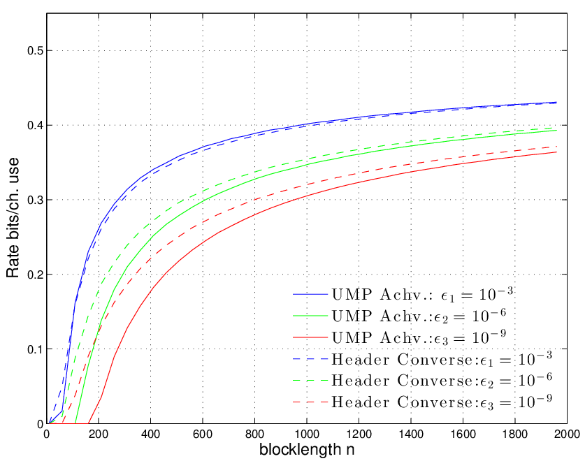
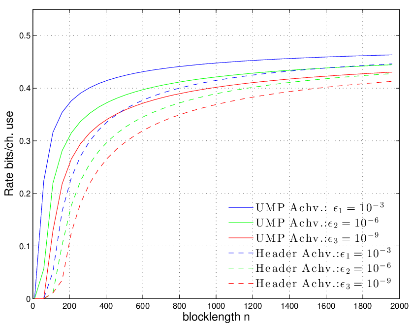
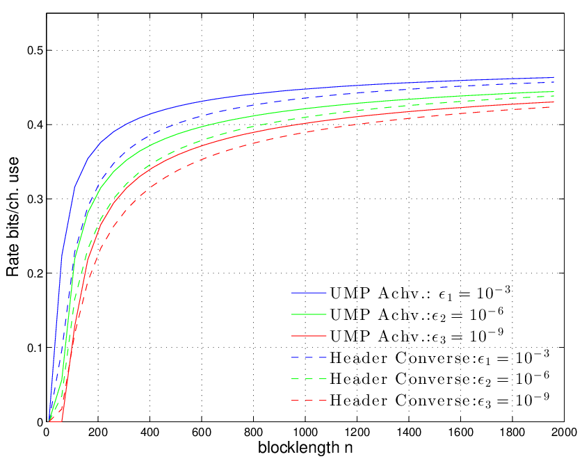
We further use this section to investigate construction of UMP codes using only existing homogeneous codes. We formally state the resulting “header bounds” based on the homogeneous DT bound in Corollaries 11 and 16 and converse “header bounds” based on the meta converse in Corollaries 13 and 17. Our plots in Figures 2 through 5 demonstrate that, in general, the header construction is suboptimal in the finite block length regime. Specifically, the plots of the BSC (resp. BEC) of UMP bounds v.s. the header achievability bound (also based on the DT bound) provided in Figure 2 (resp. Figure 4) demonstrates that the UMP codes perform much better. When we compare UMP achievability to the header converse for the BSC in Figure 3 the results are less clear. We attribute this difference to the gap between the DT bound and the converse that is presented for homogeneous codes for the BSC. Nevertheless, for the BEC for which the gap is known to be smaller, the UMP achievability bound beats the header converse bound, cf. Figure 5.

IV-A Binary Symmetric Channel

The BSC(p,np,n) is the channel from 𝖠\mathsf{A} to 𝖡\mathsf{B}, 𝖠=𝖡={0,1}n\mathsf{A}=\mathsf{B}=\{0,1\}^{n}, with stochastic kernel defined by

Wn​(yn|xn)=p|yn−xn|​(1−p)n−|yn−xn|\displaystyle W^{n}(y^{n}|x^{n})=p^{|y^{n}-x^{n}|}(1-p)^{n-|y^{n}-x^{n}|} (53)

where |yn−xn||y^{n}-x^{n}| denotes the Hamming weight of the binary vector yn−xny^{n}-x^{n}.

Corollary 10 (UMP Bound, BSC).

For any 𝛌∈ℒm\bm{\lambda}\in\mathcal{L}_{m}, there exists an ((Mi)i=1m,(ϵi)i=1m)\left((M_{i})_{i=1}^{m},(\epsilon_{i})_{i=1}^{m}\right)-UMP code (maximum probability of error) for the BSC(p,np,n) with

ϵi≤∑t=0n(nt)​pt​(1−p)n−t​min⁡[1,Miλi​2−n​p−t​(−p)t−n].\displaystyle\epsilon_{i}\!\leq\!\sum_{t=0}^{n}\!{n\choose t}p^{t}(1-p)^{n-t}\!\min\left[\!1,\!\frac{M_{i}}{\lambda_{i}}\!2^{-n}p^{-t}(\!1\!-\!p\!)^{t-n}\!\right]\!. (54)
Proof.

Following [1] we notice that with the equiprobable input distribution on XnX^{n} the information density is iXn;Yn​(xn,yn)=n​log⁡(2−2​δ)+t​log⁡δ1−δi_{X^{n};Y^{n}}(x^{n};y^{n})=n\log(2-2\delta)+t\log\frac{\delta}{1-\delta}. The result follows by computing (32). ∎

Corollary 11 (Header Achievability Bound, BSC).

For any 0≤n0≤n0\leq n_{0}\leq n, there exists an ((Mi)i=1m,(ϵi)i=1m)\left((M_{i})_{i=1}^{m},(\epsilon_{i})_{i=1}^{m}\right)-UMP code for the BSC(p,np,n) with

ϵi\displaystyle\epsilon_{i} ≤∑t=0n0(n0t)​pt​(1−p)n0−t​min⁡[1,(m−1)​2−n0−1​p−t​(1−p)t−n0]\displaystyle\!\leq\!\sum_{t=0}^{n_{0}}{n_{0}\choose t}p^{t}(1-p)^{n_{0}-t}\min\left[1,(m-1)2^{-n_{0}-1}p^{-t}(1-p)^{t-n_{0}}\right]
+∑t=0n−n0(n−n0t)pt(1−p)(n−n0)−tmin[1,(Mi−1)2−(n−n0)−1p−t(1−p)t−(n−n0)].\displaystyle\,\,+\sum_{t=0}^{n-n_{0}}{n-n_{0}\choose t}p^{t}(1-p)^{(n-n_{0})-t}\min\left[1,(M_{i}-1)2^{-(n-n_{0})-1}p^{-t}(1-p)^{t-(n-n_{0})}\right]. (55)
Proof.

The result follows by applying [1, Theorem 34] twice: once to construct a homogenous code with mm codewords over BSC(p,n0p,n_{0}) and again to construct a homogeneous code with MiM_{i} codewords over BSC(p,n−n0p,n-n_{0}). ∎

Refer to caption
Fig. 2: Comparison for BSC(0.11,n0.11,n) of UMP Code in Corollary 10 vs. header codes in Corollary 11, with m=3m=3. For UMP Code the parameter 𝝀=(13,13,13)\bm{\lambda}=(\frac{1}{3},\frac{1}{3},\frac{1}{3}) was selected. For the header code only values of n0n_{0} that can support at least one codeword in every class were considered. The best rate across all of such codes is plotted for each class.

Letting m=1m=1 and n0=0n_{0}=0 Corollary 11 reduces to

ϵ\displaystyle\epsilon ≤∑t=0n(nt)​pt​(1−p)n−t​min⁡[1,(M−1)​2−n−1​p−t​(1−p)t−n]\displaystyle\leq\sum_{t=0}^{n}{n\choose t}p^{t}(1-p)^{n-t}\min\left[1,(M-1)2^{-n-1}p^{-t}(1-p)^{t-n}\right] (56)

which is exactly [1, Theorem 34]. Comparing (56) and (54) we can attribute the M−1M-1 term being replaced by Miλi\frac{M_{i}}{\lambda_{i}} to the presence of multiple classes in the code and 2−n−12^{-n-1} being replaced by 2−n2^{-n} to the fact that we use maximum probability of error bound to obtain Corollary 10.

Corollary 12 (UMP Converse, BSC).

Any ((Mi)i=1m,(ϵi)i=1m)\left((M_{i})_{i=1}^{m},(\epsilon_{i})_{i=1}^{m}\right)-UMP code over BSC(p,np,n) must satisfy

Mi≤λiβ1−ϵin,∀i=1,…,m and some 𝝀∈ℒm\displaystyle M_{i}\leq\frac{\lambda_{i}}{\beta_{1-\epsilon_{i}}^{n}},\quad\forall i=1,\dots,m\mbox{ and some }\bm{\lambda}\in\mathcal{L}_{m} (57)

where βαn\beta_{\alpha}^{n} is defined as

βαn\displaystyle\beta_{\alpha}^{n} =(1−ρ)​βL+ρ​βL+1\displaystyle=(1-\rho)\beta_{L}+\rho\beta_{L+1} (58)
βl\displaystyle\beta_{l} =∑j=0l(nj)​2−n,\displaystyle=\sum_{j=0}^{l}{n\choose j}2^{-n}, (59)

and where 0≤ρ≤10\leq\rho\leq 1, and the integer LL are defined by

α\displaystyle\alpha =(1−ρ)​αL+ρ​αL+1\displaystyle=(1-\rho)\alpha_{L}+\rho\alpha_{L+1} (60)
αl\displaystyle\alpha_{l} =∑j=1l−1(nj)​(1−p)n−j​pj.\displaystyle=\sum_{j=1}^{l-1}{n\choose j}(1-p)^{n-j}p^{j}. (61)
Proof.

Follows by identical reasoning to [1, Theorem 35] applied to Theorem 8. ∎

Refer to caption
Fig. 3: Comparison for BSC(0.11,n0.11,n) of UMP code in Corollary 10 vs. header code converse Corollary 13), with m=3m=3. For UMP code the parameter 𝝀=(13,13,13)\bm{\lambda}=(\frac{1}{3},\frac{1}{3},\frac{1}{3}) was selected. For the header code only values of n0n_{0} which can support at least one codeword in every class were considered. The best rate across all of such codes was plotted for each class.
Corollary 13 (Header Converse Bound, BSC).

Let βαn\beta_{\alpha}^{n} be as in (58). Then, any ((Mi)i=1m,(ϵi)i=1m)\left((M_{i})_{i=1}^{m},(\epsilon_{i})_{i=1}^{m}\right)-UMP code for the BSC(p,np,n) designed via the header construction must satisfy

m≤1β1−ϵ0n0,\displaystyle m\leq\frac{1}{\beta_{1-\epsilon_{0}}^{n_{0}}}, (62)

and

Mi\displaystyle M_{i} ≤1β1−(ϵi−ϵ0)n−n0​ if ​ϵi≥ϵ0\displaystyle\leq\frac{1}{\beta_{1-(\epsilon_{i}-\epsilon_{0})}^{n-n_{0}}}\mbox{ if }\epsilon_{i}\geq\epsilon_{0} (63)
Mi\displaystyle M_{i} =0​ otherwise,\displaystyle=0\mbox{ otherwise,} (64)

for some 0≤n0≤n0\leq n_{0}\leq n and 0≤ϵ0≤10\leq\epsilon_{0}\leq 1.

Proof.

The result follows by applying [1, Theorem 35] twice: once to construct a homogenous code with mm codewords over BSC(p,n0p,n_{0}) and again to construct a homogeneous code with MiM_{i} codewords over BSC(p,n−n0p,n-n_{0}). ∎

IV-B Binary Erasure Channel

Corollary 14 (UMP Bound, BEC).

For any 𝛌∈ℒm{\bm{\lambda}}\in\mathcal{L}_{m}, there exists an ((Mi)i=1m,(ϵi)i=1m)\left((M_{i})_{i=1}^{m},(\epsilon_{i})_{i=1}^{m}\right)-UMP code (maximum probability of error) for the BEC(p,np,n) with

ϵi≤∑t=0n(nt)​pt​(1−p)n−t​min⁡[1,Miλi​2t−n].\displaystyle\epsilon_{i}\leq\sum_{t=0}^{n}{n\choose t}p^{t}(1-p)^{n-t}\min\left[1,\frac{M_{i}}{\lambda_{i}}2^{t-n}\right]. (65)
Proof.

Following [1] we notice that with the equiprobable input distribution on XnX^{n} the information density is

iXn;Yn(xn;yn)={#⁡{j:yj≠e}⋅log⁡2, if yn and xn agree on non-erased positions,−∞, otherwise.\displaystyle i_{X^{n};Y^{n}}(x^{n};y^{n})=\left\{\begin{array}[]{l}\#\{j:y_{j}\neq e\}\cdot\log 2,\\ \quad\mbox{ if $y^{n}$ and $x^{n}$ agree on non-erased}\\ \quad\mbox{ positions,}\\ -\infty,\mbox{ otherwise.}\end{array}\right.

The result follows by computing (32). ∎

Corollary 15 (UMP Converse, BEC).

Any ((Mi)i=1m,(ϵi)i=1m)\left((M_{i})_{i=1}^{m},(\epsilon_{i})_{i=1}^{m}\right)-UMP code over BEC(p,np,n) must satisfy

ϵi≥∑l=0n(nl)​pl​(1−p)n−l​(1−λi​2n−lMi)+\displaystyle\epsilon_{i}\geq\sum_{l=0}^{n}{n\choose l}p^{l}(1-p)^{n-l}\left(1-\frac{\lambda_{i}2^{n-l}}{M_{i}}\right)^{+} (70)

for some 𝛌∈ℒm\bm{\lambda}\in\mathcal{L}_{m}.

Proof.

Follows by combining Theorem 8 and [20, Theorem 23]. ∎

Corollary 16 (Header Achievability Bound, BEC).

For any 0≤n0≤n0\leq n_{0}\leq n, there exists an ((Mi)i=1m,(ϵi)i=1m)\left((M_{i})_{i=1}^{m},(\epsilon_{i})_{i=1}^{m}\right)-UMP code (maximum probability of error) for the BEC(p,np,n) with

ϵi\displaystyle\epsilon_{i} ≤∑t=0n0(nt)​pt​(1−p)n0−t​min⁡[1,(m−1)​2t−n0−1]\displaystyle\leq\sum_{t=0}^{n_{0}}{n\choose t}p^{t}(1-p)^{n_{0}-t}\min\left[1,(m-1)2^{t-n_{0}-1}\right]
+∑t=0n−n0((n−n0)t)pt(1−p)(n−n0)−tmin[1,(Mi−1)2t−(n−n0)−1].\displaystyle\qquad+\sum_{t=0}^{n-n_{0}}{(n-n_{0})\choose t}p^{t}(1-p)^{(n-n_{0})-t}\min\left[1,(M_{i}-1)2^{t-(n-n_{0})-1}\right]. (71)
Proof.

The result follows by applying [1, Theorem 37] twice: once to construct a homogenous code with mm codewords over BEC(p,n0p,n_{0}) and again to construct a homogeneous code with MiM_{i} codewords over BEC(p,n−n0p,n-n_{0}). ∎

Refer to caption
Fig. 4: Comparison for BEC(0.5,n0.5,n) of UMP code in Corollary 14 vs. header codes in Corollary 16, with m=3m=3. For the UMP code the parameter 𝝀=(13,13,13)\bm{\lambda}=(\frac{1}{3},\frac{1}{3},\frac{1}{3}) was selected. For the header code only values of n0n_{0} that can support at least one codeword in every class were considered. The best rate across all of such codes is plotted for each class.

Letting m=1m=1 and n0=0n_{0}=0 Corollary 16 reduces to

ϵ\displaystyle\epsilon ≤∑t=0n(nt)​pt​(1−p)n−t​min⁡[1,(M−1)​2t−n−1]\displaystyle\leq\sum_{t=0}^{n}{n\choose t}p^{t}(1-p)^{n-t}\min\left[1,(M-1)2^{t-n-1}\right] (72)

which is exactly [1, Theorem 37]. Comparing (72) and (65) we can again attribute the M−1M-1 term being replaced by Miλi\frac{M_{i}}{\lambda_{i}} to the presence of multiple classes in the code and 2t−n−12^{t-n-1} being replaced by 2t−n2^{t-n} to the fact that we use maximum probability of error bound to obtain Corollary 14.

Corollary 17 (Header Converse Bound, BEC).

Any ((Mi)i=1m,(ϵi)i=1m)\left((M_{i})_{i=1}^{m},(\epsilon_{i})_{i=1}^{m}\right)-UMP code over BEC(p,np,n) must satisfy

ϵi≥∑l=0n0(n0l)​pl​(1−p)n0−l​(1−2n0−lm)++∑l=0n−n0(n−n0l)​pl​(1−p)(n−n0)−l​(1−2(n−n0)−lMi)+\displaystyle\epsilon_{i}\geq\sum_{l=0}^{n_{0}}{n_{0}\choose l}p^{l}(1-p)^{n_{0}-l}\left(1-\frac{2^{n_{0}-l}}{m}\right)^{+}+\sum_{l=0}^{n-n_{0}}{n-n_{0}\choose l}p^{l}(1-p)^{(n-n_{0})-l}\left(1-\frac{2^{(n-n_{0})-l}}{M_{i}}\right)^{+} (73)

for some 0≤n0≤n0\leq n_{0}\leq n.

Proof.

The result follows by applying [1, Theorem 38] twice: once to construct a homogenous code with mm codewords over BEC(p,n0p,n_{0}) and again to construct a homogeneous code with MiM_{i} codewords over BEC(p,n−n0p,n-n_{0}). ∎

IV-C On Achievability via Coset Codes

In this section we address the use of coset codes to construct UMP codes. Motivated by the coset construction of [19] we present a construction where the UMP code is a union of coset codes. This allows efficient encoding. To decode it is, in general, necessary to decode with respect to every sub-code. Thus, decoding complexity scales with the number of message classes, mm.

Refer to caption
Fig. 5: Comparison for BEC(0.5,n0.5,n) of UMP Code in Corollary 14 vs. Header Codes converse (in Corollary 16), with m=3m=3. For UMP Code the parameter 𝝀=(13,13,13)\bm{\lambda}=(\frac{1}{3},\frac{1}{3},\frac{1}{3}) was selected. For the header code only values of n0n_{0} which can support at least one codeword in every class were considered. The best rate across all of such codes was plotted for each class.
Theorem 18 (Achievability via Coset Codes).

Let k1,…,kmk_{1},\dots,k_{m} be mm positive integers and define

Mi=2ki,i∈{1,2,…,m}.\displaystyle M_{i}=2^{k_{i}},\quad i\in\{1,2,\dots,m\}.

Then for any 𝛌∈ℒm\bm{\lambda}\in\mathcal{L}_{m} there exists an ((Mi)i=1m,(ϵi)i=1m)\left((M_{i})_{i=1}^{m},(\epsilon_{i})_{i=1}^{m}\right)-UMP code (average probability of error) where 𝒞=⋃𝒞i\mathcal{C}=\bigcup\mathcal{C}_{i} over BSC(p,np,n) (respectively, BEC(p,np,n)) satisfying (54) (respectively, (65)) such that each subcode 𝒞i\mathcal{C}_{i} is a coset of some linear code.

Proof.

We will show that under the stated conditions, we can construct 𝒞1,𝒞2,…,𝒞m\mathcal{C}_{1},\mathcal{C}_{2},\dots,\mathcal{C}_{m} such that 𝒞\mathcal{C} satisfies (30). The rest of the Theorem follows since (54) and (65) can be obtained by specializing (30) appropriately.

Code Construction: We will construct the code as follows: Let GiG_{i} be a ki×nk_{i}\times n generator matrix and viv_{i} be a 1×n1\times n coset shift. Define ℳi:={ui:ui​ is a ​1×ki​ binary vector}\mathcal{M}_{i}:=\{u_{i}:u_{i}\mbox{ is a }1\times k_{i}\mbox{ binary vector}\}. Then 𝒞i:={ui​Gi+vi:ui∈ℳi}\mathcal{C}_{i}:=\{u_{i}G_{i}+v_{i}:u_{i}\in\mathcal{M}_{i}\} where multiplications and additions are over 𝔽2\mathbb{F}_{2}.

To show such code exists we sequentially generate each (Gi,vi)(G_{i},v_{i}) independently at random starting with (G1,v1)(G_{1},v_{1}). We will show that the resulting code has good error properties and select some (Gi,vi)(G_{i},v_{i}) from the ensemble that meets the expected performance.

Decoding Rule: We use a sequential threshold decoder, as in the UMP dependence testing bound,

𝗀⁡(yn):=arg​mini,w⁡{ci,w:iXn;Yn​(ci,w,yn)>log⁡τi},\displaystyle\mathsf{g}(y^{n})\!:=\!\argmin_{i,w}\left\{c_{i,w}:i_{X^{n};Y^{n}}(c_{i,w};y^{n})\!>\!\log\tau_{i}\right\}, (74)

where i∈{1,2,…,m}i\in\{1,2,\dots,m\}, w∈{1,2,…,Mi}w\in\{1,2,\dots,M_{i}\}, τi=Miλi\tau_{i}=\frac{M_{i}}{\lambda_{i}} for all ii, PXn,Yn​(xn,yn)=PXn​(xn)​Wn​(yn|xn)P_{X^{n},Y^{n}}(x^{n},y^{n})=P_{X^{n}}(x^{n})W^{n}(y^{n}|x^{n}) and PXnP_{X^{n}} is the uniform distribution on 𝔽2n\mathbb{F}_{2}^{n}.

Error Analysis: We will prove that the error for 𝒞\mathcal{C} satisfies (30) by induction on sub-codes. Consider the base case, i=1i=1. We generate entries of G1G_{1} and v1v_{1} in an i.i.d. manner according to a Bernoulli(12\frac{1}{2}) distribution. Let c1,1=u1​G1+v1c_{1,1}=u_{1}G_{1}+v_{1} be the codeword sent and u~1​G1+v1\tilde{u}_{1}G_{1}+v_{1} be some other codeword. The two codewords are pairwise independent and so we have that for some G1G_{1} and v1v_{1},

ϵ1\displaystyle\epsilon_{1} ≤ℙ[iXn;Yn(Xn;Yn)≤logτ1]+(M1−1)ℙ[iXn;Yn(X¯n;Yn)>logτ1]\displaystyle\leq\mathbb{P}\left[i_{X^{n};Y^{n}}(X^{n};Y^{n})\leq\log\tau_{1}\right]+(M_{1}-1)\mathbb{P}\left[i_{X^{n};Y^{n}}(\bar{X}^{n};Y^{n})>\log\tau_{1}\right] (75)

where PX¯n;Yn​(xn,yn)=PXn​(xn)​PXn​Wn​(yn)P_{\bar{X}^{n};Y^{n}}(x^{n},y^{n})=P_{X^{n}}(x^{n})P_{X^{n}}W^{n}(y^{n}).

Now, suppose (G1,v1),…,(Gi−1,vi)(G_{1},v_{1}),\dots,(G_{i-1},v_{i}) are fixed. Generate entries of (Gi,vi)(G_{i},v_{i}) in an i.i.d. manner according to a Bernoulli(12\frac{1}{2}) distribution. Suppose the random vector ui​Gi+viu_{i}G_{i}+v_{i} is the true codeword sent. Then the probability that the information density of the true codeword and the output vector is lower than the decoding threshold is bounded by,

ℙ[iXn;Yn(uiGi+vi;Yn)≤logτi]=ℙ[iXn;Yn(Xn;Yn)≤logτi].\displaystyle\mathbb{P}\left[i_{X^{n};Y^{n}}(u_{i}G_{i}+v_{i};Y^{n})\leq\log\tau_{i}\right]=\mathbb{P}\left[i_{X^{n};Y^{n}}(X^{n};Y^{n})\leq\log\tau_{i}\right]. (76)

The probability of confusing ui​Gi+viu_{i}G_{i}+v_{i} with some other u~i​Gi+vi\tilde{u}_{i}G_{i}+v_{i} is, by pairwise independence and the uniform distribution induced,

ℙ[iXn;Yn(u~iGi+vi;Yn)>logτi|u~i≠ui]=ℙ[i(X¯n;Yn)>logτi].\displaystyle\mathbb{P}\left[\left.i_{X^{n};Y^{n}}(\tilde{u}_{i}G_{i}+v_{i};Y^{n})>\log\tau_{i}\right|\tilde{u}_{i}\neq u_{i}\right]=\mathbb{P}\left[i(\bar{X}^{n};Y^{n})>\log\tau_{i}\right]. (77)

Finally to bound the probability of confusion with x~n=u~j​Gj+vj\tilde{x}^{n}=\tilde{u}_{j}G_{j}+v_{j}, a codeword in another class j<ij<i, observe that ui​Gi+viu_{i}G_{i}+v_{i} induces an equiprobable distribution on YnY^{n} and

ℙ[iXn;Yn(x~n;Yn)>logτj]≤supxn∈𝖠ℙ[iXn;Yn(xn;Yn)>logτj].\displaystyle\mathbb{P}\left[i_{X^{n};Y^{n}}(\tilde{x}^{n};Y^{n})>\log\tau_{j}\right]\leq\sup_{x^{n}\in\mathsf{A}}\mathbb{P}\left[i_{X^{n};Y^{n}}(x^{n};Y^{n})>\log\tau_{j}\right]. (78)

Since, given a random (Gi,vi)(G_{i},v_{i}) pair a codeword ui​Gi+viu_{i}G_{i}+v_{i} satisfies these bounds for all ui∈ℳiu_{i}\in\mathcal{M}_{i}, the error averaged over all codewords must too. So there must exist a (Gi,vi)(G_{i},v_{i}) pair such that

ϵi\displaystyle\epsilon_{i} ≤ℙ[iXn;Yn(Xn;Yn)≤logτi]+(Mi−1)supxℙ[iXn;Yn(xn;Yn)>logτi]\displaystyle\leq\mathbb{P}\left[i_{X^{n};Y^{n}}(X^{n};Y^{n})\leq\log\tau_{i}\right]+(M_{i}-1)\sup_{x}\mathbb{P}\left[i_{X^{n};Y^{n}}(x^{n};Y^{n})>\log\tau_{i}\right]
+∑j=1i−1Mjsupxℙ[iXn;Yn(xn;Yn)>logτj]\displaystyle\quad+\sum_{j=1}^{i-1}M_{j}\sup_{x}\mathbb{P}\left[i_{X^{n};Y^{n}}(x^{n};Y^{n})>\log\tau_{j}\right] (79)

which shows (30) for equiprobable PXnP_{X^{n}} and is sufficient to show (54) for the BSC and (65) for the BEC. ∎

V Asymptotic Theorems

In this section we state two asymptotic theorems for the DMC. We analyze fixed error asymptotics and moderate deviations asymptotics for UMP codes and show that in both cases the performance loss compared to a homogeneous code with equivalent parameters is captured by some Λ∈ℒ\Lambda\in\mathcal{L} (cf. equation (24)).

In our theorem statements we allow the number of classes mnm_{n} to scale as a function of block length. One motivation for such scaling is the use of UMP codes for joint source-channel codes as in [3]. Note that in [3] the number of UMP classes needed is connected with the the number of type classes of the source. Thus, for a discrete memoryless source mnm_{n} scales as a polynomial in block length. Examples of other interesting sources include [21], where the number of type classes scales exponentially in n\sqrt{n}.

Recall that WnW^{n} is a DMC with input alphabet 𝒜\mathcal{A} and output alphabet ℬ\mathcal{B} if we can write,

Wn​(yn|xn)=∏j=1nW⁡(yj|xj).\displaystyle W^{n}(y^{n}|x^{n})=\prod_{j=1}^{n}W(y_{j}|x_{j}). (80)

We will apply single-shot bounds of Section III taking WnW^{n} as the channel. We take 𝖠=𝒜n\mathsf{A}=\mathcal{A}^{n} (respectively 𝖡=ℬn\mathsf{B}=\mathcal{B}^{n}) to be the channel input (respectively output) alphabet.

Theorem 19 (Fixed Error UMP Asymptotics).

Suppose that WW is such that V⁡(PX∗,W)>0V(P^{\ast}_{X},W)>0 for all PX∗∈ΠP^{\ast}_{X}\in\Pi. Let

  • •

    mnm_{n} be a sequence of class sizes (growing arbitrarily fast) in nn,

  • •

    ϵi\epsilon_{i} be a sequence of error probabilities such that

    infi∈ℕϵi>0​ and ​supi∈ℕϵi<1.\displaystyle\inf_{i\in\mathbb{N}}\epsilon_{i}>0\mbox{ and }\sup_{i\in\mathbb{N}}\epsilon_{i}<1.

Then, for any Λ∈ℒ\Lambda\in\mathcal{L} there is a sequence of ((Mn,i)i=1mn,(ϵi)i=1mn)\left((M_{n,i})_{i=1}^{m_{n}},(\epsilon_{i})_{i=1}^{m_{n}}\right)-UMP codes such that

log⁡Mn,i≥n​C−n​Vϵi​Q−1​(ϵi)+θi​(n)−log⁡1Λn,i.\displaystyle\log M_{n,i}\geq nC-\sqrt{nV_{\epsilon_{i}}}Q^{-1}(\epsilon_{i})+\theta_{i}(n)-\log\frac{1}{\Lambda_{n,i}}. (81)

Conversely, any sequence of ((Mn,i)i=1mn,(ϵi)i=1mn)\left((M_{n,i})_{i=1}^{m_{n}},(\epsilon_{i})_{i=1}^{m_{n}}\right)-UMP codes must satisfy

log⁡Mn,i≤n​C−n​Vϵi​Q−1​(ϵi)+θ~i​(n)−log⁡1Λn,i\displaystyle\log M_{n,i}\leq nC-\sqrt{nV_{\epsilon_{i}}}Q^{-1}(\epsilon_{i})+\tilde{\theta}_{i}(n)-\log\frac{1}{\Lambda_{n,i}} (82)

for some Λ∈ℒ\Lambda\in\mathcal{L}.

The remainder terms θi​(n)\theta_{i}(n) and θ~i\tilde{\theta}_{i} satisfy

K⁡(e¯,e¯,W)≤θi​(n)​ and ​θ~i≤12​log⁡n+K¯​(e¯,e¯,W)\displaystyle K(\underline{e},\overline{e},W)\leq\theta_{i}(n)\mbox{ and }\tilde{\theta}_{i}\leq\frac{1}{2}\log n+\bar{K}(\underline{e},\overline{e},W) (83)

where e¯=infi∈ℕϵi\underline{e}=\inf_{i\in\mathbb{N}}\epsilon_{i}, e¯=supi∈ℕϵi\overline{e}=\sup_{i\in\mathbb{N}}\epsilon_{i}, and K⁡(e¯,e¯,W),K¯​(e¯,e¯,W)K(\underline{e},\overline{e},W),\bar{K}(\underline{e},\overline{e},W) are constants which depend on e¯\underline{e}, e¯\overline{e}, and WW.

If WW is symmetric and singular in the sense of [15] the remainder terms for the achievability statement further satisfy

θi​(n)≤K¯​(e¯,e¯,W).\displaystyle\theta_{i}(n)\leq\bar{K}(\underline{e},\overline{e},W). (84)

The proof outline is as follows. We follow the approach of [1, Theorem 45]. To show achievability we use the UMP achievability bound of Theorem 2 and bound each term in (30) using the Berry-Esseen theorem. The converse follows by using Theorem 8 together with the approach of Tomamichel and Tan [14] to obtain (83) and the approach of Altuğ and Wagner [15] to obtain (84). See Appendix C for proof.

Remark 1.

For m=1m=1 Theorem 19 reduces to the best results known in literature for most DMCs. A notable exception is the achievability bound when WW is non-singular for which [2] showed using the RCU bound that

12​log⁡n+K⁡(e¯,e¯,W)≤θi​(n).\displaystyle\frac{1}{2}\log n+K(\underline{e},\overline{e},W)\leq\theta_{i}(n). (85)

This extension is not possible in our case due to the previously mentioned difficulty of extending the RCU bound to the framework of UMP codes.

For a general DMC and mm growing faster than poly⁡(n)\poly(n), there is a tradeoff in the sizes of different message classes of a UMP code. Two particularly interesting regimes are mm growing exponentially in n\sqrt{n} and mm growing exponentially in nn. In these two regimes the tradeoffs are in the dispersion and capacity terms (respectively).

For a symmetric singular DMC and mm growing as a function of nn there is a tradeoff in the sizes of different message classes of a UMP code. A particular regime of interest is mn=poly⁡(n)m_{n}=\poly(n) where the tradeoffs become apparent in the third-order O⁡(log⁡n)O(\log n) term. For mm constant no meaningful results can be proved since the current normal approximations do not quantify the constant term even for homogeneous codes.

To state our next result we define a number of regularity conditions on two positive sequences ((ρn)n=1∞,(λn)n=1∞)\left((\rho_{n})_{n=1}^{\infty},(\lambda_{n})_{n=1}^{\infty}\right).

  1. 1.

    The “homogenous” moderate deviations condition is satisfied if

    ρn→0, and ​n​ρn2→∞\displaystyle\rho_{n}\to 0,\mbox{ and }n\rho_{n}^{2}\to\infty (86)
  2. 2.

    The “positivity conditions” is satisfied if

    (ρn−λn)>0\displaystyle(\rho_{n}-\lambda_{n})>0 (87)

    for all nn sufficiently large.

  3. 3.

    The “speed of convergence” condition is satisfied if

    lim infn→∞n​(ρn−λn)2=∞.\displaystyle\liminf_{n\to\infty}n(\rho_{n}-\lambda_{n})^{2}=\infty. (88)

Note, the fact that λn>0\lambda_{n}>0 for nn sufficiently large together with homogeneous and positivity conditions imply (ρn−λn)→0(\rho_{n}-\lambda_{n})\to 0. Sequences that satisfy all three of these conditions are said to satisfy moderate deviations regularity conditions.

Theorem 20 (Moderate Deviations UMP Asymptotics).

Suppose that WW is such that V⁡(PX∗,W)>0V(P^{\ast}_{X},W)>0 for all PX∗∈ΠP^{\ast}_{X}\in\Pi. Fix Λ∈ℒ\Lambda\in\mathcal{L} and a collections of sequences ((ρn,i)n=1∞)i=1∞\left((\rho_{n,i})_{n=1}^{\infty}\right)_{i=1}^{\infty} such that for each ii the pair of sequences ((ρn,i)n=1∞,(1n​log⁡1Λn,i)n=1∞)\left((\rho_{n,i})_{n=1}^{\infty},\left(\frac{1}{n}\log\frac{1}{\Lambda_{n,i}}\right)_{n=1}^{\infty}\right) satisfy moderate deviations regularity conditions. Then, there exists a sequence of ((Mn,i)i=1mn,(ϵn,i)i=1mn)\left((M_{n,i})_{i=1}^{m_{n}},(\epsilon_{n,i})_{i=1}^{m_{n}}\right)-UMP codes satisfying

Mn,i=⌊2n​C−n​ρn,i⌋\displaystyle M_{n,i}=\lfloor 2^{nC-n\rho_{n,i}}\rfloor (89)

and

lim supn→∞1n​(ρn,i−1n​log⁡1Λn,i)2​log⁡ϵn,i≤−12​Vmin.\displaystyle\limsup_{n\to\infty}\frac{1}{n(\rho_{n,i}-\frac{1}{n}\log\frac{1}{\Lambda_{n,i}})^{2}}\log\epsilon_{n,i}\leq-\frac{1}{2V_{\min}}. (90)

Conversely, consider a sequence of ((Mn,i)i=1mn,(ϵn,i)i=1mn)\left((M_{n,i})_{i=1}^{m_{n}},(\epsilon_{n,i})_{i=1}^{m_{n}}\right)-UMP codes satisfying  (86) and (89). Then, there exists some Λ∈ℒ\Lambda\in\mathcal{L} such that for each ii the following holds:

  • •

    if ((ρn,i)n=1∞,(1n​log⁡1Λn,i)n=1∞)\left((\rho_{n,i})_{n=1}^{\infty},\left(\frac{1}{n}\log\frac{1}{\Lambda_{n,i}}\right)_{n=1}^{\infty}\right) satisfies moderate deviations regularity conditions then,

    lim infn→∞1n​(ρn,i−1n​log⁡1Λn,i)2​log⁡ϵn,i≥−12​Vmin,\displaystyle\liminf_{n\to\infty}\frac{1}{n(\rho_{n,i}-\frac{1}{n}\log\frac{1}{\Lambda_{n,i}})^{2}}\log\epsilon_{n,i}\geq-\frac{1}{2V_{\min}}, (91)
  • •

    otherwise

    lim infn→∞ϵn,i>0.\displaystyle\liminf_{n\to\infty}\epsilon_{n,i}>0. (92)

Here the tradeoffs are not apparent if mnm_{n} growing exponentially in n\sqrt{n} since then 1n​log⁡1Λn,i=o⁡(ρn,i)\frac{1}{n}\log\frac{1}{\Lambda_{n,i}}=o(\rho_{n,i}) for all valid ρn,i\rho_{n,i}. If it is growing any faster, however, we can observe degradation in the speed of convergence to the moderate deviations exponent. Thus, the moderate deviations setting interpolates the loss observed for fixed error asymptotic and error exponent regimes.

VI Concluding Remarks

Throughout this paper we have used the set ℒm\mathcal{L}_{m} and its asymptotic counterpart ℒ\mathcal{L} to capture the tradeoffs between different message classes in a UMP code. It may be useful to give an intuitive interpretation of the ℒm\mathcal{L}_{m} set. We interpret each element of ℒm\mathcal{L}_{m} as capturing a partitioning of ‘resources’ (e.g., decoding space) between different classes. This is the main idea behind our converse bound of Theorem 8; there the common output distribution QYQ_{Y} is used to tie the mm sub-codes together. The same parameterization appears in our achievability bounds of Corollary 3 and Theorem 4. This suggests that such resource ‘sharing’ can be accomplished in a rather efficient way. Next, we may wonder if UMP codes parameterized by one element of ℒm\mathcal{L}_{m} are better or worse than codes parameterized by another element of ℒm\mathcal{L}_{m}. To answer this question it is helpful to relate them to some operational quantity. This is discussed next.

VI-A Operational Meaning of ℒm\mathcal{L}_{m}

Recall from Section II that one measure of “goodness” proposed for UMP codes is the expected rate (see Definition 3). Suppose we fix mm error probability constraints (ϵi)i=1m(\epsilon_{i})_{i=1}^{m} and study the corresponding possible sizes of mm message classes. The finite block length bounds tell us that given the (ϵi)i=1m(\epsilon_{i})_{i=1}^{m} constraints there is a family of UMP codes parametrized by ℒm\mathcal{L}_{m}. W nat wish to maximize the expected rate over this family of codes. Ignoring the third order terms in Theorem 19 we obtain the following normal approximation for the size of each code at finite nn for a given 𝝀∈ℒm\bm{\lambda}\in\mathcal{L}_{m},

log⁡Mi≈n​C−n​V​Q−1​(ϵi)−log⁡1λi,1≤i≤m.\displaystyle\log M_{i}\approx nC-\sqrt{nV}Q^{-1}(\epsilon_{i})-\log\frac{1}{\lambda_{i}},\quad 1\leq i\leq m. (93)

Let us fix some prior probabilities (μ1,…,μm)(\mu_{1},\dots,\mu_{m}) on the mm message classes and consider maximizing the expected rate given (ϵi)i=1m(\epsilon_{i})_{i=1}^{m},

max𝝀∈ℒm⁡R⁡(𝝁)=max𝝀∈ℒm⁡1n​∑i=1mμi​(log⁡Mi−log⁡μi)\displaystyle\max_{\bm{\lambda}\in\mathcal{L}_{m}}R({\bm{\mu}})=\max_{\bm{\lambda}\in\mathcal{L}_{m}}\frac{1}{n}\sum_{i=1}^{m}\mu_{i}(\log M_{i}-\log\mu_{i}) (94)
≈max𝝀∈ℒm⁡1n​∑i=1mμi​(n​C−n​V​Q−1​(ϵi)−log⁡1λn,i−log⁡μi)\displaystyle\approx\max_{\bm{\lambda}\in\mathcal{L}_{m}}\frac{1}{n}\sum_{i=1}^{m}\mu_{i}(nC-\sqrt{nV}Q^{-1}(\epsilon_{i})-\log\frac{1}{\lambda_{n,i}}-\log\mu_{i}) (95)

The first two terms in (95) are constant since they do not involve 𝝀\bm{\lambda}. Let A=1n​∑i=1mμi​(n​C−n​Q−1​(ϵi))A=\frac{1}{n}\sum_{i=1}^{m}\mu_{i}(nC-\sqrt{n}Q^{-1}(\epsilon_{i})). Then, we have

max𝝀∈ℒm⁡R⁡(𝝁)\displaystyle\max_{\bm{\lambda}\in\mathcal{L}_{m}}R({\bm{\mu}}) =A+max𝝀∈ℒ⁡1n​∑i=1mμi​log⁡λi−1n​∑i=1mμi​log⁡μi\displaystyle=A+\max_{\bm{\lambda}\in\mathcal{L}}\frac{1}{n}\sum_{i=1}^{m}\mu_{i}\log\lambda_{i}-\frac{1}{n}\sum_{i=1}^{m}\mu_{i}\log\mu_{i} (96)
=A+1n​∑i=1mμi​log⁡μi−1n​∑i=1mμi​log⁡μi=A.\displaystyle=A+\frac{1}{n}\sum_{i=1}^{m}\mu_{i}\log\mu_{i}-\frac{1}{n}\sum_{i=1}^{m}\mu_{i}\log\mu_{i}=A. (97)

Equation (97) follows from the fact that the 𝝀\bm{\lambda} that maximizes the expected rate over ℒm\mathcal{L}_{m} is given by proportional betting with λi=μi\lambda_{i}=\mu_{i} for all 1≤i≤m1\leq i\leq m [22, Theorem 6.1.2]. In other words, the UMP code that maximizes the expected rate given a prior message class distribution is one with λi=μi\lambda_{i}=\mu_{i}. Of course, if we pick any other code we would suffer a loss of D(𝝁||𝝀)D(\bm{\mu}||\bm{\lambda}) in terms of expected rate. A more formal study of this connection is left to future work.

VI-B Major Contributions and Future Work

The main contribution of this paper is a collection of theorems which quantify tradeoffs involved in unequal message protection in asymptotic and non-asymptotic settings. We present extensions of well known finite block length bounds to UMP codes and demonstrate that both converse and achievability bounds admit similar tradeoffs which are captured by the probability simplex ℒm\mathcal{L}_{m}. Although there is a gap between these bounds at finite block lengths (just as in the original bounds), they are shown to be tight in fixed error and moderate deviations asymptotic regimes. Our results also elucidate why tradeoffs inherent to unequal message protection were not observed in previous works on the subject. In each case this was due either to the asymptotic regime studied, the scaling of the number of classes with nn, or both. In addition to exposing some fundamental tradeoffs of channel coding with unequal message protection this paper raises a number of follow up questions.

Channels with cost: One interesting question not addressed in this paper is unequal message protection for channels with cost. Our κ​β\kappa\beta-bound extension in Theorem 4 and converse bound in Corollary 9 could be applied to this problem when the cost constraint is the same for all mm classes. However, the most general formulation of channels with cost should involve different constraints for each class. Although the extension of the κ​β\kappa\beta-bound to such a setting would be quite interesting, one would likely get more utility out of extending the DT bound with cost constraints [2, Theorem 24] using similar approach to one used in Theorem 2. Likewise, a question arises as to how evaluate a meta-converse type bound since different cost constraints would have different ‘good’ output distributions QYQ_{Y}. One possible approach is to evaluate the UMP meta-converse mm times, using the ‘best’ QYQ_{Y} for each class, and take the intersection over the regions obtained.

In general, we can expect for UMP codes with cost constraints to behave in the following way. When the cost constraints are similar we will approach results derived in this paper where the loss is captured by the set ℒm\mathcal{L}_{m}. In a case when the cost constraints are drastically different the codes will approach the no-loss setting. Consider, for example, a two-class UMP code for an AWGN channel with power constraints P1P_{1} and P2P_{2}. If P1≈P2P_{1}\approx P_{2} both sub-codes will reside on approximately the same sphere determined by the power constraint. The channel noise will thus push codewords from both sub-codes into the same decoding space. If P1<<P2P_{1}<<P_{2} they will reside on power spheres that are very far apart making it so that the two sub-codes are very easy to distinguish at the channel output.

Asymptotic theorems for mixed regimes: To motivate this asymptotic setting let us consider red alert codes studied in [12, 9]. A red alert code is a type of UMP code that has two classes. One class has a single extremely well protected “red alert” codeword. The other class has exponentially many normal codewords that have some reasonable amount of error protection. In the context of streaming communication with feedback the red alert codeword can be used to signal the decoder a potentially erroneous decision, while normal codewords are used to achieve high communication rate [8, 10, 11]. Guided by this motivation we would like the asymptotics of such a code to behave in the following way. For the red alert codeword we want the rate to be fixed (in this case at zero), and the probability of error to drop as fast as possible; this is reminiscent of the error exponent regime. For the normal codewords we can tolerate a small but non-zero error probability while we want the rate to approach capacity as fast as possible: this is exactly the setting for fixed-error asymptotics.

In this work we follow the philosophy of previous asymptotic works in[3, 12, 4] and focus our attention on sequences of codes within one regime only. For example, Theorem 19 assumes that all classes in a sequence of UMP codes have constant error probability. Likewise, in Theorem 20 we assume that the rates of all the classes approach capacity at a rate consistent with the moderate deviations setting studied in [16, 17, 18]. As the first study of tradeoffs for UMP codes this has the advantage of letting us compare our bounds to the homogeneous setting. The red alert example, however, brings up a rather subtle issue that is not present in the classical channel coding. It is entirely possible to have a sequence of UMP codes in which rates (resp. errors) of different classes approach capacity (resp. zero) at different speeds, or not at all. Moreover, in light of this example, these sequences of codes may have very interesting applications. Studying the mixed setting is, thus, a natural next step.

Construction of practical UMP codes: Due to their connection to problems like streaming communication and joint source-channel coding, UMP codes may prove to be useful communication tools. Practical design of UMP codes poses a compelling question. As we have shown in Section IV in our discussion of the header construction simply taking existing codes and combining them first to encode the message class, and then encode the message, may not yield a good enough solution. Instead, a more intricate “mixing” of codewords is desired. Understanding how to construct such codes with practical construction schemes such as LDPC, Turbo, or Polar codes poses an interesting coding problem. Likewise, constructing decoding algorithms for such codes could prove to be a separate challenge. For example, the decoding complexity for UMP codes may scale with the number of classes, as in Theorem 18. On the other hand, it may be possible to avoid such scaling through smart algebraic design.

Finally, other extensions of this problem may be of interest. A natural dual question to UMP codes would be source coding with unequal distortion criterion where some sources receive better distortion guarantees than other, an idea also proposed in [12]. The connection between UMP codes and joint source-channel coding is the most natural direction of study. The idea of using UMP codes for joint source-channel coding will be explored in further detail in subsequent work.

Appendix A Proofs for Finite Block Length Bounds

Proof of Theorem 2.

We first describe the operation of the decoder for a given UMP codebook 𝒞\mathcal{C}. Then, we outline a codebook construction based on a sequential random coding technique. The error analysis will be done simultaneously with the codebook construction.

Decoding: We will use a sequential threshold decoder. Specifically, the decoder computes ıXi;Yi​(ci,w,y)\imath_{X_{i};Y_{i}}(c_{i,w},y) for received channel output yy where ii varies from 11 to mm, and ww varies from 11 to MiM_{i}. The decoder outputs the first codeword for which ıXi;Yi​(ci,w,y)>log⁡τi​(x)\imath_{X_{i};Y_{i}}(c_{i,w},y)>\log\tau_{i}(x). Formally, the decoder is defined as

g⁡(y)=arg​mini,w⁡{ci,w:ıXi;Yi​(ci,w,y)>log⁡τi​(x)},\displaystyle g(y)=\argmin_{i,w}\left\{c_{i,w}:\imath_{X_{i};Y_{i}}(c_{i,w},y)>\log\tau_{i}(x)\right\}, (98)

where i∈{1,…,m}i\in\{1,\dots,m\} and w∈{1,…,Mi}w\in\{1,\dots,M_{i}\}.

Codebook Construction: We construct a codebook sequentially starting with codewords in class 11, then class 22, all the way to class mm. To select c1,1c_{1,1} choose xx at random with distribution PX1P_{X_{1}}. Then

𝔼[ϵ1,1(x)]=ℙ[ıX1;Y1(X1,Y1)≤logτ1(X1)].\displaystyle\mathbb{E}\left[\epsilon_{1,1}(x)\right]=\mathbb{P}\left[\imath_{X_{1};Y_{1}}(X_{1},Y_{1})\leq\log\tau_{1}(X_{1})\right]. (99)

There must exist at least one xx such that ϵ1,1(x)≤ℙ[ıX1;Y1(X1,Y1)≤logτ1(X1)]\epsilon_{1,1}(x)\leq\mathbb{P}\left[\imath_{X_{1};Y_{1}}(X_{1},Y_{1})\leq\log\tau_{1}(X_{1})\right]. Call this c1,1c_{1,1} and go on to select c1,2c_{1,2} all the way to c1,M1c_{1,M_{1}}.

Suppose the sub-codebooks for the first i−1i-1 classes, 𝒞1,…,𝒞i−1\mathcal{C}_{1},\dots,\mathcal{C}_{i-1}, have been selected, as well as ll codewords in 𝒞i\mathcal{C}_{i} for some 1≤i≤m1\leq i\leq m and 0≤l≤Mi−10\leq l\leq M_{i}-1. We show that we can add a codeword to 𝒞i\mathcal{C}_{i} without violating (30). Denote

Dj\displaystyle D_{j} =⋃w=1Mj{y:ıXi;Yi​(cj,w,y)>log⁡τj​(cj,w)},\displaystyle=\bigcup_{w=1}^{M_{j}}\left\{y:\imath_{X_{i};Y_{i}}(c_{j,w},y)>\log\tau_{j}(c_{j,w})\right\}, (100)

for 1≤j≤i−11\leq j\leq i-1 and

Di\displaystyle D_{i} =⋃w=1l{y:ıXi;Yi​(ci,w,y)>log⁡τi​(ci,w)}.\displaystyle=\bigcup_{w=1}^{l}\left\{y:\imath_{X_{i};Y_{i}}(c_{i,w},y)>\log\tau_{i}(c_{i,w})\right\}. (101)

Select ci,l+1c_{i,l+1} by choosing xx at random with distribution PXiP_{X_{i}}. Then

𝔼⁡[ϵi,l+1​(c1,1,…,ci,l,x)]\displaystyle\mathbb{E}\left[\epsilon_{i,l+1}(c_{1,1},\dots,c_{i,l},x)\right]
=ℙ[⋃j=1iDj∪{ıXi;Yi(Xi,Yi)≤logτi(Xi)}]\displaystyle=\mathbb{P}\left[\bigcup_{j=1}^{i}D_{j}\cup\left\{\imath_{X_{i};Y_{i}}(X_{i},Y_{i})\leq\log\tau_{i}(X_{i})\right\}\right] (102)
≤ℙ[ıXi;Yi(Xi,Yi)≤logτi(Xi)]+∑j=1iℙ[Dj]\displaystyle\leq\mathbb{P}\left[\imath_{X_{i};Y_{i}}(X_{i},Y_{i})\leq\log\tau_{i}(X_{i})\right]+\sum_{j=1}^{i}\mathbb{P}\left[D_{j}\right] (103)
≤ℙ[ıXi;Yi(Xi,Yi)≤logτi(Xi)]+(Mi−1)supxℙ[ıXi;Yi(x;Yj)>logτj(x)]\displaystyle\leq\mathbb{P}\left[\imath_{X_{i};Y_{i}}(X_{i},Y_{i})\leq\log\tau_{i}(X_{i})\right]+(M_{i}-1)\sup_{x}\mathbb{P}\left[\imath_{X_{i};Y_{i}}(x;Y_{j})>\log\tau_{j}(x)\right]
+∑j=1i−1Mjsupxℙ[ıXi;Yi(x,Yj)≥logτj(x)]\displaystyle\quad+\sum_{j=1}^{i-1}M_{j}\sup_{x}\mathbb{P}\left[\imath_{X_{i};Y_{i}}(x,Y_{j})\geq\log\tau_{j}(x)\right] (104)

where (103) and (104) both follow by union bound. There must be at least one xx such that ϵi,l+1​(c1,1,…,ci,l,x)\epsilon_{i,l+1}(c_{1,1},\dots,c_{i,l},x) is less than (104): call this ci,l+1c_{i,l+1}. Finally, the encoder maps wwth message in ℳi\mathcal{M}_{i} to ci,wc_{i,w}, and the decoder maps ci,wc_{i,w} to wwth message in ℳi\mathcal{M}_{i} which gives the result. ∎

Proof of Theorem 4.

We first describe the decoder for a given UMP codebook 𝒞\mathcal{C}. We then use induction on the number of message classes to show that a codebook satisfying (40) and (41) can be constructed.

Decoding: Given an output y∈𝖡y\in\mathsf{B} the decoder sequentially tests whether ci,wc_{i,w} was sent with ii running from 11 to mm, and ww running from 11 to MiM_{i}. The test for ci,wc_{i,w} is performed as a binary hypothesis test discriminating Wci,wW_{c_{i,w}} (hypothesis ℋ1\mathcal{H}_{1}) against “average noise” QYQ_{Y} (hypothesis ℋ0\mathcal{H}_{0}). Given class ii we would like to select each such test as an optimal one with the constraint P⁡(decide ​ℋ1|ℋ1)≥1−ϵi+τP(\mbox{decide }\mathcal{H}_{1}|\mathcal{H}_{1})\geq 1-\epsilon_{i}+\tau. To do this we define mm collections of random variables Zi​(x)Z_{i}(x), x∈𝖥x\in\mathsf{F} all conditionally independent given YY and with PZi​(x)|YP_{Z_{i}(x)|Y} chosen so that it achieves β1−ϵi+τ​(Wx,QY)\beta_{1-\epsilon_{i}+\tau}(W_{x},Q_{Y}). In other words,

P⁡[Zi​(x)=1|X=x]≥1−ϵi+τ,\displaystyle P\left[Z_{i}(x)=1|X=x\right]\geq 1-\epsilon_{i}+\tau, (105)
Q[Zi(x)=1]=β1−ϵi+τ(Wx,QY),\displaystyle Q\left[Z_{i}(x)=1\right]=\beta_{1-\epsilon_{i}+\tau}(W_{x},Q_{Y}), (106)

which we can do by the Newman-Pearson Lemma.

The decoder applies independent random transformations PZ1​(c1,1),…,PZ1​(c1,M1)P_{Z_{1}}(c_{1,1}),\dots,P_{Z_{1}}(c_{1,M_{1}}) to output YY, then

PZ2​(c2,1),…,PZ2​(c2,M2)P_{Z_{2}}(c_{2,1}),\dots,P_{Z_{2}}(c_{2,M_{2}}), and so on for all mm classes. It outputs the fist index (i,w)(i,w) for which Zi​(ci,w)=1Z_{i}(c_{i,w})=1.

We proceed to prove the rest of the theorem via induction.

Codebook Construction: To show the claim for m=1m=1 we have that for an UMP code with one message class

M1≥κτ​(𝖥,QY)supx∈𝖥β1−ϵ1+τ​(Wx,QY)\displaystyle M_{1}\geq\frac{\kappa_{\tau}(\mathsf{F},Q_{Y})}{\sup_{x\in\mathsf{F}}\beta_{1-\epsilon_{1}+\tau}(W_{x},Q_{Y})} (107)

by appealing to [2, Theorem 27]. It follows that there must exist and (M1,ϵ1)\left(M_{1},\epsilon_{1}\right)-UMP code satisfying (41) with 0≤λ1≤10\leq\lambda_{1}\leq 1.

Let us assume the theorem statement is true for m−1m-1 and fix arbitrary 𝝀∈ℒm\bm{\lambda}\in\mathcal{L}_{m}. By inductive hypothesis we can construct ((Mi)i=1m−1,(ϵi)i=1m−1)\left((M_{i})_{i=1}^{m-1},(\epsilon_{i})_{i=1}^{m-1}\right)-UMP code such that

Mi=⌊λi​κτ​(𝖥,QY)supx∈𝖥β1−ϵi+τ​(x,QY)⌋.\displaystyle M_{i}=\left\lfloor\frac{\lambda_{i}\kappa_{\tau}(\mathsf{F},Q_{Y})}{\sup_{x\in\mathsf{F}}\beta_{1-\epsilon_{i}+\tau}(x,Q_{Y})}\right\rfloor. (108)

If 𝒞1,…,𝒞m−1\mathcal{C}_{1},\ldots,\mathcal{C}_{m-1} are the sub-codebooks associated with this code, we can construct 𝒞m\mathcal{C}_{m} by rehashing the greedy approach of [2, Theorem 27]. Suppose jj codewords have already been selected for 𝒞m\mathcal{C}_{m} (where jj could be zero). Define

Ui\displaystyle U_{i} =max⁡{Zi​(ci,1),…,Zi​(ci,Mi)}for ​1≤i≤m−1,\displaystyle=\max\{Z_{i}(c_{i,1}),\dots,Z_{i}(c_{i,M_{i}})\}\quad\mbox{for }1\leq i\leq m-1, (109)
Vj\displaystyle V_{j} =max⁡{0,Zm​(cm,1),…,Zk​(cm,j)}.\displaystyle=\max\{0,Z_{m}(c_{m,1}),\dots,Z_{k}(c_{m,j})\}. (110)

We choose the j+1j+1-st codeword by selecting an arbitrary x∈𝖥x\in\mathsf{F} which satisfies

ℙ[Zm(x)=1,U1=⋯=Um−1=Vj=0|X=x]≥1−ϵm.\displaystyle\mathbb{P}\left[Z_{m}(x)=1,U_{1}=\dots=U_{m-1}=V_{j}=0|X=x\right]\geq 1-\epsilon_{m}. (111)

Once no such x∈𝖥x\in\mathsf{F} can be found, we stop.

Relating Error to Codebook Size: Suppose the process stops after MmM_{m} steps and let

Z=max⁡(U1,…,Um)\displaystyle Z=\max(U_{1},\dots,U_{m}) (112)

where Um=VMmU_{m}=V_{M_{m}}. This implies that for every x∈𝖥x\in\mathsf{F} we have

ℙ[Zm(x)=1,Z=0|X=x]<1−ϵm\displaystyle\mathbb{P}\left[Z_{m}(x)=1,Z=0|X=x\right]<1-\epsilon_{m} (113)

Then by definition of Zm​(x)Z_{m}(x) it follows

1−ϵm+τ≤ℙ⁡[Zm​(x)=1|X=x]\displaystyle 1-\epsilon_{m}+\tau\leq\mathbb{P}[Z_{m}(x)=1|X=x] (114)
=ℙ[Zm(x)=1,Z=0|X=x]+ℙ[Zm(x)=1,Z=1|X=x]\displaystyle=\mathbb{P}[Z_{m}(x)=1,Z=0|X=x]+\mathbb{P}[Z_{m}(x)=1,Z=1|X=x] (115)
≤ℙ[Zm(x)=1,Z=0|X=x]+ℙ[Z=1|X=x]\displaystyle\leq\mathbb{P}[Z_{m}(x)=1,Z=0|X=x]+\mathbb{P}[Z=1|X=x] (116)
<1−ϵm+ℙ⁡[Z=1|X=x].\displaystyle<1-\epsilon_{m}+\mathbb{P}[Z=1|X=x]. (117)

So, for every x∈𝖥x\in\mathsf{F}

ℙ⁡[Z=1|X=x]≥τ.\displaystyle\mathbb{P}[Z=1|X=x]\geq\tau. (118)

This is exactly the composite hypothesis test defined in (7) and

Q[Z=1]≥κτ(𝖥,QY).\displaystyle Q[Z=1]\geq\kappa_{\tau}(\mathsf{F},Q_{Y}). (119)

Finally, we can bound

Q[Z=1]=Q[⋃i=1m{Ui=1}]\displaystyle Q[Z=1]=Q\left[\bigcup_{i=1}^{m}\{U_{i}=1\}\right] (120)
≤∑i=1mQ[Ui=1]\displaystyle\leq\sum_{i=1}^{m}Q\left[U_{i}=1\right] (121)
≤∑i=1mQ[⋃w=1Mi{Zi(ci,w)=1}]\displaystyle\leq\sum_{i=1}^{m}Q\left[\bigcup_{w=1}^{M_{i}}\{Z_{i}(c_{i,w})=1\}\right] (122)
≤∑i=1m∑w=1MiQ[{Zi(ci,w)=1}]\displaystyle\leq\sum_{i=1}^{m}\sum_{w=1}^{M_{i}}Q\left[\{Z_{i}(c_{i,w})=1\}\right] (123)
=∑i=1m∑w=1Miβ1−ϵi+τ​(Wci,w,QY)\displaystyle=\sum_{i=1}^{m}\sum_{w=1}^{M_{i}}\beta_{1-\epsilon_{i}+\tau}(W_{c_{i,w}},Q_{Y}) (124)
≤∑i=1m−1Mi​supx∈𝖥β1−ϵi+τ​(Wx,QY)+Mm​supx∈𝖥β1−ϵm+τ​(Wx,QY)\displaystyle\leq\sum_{i=1}^{m-1}M_{i}\sup_{x\in\mathsf{F}}\beta_{1-\epsilon_{i}+\tau}(W_{x},Q_{Y})+M_{m}\sup_{x\in\mathsf{F}}\beta_{1-\epsilon_{m}+\tau}(W_{x},Q_{Y}) (125)
≤∑i=1m−1λi​κτ​(𝖥,QY)+Mm​supx∈𝖥β1−ϵm+τ​(Wx,QY).\displaystyle\leq\sum_{i=1}^{m-1}\lambda_{i}\kappa_{\tau}(\mathsf{F},Q_{Y})+M_{m}\sup_{x\in\mathsf{F}}\beta_{1-\epsilon_{m}+\tau}(W_{x},Q_{Y}). (126)

Thus, we conclude that

Mm​supx∈𝖥β1−ϵm+τ​(Wx,QY)≥λm​κτ​(𝖥,QY)\displaystyle M_{m}\sup_{x\in\mathsf{F}}\beta_{1-\epsilon_{m}+\tau}(W_{x},Q_{Y})\geq\lambda_{m}\kappa_{\tau}(\mathsf{F},Q_{Y}) (127)

and that there exists an UMP code with mm classes of codewords satisfying (40) and (41). ∎

Proof of Theorem 5.

To show (42) we generate the codewords in each sub-code 𝒞i\mathcal{C}_{i} as independent random variables with common distribution PXiP_{X_{i}} and use the decoding rule defined in (98). Let E⁡(𝝁)E(\bm{\mu}) be the random variable denoting the expected error and EiE_{i} the random variable denoting the average error for class ii across the ensemble of all codebooks. Then

𝔼⁡[E⁡(𝝁)]=𝔼⁡[∑i=1mμi​Ei]=∑i=1mμi​𝔼​[Ei].\displaystyle\mathbb{E}[E(\bm{\mu})]=\mathbb{E}\left[\sum_{i=1}^{m}\mu_{i}E_{i}\right]=\sum_{i=1}^{m}\mu_{i}\mathbb{E}\left[E_{i}\right]. (128)

The average error for each class can be bound as

𝔼⁡[Ei]\displaystyle\mathbb{E}[E_{i}] ≤ℙ[ıXi;Yi(Xi;Yi)≤logτi(Xi)]+(Mi−1)ℙ[ıXi;Yi(X¯i;Yi)>logτi(x)]\displaystyle\leq\mathbb{P}\left[\imath_{X_{i};Y_{i}}(X_{i};Y_{i})\leq\log\tau_{i}(X_{i})\right]+(M_{i}-1)\mathbb{P}\left[\imath_{X_{i};Y_{i}}(\bar{X}_{i};Y_{i})>\log\tau_{i}(x)\right]
+∑j=1i−1Mjℙ[ıXj;Yj(Xj;Yi)>logτj(x)]\displaystyle\quad+\sum_{j=1}^{i-1}M_{j}\mathbb{P}\left[\imath_{X_{j};Y_{j}}(X_{j};Y_{i})>\log\tau_{j}(x)\right] (129)

where PX¯i,Yi​(x,y)=PXi​(x)​PXi​W​(y)P_{\bar{X}_{i},Y_{i}}(x,y)=P_{X_{i}}(x)P_{X_{i}}W(y) and PXj,Yi​(x,y)=PXj​(x)​PXi​W​(y)P_{X_{j},Y_{i}}(x,y)=P_{X_{j}}(x)P_{X_{i}}W(y) as in [1, Theorem 18]. Following reasoning similar to Corollary 3 we obtain

𝔼⁡[Ei]≤𝔼⁡[exp⁡{−[ıXi;Yi​(Xi,Yi)−log⁡Miλi]+}].\displaystyle\mathbb{E}[E_{i}]\leq\mathbb{E}\left[\exp\left\{-\left[\imath_{X_{i};Y_{i}}(X_{i};Y_{i})-\log\frac{M_{i}}{\lambda_{i}}\right]^{+}\right\}\right]. (130)

Combining (128) with (130) gives the result and applying Shannon’s argument we conclude that there exists a code satisfying (42). ∎

Proof of Theorem 6.

To show (43) we generate the codewords in each subcode 𝒞i\mathcal{C}_{i} as independent random variables with common distribution PXiP_{X_{i}}. Denote the codewords in class ii by Xi,1,…,Xi,MiX_{i,1},\dots,X_{i,M_{i}}. Our decoding rule is to pick the codeword with largest biased information density,

arg​maxi,w⁡{log⁡τi+ıXi;Yi​(Xi,w,Yi)}\displaystyle\argmax_{i,w}\left\{\log\tau_{i}+\imath_{X_{i};Y_{i}}(X_{i,w};Y_{i})\right\} (131)

where i∈{1,2,…,m}i\in\{1,2,\dots,m\} and w∈{1,2,…,Mi}w\in\{1,2,\dots,M_{i}\}. Let E⁡(𝝁)E(\bm{\mu}) be the random variable denoting the expected error and EiE_{i} the random variable denoting the average error for class ii across the ensamble of all codebooks. Then

𝔼⁡[E⁡(𝝁)]=𝔼⁡[∑i=1mμi​Ei]=∑i=1mμi​𝔼​[Ei].\displaystyle\mathbb{E}[E(\bm{\mu})]=\mathbb{E}\left[\sum_{i=1}^{m}\mu_{i}E_{i}\right]=\sum_{i=1}^{m}\mu_{i}\mathbb{E}\left[E_{i}\right]. (132)

To bound the average error for each class suppose the first codeword from class ii was sent. An error occurs only if the biased information density for some other codeword. By symmetry we obtain

𝔼⁡[Ei]\displaystyle\mathbb{E}[E_{i}] ≤ℙ[⋃j=1m⋃w=1,(j,w)≠(i,1)Mj{logτj+ıXj;Yj(X¯j,w,Yi)≥logτi+ıXi;Yi(Xi,1,Yi,1)}]\displaystyle\leq\mathbb{P}\left[\bigcup_{j=1}^{m}\bigcup_{\begin{array}[]{c}w=1,\\ (j,w)\neq(i,1)\end{array}}^{M_{j}}\big\{\log\tau_{j}+\imath_{X_{j};Y_{j}}(\bar{X}_{j,w},Y_{i})\geq\log\tau_{i}+\imath_{X_{i};Y_{i}}(X_{i,1},Y_{i,1})\big\}\right]
=𝔼[ℙ[⋃j=1m⋃w=1,(j,w)≠(i,1)Mj{ıXj;Yj(X¯j,m;Yi)≥(logτi−logτj)+ıXi;Yi(Xi,1;Yi)}|Xi,1,Yi,1]]\displaystyle=\mathbb{E}\left[\mathbb{P}\left[\left.\bigcup_{j=1}^{m}\bigcup_{\begin{array}[]{c}w=1,\\ (j,w)\neq(i,1)\end{array}}^{M_{j}}\left\{\imath_{X_{j};Y_{j}}(\bar{X}_{j,m};Y_{i})\geq(\log\tau_{i}-\log\tau_{j})+\imath_{X_{i};Y_{i}}(X_{i,1};Y_{i})\right\}\right|X_{i,1},Y_{i,1}\right]\right]
≤𝔼[min{1,∑j=1m(Mj−𝟙{1≠j})ℙ[{ıXj;Yj(X¯j,Yi)≥(logτi−logτj)+ıXi;Yi(Xi,Yi)}|Xi,Yi]}].\displaystyle\leq\mathbb{E}\left[\min\left\{1,\sum_{j=1}^{m}\left(M_{j}-\mathds{1}\left\{1\neq j\right\}\right)\mathbb{P}\left[\left.\left\{\imath_{X_{j};Y_{j}}(\bar{X}_{j},Y_{i})\geq(\log\tau_{i}-\log\tau_{j})+\imath_{X_{i};Y_{i}}(X_{i},Y_{i})\right\}\right|X_{i},Y_{i}\right]\right\}\right]. (137)

Combining (132) with (137) we get

𝔼[ϵ(𝝁)]≤∑i=1mμi𝔼[min{1,∑j=1m(Mj−1i≠j)ℙ[{ıXj;Yj(X¯j,Yi)≥(logτi−logτj)+ıXi;Yi(Xi,Yi)}|Xi,Yi]}]\displaystyle\mathbb{E}[\epsilon(\bm{\mu})]\leq\sum_{i=1}^{m}\mu_{i}\mathbb{E}\left[\min\left\{1,\sum_{j=1}^{m}\left(M_{j}-1_{i\neq j}\right)\mathbb{P}\left[\left.\left\{\imath_{X_{j};Y_{j}}(\bar{X}_{j},Y_{i})\geq(\log\tau_{i}-\log\tau_{j})+\imath_{X_{i};Y_{i}}(X_{i},Y_{i})\right\}\right|X_{i},Y_{i}\right]\right\}\right] (138)

and conclude that there exists at least one codebook with ϵ⁡(𝝁)\epsilon(\bm{\mu}) satisfying (43). ∎

Appendix B Utility Theorems

We use the theorems in this section to prove our asymptotic results. All theorems have the following common set up.

Let ZjZ_{j}, j=1,…,nj=1,\dots,n be independent random variables with

μj=𝔼⁡[Zj],σj2=V​a​r​[Zj],and ​tj=𝔼⁡[|Zj−μj|3].\displaystyle\mu_{j}=\mathbb{E}[Z_{j}],\quad\sigma_{j}^{2}=Var[Z_{j}],\quad\mbox{and }t_{j}=\mathbb{E}[|Z_{j}-\mu_{j}|^{3}]. (139)

Denote V=∑1nσj2V=\sum_{1}^{n}\sigma_{j}^{2} and T=∑1ntjT=\sum_{1}^{n}t_{j}.

Theorem 21 (Berry-Esseen).
|ℙ[∑j=1n(Zj−μj)V≤λ]−Q(−λ)|≤TV3/2\displaystyle\left|\mathbb{P}\left[\frac{\sum_{j=1}^{n}(Z_{j}-\mu_{j})}{\sqrt{V}}\leq\lambda\right]-Q(-\lambda)\right|\leq\frac{T}{V^{3/2}} (140)

The following theorem is a refined version of the Berry-Esseen theorem.

Theorem 22 (Rozovsky).

Assume ZjZ_{j} have finite third moments, that is tj<∞t_{j}<\infty. Then there exist universal constants A1>0A_{1}>0 and A2>0A_{2}>0 such that whenever x≥1x\geq 1 we have

ℙ[∑j=1n(Zj−μj)V>x]≥Q(x)exp{−−A​TV3/2x3}(1−A2​TV3/2).\displaystyle\mathbb{P}\left[\frac{\sum_{j=1}^{n}(Z_{j}-\mu_{j})}{\sqrt{V}}>x\right]\geq Q(x)\exp\left\{-\frac{-AT}{V^{3/2}}x^{3}\right\}\left(1-\frac{A_{2}T}{V^{3/2}}\right). (141)

See [23] for proof.

Theorem 23 (Polyanksiy-Poor-Verdú).

Assume V>0V>0 and T≤∞T\leq\infty. Then for any AA

𝔼[exp{−∑j=1nZj}𝟙{∑j=1nZj>A}]≤2(log⁡22​π+12​TV)1Vexp{−A}\displaystyle\mathbb{E}\left[\exp\left\{-\sum_{j=1}^{n}Z_{j}\right\}\mathds{1}\left\{\sum_{j=1}^{n}Z_{j}>A\right\}\right]\leq 2\left(\frac{\log 2}{\sqrt{2\pi}}+\frac{12T}{V}\right)\frac{1}{\sqrt{V}}\exp\{-A\} (142)

See [2, Lemma 20] for proof.

Appendix C Proof of Theorem 19 - Fixed Error Asymptotics

Achievability Proof of Theorem 19.

Fix some Λ∈ℒ\Lambda\in\cal{L}. For each sufficiently large block length nn we will apply Theorem 2 with 𝖠=𝒜n\mathsf{A}=\mathcal{A}^{n}, m=mnm=m_{n}, and PXin=PXnϵiP_{X_{i}^{n}}=P^{\epsilon_{i}}_{X^{n}}. PXnϵi∈ΠP^{\epsilon_{i}}_{X^{n}}\in\Pi is the distribution that achieves VminV_{\min} if ϵ<1/2\epsilon<1/2 and it is the distribution that achieves VmaxV_{\max} otherwise. Observe that

ıXin;Yin​(Xin,Yin)=∑j=1nlog⁡W⁡(Yi,j,Xi,j)PXϵi​W​(Yi,j)=∑j=1nZi,j,∀i.\displaystyle\imath_{X_{i}^{n};Y_{i}^{n}}(X_{i}^{n},Y_{i}^{n})=\sum_{j=1}^{n}\log\frac{W(Y_{i,j},X_{i,j})}{P^{\epsilon_{i}}_{X}W(Y_{i,j})}=\sum_{j=1}^{n}Z_{i,j},\quad\forall i. (143)

Then for all i∈{1,…,mn}i\in\{1,\dots,m_{n}\} and j∈{1,…,n}j\in\{1,\dots,n\},

𝔼⁡[Zi,j]\displaystyle\mathbb{E}[Z_{i,j}] =I⁡(PXϵi,W),\displaystyle=I(P^{\epsilon_{i}}_{X},W), (144)
𝕍​a​r​(Zi,j)\displaystyle\mathbb{V}ar(Z_{i,j}) =V⁡(PXϵi,W),\displaystyle=V(P^{\epsilon_{i}}_{X},W), (145)
and ​κ\displaystyle\mbox{and }\kappa =∑x,yPXϵi​(x)​W​(y|x)​|log⁡W⁡(y|x)PXϵi​W​(y)−I⁡(PXϵi,W)|3≤∞.\displaystyle=\sum_{x,y}P^{\epsilon_{i}}_{X}(x)W(y|x)\left|\log\frac{W(y|x)}{P^{\epsilon_{i}}_{X}W(y)}-I(P^{\epsilon_{i}}_{X},W)\right|^{3}\leq\infty. (146)

where (145) follows by [2, Lemma 46] since PXϵiP^{\epsilon_{i}}_{X} is the capacity achieving distribution.

For nn sufficiently large and i≤mni\leq m_{n} define a sequence of constants M~n,i\tilde{M}_{n,i} such that

log⁡M~n,i=n​C−Q−1​(ϵi−3​δn)​n​V​(PXϵi,W)≥0\displaystyle\log\tilde{M}_{n,i}=nC-Q^{-1}(\epsilon_{i}-3\delta_{n})\sqrt{nV(P^{\epsilon_{i}}_{X},W)}\geq 0 (147)

where

δn=2​(log⁡2π​V​(PXϵi,W)+2​B)​1n, and B=23/2​6​κV​(PXϵi,W)3/2.\displaystyle\delta_{n}=2\left(\frac{\log 2}{\sqrt{\pi V(P^{\epsilon_{i}}_{X},W)}}+2B\right)\frac{1}{\sqrt{n}},\quad\mbox{ and }\quad B=\frac{2^{3/2}6\kappa}{V(P^{\epsilon_{i}}_{X},W)^{3/2}}. (148)

Note that δn\delta_{n} depends on the channel, but not ii, and goes to zero as 1n\frac{1}{\sqrt{n}}.

Finally, select the decoding thresholds

τn,i​(xn)={M~n,i,V​a​r​[ıXn;Yn​(Xn,Yn)|Xn=xn]≥n​V​(PXϵi,W)2,+∞,otherwise.\displaystyle\tau_{n,i}(x^{n})=\left\{\begin{array}[]{cc}\tilde{M}_{n,i},&Var[\imath_{X^{n};Y^{n}}(X^{n};Y^{n})|X^{n}=x^{n}]\geq\frac{nV(P^{\epsilon_{i}}_{X},W)}{2},\\ +\infty,&\mbox{otherwise}.\end{array}\right.

Theorem 2 guarantees an existence of ((Mn,i)i=1mn,(en,i)i=1mn)\left((M_{n,i})_{i=1}^{m_{n}},(e_{n,i})_{i=1}^{m_{n}}\right)-UMP code (maximum probability of error) with

en,i≤ℙ[ıXin;Yin(Xin;Yin)≤logτn,i(Xn)]+∑j=1iMn,jsupxn∈𝒜nℙ[ıXjn;Yjn(xn;Yin)>logτn,j(xn)].\displaystyle e_{n,i}\leq\mathbb{P}\left[\imath_{X_{i}^{n};Y_{i}^{n}}(X_{i}^{n};Y_{i}^{n})\leq\log\tau_{n,i}(X^{n})\right]+\sum_{j=1}^{i}M_{n,j}\sup_{x^{n}\in\mathcal{A}^{n}}\mathbb{P}\left[\imath_{X_{j}^{n};Y_{j}^{n}}(x^{n};Y_{i}^{n})>\log\tau_{n,j}(x^{n})\right]. (151)

We will show that en,i≤ϵie_{n,i}\leq\epsilon_{i} for Mn,i≥M~n,iM_{n,i}\geq\tilde{M}_{n,i}, for all ii and nn sufficiently large.

The first term is upper-bounded as follows:

ℙ[ıXin;Yin(Xin;Yin)≤logτn,i(Xin)]\displaystyle\mathbb{P}\left[\imath_{X_{i}^{n};Y_{i}^{n}}(X_{i}^{n};Y_{i}^{n})\leq\log\tau_{n,i}(X_{i}^{n})\right] ≤ℙ[ıXin;Yin(Xin;Yin)≤logM~n,i]+ℙ[τn,i=∞]\displaystyle\leq\mathbb{P}\left[\imath_{X_{i}^{n};Y_{i}^{n}}(X_{i}^{n};Y_{i}^{n})\leq\log\tilde{M}_{n,i}\right]+\mathbb{P}[\tau_{n,i}=\infty] (152)
≤ℙ[ıXin;Yin​(Xin,Yin)−n​Cn​V​(PXϵi,W)≤−Q−1(ϵi−3δn)]+ℙ[τn,i=∞]\displaystyle\leq\mathbb{P}\left[\frac{\imath_{X_{i}^{n};Y_{i}^{n}}(X_{i}^{n},Y_{i}^{n})-nC}{\sqrt{nV(P^{\epsilon_{i}}_{X},W)}}\leq-Q^{-1}(\epsilon_{i}-3\delta_{n})\right]+\mathbb{P}[\tau_{n,i}=\infty] (153)
≤ϵi−3δn+Bn+ℙ[τn,i=∞]\displaystyle\leq\epsilon_{i}-3\delta_{n}+\frac{B}{\sqrt{n}}+\mathbb{P}[\tau_{n,i}=\infty] (154)
≤ϵi−2​δn+(Bn+exp⁡{−O⁡(n)}−δn)\displaystyle\leq\epsilon_{i}-2\delta_{n}+\left(\frac{B}{\sqrt{n}}+\exp\{-O(n)\}-\delta_{n}\right) (155)
≤ϵi−2​δn\displaystyle\leq\epsilon_{i}-2\delta_{n} (156)

where (154) follows by appealing to Theorem 21, (155) follows by Chernoff bound applied to a sum of bounded i.i.d. random variables, and (156) follows for nn sufficiently large (where “nn sufficiently large” depends on channel only).

To bound the second term we first bound each term in the sum as follows:

supxn\displaystyle\sup_{x^{n}} ℙ[ıXjn;Yjn(xn;Yin)>logτn,j(xn)]≤sup{xn:τn,j<∞}ℙ[ıXjn;Yjn(xn;Yin)>logM~n,j]\displaystyle\mathbb{P}\left[\imath_{X_{j}^{n};Y_{j}^{n}}(x^{n};Y_{i}^{n})>\log\tau_{n,j}(x^{n})\right]\leq\sup_{\{x^{n}:\tau_{n,j}<\infty\}}\mathbb{P}\left[\imath_{X_{j}^{n};Y_{j}^{n}}(x^{n};Y_{i}^{n})>\log\tilde{M}_{n,j}\right] (157)
=sup{xn:τn,j<∞}𝔼[𝟙{ıXjn;Yjn(xn;Yin)>logM~n,j}]\displaystyle=\sup_{\{x^{n}:\tau_{n,j}<\infty\}}\mathbb{E}\left[\mathds{1}\left\{\imath_{X_{j}^{n};Y_{j}^{n}}(x^{n};Y_{i}^{n})>\log\tilde{M}_{n,j}\right\}\right] (158)
=sup{xn:τn,j<∞}∑yn∈ℬnW(yn|xn)PXϵi​W​(yn)W⁡(yn|xn)[𝟙{ıXjn;Yjn(xn;Yin)>logM~n,j}]\displaystyle=\sup_{\{x^{n}:\tau_{n,j}<\infty\}}\sum_{y^{n}\in\mathcal{B}^{n}}W(y^{n}|x^{n})\frac{P^{\epsilon_{i}}_{X}W(y^{n})}{W(y^{n}|x^{n})}\left[\mathds{1}\left\{\imath_{X_{j}^{n};Y_{j}^{n}}(x^{n};Y_{i}^{n})>\log\tilde{M}_{n,j}\right\}\right] (159)
=sup{xn:τn,j<∞}∑yn∈ℬnW(yn|xn)PXϵj​W​(yn)W⁡(yn|xn)[𝟙{ıXjn;Yjn(xn;Yjn)>logM~n,j}]\displaystyle=\sup_{\{x^{n}:\tau_{n,j}<\infty\}}\sum_{y^{n}\in\mathcal{B}^{n}}W(y^{n}|x^{n})\frac{P^{\epsilon_{j}}_{X}W(y^{n})}{W(y^{n}|x^{n})}\left[\mathds{1}\left\{\imath_{X_{j}^{n};Y_{j}^{n}}(x^{n};Y_{j}^{n})>\log\tilde{M}_{n,j}\right\}\right] (160)
=sup{xn:τn,j<∞}𝔼[exp{−ıXjn;Yjn(xn;Yjn)}𝟙{ıXjn;Yjn(xn;Yjn)>logM~n,j}]\displaystyle=\sup_{\{x^{n}:\tau_{n,j}<\infty\}}\mathbb{E}\left[\exp\{-\imath_{X_{j}^{n};Y_{j}^{n}}(x^{n};Y_{j}^{n})\}\mathds{1}\left\{\imath_{X_{j}^{n};Y_{j}^{n}}(x^{n};Y_{j}^{n})>\log\tilde{M}_{n,j}\right\}\right] (161)
≤sup{xn:τn,j<∞}1M~n,j2(log⁡22​π+12​T𝕍​a​r​[ıXjn;Yjn​(Xjn,Yjn)|Xjn=xn])1𝕍​a​r​[ıXjn;Yjn​(Xjn,Yjn)|Xjn=xn]\displaystyle\leq\sup_{\{x^{n}:\tau_{n,j}<\infty\}}\frac{1}{\tilde{M}_{n,j}}2\left(\frac{\log 2}{\sqrt{2\pi}}+\frac{12T}{\mathbb{V}ar[\imath_{X_{j}^{n};Y_{j}^{n}}(X_{j}^{n};Y_{j}^{n})|X_{j}^{n}=x^{n}]}\right)\frac{1}{\mathbb{V}ar[\imath_{X_{j}^{n};Y_{j}^{n}}(X_{j}^{n};Y_{j}^{n})|X_{j}^{n}=x^{n}]} (162)
≤1M~n,j​2​(log⁡2π​V​(PXϵj,W)+2​B)​1n=1M~n,j​δn\displaystyle\leq\frac{1}{\tilde{M}_{n,j}}2\left(\frac{\log 2}{\sqrt{\pi V(P^{\epsilon_{j}}_{X},W)}}+2B\right)\frac{1}{\sqrt{n}}=\frac{1}{\tilde{M}_{n,j}}\delta_{n} (163)

where (158) follows by rewriting a probability as an expectation of an indicator function, (159) follows by a change of measure argument, (160) follows since the capacity achieving output distribution is unique, (162) follows by invoking Theorem 23, and (163) follows from (C).

Now taking Mn,i=⌈Λn,i​M~n,i⌉M_{n,i}=\lceil\Lambda_{n,i}\tilde{M}_{n,i}\rceil for all ii we obtain

∑j=1iMn,jsupxnℙ[ıXjn;Yjn(xn;Yin)>logτn,j(xn)]≤∑j=1iMn,jM~n,jδn<2δn.\displaystyle\sum_{j=1}^{i}M_{n,j}\sup_{x^{n}}\mathbb{P}\left[\imath_{X_{j}^{n};Y_{j}^{n}}(x^{n};Y_{i}^{n})>\log\tau_{n,j}(x^{n})\right]\leq\sum_{j=1}^{i}\frac{M_{n,j}}{\tilde{M}_{n,j}}\delta_{n}<2\delta_{n}. (164)

Thus, for nn sufficiently large, and log⁡Mn,i≥log⁡(Λn,i​M~n,i)\log M_{n,i}\geq\log(\Lambda_{n,i}\tilde{M}_{n,i}) we have en,i≤ϵie_{n,i}\leq\epsilon_{i} for all ii. The result follows by taking a Taylor expansion of (147). ∎

Converse Proof of Theorem 19.

We start from the converse bound in Theorem 8 with the particularizations 𝖠=𝒜n\mathsf{A}=\mathcal{A}^{n} and m=mnm=m_{n}. There it is shown that for any vector 𝝀=(λ1,…,λm)∈ℒm\bm{\lambda}=(\lambda_{1},\ldots,\lambda_{m})\in\mathcal{L}_{m} and any output distribution QYnQ_{Y^{n}} we have

log⁡Mn,i≤maxPXn∈𝒫⁡(𝒜n)⁡log⁡λi−log⁡β1−ϵi​(PXn​Yni,PXn×QYn)\log M_{n,i}\leq\max_{P_{X^{n}}\in\mathcal{P}(\mathcal{A}^{n})}\log\lambda_{i}-\log\beta_{1-\epsilon_{i}}(P_{X^{n}Y^{n}}^{i},P_{X^{n}}\times Q_{Y^{n}}) (165)

First, using Lemma 2 in [14], we can further upper bound the above by

logMn,i≤maxPXn∈𝒫⁡(𝒜n)logλi+Dsϵi+δ(PXn​Yni∥PXni×QYn)+log1δ\log M_{n,i}\leq\max_{P_{X^{n}}\in\mathcal{P}(\mathcal{A}^{n})}\log\lambda_{i}+D_{s}^{\epsilon_{i}+\delta}(P_{X^{n}Y^{n}}^{i}\,\|\,P_{X^{n}}^{i}\times Q_{Y^{n}})+\log\frac{1}{\delta} (166)

where the information spectrum divergence is defined in (16).

In fact this is the relaxation to the Verdú-Han converse lemma [24, Lem. 4]. By using Lemma 2 in [14], we can evaluate (166) at for a particular input symbol independent of the input distribution (or code), i.e.

logMn,i≤maxxn∈𝒜nlogλn,i+Dsϵi+δ(Wn(⋅|xn)∥QYn)+log1δ\log M_{n,i}\leq\max_{x^{n}\in\mathcal{A}^{n}}\log\lambda_{n,i}+D_{s}^{\epsilon_{i}+\delta}(W^{n}(\cdot|x^{n})\,\|\,Q_{Y^{n}})+\log\frac{1}{\delta} (167)

We will pick δ=n−1/2\delta=n^{-1/2} and thus the final term is 12​log⁡n\frac{1}{2}\log n. The output distribution will be chosen to be [14, Eq. (6)]

QYn​(yn)=12​∑𝐤∈𝒦exp⁡(−γ​‖𝐤‖22)F​Q𝐤n​(yn)+12​∑P∈𝒫n​(𝒜)1|𝒫n​(𝒜)|​(P​W)n​(yn)Q_{Y^{n}}(y^{n})=\frac{1}{2}\sum_{\mathbf{k}\in\mathcal{K}}\frac{\exp(-\gamma\|\mathbf{k}\|_{2}^{2})}{F}Q_{\mathbf{k}}^{n}(y^{n})+\frac{1}{2}\sum_{P\in\mathcal{P}_{n}(\mathcal{A})}\frac{1}{|\mathcal{P}_{n}(\mathcal{A})|}(PW)^{n}(y^{n}) (168)

where FF is a normalization constant that ensures that ∑ynQYn​(yn)=1\sum_{y^{n}}Q_{Y^{n}}(y^{n})=1 and

Q𝐤(y):=Q∗(y)+kyn​ζ,𝒦:={𝐤∈ℤ|𝒴|:∑yky=0,ky≥−Q∗(y)n​ζ}.Q_{\mathbf{k}}(y):=Q^{*}(y)+\frac{k_{y}}{\sqrt{n\zeta}},\qquad\mathcal{K}:=\left\{\mathbf{k}\in\mathbb{Z}^{|\mathcal{Y}|}:\sum_{y}k_{y}=0,k_{y}\geq-Q^{*}(y)\sqrt{n\zeta}\right\}. (169)

As explained in [14], this construction results an n−1/2n^{-1/2}-net of distributions {Q𝐤}𝐤∈𝒦\{Q_{\mathbf{k}}\}_{\mathbf{k}\in\mathcal{K}} in the output simplex. These output distributions serve to approximate those that are induced by an input type that is close to the capacity-achieving input distribution. We can then go through the same continuity arguments in Lemma 7 and Proposition 8 of [14] to conclude that with this choice of output distributions,

Dsei+δ(Wn(⋅|xn)∥QYn)≤nC−n​VQ−1(ϵi)+O(1).D_{s}^{e_{i}+\delta}(W^{n}(\cdot|x^{n})\,\|\,Q_{Y^{n}})\leq nC-\sqrt{nV}\mathrm{Q}^{-1}(\epsilon_{i})+O(1). (170)

for all xn∈𝒜nx^{n}\in\mathcal{A}^{n}. Putting all the pieces together, we have shown that

log⁡Mn,i≤n​C−n​V​Q−1​(ϵi)+12​log⁡n−log⁡1Λn,i+O⁡(1).\log M_{n,i}\leq nC-\sqrt{nV}\mathrm{Q}^{-1}(\epsilon_{i})+\frac{1}{2}\log n-\log\frac{1}{\Lambda_{n,i}}+O(1). (171)

To show the assertion for singular symmetric channels we pick output distribution as in [15] and repeat the argument starting with (168). ∎

Appendix D Proof of Theorem 20 - Moderate Deviations Asymptotics

Achievability Proof of Theorem 20.

Let Λ∈ℒ\Lambda\in\mathcal{L} and a collections of sequences ((ρn,i)n=1∞)i=1∞\left((\rho_{n,i})_{n=1}^{\infty}\right)_{i=1}^{\infty} be as required. Define

Mn,i=⌊2n​C−n​ρn,i⌋\displaystyle M_{n,i}=\lfloor 2^{nC-n\rho_{n,i}}\rfloor (172)

and

ρ~n,i=ρn,i−1n​log⁡1Λn,i.\displaystyle\tilde{\rho}_{n,i}=\rho_{n,i}-\frac{1}{n}\log\frac{1}{\Lambda_{n,i}}. (173)

Let PX∗P^{\ast}_{X} be the capacity-achieving distribution which also achieves VminV_{\min}. Then, by (37) there exists a sequence of ((Mi)i=1m,(ϵi)i=1m)\left((M_{i})_{i=1}^{m},(\epsilon_{i})_{i=1}^{m}\right)-UMP codes such that

ϵn,i\displaystyle\epsilon_{n,i} ≤ℙ[ıXin;Yin(Xin;Yin)≤logτi(Xn)]+Mn,iΛn,isupxnℙ[ıXin;Yin(xn;Yin)>logτi(xn))]\displaystyle\leq\mathbb{P}\left[\imath_{X^{n}_{i};Y^{n}_{i}}(X^{n}_{i};Y^{n}_{i})\leq\log\tau_{i}(X^{n})\right]+\frac{M_{n,i}}{\Lambda_{n,i}}\sup_{x^{n}}\mathbb{P}\left[\imath_{X^{n}_{i};Y^{n}_{i}}(x^{n};Y^{n}_{i})>\log\tau_{i}(x^{n}))\right] (174)
=𝔼[𝟙{ıXin;Yin(Xin;Yin)≤logτi(Xn)}]+Mn,iΛn,isupxn𝔼[𝟙{ıXin;Yin(xn;Yin)>logτi(xn))}].\displaystyle=\mathbb{E}\left[\mathds{1}\left\{\imath_{X^{n}_{i};Y^{n}_{i}}(X^{n}_{i};Y^{n}_{i})\leq\log\tau_{i}(X^{n})\right\}\right]+\frac{M_{n,i}}{\Lambda_{n,i}}\sup_{x^{n}}\mathbb{E}\left[\mathds{1}\left\{\imath_{X^{n}_{i};Y^{n}_{i}}(x^{n};Y^{n}_{i})>\log\tau_{i}(x^{n}))\right\}\right]. (175)

Next, fix arbitrary γ<1\gamma<1 and set log⁡τi​(xn)=n​C−γ​n​(ρn,i−1n​log⁡1Λn,i)\log\tau_{i}(x^{n})=nC-\gamma n(\rho_{n,i}-\frac{1}{n}\log\frac{1}{\Lambda_{n,i}}) for all xn∈𝒜nx^{n}\in\mathcal{A}^{n}. Observe that it follows that,

log⁡Mn,iΛn,i=log⁡Mn,i+log⁡1Λn,i=n​C−n​ρn,i+log⁡1Λn,i=n​C−n​ρ~n,i.\displaystyle\log\frac{M_{n,i}}{\Lambda_{n,i}}=\log M_{n,i}+\log\frac{1}{\Lambda_{n,i}}=nC-n\rho_{n,i}+\log\frac{1}{\Lambda_{n,i}}=nC-n\tilde{\rho}_{n,i}. (176)

For a fixed xnx^{n} we get via a simple change of measure argument,

𝔼[Mn,iΛn,i𝟙{ıXin;Yin(xn;Yin)>logτi(xn)}]=∑yn∈ℬn[Mn,iΛn,i𝟙{ıXin;Yin(xn;yin)>nC−γnρ~n,i}]PYn(yn)\displaystyle\mathbb{E}\left[\frac{M_{n,i}}{\Lambda_{n,i}}\mathds{1}\left\{\imath_{X^{n}_{i};Y^{n}_{i}}(x^{n};Y^{n}_{i})>\log\tau_{i}(x^{n})\right\}\right]=\sum_{y^{n}\in\mathcal{B}^{n}}\left[\frac{M_{n,i}}{\Lambda_{n,i}}\mathds{1}\left\{\imath_{X^{n}_{i};Y^{n}_{i}}(x^{n};y^{n}_{i})>nC-\gamma n\tilde{\rho}_{n,i}\right\}\right]P_{Y^{n}}(y^{n}) (177)
=∑yn∈ℬn[Mn,iΛn,i(PYn|Xn=xn​(yn)PYn​(yn))−1𝟙{ıXin;Yin(xn;yin)>nC−γnρ~n,i}]PYn|Xn=xn(yn)\displaystyle=\sum_{y^{n}\in\mathcal{B}^{n}}\left[\frac{M_{n,i}}{\Lambda_{n,i}}\left(\frac{P_{Y^{n}|X^{n}=x^{n}}(y^{n})}{P_{Y^{n}}(y^{n})}\right)^{-1}\mathds{1}\left\{\imath_{X^{n}_{i};Y^{n}_{i}}(x^{n};y^{n}_{i})>nC-\gamma n\tilde{\rho}_{n,i}\right\}\right]P_{Y^{n}|X^{n}=x^{n}}(y^{n}) (178)
=𝔼[exp{−[ıXin;Yin(xn,Yin)−logMn,iΛn,i]}𝟙{ıXin;Yin(xn;Yin)>nC−γnρ~n,i}]\displaystyle=\mathbb{E}\left[\exp\left\{-\left[\imath_{X^{n}_{i};Y^{n}_{i}}(x^{n},Y^{n}_{i})-\log\frac{M_{n,i}}{\Lambda_{n,i}}\right]\right\}\mathds{1}\left\{\imath_{X^{n}_{i};Y^{n}_{i}}(x^{n};Y^{n}_{i})>nC-\gamma n\tilde{\rho}_{n,i}\right\}\right] (179)
≤exp⁡{−(1−γ)​n​ρ~n,i}.\displaystyle\leq\exp\{-(1-\gamma)n\tilde{\rho}_{n,i}\}. (180)

And thus we get that

ϵn,i\displaystyle\epsilon_{n,i} ≤ℙ[ıXin;Yin(Xin;Yin)≤nC−γnρ~n,i]+exp{−(1−γ)nρ~n,i}\displaystyle\leq\mathbb{P}\left[\imath_{X^{n}_{i};Y^{n}_{i}}(X^{n}_{i};Y^{n}_{i})\leq nC-\gamma n\tilde{\rho}_{n,i}\right]+\exp\{-(1-\gamma)n\tilde{\rho}_{n,i}\} (181)
≤2max{ℙ[ıXin;Yin(Xin;Yin)≤nC−γnρ~n,i],exp{−(1−γ)nρ~n,i}}\displaystyle\leq 2\max\left\{\mathbb{P}\left[\imath_{X^{n}_{i};Y^{n}_{i}}(X^{n}_{i};Y^{n}_{i})\leq nC-\gamma n\tilde{\rho}_{n,i}\right],\exp\{-(1-\gamma)n\tilde{\rho}_{n,i}\}\right\} (182)

The result follows since by [25, Theorem 3.7.1] and assumptions on ρ~n,i\tilde{\rho}_{n,i}

lim supn→∞1n​ρ~n,i2logℙ[ıXin;Yin(Xin;Yin)≤nC−γnρ~n,i]≤−γ22​Vmin.\displaystyle\limsup_{n\to\infty}\frac{1}{n\tilde{\rho}_{n,i}^{2}}\log\mathbb{P}\left[\imath_{X^{n}_{i};Y^{n}_{i}}(X^{n}_{i};Y^{n}_{i})\leq nC-\gamma n\tilde{\rho}_{n,i}\right]\leq-\frac{\gamma^{2}}{2V_{\min}}. (183)

Taking γ↑1\gamma\uparrow 1 concludes the proof. ∎

We first state the following corollary to the UMP meta-converse for DMCs.

Corollary 24 (UMP meta converse for DMC).

For P0∈𝒫nP_{0}\in\mathcal{P}_{n} let xP0n∈𝒯P0x_{P_{0}}^{n}\in\mathcal{T}_{P_{0}} be an arbitrary member of type class of P0P_{0} and define

QP0,Yn​(yn)=∏j=1nP0​W​(yj).\displaystyle Q^{n}_{P_{0},Y}(y^{n})=\prod_{j=1}^{n}P_{0}W(y_{j}). (184)

Then, any ((Mi)i=1m,(ϵi)i=1m)\left((M_{i})_{i=1}^{m},(\epsilon_{i})_{i=1}^{m}\right)-UMP code over DMC WnW^{n} must satisfy

ϵi≥minP0∈𝒫nℙ[logW⁡(Yn|xP0n)QP0,Yn​(Yn)<τi]−exp{τi−logMi−log1λi+|𝒜|log(n+1)},∀τi>0\displaystyle\epsilon_{i}\geq\min_{P_{0}\in\mathcal{P}_{n}}\mathbb{P}\left[\log\frac{W(Y^{n}|x_{P_{0}}^{n})}{Q^{n}_{P_{0},Y}(Y^{n})}<\tau_{i}\right]-\exp\left\{\tau_{i}-\log M_{i}-\log\frac{1}{\lambda_{i}}+|\mathcal{A}|\log(n+1)\right\},\quad\forall\tau_{i}>0 (185)

for some 𝛌∈ℒm\bm{\lambda}\in\mathcal{L}_{m}.

Proof.

Consider an ((Mi)i=1m,(ϵi)i=1m)\left((M_{i})_{i=1}^{m},(\epsilon_{i})_{i=1}^{m}\right)-UMP code and pick P0∈𝒫nP_{0}\in\mathcal{P}_{n}. Let MP0,iM_{P_{0},i} be the size of constant composition component of iith class with empirical distribution P0P_{0}. Observe that the value of β1−ϵi(W(⋅|xP0n)||QP0,Yn)\beta_{1-\epsilon_{i}}(W(\cdot|x_{P_{0}}^{n})||Q^{n}_{P_{0},Y}) is the same for all sequences xP0nx_{P_{0}}^{n} in 𝒯P0\mathcal{T}_{P_{0}}. Thus, we know from Corollary 9 that

MP0,iβ1−ϵi(W(⋅|xP0n)||QP0,Yn)≤λP0,i\displaystyle M_{P_{0},i}\beta_{1-\epsilon_{i}}(W(\cdot|x_{P_{0}}^{n})||Q^{n}_{P_{0},Y})\leq\lambda_{P_{0},i} (186)

for some (λP0,1,…,λP0,m)∈ℒm(\lambda_{P_{0},1},\dots,\lambda_{P_{0},m})\in\mathcal{L}_{m}.

[2, Equation (2.67)] states that

βα(P,Q)≥1τ(α−P[d​Pd​Q≥τ])\displaystyle\beta_{\alpha}(P,Q)\geq\frac{1}{\tau}\left(\alpha-P\left[\frac{dP}{dQ}\geq\tau\right]\right) (187)

for an arbitrary τ>0\tau>0.

For a fixed class ii we combine (186) and (187) to get

ϵP0,i≥ℙ[logW⁡(Yn|xP0n)QP0,Yn​(Yn)<τi]−exp{τi−logMP0,i−log1λP0,i}\displaystyle\epsilon_{P_{0},i}\geq\mathbb{P}\left[\log\frac{W(Y^{n}|x_{P_{0}}^{n})}{Q^{n}_{P_{0},Y}(Y^{n})}<\tau_{i}\right]-\exp\left\{\tau_{i}-\log M_{P_{0},i}-\log\frac{1}{\lambda_{P_{0},i}}\right\} (188)

where ϵP0,i\epsilon_{P_{0},i} is the average probability of error of constant composition sub-code of class ii. Thus the average error for the iith class is,

ϵi=∑P0∈𝒫nMP0,iMi​ϵP0,i\displaystyle\epsilon_{i}=\sum_{P_{0}\in\mathcal{P}_{n}}\frac{M_{P_{0},i}}{M_{i}}\epsilon_{P_{0},i} (189)
≥∑P0∈𝒫nMP0,iMiℙ[logW⁡(Yn|xP0n)QP0,Yn​(Yn)<τi]−∑P0∈𝒫nMP0,iMiexp{τi−logMP0,i−log1λP0,i}\displaystyle\geq\sum_{P_{0}\in\mathcal{P}_{n}}\frac{M_{P_{0},i}}{M_{i}}\mathbb{P}\left[\log\frac{W(Y^{n}|x_{P_{0}}^{n})}{Q^{n}_{P_{0},Y}(Y^{n})}<\tau_{i}\right]-\sum_{P_{0}\in\mathcal{P}_{n}}\frac{M_{P_{0},i}}{M_{i}}\exp\left\{\tau_{i}-\log M_{P_{0},i}-\log\frac{1}{\lambda_{P_{0},i}}\right\} (190)
≥∑P0∈𝒫nMP0,iMiℙ[logW⁡(Yn|xP0n)QP0,Yn​(Yn)<τi]−exp{τi−logMi−log1λi+|𝒜|log(n+1)}\displaystyle\geq\sum_{P_{0}\in\mathcal{P}_{n}}\frac{M_{P_{0},i}}{M_{i}}\mathbb{P}\left[\log\frac{W(Y^{n}|x_{P_{0}}^{n})}{Q^{n}_{P_{0},Y}(Y^{n})}<\tau_{i}\right]-\exp\left\{\tau_{i}-\log M_{i}-\log\frac{1}{\lambda_{i}}+|\mathcal{A}|\log(n+1)\right\} (191)
≥minP0∈𝒫nℙ[logW⁡(Yn|xP0n)QP0,Yn​(Yn)<τi]−exp{τi−logMi−log1λi+|𝒜|log(n+1)}\displaystyle\geq\min_{P_{0}\in\mathcal{P}_{n}}\mathbb{P}\left[\log\frac{W(Y^{n}|x_{P_{0}}^{n})}{Q^{n}_{P_{0},Y}(Y^{n})}<\tau_{i}\right]-\exp\left\{\tau_{i}-\log M_{i}-\log\frac{1}{\lambda_{i}}+|\mathcal{A}|\log(n+1)\right\} (192)

where λi=1|𝒫n|​∑P0∈𝒫nλP0,i\lambda_{i}=\frac{1}{|\mathcal{P}_{n}|}\sum_{P_{0}\in\mathcal{P}_{n}}\lambda_{P_{0},i}.∎

Converse Proof of Theorem 20.

To prove the claim for a sequence of UMP codes we apply Corollary 24 for each nn to get

ϵn,i≥minP0∈𝒫nℙ[logW⁡(Yn|xP0n)QP0,Yn​(Yn)<τn,i]−exp{τn,i−logMn,i−log1λn,i+|𝒜|log(n+1)},∀τn,i>0\displaystyle\epsilon_{n,i}\geq\min_{P_{0}\in\mathcal{P}_{n}}\mathbb{P}\left[\log\frac{W(Y^{n}|x_{P_{0}}^{n})}{Q^{n}_{P_{0},Y}(Y^{n})}<\tau_{n,i}\right]-\exp\left\{\tau_{n,i}-\log M_{n,i}-\log\frac{1}{\lambda_{n,i}}+|\mathcal{A}|\log(n+1)\right\},\quad\forall\tau_{n,i}>0 (193)

for all 1≤i≤mn1\leq i\leq m_{n} and some (λn,1,…,λn,mn)∈ℒmn(\lambda_{n,1},\dots,\lambda_{n,m_{n}})\in\mathcal{L}_{m_{n}}.

Now we defined Λ∈ℒ\Lambda\in\mathcal{L} by

Λn,i\displaystyle\Lambda_{n,i} =λn,i​ if ​1≤i≤mn\displaystyle=\lambda_{n,i}\mbox{ if }1\leq i\leq m_{n} (194)
Λn,i\displaystyle\Lambda_{n,i} =0​ otherwise.\displaystyle=0\mbox{ otherwise}. (195)

Next, consider classes ii for which ((ρn,i)n=1∞,(1n​log⁡1Λn,i)n=1∞)\left((\rho_{n,i})_{n=1}^{\infty},\left(\frac{1}{n}\log\frac{1}{\Lambda_{n,i}}\right)_{n=1}^{\infty}\right) satisfy the moderate deviations regularity conditions and for convenience define

ρ~n,i=ρn,i−1n​log⁡1Λn,i.\displaystyle\tilde{\rho}_{n,i}=\rho_{n,i}-\frac{1}{n}\log\frac{1}{\Lambda_{n,i}}. (196)

Pick arbitrary γ>1\gamma>1 and define

τn,i=n​C−γ​n​ρ~n,i.\displaystyle\tau_{n,i}=nC-\gamma n\tilde{\rho}_{n,i}. (197)

From assumptions on (ρn,i)n=1∞(\rho_{n,i})_{n=1}^{\infty} and (ρ~n,i)n=1∞(\tilde{\rho}_{n,i})_{n=1}^{\infty} we know that ρ~n,i→0\tilde{\rho}_{n,i}\to 0 and thus τn,i>0\tau_{n,i}>0 for sufficiently large nn. Evaluating (193) thus yields,

ϵn,i\displaystyle\epsilon_{n,i} ≥minP0∈𝒫nℙ[logW⁡(Yn|xP0n)QP0,Yn​(Yn)<nC−γnρ~n,i]−exp{−nρ~n,i(γ−1)+|𝒜|log(n+1)}\displaystyle\geq\min_{P_{0}\in\mathcal{P}_{n}}\mathbb{P}\left[\log\frac{W(Y^{n}|x_{P_{0}}^{n})}{Q^{n}_{P_{0},Y}(Y^{n})}<nC-\gamma n\tilde{\rho}_{n,i}\right]-\exp\left\{-n\tilde{\rho}_{n,i}(\gamma-1)+|\mathcal{A}|\log(n+1)\right\} (198)

Next, let Pn,iP_{n,i} be the type that achieves the minimum above for a given nn and ii. By compactness of 𝒫\mathcal{P} we may assume (by passing to a subsequence if necessary) that Pn,i→Pi∗P_{n,i}\to P_{i}^{\ast}. We can say that

log⁡W⁡(Yn|xPn,in)QYn​(Yn)∼∑j=1nZj\displaystyle\log\frac{W(Y^{n}|x_{P_{n,i}}^{n})}{Q_{Y}^{n}(Y^{n})}\sim\sum_{j=1}^{n}Z_{j} (199)

where ZjZ_{j} are independent and

∑j=1n𝔼⁡[Zj]\displaystyle\sum_{j=1}^{n}\mathbb{E}[Z_{j}] =n​I​(Pn,i,W)\displaystyle=nI(P_{n,i},W) (200)
∑j=1n𝕍​a​r​[Zj]\displaystyle\sum_{j=1}^{n}\mathbb{V}ar[Z_{j}] =n​V​(Pn,i,W)\displaystyle=nV(P_{n,i},W) (201)
∑j=1n𝔼⁡[|Zj−𝔼⁡[Zj]|3]\displaystyle\sum_{j=1}^{n}\mathbb{E}[|Z_{j}-\mathbb{E}[Z_{j}]|^{3}] =n​T​(Pn,i,W)\displaystyle=nT(P_{n,i},W) (202)

Thus we obtain,

ϵn,i≥Bn,i−B~n,i\displaystyle\epsilon_{n,i}\geq B_{n,i}-\tilde{B}_{n,i} (204)

where

Bn,i\displaystyle B_{n,i} =ℙ[∑j=1nZj<nC−γnρ~n,i],\displaystyle=\mathbb{P}\left[\sum_{j=1}^{n}Z_{j}<nC-\gamma n\tilde{\rho}_{n,i}\right], (205)
B~n,i\displaystyle\tilde{B}_{n,i} =exp⁡{−n​ρ~n,i​(γ−1)+|𝒜|​log⁡(n+1)}.\displaystyle=\exp\left\{-n\tilde{\rho}_{n,i}(\gamma-1)+|\mathcal{A}|\log(n+1)\right\}. (206)

Observe that if I⁡(Pi∗,W)<CI(P_{i}^{\ast},W)<C then by Chebyshev’s inequality Bn,iB_{n,i} converges to 11 as n→∞n\to\infty. Otherwise, I⁡(Pi∗,W)=CI(P_{i}^{\ast},W)=C and by continuity of V⁡(P,W)V(P,W) we have

V⁡(Pn,i,W)→V⁡(Pi∗,W)≥Vmin>0.\displaystyle V(P_{n,i},W)\to V(P_{i}^{\ast},W)\geq V_{\min}>0. (207)

Applying Theorem 22 yields,

Bn,i≥Q⁡(γV⁡(Pn,i,W)​n​ρ~n,i2)​exp⁡{−A1​γ3V3​(Pn,i,W)​n​ρ~n,i3}​(1−γ​A2​T​(Pn,i,W)V2​(Pn,i,W)​ρ~n,i).\displaystyle B_{n,i}\geq Q\left(\frac{\gamma}{\sqrt{V(P_{n,i},W)}}\sqrt{n\tilde{\rho}_{n,i}^{2}}\right)\exp\left\{-\frac{A_{1}\gamma^{3}}{V^{3}(P_{n,i},W)}n\tilde{\rho}_{n,i}^{3}\right\}\left(1-\frac{\gamma A_{2}T(P_{n,i},W)}{V^{2}(P_{n,i},W)}\tilde{\rho}_{n,i}\right). (208)

And so,

lim infn→∞1n​ρ~n,i2logℙ[∑j=1nZj−nI(Pn,i,W)<−γnρ~n,i]\displaystyle\liminf_{n\to\infty}\frac{1}{n\tilde{\rho}_{n,i}^{2}}\log\mathbb{P}\left[\sum_{j=1}^{n}Z_{j}-nI(P_{n,i},W)<-\gamma n\tilde{\rho}_{n,i}\right] (209)
≥limn→∞1n​ρ~n,i2​log⁡Q⁡(γV⁡(Pn,i,W)​n​ρ~n,i2)\displaystyle\geq\lim_{n\to\infty}\frac{1}{n\tilde{\rho}_{n,i}^{2}}\log Q\left(\frac{\gamma}{\sqrt{V(P_{n,i},W)}}\sqrt{n\tilde{\rho}_{n,i}^{2}}\right) (210)
=−γ22​V​(Pi∗,W)≥−γ22​Vmin\displaystyle=-\frac{\gamma^{2}}{2V(P_{i}^{\ast},W)}\geq-\frac{\gamma^{2}}{2V_{\min}} (211)

Finally, observe that

1n​ρ~n,i2​log⁡B~n,i=−1ρ~n,i​((γ−1)+|𝒜|​log⁡(n+1)n​ρ~n,i)\displaystyle\frac{1}{n\tilde{\rho}_{n,i}^{2}}\log\tilde{B}_{n,i}=-\frac{1}{\tilde{\rho}_{n,i}}\left((\gamma-1)+\frac{|\mathcal{A}|\log(n+1)}{n\tilde{\rho}_{n,i}}\right) (212)
=−1ρ~n,i​((γ−1)+1n​ρ~n,i​|𝒜|​log⁡(n+1)n)→−∞.\displaystyle=-\frac{1}{\tilde{\rho}_{n,i}}\left((\gamma-1)+\frac{1}{\sqrt{n}\tilde{\rho}_{n,i}}\frac{|\mathcal{A}|\log(n+1)}{\sqrt{n}}\right)\to-\infty. (213)

And

1n​ρ~n,i2​log⁡B~n,iBn,i→−∞\displaystyle\frac{1}{n\tilde{\rho}_{n,i}^{2}}\log\frac{\tilde{B}_{n,i}}{B_{n,i}}\to-\infty (214)

implies

B~n,iBn,i→0,\displaystyle\frac{\tilde{B}_{n,i}}{B_{n,i}}\to 0, (215)

so the second term in (204) is asymptotically insignificant compare to the first.

To complete the argument we need to consider the classes ii for which ((ρn,i)n=1∞,(1n​log⁡1Λn,i)n=1∞)\left((\rho_{n,i})_{n=1}^{\infty},\left(\frac{1}{n}\log\frac{1}{\Lambda_{n,i}}\right)_{n=1}^{\infty}\right) do not satisfy all the moderate deviations regularity conditions. By assumption of the theorem (86) is always satisfied. In case that (87) is not satisfied let

τn,i=n​C−2​|𝒜|​log⁡(n+1).\displaystyle\tau_{n,i}=nC-2|\mathcal{A}|\log(n+1). (216)

If (87) is satisfied but (88) is not satisfied let

τn,i=n​C−2​|𝒜|​log⁡(n+1)−n​ρ~n,i.\displaystyle\tau_{n,i}=nC-2|\mathcal{A}|\log(n+1)-n\tilde{\rho}_{n,i}. (217)

Repeating the argument for the regular case we obtain that the second term in (193) goes to zero for infinitely many nn and RHS of (208) will be constant and the error is bounded away from zero. ∎

Acknowldegements

This work was supported in part by the NSF under Grant CAREER 0844539, in part by Natural Science and Engineering Research Council of Canada (NSERC) Discovery Research Grant, and in part by NUS startup grant WBS R-263-000-A98-750 (FoE). The authors would like to thank Sergio Verdú for insightful discussions. The authors would also like to thank the anonymous ISIT reviewrer and Sergio Verdú for suggesting the term ‘unequal message protection (UMP) codes’.

References

  • [1] Y. Polyanskiy, H. Poor, and S. Verdu, “Channel coding rate in the finite blocklength regime,” Information Theory, IEEE Transactions on, vol. 56, no. 5, pp. 2307–2359, May 2010.
  • [2] Y. Polyanskiy, “Channel coding: Non-asymptotic fundamental limits,” Ph.D. dissertation, Princeton University, 2010.
  • [3] I. Csiszár, “Joint source-channel exponent,” Problems of Control and Information Theory, vol. 9, no. 5, pp. 315–328, 1982.
  • [4] D. Wang, A. Ingber, and Y. Kochman, “The dispersion of joint source-channel coding,” in Allerton Conference, 2011, arXiv:1109.6310.
  • [5] V. Kostina and S. Verdu, “Lossy joint source-channel coding in the finite blocklength regime,” in Information Theory Proceedings (ISIT), 2012 IEEE International Symposium on, July 2012, pp. 1553–1557.
  • [6] L. Farkas and T. Koi, “Random access and source-channel coding error exponents for multiple access channels,” in Information Theory Proceedings (ISIT), 2013 IEEE International Symposium on, July 2013, pp. 374–378.
  • [7] Y. Shkel, V. Tan, and S. Draper, “On mismatched unequal error protection for finite blocklength joint source-channel coding,” in To appear - ISIT 2014, 2014.
  • [8] B. D. Kudryashov, “Message transmission over a discrete channel with noiseless feedback,” Problemy Peredachi Informatsii, vol. 21, no. 1, pp. 3–13, 1979.
  • [9] B. Nazer, Y. Shkel, and S. Draper, “The AWGN red alert problem,” Information Theory, IEEE Transactions on, vol. 59, no. 4, pp. 2188–2200, April 2013.
  • [10] Y. Shkel and S. Draper, “Cooperative reliability for streaming multiple access,” in Information Theory Proceedings (ISIT), 2010 IEEE International Symposium on, June 2010, pp. 1838–1842.
  • [11] Y. Shkel, S. Draper, and B. Nazer, “On the cooperative red alert exponent for the AWGN-MAC with feedback,” in Communication, Control, and Computing (Allerton), 2011 49th Annual Allerton Conference on, Sept 2011, pp. 493–500.
  • [12] S. Borade, B. Nakiboglu, and L. Zheng, “Unequal error protection: An information-theoretic perspective,” Information Theory, IEEE Transactions on, vol. 55, no. 12, pp. 5511–5539, Dec 2009.
  • [13] V. Strassen, “Asymptotische Abschätzungen in Shannons Informationstheorie,” in Trans. Third Prague Conf. Inf. Theory, Prague, 1962, pp. 689–723.
  • [14] M. Tomamichel and V. Tan, “A tight upper bound for the third-order asymptotics for most discrete memoryless channels,” Information Theory, IEEE Transactions on, vol. 59, no. 11, pp. 7041–7051, Nov 2013.
  • [15] Y. Altuğ and A. B. Wagner, “The third-order term in the normal approximation for singular channels,” arXiv:1309.5126 [cs.IT], Sep 2013.
  • [16] ——, “Moderate deviation analysis of channel coding: Discrete memoryless case,” in Int. Symp. Inf. Th., Austin, TX, 2010, arXiv:1208.1924 [cs.IT].
  • [17] Y. Altug and A. B. Wagner, “Moderate deviations in channel coding,” CoRR, vol. abs/1208.1924, 2012.
  • [18] Y. Polyanskiy and S. Verdú, “Channel dispersion and moderate deviations limits for memoryless channels,” in Allerton Conference, 2010.
  • [19] R. G. Gallager, Information Theory and Reliable Communication. New York: Wiley, 1968.
  • [20] Y. Polyanskiy, “Saddle point in the minimax converse for channel coding,” Information Theory, IEEE Transactions on, vol. 59, no. 5, pp. 2576–2595, May 2013.
  • [21] I. Csiszar and P. Shields, “Redundancy rates for renewal and other processes,” Information Theory, IEEE Transactions on, vol. 42, no. 6, pp. 2065–2072, Nov 1996.
  • [22] T. M. Cover and J. A. Thomas, Elements of Information Theory, 2nd ed. Wiley-Interscience, 2006.
  • [23] L. Rozovsky, “Estimate from below for large-deviation probabilities of a sum of independent random variables with finite variances,” Journal of Mathematical Sciences, vol. 109, no. 6, pp. 2192–2209, 2002. [Online]. Available: http://dx.doi.org/10.1023/A%3A1014589618720
  • [24] S. Verdú and T. S. Han, “A general formula for channel capacity,” IEEE Trans. on Inf. Th., vol. 40, no. 4, pp. 1147–57, Apr 1994.
  • [25] A. Dembo and O. Zeitouni, Large Deviations Techniques and Applications, 2nd ed. Springer, 1998.