跳到论文正文
W Papers独立论文阅读器 arXiv:1405.0697 论文正文 计算阅读时间 · 0%
引用这篇论文根据当前论文元数据生成,正式投稿前建议核对。


License: arXiv.org perpetual non-exclusive license
arXiv:1405.0697v2 [cond-mat.stat-mech] 25 Dec 2014

Exact equalities and thermodynamic relations
for nonequilibrium steady states

Teruhisa S. Komatsu11 1 Laboratory for Computational Molecular Design, RIKEN QBiC, Kobe 650-0047, Japan , Naoko Nakagawa22 2 College of Science, Ibaraki University, Mito, Ibaraki 310-8512, Japan , Shin-ichi Sasa33 3 Department of Physics, Kyoto University, Kyoto, 606-8502, Japan , and Hal Tasaki44 4 Department of Physics, Gakushuin University, Mejiro, Toshima-ku, Tokyo 171-8588, Japan

Abstract

We study thermodynamic operations which bring a nonequilibrium steady state (NESS) to another NESS in physical systems under nonequilibrium conditions. We model the system by a suitable Markov jump process, and treat thermodynamic operations as protocols according to which the external agent varies parameters of the Markov process. Then we prove, among other relations, a NESS version of the Jarzynski equality and the extended Clausius relation. The latter can be a starting point of thermodynamics for NESS. We also find that the corresponding nonequilibrium entropy has a microscopic representation in terms of symmetrized Shannon entropy in systems where the microscopic description of states involves “momenta”. All the results in the present paper are mathematically rigorous.

1 Introduction

1.1 Background and motivation

General Properties of physical systems in thermal equilibrium are relatively well understood both from physical and mathematical points of view. Thermodynamics characterizes macroscopic properties of equilibrium states, and poses strong constraints on possible transitions between equilibrium sates, especially when an outside agent makes operation to the system. Statistical mechanics provides a probabilistic description of equilibrium states based on the microscopic mechanical description of the system.

To develop similar universal theories for systems out of equilibrium has been a major remaining challenge in theoretical physics. Among various classes of nonequilibrium states, nonequilibrium steady states (which we shall abbreviated as NESS throughout the paper), which have no macroscopic changes but have nonvanishing flows, may be a promising ground for developing such theories.

Looking back into the history of equilibrium physics, we find that the thermodynamic definition of entropy (and free energy) in terms of thermodynamic operation was a fundamental starting point. The notion and the properties of the entropy and the free energy were essential guides for the later development of equilibrium statistical mechanics. If we trust the analogy to the history, one possible route toward universal theories for NESS may be to start from a thermodynamics for NESS and pin down relevant thermodynamic functions. In [1], Oono and Paniconi made a proposal of an operational thermodynamics for NESS and coined the term “steady state thermodynamics” (SST).

We should point out however that the notion of entropy for NESS is much more subtle than one might imagine in the beginning. One reason is that the entropy in equilibrium physics plays several essentially different roles; it is a thermodynamic function whose derivatives correspond to physically observable quantities, it is a quantitative measure of which adiabatic process is possible and which is not, it is also a large deviation functional governing the fluctuation of physical quantities. There is a possibility that this “degeneracy” is an accident observed only in equilibrium states, and the degeneracy is immediately lifted when one goes out of equilibrium. If this is the case we shall encounter more than one “nonequilibrium entropies” each of which characterizing different physical aspect of a NESS. It will then be important to clarify which physics of NESS is represented by which extension of entropy.

In our own attempt to develop SST and to extend the notion of entropy to NESS [2, 3], we have concentrated on the aspect which gave birth to the concept of entropy, namely, the Clausius relation in thermodynamics. We started from a microscopic description of a heat conducting NESS, and showed that a very natural generalization of the Clausius relation, in which the heat is replaced with its “renormalized” counterpart, is valid when the “order of nonequilibrium” ϵ\epsilon is sufficiently small. This was a realization of the early phenomenological discussions by Landauer [4] and by Oono and Paniconi [1], and an extension of the similar result by Ruelle [5] for models with Gaussian thermostat. We also found that, in systems where microscopic states have no time-reversal symmetry (i.e., the microscopic description of states involves “momenta”), the microscopic representation of the entropy differs from the traditional Gibbs-Shannon form, and requires further symmetrization with respect to the time-reversal transformation.

This approach to SST was later extended to quantum systems [6]. A geometric interpretation of the thermodynamic relations and corresponding exact relations were discussed in [7, 8] both for classical and quantum systems.

Other schemes for SST, which are distinct from those in [2, 3], have been proposed [9, 10, 11, 13, 14]. See the end of section 1.2 for details. See also [15] for an earlier attempt at approaching SST from a phenomenological point of view, and [16, 17, 18] for discussions about the “zeroth law” in SST. Closely related problem of heat capacity in NESS is discussed in [19, 20]. See [21] for a unified treatment of thermodynamics in NESS and adiabatic pumping in equilibrium.

Among other various promising attempt at discussing entropy (or a related quantity) in NESS, let us refer to the macroscopic fluctuation theory developed by Bertini, De Sole, Gabrielli, Jona-Lasinio, and Landim [22, 23, 24, 25], exact solution of the large deviation functional by Derrida, Lebowitz, and Speer [26, 27], the proposal of the additivity principle by Bodineau and Derrida [28], and the recent interesting proposal based on adiabatic accessibility by Lieb and Yngvason [29]. As for closely related approaches based on “fluctuation theorems” see, e.g., the recent review [30].

In the present paper, which is the first mathematical paper in our series of works on SST, we treat a general class of Markov jump processes that model nonequilibrium systems, and prove physically important relations including the NESS version of the Jarzynski equality and the extended Clausius relation. Although most of the results have been announced before, they were all derived heuristically. We here present mathematically rigorous results for the first time.

Let us describe the organization of the present paper55 5 This part can be read as a summary of the whole paper. .

The following section 1.2 has been prepared for the readers who are not familiar with our approach (and other related approaches) to nonequilibrium thermodynamics. We shall motivate our study by briefly describing the standard Clausius relation in equilibrium thermodynamics in a simple setting, and explaining the difficulties one encounters when trying to extending it naively to NESS. We then describe our scheme of “renormalization” and introduce the extended Clausius relation for NESS. Finally we compare our approach with other proposals of thermodynamics for NESS.

In section 2, we shall give almost complete definitions necessary in the present paper. In sections 2.1 and 2.2, we define the Markov jump process and the corresponding description in terms of paths. These definitions are standard. Of particular importance are the notion of protocol α^{\hat{\alpha}} and the expectation value ⟨f⟩st→α^\langle f\rangle^{{\hat{\alpha}}}_{\mathrm{st}\to} defined in (2.12). In section 2.3, we define essential “thermodynamic” quantities, namely, the entropy production Θ\Theta, its nonequilibrium part Ψ\Psi, and the work WW. We also discuss the experimental measurability of these quantities. We shall discuss some examples in section 2.4.

In section 3 we discuss the Jarzynski type equality (3.1) that holds for thermodynamic operations between two NESS. The equality is exact and rigorous, and will be the basis of our main result, namely the extended Clausius relation. Let us stress that our Jarzynski type equality (3.1) for NESS is distinct from existing exact equalities for general stochastic processes in that it contains only (almost) measurable thermodynamic type quantities. It is challenging to design experimental verification of the equality (3.1) with modern techniques in calorimetry.

In section 4, we shall be heuristic, and describe thermodynamic relations that can be derived from the rigorous equality (3.1). In section 4.1, we start from the most important extended Clausius relation, and also discuss a different representation of the relation in terms of the excess entropy production. We further discuss higher order “thermodynamic” relations in section 4.2, and present a heuristic estimate of error terms in section 4.3.

In section 5, which is a core of the present paper, we discuss rigorous versions of the thermodynamic relations without going into the proofs. After fixing the class of models for simplicity, we state Theorem 5.1 which allows us to identify (with a certain precision) our nonequilibrium entropy with the Shannon entropy. Then in Theorems 5.2 and 5.3, we state the extended Clausius relation and its higher order generalizations for the step protocol and the quasi-static protocol, respectively. The extended Clausius relation written in terms of the excess entropy production is stated in Theorem 5.4. Finally in Theorem 5.5, we state an inequality corresponding to the extended Clausius relation.

Sections 6, 7, 8, and 9 are devoted to the proofs of the theorems.

In section 6, we present arguments based on time-reversal symmetry to prove exact equalities discussed in section 3. The arguments are basically standard, but our Jarzynski type equality for NESS is proved by using a new statement which we call “splitting Lemma” (Lemma 6.1).

In section 7 we present totally different approach based on the method of modified rate matrix. This method is used in section 7.2 to prove the splitting lemma, and in section 7.4 to justify the heuristic estimates in section 4.3 of the error in the thermodynamic relations. This completes the proof of the extended Clausius relation and the related relations stated in Theorems 5.2, 5.3, and 5.4.

In section 8, we shall use the results from the previous sections to prove Theorem 8.1 about a useful and suggestive representation (first written down by two of us, T.S.K. and N.N.) of the probability distribution of NESS. Then this representation is used to prove Theorem 5.1 about the nonequilibrium entropy.

In section 9, we prove Theorem 5.5 about the extended Clausius inequality for NESS. The proof makes use of the standard argument based on the relative entropy and a rigorous version of the linear response formula stated as Lemma 9.1.

In the final section 10, we discuss a slightly different class of models which include “momenta”. We show that essentially all the results (except for the extended Clausius inequality) automatically extend to this situation if one replaces the Shannon entropy with a new quantity (10.7) called the symmetrized Shannon entropy. The symmetrized Shannon entropy has a very suggestive form and might be a key for further understanding of the essential properties of NESS in systems with momenta. In section 10.3, we discuss a simple toy model which illustrates the need of the symmetrized Shannon entropy.

1.2 SST in a typical example

Here we shall briefly discuss the essence of SST, i.e., the extended Clausius relation in the simplest example of heat conducting system. We also try to place our work in the broader context of thermodynamics and statistical mechanics by discussing relevant background.

Refer to caption
Figure 1: Thermodynamic operation in an equilibrium state. The bigger gray box denotes the heat bath whose inverse temperature can be controlled, and the smaller box filled with dots denote the system that we are interested in. We start from the equilibrium state with the inverse temperature β\beta, and slowly change the inverse temperature to β′\beta^{\prime}. The inverse temperature of the bath and the heat flux from the bath to the system at time tt are denoted as β⁡(t)\beta(t) and J⁡(t)J(t), respectively. The total entropy production in the bath −∫−ττdtβ(t)J(t)-\int_{-\tau}^{\tau}dt\,\beta(t)J(t) plays an essential role in the Clausius relation (1.1).

Clausius relation for operation between equilibrium states:

To motivate our extended Clausius relation, we first review the standard Clausius relation, which is the starting point of equilibrium thermodynamics. Consider a physical system (which can be basically anything) attached to a single heat bath whose temperature can be controlled. See Fig. 1. When the inverse temperature of the bath is fixed at β\beta, the system settles to the equilibrium state corresponding to β\beta after a sufficiently long time. Recall that a physical system in equilibrium exhibits no macroscopic changes, and has no macroscopic flows (of, e.g., matter or energy).

We next consider a thermodynamic operation. We start from a situation where the inverse temperature of the bath is β\beta and the system is in the corresponding equilibrium. Then we change the inverse temperature of the bath according to a protocol fixed in advance, i.e., a smooth function β⁡(t)\beta(t) of time t∈[−τ,τ]{t\in[-\tau,\tau]} where β⁡(−τ)=β\beta(-\tau)=\beta and β⁡(τ)=β′\beta(\tau)=\beta^{\prime}. We shall assume that τ\tau is large and β⁡(t)\beta(t) varies slowly. Let J⁡(t)J(t) be the heat flux (the energy that flows within a unit time) from the bath to the system. Then the well known Clausius relation is

S⁡(β′)−S⁡(β)≃∫−ττd​t​β​(t)​J​(t),S(\beta^{\prime})-S(\beta)\simeq\int_{-\tau}^{\tau}dt\,\beta(t)J(t), (1.1)

where S⁡(β)S(\beta) is the entropy of the system in the equilibrium state corresponding to β\beta. (More precisely, the entropy is a function of the equilibrium state.) The relation (1.1) becomes an exact equality in the limit τ↑∞\tau\uparrow\infty where β⁡(t)\beta(t) varies infinitesimally slowly. The equality can be proved mathematically in various setting.

We note that (−1)(-1) times the right-hand side of (1.1) is interpreted as the total entropy production in the heat bath. To see this, take a short time interval from tt to t+Δ​tt+\mathit{\Delta}t. The energy (heat) that flows into the bath during this interval is Δ​Q=−Δ​t​J​(t)\mathit{\Delta}Q=-\mathit{\Delta}t\,J(t). Then the corresponding increase (or production) of entropy in the bath is given by the standard relation Δ​Sbath=β⁡(t)​Δ​Q=−Δ​t​β​(t)​J​(t)\mathit{\Delta}S_{\rm bath}=\beta(t)\,\mathit{\Delta}Q=-\mathit{\Delta}t\,\beta(t)\,J(t), which becomes the minus of (1.1) after integration over the whole process.

Although the entropy S⁡(β)S(\beta) was introduced above as a purely thermodynamic (or macroscopic) quantity, there is a neat expression in terms of microscopic probability distribution. If one represents the equilibrium state in terms of the canonical distribution ρxβ=e−β​Hx/Z⁡(β)\rho^{\beta}_{x}=e^{-\beta H_{x}}/Z(\beta) (see section 2.1 for the notation), the same entropy is written as

S(β)=−∑xρxβlogρxβ,S(\beta)=-\sum_{x}\rho^{\beta}_{x}\log\rho^{\beta}_{x}, (1.2)

where the right-hand side is nothing but the Shannon entropy of the probability distribution ρxβ\rho^{\beta}_{x}.

Extended Clausius relation for operation between NESS:

In our approach to thermodynamics for NESS, we wish to focus on possible extensions of the Clausius relation (1.1) and the expression (1.2) of the entropy. The hope is that proper extensions might be a starting point of a full-fledged thermodynamics.

To be specific, we focus on a NESS in a heat conducting system, which is a typical nonequilibrium setting. Consider a system which is attached to two large heat baths whose temperatures can be controlled. See Fig. 2.

Refer to caption
Figure 2: Thermodynamic operation in a NESS (nonequilibrium steady state). There are two heat baths and the system of interest in between them. We fix the inverse temperatures of the baths to β1\beta_{1} and β2\beta_{2}, and assume that the system is in the corresponding NESS. Then we slowly change the inverse temperatures of the baths to β1′\beta^{\prime}_{1} and β2′\beta^{\prime}_{2}. The inverse temperatures of the baths at time tt are denoted as β1​(t)\beta_{1}(t) and β2​(t)\beta_{2}(t), and the heat flux from the baths to the system as J1​(t)J_{1}(t) and J2​(t)J_{2}(t). Now the total entropy production (in the baths) −{∫−ττd​t​β1​(t)​J1​(t)+∫−ττd​t​β2​(t)​J2​(t)}-\bigl\{\int_{-\tau}^{\tau}dt\,\beta_{1}(t)J_{1}(t)+\int_{-\tau}^{\tau}dt\,\beta_{2}(t)J_{2}(t)\bigr\} is proportional to the total time 2​τ2\tau, and cannot appear in a thermodynamic relation as it is. In fact our extended Clausius relation (1.4) is written in terms of its “renormalized” counterpart.

Suppose first that the inverse temperatures of the baths are fixed at β1\beta_{1} and β2\beta_{2}, respectively. It is expected that, after a sufficiently long time, the system settles to a stationary state which has a steady temperature gradient and a constant heat current through it. Such a state, which has no macroscopically observable changes, but has a nonvanishing flow of energy, is a typical example of NESS.

As in the case of equilibrium, we consider a thermodynamic operation to NESS. We start from the situation where the two heat baths have fixed inverse temperatures β1\beta_{1} and β2\beta_{2}, and the system is in the corresponding NESS. Then we change the inverse temperatures of the baths according to a fixed protocol, i.e., functions β1​(t)\beta_{1}(t) and β2​(t)\beta_{2}(t) of time t∈[−τ,τ]{t\in[-\tau,\tau]}. We write β1=β1​(−τ)\beta_{1}=\beta_{1}(-\tau), β2=β2​(−τ)\beta_{2}=\beta_{2}(-\tau), β1′=β1​(τ)\beta_{1}^{\prime}=\beta_{1}(\tau), and β2′=β2​(τ)\beta_{2}^{\prime}=\beta_{2}(\tau).

We wish to ask whether a relation analogous to the Clausius relation (1.1) holds in this setting. Since there are two heat baths, we need to consider two heat currents separately. By Jk​(t)J_{k}(t), where k=1,2k=1,2, we denote the heat flux from the kk-th bath to the system at time tt. Then a naive analogue to (1.1) is

S⁡(β1′,β2′)−S⁡(β1,β2)≃?∑k=1,2∫−ττd​t​βk​(t)​Jk​(t),S(\beta_{1}^{\prime},\beta_{2}^{\prime})-S(\beta_{1},\beta_{2})\stackrel{{\scriptstyle?}}{{\simeq}}\sum_{k=1,2}\int_{-\tau}^{\tau}dt\,\beta_{k}(t)\,J_{k}(t), (1.3)

where the minus of the right-hand side is the total entropy production in the two heat baths. Here S⁡(β1,β2)S(\beta_{1},\beta_{2}) is a certain function of two inverse temperatures β1\beta_{1}, β2\beta_{2}, which should be called the nonequilibrium entropy.

But it turns out that a relation like (1.3) can never be valid. This is most clearly seen by examining the right-hand side in the case where both β1​(t)=β1\beta_{1}(t)=\beta_{1} and β2​(t)=β2\beta_{2}(t)=\beta_{2} are independent of tt. Suppose that β1<β2\beta_{1}<\beta_{2}. In the NESS characterized by the two inverse temperatures β1\beta_{1} and β2\beta_{2}, there is a steady heat flux Jst>0J_{\mathrm{st}}>0 from the bath 1 to the bath 2 through the system. We thus have J1​(t)=JstJ_{1}(t)=J_{\mathrm{st}} and J2​(t)=−JstJ_{2}(t)=-J_{\mathrm{st}} for any t∈[−τ,τ]{t\in[-\tau,\tau]}. The right-hand side of (1.3) is thus equal to 2​τ​(β1−β2)​Jst2\tau(\beta_{1}-\beta_{2})J_{\mathrm{st}}, which is negative and grows proportionally with τ\tau. The left-hand side, on the other hand, is vanishing since βk′=βk\beta^{\prime}_{k}=\beta_{k}. The relation (1.3) is clearly invalid.

More generally, fix the initial inverse temperature βk\beta_{k} and the final inverse temperature βk′\beta_{k}^{\prime} (for k=1,2k=1,2), and take reference functions β~k​(s)\tilde{\beta}_{k}(s) of s∈[−1,1]s\in[-1,1] such that β~k​(−1)=βk\tilde{\beta}_{k}(-1)=\beta_{k} and β~k​(1)=βk′\tilde{\beta}_{k}(1)=\beta^{\prime}_{k}. For a given τ>0\tau>0, we choose our protocol as βk​(t)=β~k​(t/τ)\beta_{k}(t)=\tilde{\beta}_{k}(t/\tau). Note that, when τ\tau becomes large, the right-hand side of (1.3) diverges (roughly) proportionally to τ\tau because there always is a heat current going through the system. On the other hand the left-hand side is independent of τ\tau, because S⁡(β1,β2)S(\beta_{1},\beta_{2}) should be a function of the two inverse temperatures. We again conclude that the relation (1.3) cannot be valid.

Extended Clausius relation:

We need to find a way to “renormalize” the divergence in the right-hand side of (1.3) to get a finite quantity. One strategy is to introduce the reverse operation as follows. See Fig. 3. We start from the situation where the two heat baths have fixed inverse temperatures β1′\beta^{\prime}_{1} and β2′\beta^{\prime}_{2}, and the system is in the corresponding NESS. Then we change the inverse temperatures of the baths according to the reverse protocol defined by the functions βk†​(t):=βk​(−t)\beta^{\dagger}_{k}(t):=\beta_{k}(-t) for k=1,2k=1,2. Again we denote by Jk†​(t)J^{\dagger}_{k}(t), where k=1,2k=1,2, the heat flux from the kk-th bath to the system at time tt in this process. We expect Jk†​(t)≃Jk​(−t)J^{\dagger}_{k}(t)\simeq J_{k}(-t) when the operation is slow enough66 6 To be precise, this is true when there always is a nonvanishing temperature difference. When β1​(t)=β2​(t)\beta_{1}(t)=\beta_{2}(t), the currents are very small and we rather have Jk†​(t)≃−Jk​(−t)J^{\dagger}_{k}(t)\simeq-J_{k}(-t). . But we don’t have the exact equality Jk†​(t)=Jk​(−t)J^{\dagger}_{k}(t)=J_{k}(-t) in general since the currents at a given moment may depend on the history of the system. The subtle difference between Jk†​(t)J^{\dagger}_{k}(t) and Jk​(−t)J_{k}(-t) can be a key to understand the nature of NESS.

Refer to caption
Figure 3: We consider the reverse protocol in which the inverse temperatures are varied from (β1′,β2′)(\beta^{\prime}_{1},\beta^{\prime}_{2}) back to (β1,β2)(\beta_{1},\beta_{2}) in exactly the reverse manner. Note that we are not proposing reverse time-evolutions of any kind, but considering the ordinary time-evolution under the reverse protocol. By taking the difference between the total entropy productions (in the baths) in the original and in the reverse protocols, we get a finite quantity which appears in the extended Clausius relation (1.4).

Since Jk†​(t)≃Jk​(−t)J^{\dagger}_{k}(t)\simeq J_{k}(-t), the total entropy production in the baths
−∑k=1,2∫−ττdtβk†(t)Jk†(t)-\sum_{k=1,2}\int_{-\tau}^{\tau}dt\,\beta^{\dagger}_{k}(t)\,J^{\dagger}_{k}(t) for the reverse protocol should diverge as τ↑∞\tau\uparrow\infty in the same manner as that in the original protocol, i.e., the minus of the right-hand side of (1.3). This observation suggests that their difference ∑k=1,2∫−ττd​t​βk​(t)​Jk​(t)−∑k=1,2∫−ττd​t​βk†​(t)​Jk†​(t)\sum_{k=1,2}\int_{-\tau}^{\tau}dt\,\beta_{k}(t)\,J_{k}(t)-\sum_{k=1,2}\int_{-\tau}^{\tau}dt\,\beta^{\dagger}_{k}(t)\,J^{\dagger}_{k}(t) may be finite in the limit τ↑∞\tau\uparrow\infty, and may play a meaningful role. This is indeed the case, and we shall prove, for a class of models close to equilibrium, that the extended Clausius relation

S⁡(β1′,β2′)−S⁡(β1,β2)≃12​∑k=1,2{∫−ττd​t​βk​(t)​Jk​(t)−∫−ττd​t​βk†​(t)​Jk†​(t)},S(\beta_{1}^{\prime},\beta_{2}^{\prime})-S(\beta_{1},\beta_{2})\simeq\frac{1}{2}\sum_{k=1,2}\Bigl\{\int_{-\tau}^{\tau}dt\,\beta_{k}(t)\,J_{k}(t)-\int_{-\tau}^{\tau}dt\,\beta^{\dagger}_{k}(t)\,J^{\dagger}_{k}(t)\Bigr\}, (1.4)

holds in the limit τ↑∞\tau\uparrow\infty. See Theorem 5.3 for the precise statement. Note that the unwanted divergence is properly “renormalized” by considering the difference between the total entropy productions (in the baths) in the original and the time-reversed operations. The same relation can be written by using the notion of excess entropy production as in [2, 3]. See Theorem 5.4.

The nonequilibrium entropy in (1.4) satisfies S⁡(β,β)=S⁡(β)S(\beta,\beta)=S(\beta), where S⁡(β)S(\beta) is the equilibrium entropy. Likewise the extended Clausius relation (1.4) reduces to the original Clausius relation (1.1) if the temperatures of the baths are always identical with each other, i.e., β1​(t)=β2​(t)\beta_{1}(t)=\beta_{2}(t) for any t∈[−τ,τ]{t\in[-\tau,\tau]}. We can say that our relation (1.4) is a natural extension of the original Clausius relation (1.1) to operations between NESS. We also stress that the right-hand side of (1.4) can be, in principle, measured experimentally; one needs to perform a pair of experiments for the original and the reverse protocols, and measure the heat currents from the two baths.

There are however (at least) two serious drawbacks in our theory. First the extended Clausius relation (1.4) is an approximate relation which is meaningful only when the system is close to the equilibrium. Our theory says nothing about systems which are very far from equilibrium. Secondly the extended Clausius relation (1.4) holds only for protocols where the parameters are varied very slowly. In the equilibrium thermodynamics, the Clausius inequality is known to hold for processes which are not necessarily slow. We can also prove an inequality corresponding to (1.4) (only for models without “momenta”), but it contains an error term which is not perfectly under control. See Theorem 5.5 and section 10.

Other schemes of “renormalization”:

Let us note that the above procedure is certainly not the unique way of “renormalizing” the divergent entropy production. For the moment, at least three other schemes of renormalization are known.

The scheme by Hatano and Sasa [9] developed for the overdamped Langevin system was the first realization of SST based on microscopic (or mesoscopic) dynamics. A very close, but slightly different, scheme based on macroscopic fluctuation theory was recently proposed by Bertini, Gabrielli, Jona-Lasinio, and Landim [10, 11]. The scheme due to Maes and Netocny [13] makes a full use of the large deviation analysis. See [13, 14] for discussions about the relations between different schemes.

Unlike our scheme, all these three schemes lead to extended Clausius relations (or analogous equivalent relations) which are exact for systems arbitrarily far away from equilibrium. Moreover, these equalities are accompanied by corresponding inequalities which are valid for general processes. These are clear advantages of the three schemes.

On the other hand, the renormalization in these three schemes requires subtraction of rather involved quantities which are not directly observable in experiments. In this sense our scheme, which uses only directly measurable quantities, has an advantage. We also note that our scheme applies to a larger class of models than the others. Although the Maes-Netocny scheme is based on microscopic (or mesoscopic) dynamics, it does not apply to models with inertia (momenta) as it is. As for the Hatano-Sasa scheme it has been pointed out [31] that a consistent thermodynamic interpretation is impossible once the momentum degrees of freedom is introduced. See also [14]. Among the four, ours seems to be the only scheme which provides a consistent thermodynamic relation in models including momenta (although we lack inequalities). See section 10.

For the moment we cannot say anything definite about which (or, even any) of the four schemes is most promising. We believe that further investigations from mathematical, theoretical, and experimental points of view are necessary.

2 Setup and definitions

Here we introduce general Markov jump processes that we study, and fix the notation. Quantities specific to our approach to nonequilibrium physics are introduced in section 2.3. We also describe typical examples in section 2.4.

2.1 Markov jump process

Let the state space 𝒮{\cal S} be a finite set. The elements x,y,…∈𝒮x,y,\ldots\in{\cal S} are states (in a suitable mesoscopic description) of the system. The probability distribution is denoted in vector notation as 𝒑=(px)x∈𝒮\boldsymbol{p}=(p_{x})_{x\in{\cal S}} where pxp_{x} is the probability to find the system in a state xx.

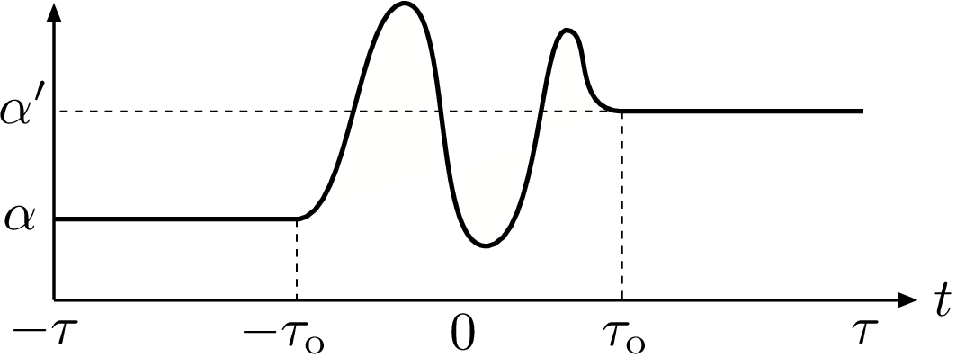
We assume that there is a set of parameters α\alpha which characterizes the system. For concreteness we assume that α\alpha takes its values in a compact subset of ℝn\mathbb{R}^{n} for some n>1n>1. Fix an arbitrary time scale τo>0\tau_{\mathrm{o}}>0. During the time interval [−τo,τo][-\tau_{\mathrm{o}},\tau_{\mathrm{o}}], an external agent performs an operation to the system by controlling α\alpha according to a protocol (i.e., a function of time tt) α⁡(t)\alpha(t) (with t∈[−τo,τo]t\in[-\tau_{\mathrm{o}},\tau_{\mathrm{o}}]) which is fixed in advance. The function α⁡(t)\alpha(t) need not be continuous. We write the initial and the final values of the parameters as α=α⁡(−τo)\alpha=\alpha(-\tau_{\mathrm{o}}) and α′=α⁡(τo)\alpha^{\prime}=\alpha(\tau_{\mathrm{o}}), respectively. We also take τ\tau which is much larger than τo\tau_{\mathrm{o}}, and consider the time evolution of the system in the longer time interval [−τ,τ][-\tau,\tau]. We extend the protocol to the whole time interval by simply setting α⁡(t)=α\alpha(t)=\alpha for t∈[−τ,−τo]t\in[-\tau,-\tau_{\mathrm{o}}] and α⁡(t)=α′\alpha(t)=\alpha^{\prime} for t∈[τo,τ]t\in[\tau_{\mathrm{o}},\tau]. See Figure 4. We denote the whole protocol as α^=(α⁡(t))t∈[−τ,τ]{\hat{\alpha}}=(\alpha(t))_{{t\in[-\tau,\tau]}}. A special protocol in which α⁡(t)\alpha(t) takes a constant value α\alpha throughout [−τ,τ][-\tau,\tau] is denoted as (α)(\alpha).

Refer to caption
Figure 4: The protocol α^=(α⁡(t))t∈[−τ,τ]{\hat{\alpha}}=(\alpha(t))_{{t\in[-\tau,\tau]}}, which brings the model parameters from α\alpha to α′\alpha^{\prime}. The parameters α⁡(t)\alpha(t) stay constant in the initial and the final stages.

We consider a Markov jump process characterized by a protocol α^{\hat{\alpha}}.

For given parameters α\alpha and x,y∈𝒮x,y\in{\cal S} such that x≠yx\neq y, let Rx→yα≥0R^{\alpha}_{x\to y}\geq 0 be the transition rate from the state xx to yy. Physically speaking transitions in our system is caused by interactions between the system and heat baths attached to it. We assume that Rx→yα≠0R^{\alpha}_{x\to y}\neq 0 implies Ry→xα≠0R^{\alpha}_{y\to x}\neq 0 for any x≠yx\neq y. We also assume that the whole state space 𝒮{\cal S} is “connected” by nonvanishing Rx→yαR^{\alpha}_{x\to y}. More precisely, for any x,y∈𝒮x,y\in{\cal S} with x≠yx\neq y, one can take a sequence x0,x1,…,xnx_{0},x_{1},\ldots,x_{n} such that x0=xx_{0}=x, xn=yx_{n}=y, and Rxj−1→xjα≠0R^{\alpha}_{x_{j-1}\to x_{j}}\neq 0 for any j=1,2,…,nj=1,2,\ldots,n. We also define the escape rate at x∈𝒮x\in{\cal S} by

λxα:=∑y∈𝒮(y≠x)Rx→yα.\lambda^{\alpha}_{x}:=\mathop{\sum_{y\in{\cal S}}}_{(y\neq x)}R^{\alpha}_{x\to y}. (2.1)

The Markov jump process corresponding to the protocol α^=(α⁡(t))t∈[−τ,τ]{\hat{\alpha}}=(\alpha(t))_{t\in[-\tau,\tau]} is defined by the master equation

d​px​(t)d​t=−λxα⁡(t)​px​(t)+∑y∈𝒮(y≠x)py​(t)​Ry→xα⁡(t),\dfrac{dp_{x}(t)}{dt}=-\lambda^{\alpha(t)}_{x}\,p_{x}(t)+\mathop{\sum_{y\in{\cal S}}}_{(y\neq x)}p_{y}(t)\,R^{\alpha(t)}_{y\to x}, (2.2)

for any x∈𝒮x\in{\cal S} and t∈[−τ,τ]{t\in[-\tau,\tau]}, where px​(t)p_{x}(t) is the probability to find the system in xx at time tt. The equation (2.2) is neatly rewritten in the vector notation as

d​𝒑​(t)d​t=𝖱α⁡(t)​𝒑​(t),\dfrac{d\boldsymbol{p}(t)}{dt}=\mathsf{R}^{\alpha(t)}\boldsymbol{p}(t), (2.3)

where 𝒑⁡(t)=(px​(t))x∈𝒮\boldsymbol{p}(t)=(p_{x}(t))_{x\in{\cal S}} is regarded as a column vector. The transition rate matrix77 7 The standard generator of a stochastic process is given by the transpose of 𝖱\mathsf{R}. 𝖱α\mathsf{R}^{\alpha} is defined by specifying its entries as (𝖱α)y​x=Rx→yα(\mathsf{R}^{\alpha})_{yx}=R^{\alpha}_{x\to y} for x≠yx\neq y and (𝖱α)x​x=−λxα(\mathsf{R}^{\alpha})_{xx}=-\lambda^{\alpha}_{x}. The formal solution of (2.3) is written as

𝒑⁡(t)=exp←⁡[∫−τtd​s​𝖱α⁡(s)]​𝒑init,\boldsymbol{p}(t)=\exp_{\leftarrow}\Bigl[\int_{-\tau}^{t}ds\,\mathsf{R}^{\alpha(s)}\Bigr]\,\boldsymbol{p}^{\mathrm{init}}, (2.4)

where 𝒑init\boldsymbol{p}^{\mathrm{init}} is the initial distribution given at −τ-\tau. The time-ordered exponential is defined by

exp←⁡[∫−τtd​s​𝖱α⁡(s)]\displaystyle\exp_{\leftarrow}\Bigl[\int_{-\tau}^{t}ds\,\mathsf{R}^{\alpha(s)}\Bigr]
:=limN↑∞exp[(t+τ)​𝖱α⁡(sN−1)N]exp[(t+τ)​𝖱α⁡(sN−2)N]⋯exp[(t+τ)​𝖱α⁡(s0)N],\displaystyle\ \ :=\lim_{N\uparrow\infty}\exp\Bigl[\frac{(t+\tau)\mathsf{R}^{\alpha(s_{N-1})}}{N}\Bigr]\exp\Bigl[\frac{(t+\tau)\mathsf{R}^{\alpha(s_{N-2})}}{N}\Bigr]\,\cdots\,\,\exp\Bigl[\frac{(t+\tau)\mathsf{R}^{\alpha(s_{0})}}{N}\Bigr], (2.5)

with sj={(t+τ)/N}​j−τs_{j}=\{(t+\tau)/N\}j-\tau. When α⁡(t)\alpha(t) is time-independent, (2.5) coincides with the usual exponential exp⁡[(t+τ)​𝖱α]\exp[(t+\tau)\mathsf{R}^{\alpha}].

It is a well known consequence of the Perron-Frobenius theorem that, for any parameter α\alpha, one has

lims↑∞exp⁡[s​𝖱α]​𝒑init=𝝆α,\lim_{s\uparrow\infty}\exp[s\,\mathsf{R}^{\alpha}]\,\boldsymbol{p}^{\mathrm{init}}=\boldsymbol{\rho}^{\alpha}, (2.6)

where 𝒑init\boldsymbol{p}^{\mathrm{init}} is an arbitrary initial probability distribution. Here 𝝆α=(ρxα)x∈𝒮\boldsymbol{\rho}^{\alpha}=(\rho^{\alpha}_{x})_{x\in{\cal S}} is the unique stationary probability distribution characterized by the condition 𝖱α​𝝆α=0\mathsf{R}^{\alpha}\boldsymbol{\rho}^{\alpha}=0. It is also known that ρxα>0\rho^{\alpha}_{x}>0 for any xx. Physically speaking 𝝆α\boldsymbol{\rho}^{\alpha} is the probability distribution for the nonequilibrium steady state (NESS) of the system with constant parameters α\alpha.

2.2 Description in terms of paths

It is sometimes more convenient to describe the Markov jump process in terms of a path (or a history) x^\hat{x} of the state. A path is naturally identified with a piecewise constant function x^=(x⁡(t))t∈[−τ,τ]\hat{x}=(x(t))_{{t\in[-\tau,\tau]}}, but we shall often specify it in terms of the history of jumps as

x^=(n,(x0,x1,…,xn),(t1,t2,…,tn)),\hat{x}=(n,(x_{0},x_{1},\ldots,x_{n}),(t_{1},t_{2},\ldots,t_{n})), (2.7)

where n=0,1,2,…n=0,1,2,\ldots is the total number of jumps, x0,…,xn∈𝒮x_{0},\ldots,x_{n}\in{\cal S} (such that xj−1≠xjx_{j-1}\neq x_{j} for j=1,…,nj=1,\ldots,n) are the states that the system has visited, and tjt_{j} is the time at which the jump xj−1→xjx_{j-1}\to x_{j} took place. They are ordered as −τ<t1<t2<…<tn<τ-\tau<t_{1}<t_{2}<\ldots<t_{n}<\tau, and we often write t0=−τt_{0}=-\tau and tn+1=τt_{n+1}=\tau. We also write x0x_{0} and xnx_{n} as x⁡(−τ)x(-\tau) and x⁡(τ)x(\tau), respectively. See Figure 5.

Refer to caption
Figure 5: A schematic picture of a path x^\hat{x}.

Then the weight (more precisely, the transition probability density) associated with a path x^\hat{x} is

𝒯α^[x^]:=∏j=1nRxj−1→xjα⁡(tj)∏j=0nexp[−∫tjtj+1dtλxjα⁡(t)].{\cal T}^{{\hat{\alpha}}}[\hat{x}]:=\prod_{j=1}^{n}R^{\alpha(t_{j})}_{x_{j-1}\to x_{j}}\,\prod_{j=0}^{n}\exp\Bigl[-\int_{t_{j}}^{t_{j+1}}dt\,\lambda_{x_{j}}^{\alpha(t)}\Bigr]. (2.8)

The weight is normalized so that

∫𝒟​x^​δx⁡(−τ),x​𝒯α^​[x^]=1\int{\cal D}\hat{x}\,\delta_{x(-\tau),x}\,{\cal T}^{{\hat{\alpha}}}[\hat{x}]=1 (2.9)

for any initial state x∈𝒮x\in{\cal S}, where the “integral” over all the paths is defined by

∫𝒟x^(⋯):=∑n=0∞∑x0,…,xn∈𝒮(xj−1≠xj)∫−ττdt1∫t1τdt2∫t2τdt3⋯∫tn−1τdtn(⋯).\int{\cal D}\hat{x}(\cdots):=\sum_{n=0}^{\infty}\ \mathop{\sum_{x_{0},\ldots,x_{n}\in{\cal S}}}_{(x_{j-1}\neq x_{j})}\ \int_{-\tau}^{\tau}dt_{1}\int_{{t_{1}}}^{\tau}dt_{2}\int_{{t_{2}}}^{\tau}dt_{3}\cdots\int_{{t_{n-1}}}^{\tau}dt_{n}(\cdots). (2.10)

In this language, the general solution (2.4) is written as

px​(t)=∫𝒟​x^​px⁡(−τ)init​δx⁡(t),x​𝒯α^​[x^].p_{x}(t)=\int{\cal D}\hat{x}\,p_{x(-\tau)}^{\mathrm{init}}\,\delta_{x(t),x}\,{\cal T}^{{\hat{\alpha}}}[\hat{x}]. (2.11)

One way to see the equivalence of (2.4) and (2.11) is to write the matrix product explicitly (in terms of the sums over 𝒮{\cal S}) in (2.5).

Let f⁡[x^]f[\hat{x}] be an arbitrary function of x^\hat{x}. We define the expectation value of f⁡[x^]f[\hat{x}] by

⟨f⟩st→α^:=∫𝒟​x^​f​[x^]​ρx⁡(−τ)α⁡(−τ)​𝒯α^​[x^],\langle f\rangle^{{\hat{\alpha}}}_{\mathrm{st}\to}:=\int{\cal D}\hat{x}\,f[\hat{x}]\,\rho^{\alpha(-\tau)}_{x(-\tau)}\,{\cal T}^{{\hat{\alpha}}}[\hat{x}], (2.12)

where the subscript “st→\mathrm{st}\to” indicates that the system starts from the steady state for parameter α⁡(−τ)\alpha(-\tau), and nothing is specified for the final condition. We stress that this is a physically natural expectation, which can be realized experimentally.

2.3 Entropy production, work, and time-reversal

Let us further specify our problem, and also introduce some important quantities.

We assume that each state x∈𝒮x\in{\cal S} is associated with its energy Hxν∈ℝH^{\nu}_{x}\in\mathbb{R}. Here ν\nu is a parameter (or a set of parameters) that characterizes the Hamiltonian HxνH^{\nu}_{x}, and is a component of α\alpha. See (2.30) and (2.34) for examples. We assume that ν\nu takes its value in a compact subset of ℝn′\mathbb{R}^{n^{\prime}} for some n′≥1n^{\prime}\geq 1.

Entropy production:

For any x,y∈𝒮x,y\in{\cal S} such that Rx→yα≠0R^{\alpha}_{x\to y}\neq 0, we define the entropy production in the heat baths88 8 Throughout the present paper, the entropy production always means the entropy production in the heat baths. associated with the transition x→y{x\to y} by

θx→yα:=log⁡Rx→yαRy→xα,\theta^{\alpha}_{x\to y}:=\log\frac{R^{\alpha}_{x\to y}}{R^{\alpha}_{y\to x}}, (2.13)

or, equivalently, by the “local detailed balance condition”

Ry→xα=e−θx→yα​Rx→yα.R^{\alpha}_{y\to x}=e^{-\theta^{\alpha}_{x\to y}}\,R^{\alpha}_{x\to y}. (2.14)

Clearly one has θx→yα=−θy→xα\theta^{\alpha}_{x\to y}=-\theta^{\alpha}_{y\to x}. Mathematically speaking (2.13) is a mere definition. With this definition of θx→yα\theta^{\alpha}_{x\to y}, we can justifies the “detailed fluctuation theorem” (6.4), which will be a basis of the present work. To give the quantity a physical interpretation as entropy production, we need some preparations.

A class of processes called equilibrium (stochastic) dynamics describe a system attached to heat baths with a single temperature and free from any non-conservative forces (see footnote 15). Such a system approaches the corresponding equilibrium state after a sufficiently long time99 9 The approach to equilibrium is indeed a nonequilibrium phenomenon that can be studied in the framework of equilibrium dynamics. . The transition rates Rx→y(β,ν)R^{(\beta,\nu)}_{x\to y} (where we have written α=(β,ν)\alpha={(\beta,\nu)}) in an equilibrium dynamics satisfy the detailed balance condition

e−β​Hxν​Rx→y(β,ν)=e−β​Hyν​Ry→x(β,ν),e^{-\beta H^{\nu}_{x}}R^{(\beta,\nu)}_{x\to y}=e^{-\beta H^{\nu}_{y}}R^{(\beta,\nu)}_{y\to x}, (2.15)

for any x,y∈𝒮x,y\in{\cal S}. Here β\beta is the single inverse temperature of the heat baths. It is well known (and easy to prove) that the condition (2.15) ensures that the corresponding stationary distribution is the canonical distribution ρx(β,ν)=e−β​Hxν/Zν​(β)\rho^{(\beta,\nu)}_{x}=e^{-\beta H^{\nu}_{x}}/Z_{\nu}(\beta), where Zν​(β)=∑x∈𝒮e−β​HxνZ_{\nu}(\beta)=\sum_{x\in{\cal S}}e^{-\beta H^{\nu}_{x}} is the normalization constant.

Under the detailed balance condition (2.15), the entropy production (2.13) becomes

θx→y(β,ν)=β⁡(Hxν−Hyν)=−β​qx→y,\theta^{(\beta,\nu)}_{x\to y}=\beta\,(H^{\nu}_{x}-H^{\nu}_{y})=-\beta\,q_{x\to y}, (2.16)

where qx→y=Hyν−Hxνq_{x\to y}=H^{\nu}_{y}-H^{\nu}_{x} is the change in the energy of the system, which is equal to the heat transferred from the baths to the system. The final expression in (2.16) is nothing but the well-known formula for the change (or the production) of entropy in equilibrium thermodynamics.

The main subject of the present work is non-equilibrium stochastic dynamics, for which the detailed balance condition (2.15) can never be satisfied for any choice of β\beta and HxνH^{\nu}_{x}. We nevertheless assume here that the entropy production θx→yα\theta^{\alpha}_{x\to y} is written as

θx→yα=−βB​qx→y,\theta^{\alpha}_{x\to y}=-\beta_{\mathrm{B}}\,q_{x\to y}, (2.17)

where βB\beta_{\mathrm{B}} is the inverse temperature of the single heat bath1010 10 We assume here (and in what follows) that each transition is associated with only a single bath. See also section 2.4. that is relevant to the transition x→y{x\to y}, and qx→yq_{x\to y} is the energy (heat) transferred from the bath to the system during the transition. The idea behind the identification (2.17) is that heat baths are always in equilibrium states so that we can use the relation from equilibrium thermodynamics for each transition, even when the system never settles to equilibrium1111 11 In a formulations based on a stochastic process (as in the present work), the relation (2.17) is nothing more than an interpretation. In more microscopic formulations based on mechanics, one may justify such relations. See, e.g., [43]. .

Throughout the present work we assume that the nonequilibrium system can be interpreted as a perturbation to an equilibrium system. As for the entropy production we write

θx→yα=ψx→yα+β⁡(Hxν−Hyν),\theta^{\alpha}_{x\to y}=\psi^{\alpha}_{x\to y}+\beta\,(H^{\nu}_{x}-H^{\nu}_{y}), (2.18)

where β>0\beta>0 is a certain reference inverse temperature, which may not be unique. The quantity ψx→yα\psi^{\alpha}_{x\to y} should be called the nonequilibrium part of entropy production. It also satisfies ψx→yα=−ψy→xα\psi^{\alpha}_{x\to y}=-\psi^{\alpha}_{y\to x}.

For a given path x^\hat{x} as in (2.7), we can define the total entropy production in x^\hat{x} as

Θα^​[x^]=∑j=1nθxj−1→xjα⁡(tj),\Theta^{{\hat{\alpha}}}[\hat{x}]=\sum_{j=1}^{n}{\theta}^{\alpha(t_{j})}_{x_{j-1}\to x_{j}}, (2.19)

and its nonequilibrium part as

Ψα^​[x^]=∑j=1nψxj−1→xjα⁡(tj).\Psi^{{\hat{\alpha}}}[\hat{x}]=\sum_{j=1}^{n}{\psi}^{\alpha(t_{j})}_{x_{j-1}\to x_{j}}. (2.20)

For any subinterval [τ1,τ2]⊂[−τ,τ][\tau_{1},\tau_{2}]\subset[-\tau,\tau], we define partial entropy productions by

Θ[τ1,τ2],α^[x^]=∑j=1nχ[tj∈[τ1,τ2]]θxj−1→xjα⁡(tj),\displaystyle\Theta^{[\tau_{1},\tau_{2}],{\hat{\alpha}}}[\hat{x}]=\sum_{j=1}^{n}\chi\bigl[t_{j}\in[\tau_{1},\tau_{2}]\bigr]\,{\theta}^{\alpha(t_{j})}_{x_{j-1}\to x_{j}}, (2.21)
Ψ[τ1,τ2],α^[x^]=∑j=1nχ[tj∈[τ1,τ2]]ψxj−1→xjα⁡(tj),\displaystyle\Psi^{[\tau_{1},\tau_{2}],{\hat{\alpha}}}[\hat{x}]=\sum_{j=1}^{n}\chi\bigl[t_{j}\in[\tau_{1},\tau_{2}]\bigr]\,{\psi}^{\alpha(t_{j})}_{x_{j-1}\to x_{j}}, (2.22)

where χ⁡[true]=1\chi[\text{true}]=1 and χ⁡[false]=0\chi[\text{false}]=0.

Work:

Let us write the protocol for the parameter of the Hamiltonian as ν^:=(ν⁡(t))t∈[−τ,τ]{\hat{\nu}}:=(\nu(t))_{{t\in[-\tau,\tau]}}, which is a component of the full protocol α^{\hat{\alpha}}. For a path x^\hat{x}, we define

Wν^​[x^]:=∑j=0n(Hxjν⁡(tj+1)−Hxjν⁡(tj))=∑j=0n∫tjtj+1d​t​d​ν​(t)d​t​[∂Hx⁡(t)ν∂ν]ν=ν⁡(t),W^{\hat{\nu}}[\hat{x}]:=\sum_{j=0}^{n}(H^{\nu(t_{j+1})}_{x_{j}}-H^{\nu(t_{j})}_{x_{j}})=\sum_{j=0}^{n}\int_{t_{j}}^{t_{j+1}}dt\,\dfrac{d\nu(t)}{dt}\left[\dfrac{\partial H_{x(t)}^{\nu}}{\partial\nu}\right]_{\nu=\nu(t)}, (2.23)

where the final expression is valid only when ν⁡(t)\nu(t) is differentiable. Note that Hxjν⁡(tj+1)−Hxjν⁡(tj)H^{\nu(t_{j+1})}_{x_{j}}-H^{\nu(t_{j})}_{x_{j}} is the change in the energy of the system during the interval (tj,tj+1)(t_{j},t_{j+1}), in which the state of the system is always xjx_{j}. Since this change in the energy is caused solely by the change in ν\nu, we can identify it with the work done by the external agent who operates on the system. Therefore (2.23) is the total work done by the external agent to the system in the path x^\hat{x}. Note that, since ν⁡(t)\nu(t) varies only for t∈[−τo,τo]t\in[-\tau_{\mathrm{o}},\tau_{\mathrm{o}}], the summand in (2.23) vanishes if (tj,tj+1)∩[−τo,τo]=∅(t_{j},t_{j+1})\cap[-\tau_{\mathrm{o}},\tau_{\mathrm{o}}]=\emptyset.

It is obvious from (2.18) that Θ\Theta, Ψ\Psi, and WW are related with each other. In fact by summing up (2.18) for all the transitions in x^\hat{x}, we see

Θα^​[x^]\displaystyle\Theta^{{\hat{\alpha}}}[\hat{x}] =Ψα^​[x^]+β​∑j=1n(Hxj−1ν⁡(tj)−Hxjν⁡(tj))\displaystyle=\Psi^{{\hat{\alpha}}}[\hat{x}]+\beta\sum_{j=1}^{n}\bigl(H^{\nu(t_{j})}_{x_{j-1}}-H^{\nu(t_{j})}_{x_{j}}\bigr)
=Ψα^​[x^]+β⁡{∑j=0n(Hxjν⁡(tj+1)−Hxjν⁡(tj))−Hxnν⁡(tn+1)+Hx0ν⁡(t0)}\displaystyle=\Psi^{{\hat{\alpha}}}[\hat{x}]+\beta\Bigl\{\sum_{j=0}^{n}\bigl(H^{\nu(t_{j+1})}_{x_{j}}-H^{\nu(t_{j})}_{x_{j}}\bigr)-H_{x_{n}}^{\nu(t_{n+1})}+H_{x_{0}}^{\nu(t_{0})}\Bigr\}
=Ψα^​[x^]+β​Wν^​[x^]+β⁡(Hx⁡(−τ)ν⁡(−τ)−Hx⁡(τ)ν⁡(τ)).\displaystyle=\Psi^{{\hat{\alpha}}}[\hat{x}]+\beta\,W^{\hat{\nu}}[\hat{x}]+\beta\bigl(H^{\nu(-\tau)}_{x(-\tau)}-H^{\nu(\tau)}_{x(\tau)}\Bigr). (2.24)

Time-reversal:

For a path x^\hat{x} as in (2.7), we define its time-reversal x^†\hat{x}^{\dagger} as

x^†=(n,(xn,xn−1,…,x0),(−tn,−tn−1,…,−t2,−t1)).\hat{x}^{\dagger}=(n,(x_{n},x_{n-1},\ldots,x_{0}),(-t_{n},-t_{n-1},\ldots,-t_{2},-t_{1})). (2.25)

If we use the language of function and denote original path as x^=(x⁡(t))t∈[−τ,τ]\hat{x}=(x(t))_{{t\in[-\tau,\tau]}}, the time-reversed path is x^†=(x⁡(−t))t∈[−τ,τ]\hat{x}^{\dagger}=(x(-t))_{{t\in[-\tau,\tau]}}. Similarly for a protocol α^=(α⁡(t))t∈[−τ,τ]{\hat{\alpha}}=(\alpha(t))_{{t\in[-\tau,\tau]}} and its component ν^=(ν⁡(t))t∈[−τ,τ]{\hat{\nu}}=(\nu(t))_{t\in[-\tau,\tau]}, we define their time-reversal as α^†=(α⁡(−t))t∈[−τ,τ]{\hat{\alpha}^{\dagger}}=(\alpha(-t))_{{t\in[-\tau,\tau]}} and ν^=(ν⁡(−t))t∈[−τ,τ]{\hat{\nu}}=(\nu(-t))_{{t\in[-\tau,\tau]}}, respectively.

One easily finds that the total entropy production, its nonequilibrium part, and the work are antisymmetric with respect to the time-reversal, i.e.,

Θα^​[x^]=−Θα^†​[x^†],Ψα^​[x^]=−Ψα^†​[x^†],Wν^​[x^]=−Wν^†​[x^†].\Theta^{{\hat{\alpha}}}[\hat{x}]=-\Theta^{{\hat{\alpha}^{\dagger}}}[\hat{x}^{\dagger}],\quad\Psi^{{\hat{\alpha}}}[\hat{x}]=-\Psi^{{\hat{\alpha}^{\dagger}}}[\hat{x}^{\dagger}],\quad W^{\hat{\nu}}[\hat{x}]=-W^{{\hat{\nu}^{\dagger}}}[\hat{x}^{\dagger}]. (2.26)

Measurability of the quantities:

In operational approaches to thermodynamics we believe it essential to distinguish between physical quantities which are experimentally measurable (at least in principle) and which are not. In what follows we assume that a path x^\hat{x} has been realized, and ask whether the quantities Wν^​[x^]W^{\hat{\nu}}[\hat{x}], Θα^​[x^]\Theta^{{\hat{\alpha}}}[\hat{x}], and Ψα^​[x^]\Psi^{{\hat{\alpha}}}[\hat{x}] are measurable. This corresponds to the measurability of these quantities in a single experiment.

As in most treatments of equilibrium thermodynamics, we assume that the total work Wν^​[x^]W^{\hat{\nu}}[\hat{x}] is measurable. The work is a purely mechanical quantity, and the external agent can, in principle, always determine it by precisely measuring the (generalized) force and the displacement.

We next argue that the total entropy production (in the baths) Θα^​[x^]\Theta^{{\hat{\alpha}}}[\hat{x}] is also measurable. Suppose that the system is in touch with nn heat baths, where the inverse temperature of the jj-th bath is βj\beta_{j}. Let Qjα^​[x^]Q_{j}^{{\hat{\alpha}}}[\hat{x}] be the total amount of heat that flowed into the system from the jj-th bath during the experiment, i.e., the sum of qx→yq_{x\to y} for every transition (which involve the jj-th bath) in the path x^\hat{x} . We assume that the total heat Qjα^​[x^]Q_{j}^{{\hat{\alpha}}}[\hat{x}] can be measured for each jj. This may not be a trivial assumption, but in principle we can think of carefully designed heat baths where heat flux can be monitored accurately1212 12 Such measurements are indeed possible in modern calorimetry. . Since the relation (2.17) means that the total entropy production is written as Θα^[x^]=−∑j=1nβjQjα^[x^]\Theta^{{\hat{\alpha}}}[\hat{x}]=-\sum_{j=1}^{n}\beta_{j}Q_{j}^{{\hat{\alpha}}}[\hat{x}], we conclude that Θα^​[x^]\Theta^{{\hat{\alpha}}}[\hat{x}] is measurable.

The measurability of the nonequilibrium part Ψα^​[x^]\Psi^{{\hat{\alpha}}}[\hat{x}] of the total entropy production is more subtle. We argue that Ψα^​[x^]\Psi^{{\hat{\alpha}}}[\hat{x}] is measurable or semi-measurable depending on the model. (See the next section for details of the models.) In the models for heat conduction, where the system exchanges energy only with heat baths, we find Ψα^[x^]=−∑j=1n(βj−β)Qjα^[x^]\Psi^{{\hat{\alpha}}}[\hat{x}]=-\sum_{j=1}^{n}(\beta_{j}-\beta)Q_{j}^{{\hat{\alpha}}}[\hat{x}] from (2.33). This means that Ψα^​[x^]\Psi^{{\hat{\alpha}}}[\hat{x}] is determined from the measurable total heat Qjα^​[x^]Q_{j}^{{\hat{\alpha}}}[\hat{x}]. In the models of systems driven by an external non-conservative force, on the other hand, the system exchanges energy with the external field as well as the heat baths. It then turns out (see (2.36)) that Ψα^​[x^]\Psi^{{\hat{\alpha}}}[\hat{x}] is identical to β\beta times the total work done to the system by the external field. The work done by the external field may be measured in principle1313 13 One strategy is to measure the back action from the system to the generator (such as a coil) of the field. In a colloidal system it may be possible to determine the work done by the field by precisely measuring the positions of charged particles. , but the measurement seems to be extremely difficult in general. We thus regard Ψα^​[x^]\Psi^{{\hat{\alpha}}}[\hat{x}] as a semi-measurable quantity in this case.

2.4 Examples

Although our theory applies to a large variety of physical models, it might be useful to have some concrete examples in mind. Here we define a standard class of equilibrium dynamics, and then describe two typical problems of nonequilibrium physics.

Equilibrium dynamics:

Before discussing nonequilibrium problems, let us discuss equilibrium dynamics, which will be the starting point.

To define transition rates, it is convenient to first specify the Hamiltonian HxνH^{\nu}_{x} and the connectivity function c⁡(x,y)c(x,y) such that c⁡(x,y)=c⁡(y,x)≥0c(x,y)=c(y,x)\geq 0 for any x,y∈𝒮x,y\in{\cal S} with x≠yx\neq y. We assume that the state space 𝒮{\cal S} is connected via nonvanishing c⁡(x,y)c(x,y), or more precisely, for any x,y∈𝒮x,y\in{\cal S} one can take a sequence x0,x1,…,xnx_{0},x_{1},\ldots,x_{n} such that x0=xx_{0}=x, xn=yx_{n}=y, and c⁡(xj−1,xj)≠0c(x_{j-1},x_{j})\neq 0 for any j=1,2,…,nj=1,2,\ldots,n. We make no assumptions on the Hamiltonian HxνH^{\nu}_{x} except that it is real.

Then the transition rates for the equilibrium dynamics at the inverse temperature β\beta may be defined, for example, as

Rx→y(β,ν)=c⁡(x,y)​eβ​Hxν,R^{(\beta,\nu)}_{x\to y}=c(x,y)\,e^{\beta H^{\nu}_{x}}, (2.27)

or

Rx→y(β,ν)=c⁡(x,y)​e(β/2)​(Hxν−Hyν).R^{(\beta,\nu)}_{x\to y}=c(x,y)\,e^{(\beta/2)(H^{\nu}_{x}-H^{\nu}_{y})}. (2.28)

It is clear that both the definitions satisfy the necessary conditions for transition rates including the detailed balance condition (2.15).

Suppose that one has Hxν=HyνH^{\nu}_{x}=H^{\nu}_{y} and c⁡(x,y)≠0c(x,y)\neq 0 for some x≠yx\neq y. Then the rate (2.28) becomes Rx→y(β,ν)=Ry→x(β,ν)=c⁡(x,y)R^{(\beta,\nu)}_{x\to y}=R^{(\beta,\nu)}_{y\to x}=c(x,y), and is independent of the inverse temperature β\beta.

The abstract scheme discussed above applies to various concrete physical settings. Let us describe a system of particles on a lattice. Let the lattice Λ\Lambda be a finite set whose elements are denoted as u,v​…∈Λu,v\ldots\in\Lambda. We denote by ℬ{\cal B} the set of bonds on Λ\Lambda. More precisely the element of ℬ{\cal B} is a pair {u,v}={v,u}\{u,v\}=\{v,u\} with some u,v∈Λu,v\in\Lambda such that u≠vu\neq v. We assume that Λ\Lambda is connected via the bonds in ℬ{\cal B}. The simplest example is the one-dimensional periodic lattice Λ={1,2,…,L}\Lambda=\{1,2,\ldots,L\} with ℬ={{x,x+1}|x∈Λ}{\cal B}=\bigl\{\{x,x+1\}\,\bigr|\,x\in\Lambda\bigr\}, where we identify L+1L+1 with 11.

Refer to caption
Figure 6: A configuration x=(x1,x2,x3)x=(x_{1},x_{2},x_{3}) of three particles on the lattice.

We assume that there are NN particles on the lattice, and let xx denote a configuration of the particles on Λ\Lambda. More precisely, we set x=(x1,…,xN)x=(x_{1},\ldots,x_{N}), where xj∈Λx_{j}\in\Lambda is the position of the jj-th particle (j=1,…,Nj=1,\ldots,N). One may or may not impose the hard-core condition, i.e., xj≠xkx_{j}\neq x_{k} whenever j≠kj\neq k. See Figure 6.

For any two configurations x=(x1,…,xN)x=(x_{1},\ldots,x_{N}) and y=(y1,…,yN)y=(y_{1},\ldots,y_{N}), we set c⁡(x,y)=1c(x,y)=1 if {xk,yk}∈ℬ\{x_{k},y_{k}\}\in{\cal B} for some kk and xj=yjx_{j}=y_{j} for any jj such that j≠kj\neq k, and c⁡(x,y)=0c(x,y)=0 otherwise. In other words, c⁡(x,y)=1c(x,y)=1 if and only if one can modify the configuration xx into yy by moving one particle along a bond in ℬ{\cal B}.

As for the Hamiltonian, the standard choice is

Hx:=∑j=1NV1​(xj)+∑j,k=1(j>k)NV2​(xj,xk),H_{x}:=\sum_{j=1}^{N}V_{1}(x_{j})+\mathop{\sum_{j,k=1}}_{(j>k)}^{N}V_{2}(x_{j},x_{k}), (2.29)

where the single particle potential V1​(⋅)V_{1}(\cdot) and the two-particle interaction potential V2​(⋅,⋅)V_{2}(\cdot,\cdot) are arbitrary real valued functions on Λ\Lambda and Λ×Λ\Lambda\times\Lambda, respectively.

Heat conduction:

Let us discuss an idealized model of heat conduction. We assume that the system interacts with nn heat baths with different temperatures. We label the baths by the index j=1,2,…,nj=1,2,\ldots,n, and denote by βj\beta_{j} the inverse temperature of the jj-th bath. The set of parameters that characterizes the model is

α=(β1,…,βn,ν).\alpha=(\beta_{1},\ldots,\beta_{n},\nu). (2.30)

With any x,y∈𝒮x,y\in{\cal S} such that c⁡(x,y)≠0c(x,y)\neq 0 we associate a unique index j⁡(x,y)=j⁡(y,x)∈{1,…,n}j(x,y)=j(y,x)\in\{1,\ldots,n\}, which indicates that the j⁡(x,y)j(x,y)-th bath is relevant for the transition between xx and yy. Then we define the transition rate as

Rx→yα=Rx→y(βj⁡(x,y),ν),R^{\alpha}_{{x\to y}}=R^{(\beta_{j(x,y)},\nu)}_{{x\to y}}, (2.31)

for any x,y∈𝒮x,y\in{\cal S} such that x≠yx\neq y, where the right-hand side is defined by (2.27) or (2.28).

From the definition (2.13), one finds

θx→yα=βj⁡(x,y)​(Hxν−Hyν)=Δ​βj⁡(x,y)​(Hxν−Hyν)+β⁡(Hxν−Hyν),\theta_{{x\to y}}^{\alpha}=\beta_{j(x,y)}\,(H^{\nu}_{x}-H^{\nu}_{y})=\mathit{\Delta}\beta_{j(x,y)}\,(H^{\nu}_{x}-H^{\nu}_{y})+\beta\,(H^{\nu}_{x}-H^{\nu}_{y}), (2.32)

where we have chosen the reference inverse temperature β\beta (somewhat arbitrarily), and wrote Δ​βj:=βj−β\mathit{\Delta}\beta_{j}:=\beta_{j}-\beta. Comparing with (2.18), one finds

ψx→yα=Δ​βj⁡(x,y)​(Hxν−Hyν),\psi^{\alpha}_{{x\to y}}=\mathit{\Delta}\beta_{j(x,y)}\,(H^{\nu}_{x}-H^{\nu}_{y}), (2.33)

which is indeed small when all the inverse temperatures β1,…,βn\beta_{1},\ldots,\beta_{n} are close to each other, and β\beta is chosen properly1414 14 In most of realistic situations for heat conduction, only some small portions of the system is in touch with the heat baths. To model such a situation by using a system of particles on a lattice, we assume that the energy of the system changes only when a particle hops within one of the portions which are in touch with the baths. In other words, if an allowed transition x→y{x\to y} is such that a particle hops outside the portions, then one must have Hxν=HyνH^{\nu}_{x}=H^{\nu}_{y}. We further use the transition rule (2.28) so as to make the corresponding transition rate (which is indeed 1) independent of any inverse temperatures. .

Driven system:

We shall illustrate a system which is in contact with a single heat bath with the inverse temperature β\beta, but is driven by a non-conservative external force.

For each pair x,y∈𝒮x,y\in{\cal S} such that c⁡(x,y)≠0c(x,y)\neq 0, we define a quantity dx→y∈ℝd_{{x\to y}}\in\mathbb{R} which satisfies the antisymmetry dx→y=−dy→xd_{{x\to y}}=-d_{y\to x}. Physically, dx→yd_{{x\to y}} is interpreted as the displacement (in the direction of the non-conservative external force) of the particle associated with the transition x→y{x\to y}. In the simplest example of particles on the one-dimensional periodic lattice, we set dx→y=1d_{{x\to y}}=1 if a particle jumps to the right in the transition x→y{x\to y}, and dx→y=−1d_{{x\to y}}=-1 if a particle jumps to the left.

We assume that the non-conservative1515 15 We define the force in this setting as fx→y=f​dx→yf_{{x\to y}}=fd_{x\to y}. The force fx→yf_{x\to y} is said to be conservative if one can write fx→y=Ux−Uyf_{{x\to y}}=U_{x}-U_{y} for any x,y∈𝒮x,y\in{\cal S} with a suitable function (i.e., potential) UxU_{x}. external force ff is applied to the system. The model is parameterized by

α=(β,ν,f).\alpha=(\beta,\nu,f). (2.34)

We then define the transition rate by

Rx→yα=eβ​f​dx→y/2​Rx→y(β,ν),R^{\alpha}_{x\to y}=e^{\beta fd_{x\to y}/2}\,R^{(\beta,\nu)}_{x\to y}, (2.35)

for any x,y∈𝒮x,y\in{\cal S} such that x≠yx\neq y, where the right-hand side is defined by (2.27) or (2.28).

From the definitions (2.13) and (2.18), one readily finds

ψx→yα=β​f​dx→y.\psi^{\alpha}_{{x\to y}}=\beta fd_{{x\to y}}. (2.36)

This means that the nonequilibrium part of the total entropy production Ψα^​[x^]\Psi^{\hat{\alpha}}[\hat{x}] (see (2.20)) can be interpreted as the total work done by the non-conservative external force to the system (multiplied by β\beta).

3 Jarzynski-type equalities for NESS

We start by presenting some exact equalities which are valid for general operations (i.e., protocols) to NESS. They are reminiscent of the Jarzynski equality (3.2), which holds for operations to equilibrium states [32, 30].

We note, however, that the derivation of these equalities for NESS is not as straightforward as that of the original Jarzynski equality [32]. One of the main difficulties is that we do not know the explicit form of the probability distribution 𝝆α\boldsymbol{\rho}^{\alpha} of NESS while the corresponding stationary distribution in the equilibrium case is the canonical distribution.

Our main equality is the following. We here consider a general protocol α^{\hat{\alpha}} introduced in the beginning of section 2.1. See, in particular, Figure 4. As we have discussed at the end of section 2.3, we regard that the work Wν^W^{\hat{\nu}} is measurable, and the nonequilibrium part Ψα^\Psi^{{\hat{\alpha}}} of the entropy production is measurable or semi-measurable depending on the model.

Theorem 3.1

There exists a function (that we call the free energy) F⁡(α)F(\alpha) of the parameters α\alpha which coincides with the equilibrium free energy −β−1log∑x∈𝒮e−β​Hxν-\beta^{-1}\log\sum_{x\in{\cal S}}e^{-\beta H^{\nu}_{x}} for an equilibrium system with α=(β,ν)\alpha=(\beta,\nu), and we have for any protocol α^{\hat{\alpha}} that

F(α′)−F(α)=−1βlimτ↑∞log⟨exp[−(βWν^+Ψα^)/2]⟩α^st→⟨exp[−(βWν^†+Ψα^†)/2]⟩α^†st→.F(\alpha^{\prime})-F(\alpha)=-\frac{1}{\beta}\lim_{\tau\uparrow\infty}\log\frac{\bigl\langle\,\exp[-(\beta\,W^{\hat{\nu}}+\Psi^{{\hat{\alpha}}})/2]\,\bigr\rangle^{{\hat{\alpha}}}_{\mathrm{st}\to}}{\bigl\langle\,\exp[-(\beta\,W^{{\hat{\nu}^{\dagger}}}+\Psi^{{\hat{\alpha}^{\dagger}}})/2]\,\bigr\rangle^{{\hat{\alpha}^{\dagger}}}_{\mathrm{st}\to}}. (3.1)

This theorem will be proved in section 6.2, using the results from section 7.

We recall that ν\nu is a component of α\alpha (as in (2.30) and (2.34)), and likewise the protocol ν^=(ν⁡(t))t∈[−τ,τ]{\hat{\nu}}=(\nu(t))_{t\in[-\tau,\tau]} is a component of the full protocol α^=(α⁡(t))t∈[−τ,τ]{\hat{\alpha}}=(\alpha(t))_{t\in[-\tau,\tau]}. Note that we fix the operation time scale τo\tau_{\mathrm{o}} when taking the limit τ↑∞\tau\uparrow\infty. It means that we are treating an arbitrary operation, including very “wild” ones.

The equality (3.1) expresses the difference of the (nonequilibrium) free energy in terms of the expectation values defined for nonequilibrium processes. In this sense it may be regarded as a nonequilibrium version of the Jarzynski equality

F⁡(β,ν′)−F⁡(β,ν)=−1β​log⁡⟨e−β​Wν^⟩eq→(β,ν^)F(\beta,\nu^{\prime})-F(\beta,\nu)=-\frac{1}{\beta}\log\bigl\langle e^{-\beta W^{\hat{\nu}}}\bigr\rangle^{(\beta,{\hat{\nu}})}_{\mathrm{eq}\to} (3.2)

for equilibrium processes. A fundamental difference of our equality from the original equality is that we must consider the expectation values for both the original protocol α^{\hat{\alpha}} and its time-reversal α^†{\hat{\alpha}^{\dagger}}. Let us stress, however, that the expectation ⟨⋯⟩st→α^†\langle\cdots\rangle^{{\hat{\alpha}^{\dagger}}}_{\mathrm{st}\to} is not at all unphysical; one simply executes the operation according to the protocol α^†{\hat{\alpha}^{\dagger}}, and considers a natural time-evolution starting from the NESS corresponding to α′\alpha^{\prime}. Another difference is that here the expectation values involve the nonequilibrium part Ψ\Psi of the entropy production as well as the work WW.

We recall that one can prove the minimum work principle ⟨Wν^⟩eq→(β,ν^)≥F⁡(β,ν′)−F⁡(β,ν)\langle W^{\hat{\nu}}\rangle^{(\beta,{\hat{\nu}})}_{\mathrm{eq}\to}\geq F(\beta,\nu^{\prime})-F(\beta,\nu), which is a representation of the second law of thermodynamics (in the standard equilibrium thermodynamics), by simply applying the Jensen inequality to the Jarzynski equality (3.2). Unfortunately our equality (3.1) does not lead directly to any inequalities since the right-hand side is the ratio of the two expectation values.

Below in Theorem 3.2, we see another equality which better resembles the original Jarzynski equality (3.2). But our (3.1) is of considerable importance especially because it is intimately related to thermodynamic relations in NESS, as we shall discuss in section 4.

We note that various exact equalities which are valid for general stochastic processes (including ours) have been derived from the “detailed fluctuation theorem” in, e.g., [33, 34, 35]. Many similar equalities can be derived in the same manner. We believe that our equality (3.1) is essentially different from these equalities. While the equalities derivable with the methods in [33, 34, 35] contain quantities like log⁡ρxα\log\rho^{\alpha}_{x} which depend explicitly on the unknown stationary distribution 𝝆α\boldsymbol{\rho}^{\alpha}, our equality only contains WW and Ψ\Psi which are (semi-)measurable thermodynamic type quantities. The derivation of our new equality is based not only on the “detailed fluctuation theorem” but also on the new “splitting lemma” (Lemma 6.1) which allows us to treat a process whose initial distribution is 𝝆α\boldsymbol{\rho}^{\alpha} without using 𝝆α\boldsymbol{\rho}^{\alpha} explicitly.

It may be inspiring to rewrite the quantity inside the limit in (3.1) as

log⁡⟨e−βWν^/2⟩α^mod⟨e−βWν^†/2⟩α^†mod+log⁡⟨exp[−Ψα^/2]⟩α^st→⟨exp[−Ψα^†/2]⟩α^†st→,\log\frac{\langle e^{-\beta\,W^{\hat{\nu}}/2}\rangle^{\hat{\alpha}}_{\mathrm{mod}}}{\langle e^{-\beta\,W^{\hat{\nu}^{\dagger}}/2}\rangle^{\hat{\alpha}^{\dagger}}_{\mathrm{mod}}}+\log\frac{\bigl\langle\,\exp[-\Psi^{{\hat{\alpha}}}/2]\,\bigr\rangle^{{\hat{\alpha}}}_{\mathrm{st}\to}}{\bigl\langle\,\exp[-\Psi^{{\hat{\alpha}^{\dagger}}}/2]\,\bigr\rangle^{{\hat{\alpha}^{\dagger}}}_{\mathrm{st}\to}}, (3.3)

where we have defined the modified expectation by

⟨f⟩modα^:=⟨fexp[−Ψα^/2]⟩α^st→⟨exp[−Ψα^/2]⟩α^st→.\langle f\rangle^{\hat{\alpha}}_{\mathrm{mod}}:=\frac{\bigl\langle\,f\,\exp[-\Psi^{{\hat{\alpha}}}/2]\,\bigr\rangle^{{\hat{\alpha}}}_{\mathrm{st}\to}}{\bigl\langle\,\exp[-\Psi^{{\hat{\alpha}}}/2]\,\bigr\rangle^{{\hat{\alpha}}}_{\mathrm{st}\to}}. (3.4)

We note that the extra weight exp[−Ψα^[x^]/2]\exp[-\Psi^{{\hat{\alpha}}}[\hat{x}]/2] has an effect of canceling the nonequilibrium contribution ψx→yα\psi^{\alpha}_{x\to y} in the transition rates. This is in particular true for the example of driven system discussed in section 2.4. Compare the transition rate (2.35) with the formula (2.36) for ψx→yα\psi^{\alpha}_{x\to y}.

The physics described by the expectation ⟨⋯⟩modα^\langle\cdots\rangle^{\hat{\alpha}}_{\mathrm{mod}} is then expected to be close to that of equilibrium. But there still is considerable “nonequilibrium effect” coming from the escape rates λxα\lambda^{\alpha}_{x}, which are untouched in the modification (3.4). Possible essential roles played by the escape rates in nonequilibrium states have been emphasized by Maes and his collaborators [36, 37, 38]. In the expectation ⟨⋯⟩modα^\langle\cdots\rangle^{\hat{\alpha}}_{\mathrm{mod}}, nonequilibrium flows are cancelled and we can focus on the effects from the escape rates. We still do not know if this interpretation leads us to any new insights.

Remark 1:

The equality (3.1) is one of the series of equalities which can be proved in the similar manner. A general form includes an arbitrary constant κ∈ℝ\kappa\in\mathbb{R}, and is

F(α′)−F(α)=−1βlimτ↑∞log⟨exp⁡[−κ​β​Wν^−Ψα^/2]⟩st→α^⟨exp⁡[−(1−κ)​β​Wν^†−Ψα^†/2]⟩st→α^†.F(\alpha^{\prime})-F(\alpha)=-\frac{1}{\beta}\lim_{\tau\uparrow\infty}\log\frac{\bigl\langle\,\exp[-\kappa\,\beta\,W^{\hat{\nu}}-\Psi^{{\hat{\alpha}}}/2]\,\bigr\rangle^{{\hat{\alpha}}}_{\mathrm{st}\to}}{\bigl\langle\,\exp[-(1-\kappa)\,\beta\,W^{\hat{\nu}^{\dagger}}-\Psi^{{\hat{\alpha}^{\dagger}}}/2]\,\bigr\rangle^{{\hat{\alpha}^{\dagger}}}_{\mathrm{st}\to}}. (3.5)

Remark 2:

We can also prove the following exact equalities which involve the total entropy production Θ\Theta, rather than its nonequilibrium part Ψ\Psi. See the end of section 6.2 for the proof. There exists a function S~​(α)\tilde{S}(\alpha) of the parameters α\alpha, and we have for any protocol α^{\hat{\alpha}} that

S~​(α′)−S~​(α)=limτ↑∞log⁡⟨exp[−Θα^/2]⟩α^st→⟨exp[−Θα^†/2]⟩α^†st→.\tilde{S}(\alpha^{\prime})-\tilde{S}(\alpha)=\lim_{\tau\uparrow\infty}\log\frac{\bigl\langle\,\exp[-\Theta^{{\hat{\alpha}}}/2]\,\bigr\rangle^{{\hat{\alpha}}}_{\mathrm{st}\to}}{\bigl\langle\,\exp[-\Theta^{{\hat{\alpha}^{\dagger}}}/2]\,\bigr\rangle^{{\hat{\alpha}^{\dagger}}}_{\mathrm{st}\to}}. (3.6)

Although one may be tempted to identify S~​(α)\tilde{S}(\alpha) as nonequilibrium entropy, this interpretation may not be adequate. For parameters α\alpha which correspond to equilibrium, one finds that S~​(α)\tilde{S}(\alpha) is (similar to but) not the same as the equilibrium entropy. See (6.15).

Another exact Jarzynski-type equality for NESS was derived by one of us (N.N.) in [39]. Since we can prove this equality with the same machinery as the previous one, we shall briefly discuss it here.

For an arbitrary function f⁡[x^]f[\hat{x}] of x^\hat{x}, we define its Ψ\Psi-modified expectation as

⟨f⟩Ψ-modα^:=⟨fexp[−(Ψ[−τ,−τ/2],(α)+Ψ[τ/2,τ],(α′))/2]⟩α^st→⟨exp[−(Ψ[−τ,−τ/2],(α)+Ψ[τ/2,τ],(α′))/2]⟩α^st→,\langle f\rangle^{{\hat{\alpha}}}_{\text{$\Psi$-mod}}:=\frac{\bigl\langle\,f\,\exp[-(\Psi^{[-\tau,-\tau/2],(\alpha)}+\Psi^{[\tau/2,\tau],(\alpha^{\prime})})/2]\,\bigr\rangle^{{\hat{\alpha}}}_{\mathrm{st}\to}}{\bigl\langle\,\exp[-(\Psi^{[-\tau,-\tau/2],(\alpha)}+\Psi^{[\tau/2,\tau],(\alpha^{\prime})})/2]\,\bigr\rangle^{{\hat{\alpha}}}_{\mathrm{st}\to}}, (3.7)

where Ψ\Psi for restricted time intervals are defined in (2.22). We have replaced the protocols by (α)(\alpha) and (α′)(\alpha^{\prime}) in order to emphasize that α⁡(t)\alpha(t) is constant in these intervals (we here assume τ≥2​τo\tau\geq 2\tau_{\mathrm{o}}). This is similar to the modified expectation (3.4) introduced above, but now the modification factor presents only in the time intervals [−τ,−τ/2][-\tau,-\tau/2] and [τ/2,τ][\tau/2,\tau]. One can say that the system is in the modified nonequilibrium at the beginning and the end of the history, while it is in the full-fledged nonequilibrium in the middle. This hybrid allows one to prove the following strong result.

Theorem 3.2

Let F⁡(α)F(\alpha) be the nonequilibrium free energy introduced in Theorem 3.1. For any protocol α^{\hat{\alpha}}, one has

limτ↑∞⟨e−β​Wν^⟩st→α^=e−β⁡{F⁡(α′)−F⁡(α)}limτ↑∞⟨exp[−Ψ[−τ/2,τ/2],α^†]⟩Ψ-modα^†.\lim_{\tau\uparrow\infty}\langle e^{-\beta\,W^{\hat{\nu}}}\rangle^{{\hat{\alpha}}}_{\mathrm{st}\to}=e^{-\beta\{F(\alpha^{\prime})-F(\alpha)\}}\,\lim_{\tau\uparrow\infty}\bigl\langle\exp[-\Psi^{[-\tau/2,\tau/2],{\hat{\alpha}^{\dagger}}}]\bigr\rangle^{{\hat{\alpha}^{\dagger}}}_{\text{\rm$\Psi$-mod}}. (3.8)

This theorem will be proved in section 6.3, using the results from section 7.

It is remarkable that the left-hand side of (3.8) only includes the standard mechanical work Wν^W^{\hat{\nu}} and the physically natural average ⟨⋯⟩st→α^\langle\cdots\rangle^{{\hat{\alpha}}}_{\mathrm{st}\to}. Although the right-hand side is a little more complicated, it was shown in [39] that it can also be measured experimentally at least when the “degree of nonequilibrium” is small enough.

By using the Jensen inequality, one can show from (3.8) a “second law”

limτ↑∞⟨Wν^⟩st→α^≥F(α′)−F(α)−1βlimτ↑∞log⟨exp[−Ψ[−τ/2,τ/2],α^†]⟩Ψ-modα^†.\lim_{\tau\uparrow\infty}\langle W^{\hat{\nu}}\rangle^{{\hat{\alpha}}}_{\mathrm{st}\to}\geq F(\alpha^{\prime})-F(\alpha)-\frac{1}{\beta}\lim_{\tau\uparrow\infty}\log\bigl\langle\exp[-\Psi^{[-\tau/2,\tau/2],{\hat{\alpha}^{\dagger}}}]\bigr\rangle^{{\hat{\alpha}^{\dagger}}}_{\text{$\Psi$-mod}}. (3.9)

4 Thermodynamic relations for NESS

We shall observe here that our main equality (3.1) can be used to generate thermodynamic relations associated with operations that bring a NESS to a different NESS. The simplest and the most important is the extended Clausius relation (4.5), (4.6), and (4.10), which was derived in our earlier works [2, 3]. We concentrate on heuristic arguments in the present section, and discuss corresponding rigorous results in section 5.

4.1 Extended Clausius relation and entropy

Extended Clausius relation:

Here we shall concentrate on a situation where the system is close to equilibrium and the change in the parameters during the operation is small. It is then expected that the arguments of the two exponential functions in the right-hand side of the equality (3.1) are small, because ψx→yα\psi^{\alpha}_{x\to y} vanishes in an equilibrium system, and Wν^W^{\hat{\nu}} is small if the change of the Hamiltonian is small. By expanding in these quantities to the lowest order, we see that (3.1) yields

F⁡(α′)−F⁡(α)≃12​β​{⟨β​Wν^+Ψα^⟩α^−⟨β​Wν^†+Ψα^†⟩α^†},F(\alpha^{\prime})-F(\alpha)\simeq\frac{1}{2\beta}\Bigl\{\langle\beta\,W^{\hat{\nu}}+\Psi^{\hat{\alpha}}\rangle^{\hat{\alpha}}-\langle\beta\,W^{\hat{\nu}^{\dagger}}+\Psi^{\hat{\alpha}^{\dagger}}\rangle^{\hat{\alpha}^{\dagger}}\Bigr\}, (4.1)

where we have abbreviated ⟨⋯⟩st→α^\langle\cdots\rangle^{{\hat{\alpha}}}_{\mathrm{st}\to} as ⟨⋯⟩α^\langle\cdots\rangle^{{\hat{\alpha}}} for simplicity. We also assumed τ\tau is sufficiently large, and have omitted limτ↑∞\lim_{\tau\uparrow\infty}.

Although (4.1) may be interpreted as a thermodynamic relation, it is much better to rewrite it in terms of the total entropy production Θ\Theta. By substituting (2.24), this becomes

β⁡{F⁡(α′)−F⁡(α)}≃⟨Θα^⟩α^−⟨Θα^†⟩α^†2+β​⟨Hν′⟩stα′−β​⟨Hν⟩stα.\beta\,\{F(\alpha^{\prime})-F(\alpha)\}\simeq\frac{\langle\Theta^{\hat{\alpha}}\rangle^{\hat{\alpha}}-\langle\Theta^{\hat{\alpha}^{\dagger}}\rangle^{\hat{\alpha}^{\dagger}}}{2}+\beta\,\langle H^{\nu^{\prime}}\rangle^{\alpha^{\prime}}_{\mathrm{st}}-\beta\,\langle H^{\nu}\rangle^{\alpha}_{\mathrm{st}}. (4.2)

For an arbitrary function gxg_{x} on 𝒮{\cal S}, we have defined its expectation value in the steady state with α\alpha as

⟨g⟩stα:=∑x∈𝒮gx​ρxα.\langle g\rangle^{\alpha}_{\mathrm{st}}:=\sum_{x\in{\cal S}}g_{x}\,\rho^{\alpha}_{x}. (4.3)

If one introduces the nonequilibrium entropy through the “familiar” relation

S⁡(α):=β⁡{⟨Hν⟩stα−F⁡(α)},S(\alpha):=\beta\bigl\{\langle H^{\nu}\rangle^{\alpha}_{\mathrm{st}}-F(\alpha)\bigr\}, (4.4)

the relation (4.2) becomes

S⁡(α′)−S⁡(α)≃−⟨Θα^⟩α^−⟨Θα^†⟩α^†2,S(\alpha^{\prime})-S(\alpha)\simeq-\frac{\langle\Theta^{\hat{\alpha}}\rangle^{\hat{\alpha}}-\langle\Theta^{\hat{\alpha}^{\dagger}}\rangle^{\hat{\alpha}^{\dagger}}}{2}, (4.5)

which is the extended Clausius relation obtained in [2, 3]. This is essentially the same as (1.4) in the introduction. To be slightly more precise about the near equality, we can write the same relation as

S⁡(α′)−S⁡(α)=−⟨Θα^⟩α^−⟨Θα^†⟩α^†2+O⁡(ϵ2​δ)+O⁡(δ2),S(\alpha^{\prime})-S(\alpha)=-\frac{\langle\Theta^{\hat{\alpha}}\rangle^{\hat{\alpha}}-\langle\Theta^{\hat{\alpha}^{\dagger}}\rangle^{\hat{\alpha}^{\dagger}}}{2}+O(\epsilon^{2}\delta)+O(\delta^{2}), (4.6)

where ϵ\epsilon denotes the “degree of nonequilibrium”, and δ\delta denotes the amount of change in the parameters (see section 5 for precise definitions). The O⁡(δ2)O(\delta^{2}) term can be omitted for a quasi-static (i.e., smooth and slow) protocol. In Theorems 5.2 and 5.3, we present corresponding rigorous estimates.

Consider an equilibrium protocol α^eq=(αeq​(t))t∈[−τ,τ]{\hat{\alpha}}_{\mathrm{eq}}=(\alpha_{\mathrm{eq}}(t))_{t\in[-\tau,\tau]}, where αeq​(t)\alpha_{\mathrm{eq}}(t) for any t∈[−τ,τ]{t\in[-\tau,\tau]} corresponds to an equilibrium system. In such a case the standard adiabatic theorem implies that ⟨Θα^eq⟩α^eq≃−⟨Θα^eq†⟩α^eq†\langle\Theta^{{\hat{\alpha}}_{\mathrm{eq}}}\rangle^{{\hat{\alpha}}_{\mathrm{eq}}}\simeq-\langle\Theta^{{\hat{\alpha}}_{\mathrm{eq}}^{\dagger}}\rangle^{{\hat{\alpha}}_{\mathrm{eq}}^{\dagger}} for a sufficiently slow and smooth process. Then the relation (4.5) becomes

S⁡(αeq′)−S⁡(αeq)≃−⟨Θα^eq⟩α^eq,S(\alpha^{\prime}_{\mathrm{eq}})-S(\alpha_{\mathrm{eq}})\simeq-\langle\Theta^{{\hat{\alpha}}_{\mathrm{eq}}}\rangle^{{\hat{\alpha}}_{\mathrm{eq}}}, (4.7)

which is nothing but the standard Clausius relation (1.1). Since S⁡(αeq)S(\alpha_{\mathrm{eq}}) coincides with the standard entropy, we find the the extended Clausius relation (4.5) is an extension of the standard Clausius relation.

Note that, in a NESS, both ⟨Θα^⟩α^\langle\Theta^{\hat{\alpha}}\rangle^{\hat{\alpha}} and ⟨Θα^†⟩α^†\langle\Theta^{\hat{\alpha}^{\dagger}}\rangle^{\hat{\alpha}^{\dagger}} grow proportionally with the total time τ\tau since there always is a nonvanishing entropy production. The extended Clausius relation (4.5) shows that their difference is a finite quantity independent of τ\tau (provided that τ\tau is long enough) and characterizes the effect of the operation. It is crucial that the quantities ⟨Θα^⟩α^\langle\Theta^{\hat{\alpha}}\rangle^{\hat{\alpha}} and ⟨Θα^†⟩α^†\langle\Theta^{\hat{\alpha}^{\dagger}}\rangle^{\hat{\alpha}^{\dagger}} can be measured by executing (at least) two experiments with the protocol α^{\hat{\alpha}} and the corresponding reverse protocol α^†{\hat{\alpha}^{\dagger}}.

Excess entropy production:

The right-hand side of the extended Clausius relation (4.5) or (4.6) can also be written in terms of an interesting quantity called the excess entropy production. We first define the entropy production rate σstα\sigma_{\mathrm{st}}^{\alpha} in the NESS with the parameters α\alpha by

σstα:=12​τ​⟨Θ(α)⟩st→(α),\sigma_{\mathrm{st}}^{\alpha}:=\frac{1}{2\tau}\langle\Theta^{(\alpha)}\rangle^{(\alpha)}_{\mathrm{st}\to}, (4.8)

where (α){(\alpha)} denotes the protocol in which α⁡(t)=α\alpha(t)=\alpha for any t∈[−τ,τ]{t\in[-\tau,\tau]}. We shall prove in section 7.5 that the definition is independent of τ\tau. This independence may be intuitively apparent since the system is always in the NESS with α\alpha, and Θ(α)\Theta^{(\alpha)} is the total entropy production.

For an arbitrary protocol α^=(α⁡(t))t∈[−τ,τ]{\hat{\alpha}}=(\alpha(t))_{t\in[-\tau,\tau]}, we next define the corresponding house-keeping entropy production by

Σhkα^:=∫−ττd​t​σstα⁡(t).\Sigma^{\hat{\alpha}}_{\mathrm{hk}}:=\int_{-\tau}^{\tau}dt\,\sigma_{\mathrm{st}}^{\alpha(t)}. (4.9)

The house-keeping entropy production is indeed the main contribution to the total entropy production ⟨Θα^⟩st→α^\langle\Theta^{\hat{\alpha}}\rangle^{\hat{\alpha}}_{\mathrm{st}\to}, especially when τ\tau is large and α⁡(t)\alpha(t) varies slowly. The difference ⟨Θα^⟩st→α^−Σhkα^\langle\Theta^{\hat{\alpha}}\rangle^{\hat{\alpha}}_{\mathrm{st}\to}-\Sigma^{\hat{\alpha}}_{\mathrm{hk}} is called the excess entropy production. It represents the intrinsic response of the system to the change of the parameters.

By using the excess entropy production, the extended Clausius relation (4.6) is written as [2, 3]

S⁡(α′)−S⁡(α)=−{⟨Θα^⟩α^−Σhkα^}+O⁡(ϵ2​δ),S(\alpha^{\prime})-S(\alpha)=-\Bigl\{\langle\Theta^{\hat{\alpha}}\rangle^{\hat{\alpha}}-\Sigma^{\hat{\alpha}}_{\mathrm{hk}}\Bigr\}+O(\epsilon^{2}\delta), (4.10)

where we omitted the O⁡(δ2)O(\delta^{2}) term assuming a quasi-static protocol. We present a rigorous version of the relation in Theorem 5.4.

Nonequilibrium entropy:

Finally let us discuss the basic property of the entropy S⁡(α)S(\alpha). For any probability distribution 𝒑=(px)x∈𝒮\boldsymbol{p}=(p_{x})_{x\in{\cal S}}, the corresponding Shannon entropy is defined by

SSh[𝒑]:=−∑x∈𝒮pxlogpx.S_{\mathrm{Sh}}[\boldsymbol{p}]:=-\sum_{x\in{\cal S}}p_{x}\log p_{x}. (4.11)

It is well-known that for an equilibrium parameter αeq\alpha_{\mathrm{eq}}, one has S⁡(αeq)=SSh​[𝝆αeq]S(\alpha_{\mathrm{eq}})=S_{\mathrm{Sh}}[\boldsymbol{\rho}^{\alpha_{\mathrm{eq}}}], i.e., the Shannon entropy of the stationary distribution (which is the canonical distribution) is exactly equal to the thermodynamic entropy. This equality is no longer valid in nonequilibrium systems, but we can still show the near equality

S⁡(α)=SSh​[𝝆α]+O⁡(ϵ3).S(\alpha)=S_{\mathrm{Sh}}[\boldsymbol{\rho}^{\alpha}]+O(\epsilon^{3}). (4.12)

The proof is based on the representation

log⁡ρxα=β​F​(α)−β​Hxα−12​limτ↑∞{⟨Ψ(α)⟩x→τ,(α)−⟨Ψ(α)⟩st→xτ,(α)}+O⁡(ϵ3),\log\rho^{\alpha}_{x}=\beta\,F(\alpha)-\beta\,H^{\alpha}_{x}-\frac{1}{2}\lim_{\tau\uparrow\infty}\Bigl\{\bigl\langle\Psi^{(\alpha)}\bigr\rangle^{\tau,(\alpha)}_{x\to}-\bigl\langle\Psi^{(\alpha)}\bigr\rangle^{\tau,(\alpha)}_{\mathrm{st}\to x}\Bigr\}+O(\epsilon^{3}), (4.13)

for the stationary distribution 𝝆α=(ρxα)x∈𝒮\boldsymbol{\rho}^{\alpha}=(\rho^{\alpha}_{x})_{x\in{\cal S}}, which was derived by Komatsu and Nakagawa [40]. See Theorems 5.1 and 8.1 for rigorous versions.

Remark:

Recall that we also have the equality (3.6), which directly deals with the entropy production Θ\Theta. Although one might suspect that (3.6) leads us immediately to the extended Clausius relation (4.5), it is indeed not the case. Unlike the nonequilibrium part Ψ\Psi, the total entropy production Θ\Theta does not vanish in the limit of equilibrium. The expansion in Θ\Theta is not justified even in a heuristic discussion.

4.2 Higher order relations

We continue to be heuristic, and discuss higher order contributions from the expansion of (3.1) that we considered above.

Recall that for a general expectation ⟨⋯⟩\langle\cdots\rangle and random variables X1,X2,⋯,XkX_{1},X_{2},\cdots,X_{k}, the corresponding cumulant is defined by

⟨X1X2⋯Xk⟩c:=∂∂u1∂∂u2⋯∂∂uklog⟨e∑i=1kui​Xi⟩|u1=u2=⋯=uk=0,{}^{\mathrm{c}}\!\langle X_{1}X_{2}\cdots X_{k}\rangle:=\left.\frac{\partial}{\partial u_{1}}\frac{\partial}{\partial u_{2}}\cdots\frac{\partial}{\partial u_{k}}\log\langle\,e^{\sum_{i=1}^{k}u_{i}X_{i}}\,\rangle\right|_{u_{1}=u_{2}=\cdots=u_{k}=0}, (4.14)

which leads to the formal expansion

log⁡⟨eX⟩=∑k=1∞c⟨Xk⟩k!,\log\langle\,e^{X}\,\rangle=\sum_{k=1}^{\infty}\frac{{}^{\mathrm{c}}\!\langle\,X^{k}\,\rangle}{k!}, (4.15)

where ⟨Xk⟩c:=⟨X⋯X⏟k⟩c{}^{\mathrm{c}}\!\langle\,X^{k}\,\rangle:={}^{\mathrm{c}}\!\langle\,\underbrace{X\cdots X}_{k}\,\rangle.

By applying (4.15) (formally) to the right-hand side of the equality (3.1), one finds

F(α′)−F(α)=−1β∑k=1∞(−1)k2k​k!{⟨(βWν^+Ψα^)k⟩α^c−⟨(βWν^†+Ψα^†)k⟩α^†c}.F(\alpha^{\prime})-F(\alpha)=-\frac{1}{\beta}\sum_{k=1}^{\infty}\frac{(-1)^{k}}{2^{k}k!}\Bigl\{{}^{\mathrm{c}}\!\bigl\langle(\beta\,W^{\hat{\nu}}+\Psi^{{\hat{\alpha}}})^{k}\bigr\rangle^{{\hat{\alpha}}}-{}^{\mathrm{c}}\!\bigl\langle(\beta\,W^{{\hat{\nu}^{\dagger}}}+\Psi^{{\hat{\alpha}^{\dagger}}})^{k}\bigr\rangle^{{\hat{\alpha}^{\dagger}}}\Bigr\}. (4.16)

This is an improvement, which contains infinitely many “nonlinear” terms, of the extended Clausius relation (4.5) or (4.6). But a thermodynamic relation with infinitely many terms may not be useful or enlightening. It may be useful to have truncated versions of the nonlinear relation which are valid in certain limited situations.

Here we still concentrate on a situation where the system is close to equilibrium and the change in the parameters during the operation is small. As before we denote by ϵ\epsilon the “degree of nonequilibrium”, and by δ\delta the amount of change in the parameters. We shall define these quantities precisely later in section 5.

The error estimate in (4.6) was derived heuristically (but not proved) in [2, 3]. With a similar argument, we can show for any n=1,2,…n=1,2,\ldots that

⟨(βWν^+Ψα^)2​n⟩α^c−⟨(βWν^†+Ψα^†)2​n⟩α^†c=O(ϵ2​nδ)+O(δ2).{}^{\mathrm{c}}\!\bigl\langle(\beta\,W^{\hat{\nu}}+\Psi^{{\hat{\alpha}}})^{2n}\bigr\rangle^{{\hat{\alpha}}}-{}^{\mathrm{c}}\!\bigl\langle(\beta\,W^{{\hat{\nu}^{\dagger}}}+\Psi^{{\hat{\alpha}^{\dagger}}})^{2n}\bigr\rangle^{{\hat{\alpha}^{\dagger}}}=O(\epsilon^{2n}\,\delta)+O(\delta^{2}). (4.17)

We shall describe the derivation of this estimates in the next section 4.3.

By using (4.17), we can write the truncated version of the higher order relations, which is

F⁡(α′)−F⁡(α)=\displaystyle F(\alpha^{\prime})-F(\alpha)= −1β∑k=12​n−1(−1)k2k​k!{⟨(βWν^+Ψα^)k⟩α^c−⟨(βWν^†+Ψα^†)k⟩α^†c}\displaystyle-\frac{1}{\beta}\sum_{k=1}^{2n-1}\frac{(-1)^{k}}{2^{k}k!}\Bigl\{{}^{\mathrm{c}}\!\bigl\langle(\beta\,W^{\hat{\nu}}+\Psi^{{\hat{\alpha}}})^{k}\bigr\rangle^{{\hat{\alpha}}}-{}^{\mathrm{c}}\!\bigl\langle(\beta\,W^{{\hat{\nu}^{\dagger}}}+\Psi^{{\hat{\alpha}^{\dagger}}})^{k}\bigr\rangle^{{\hat{\alpha}^{\dagger}}}\Bigr\}
+O⁡(ϵ2​n​δ)+O⁡(δ2).\displaystyle+O(\epsilon^{2n}\,\delta)+O(\delta^{2}). (4.18)

See Theorems 5.2 and 5.3 for the corresponding rigorous estimates.

Remark:

In [3], we have derived (again non-rigorously) a “non-linear nonequilibrium thermodynamic relation”, which does not exactly fit into the above form. Although we can derive the equality in [3] within the present framework, we won’t discuss the derivation here1616 16 A convenient derivation is to start from (3.5) with κ=1\kappa=1, and apply the cumulant expansion as above. .

4.3 Perturbative estimate of the error

Let us present a heuristic derivation of (4.17). We shall make use of formal perturbative estimates freely without being bothered by the validity of the perturbation calculation. The following estimate (as it is) can be mathematically justified only for systems with a fixed time τ\tau and extremely small ϵ\epsilon and δ\delta. Since the convergence estimate is not uniform in τ\tau (in the present section), we have no rigorous control of the the limit τ↑∞\tau\uparrow\infty, in which we are interested. Nevertheless this estimate will be used as a part of rigorous argument later in section 7.4.

Define Δ​Φα^\mathit{\Delta}\Phi^{\hat{\alpha}} and Δ​Φα^†\mathit{\Delta}\Phi^{\hat{\alpha}^{\dagger}}, which are of O⁡(δ)O(\delta), by

Ψα^+β​Wν^=Ψ(α)+Δ​Φα^,Ψα^†+β​Wν^†=Ψ(α)+Δ​Φα^†.\Psi^{\hat{\alpha}}+\beta W^{\hat{\nu}}=\Psi^{(\alpha)}+\mathit{\Delta}\Phi^{\hat{\alpha}},\quad\Psi^{\hat{\alpha}^{\dagger}}+\beta W^{\hat{\nu}^{\dagger}}=\Psi^{(\alpha)}+\mathit{\Delta}\Phi^{\hat{\alpha}^{\dagger}}. (4.19)

Then the quantity to be estimated is written as

⟨(βWν^+Ψα^)2​n⟩α^c\displaystyle{}^{\mathrm{c}}\!\bigl\langle(\beta\,W^{\hat{\nu}}+\Psi^{{\hat{\alpha}}})^{2n}\bigr\rangle^{{\hat{\alpha}}} −⟨(βWν^†+Ψα^†)2​n⟩α^†c=⟨(Ψ(α))2​n⟩α^c−⟨(Ψ(α))2​n⟩α^†c\displaystyle-{}^{\mathrm{c}}\!\bigl\langle(\beta\,W^{{\hat{\nu}^{\dagger}}}+\Psi^{{\hat{\alpha}^{\dagger}}})^{2n}\bigr\rangle^{{\hat{\alpha}^{\dagger}}}={}^{\mathrm{c}}\!\bigl\langle(\Psi^{(\alpha)})^{2n}\bigr\rangle^{{\hat{\alpha}}}-{}^{\mathrm{c}}\!\bigl\langle(\Psi^{(\alpha)})^{2n}\bigr\rangle^{{\hat{\alpha}^{\dagger}}}
+2n⟨ΔΦα^(Ψ(α))2​n−1⟩α^c−2n⟨ΔΦα^†(Ψ(α))2​n−1⟩α^†c+O(δ2).\displaystyle+2n\,{}^{\mathrm{c}}\!\bigl\langle\mathit{\Delta}\Phi^{\hat{\alpha}}(\Psi^{(\alpha)})^{2n-1}\bigr\rangle^{{\hat{\alpha}}}-2n\,{}^{\mathrm{c}}\!\bigl\langle\mathit{\Delta}\Phi^{\hat{\alpha}^{\dagger}}(\Psi^{(\alpha)})^{2n-1}\bigr\rangle^{{\hat{\alpha}^{\dagger}}}+O(\delta^{2}). (4.20)

To evaluate ⟨(Ψ(α))2​n⟩α^c−⟨(Ψ(α))2​n⟩α^†c{}^{\mathrm{c}}\!\bigl\langle(\Psi^{(\alpha)})^{2n}\bigr\rangle^{{\hat{\alpha}}}-{}^{\mathrm{c}}\!\bigl\langle(\Psi^{(\alpha)})^{2n}\bigr\rangle^{{\hat{\alpha}^{\dagger}}}, we expand around the same expectation taken in the constant protocol ⟨⋯⟩(α)\langle\cdots\rangle^{(\alpha)}. To be precise, we note that one can write ⟨f⟩α^=⟨f⁡(1+Δ​Γα^)⟩(α)\langle f\rangle^{\hat{\alpha}}=\langle f\,(1+\mathit{\Delta}\Gamma^{\hat{\alpha}})\rangle^{(\alpha)} for any function f⁡[x^]f[\hat{x}], where Δ​Γ​[x^]=O⁡(δ)\mathit{\Delta}\Gamma[\hat{x}]=O(\delta). Then the leading contribution is ⟨(Ψ(α))2​n⟩(α)c−⟨(Ψ(α))2​n⟩(α)c{}^{\mathrm{c}}\!\bigl\langle(\Psi^{(\alpha)})^{2n}\bigr\rangle^{(\alpha)}-{}^{\mathrm{c}}\!\bigl\langle(\Psi^{(\alpha)})^{2n}\bigr\rangle^{(\alpha)}, which is obviously vanishing. The remainder is ⟨(Ψ(α))2​n(ΔΓα^−ΔΓα^†)⟩(α)c{}^{\mathrm{c}}\!\bigl\langle(\Psi^{(\alpha)})^{2n}(\mathit{\Delta}\Gamma^{\hat{\alpha}}-\mathit{\Delta}\Gamma^{\hat{\alpha}^{\dagger}})\bigr\rangle^{(\alpha)}, which is of order Ψ2​n​O​(δ)=O⁡(ϵ2​n​δ)\Psi^{2n}\,O(\delta)=O(\epsilon^{2n}\,\delta). We have also noted Ψ=O⁡(ϵ)\Psi=O(\epsilon).

The evaluation of the terms ⟨ΔΦα^(Ψ(α))2​n−1⟩α^c−⟨ΔΦα^†(Ψ(α))2​n−1⟩α^†c{}^{\mathrm{c}}\!\bigl\langle\mathit{\Delta}\Phi^{\hat{\alpha}}(\Psi^{(\alpha)})^{2n-1}\bigr\rangle^{{\hat{\alpha}}}-{}^{\mathrm{c}}\!\bigl\langle\mathit{\Delta}\Phi^{\hat{\alpha}^{\dagger}}(\Psi^{(\alpha)})^{2n-1}\bigr\rangle^{{\hat{\alpha}^{\dagger}}} is more delicate and essential. Note that a naive order counting would show that these terms are of O⁡(ϵ2​n−1​δ)+O⁡(δ2)O(\epsilon^{2n-1}\delta)+O(\delta^{2}). This is of O⁡(ϵ)O(\epsilon) worse than what we want.

To make an optimal estimate we expand around the same expectation taken in the equilibrium process ⟨⋯⟩α^eq\langle\cdots\rangle^{{\hat{\alpha}}_{\mathrm{eq}}}, where α^eq{\hat{\alpha}}_{\mathrm{eq}} is a protocol1717 17 In a system with parameters (2.34) with a nonequilibrium protocol (β,ν⁡(t),f⁡(t))(\beta,\nu(t),f(t)), for example, we choose the equilibrium protocol as (β,ν⁡(t),0)(\beta,\nu(t),0). which always stays in equilibrium and close to α^{\hat{\alpha}}. To be precise we note that ⟨f⟩α^=⟨f⁡(1+Δ​Ωα^)⟩α^eq\langle f\rangle^{\hat{\alpha}}=\langle f\,(1+\mathit{\Delta}\Omega^{\hat{\alpha}})\rangle^{{\hat{\alpha}}_{\mathrm{eq}}} for any f⁡[x^]f[\hat{x}], where Δ​Ωα^​[x^]=O⁡(ϵ)\mathit{\Delta}\Omega^{\hat{\alpha}}[\hat{x}]=O(\epsilon). Let us also note that the expectation in equilibrium processes satisfies the symmetry relation

e−β​F​(αeq)⟨e−βWν^/2f⟩α^eq=e−β​F​(αeq′)⟨e−βWν^†/2f†⟩α^eq†,e^{-\beta F(\alpha_{\mathrm{eq}})}\langle\,e^{-\beta W^{{\hat{\nu}}}/2}\,f\,\rangle^{{\hat{\alpha}}_{\mathrm{eq}}}=e^{-\beta F(\alpha^{\prime}_{\mathrm{eq}})}\langle\,e^{-\beta W^{{\hat{\nu}}^{\dagger}}/2}\,f^{\dagger}\,\rangle^{{{\hat{\alpha}}_{\mathrm{eq}}}^{\dagger}}, (4.21)

where ν^{\hat{\nu}} is a component of the equilibrium protocol α^eq{\hat{\alpha}}_{\mathrm{eq}}, and the time-reversed function f†f^{\dagger} is defined by f†​[x^†]=f⁡[x^]f^{\dagger}[\hat{x}^{\dagger}]=f[\hat{x}]. This can be easily derived from (6.5). Since F⁡(αeq′)−F⁡(αeq)=O⁡(δ)F(\alpha^{\prime}_{\mathrm{eq}})-F(\alpha_{\mathrm{eq}})=O(\delta) and W=O⁡(δ)W=O(\delta), we find that ⟨f⟩α^eq=⟨f†⟩(α^eq)†+O⁡(f​δ)\langle\,f\,\rangle^{{\hat{\alpha}}_{\mathrm{eq}}}=\langle\,f^{\dagger}\,\rangle^{({\hat{\alpha}}_{\mathrm{eq}})^{\dagger}}+O(f\,\delta).

Now it is crucial for us that (Δ​Φα^)†=−Δ​Φα^†(\mathit{\Delta}\Phi^{\hat{\alpha}})^{\dagger}=-\mathit{\Delta}\Phi^{\hat{\alpha}^{\dagger}} and (Ψ(α))†=−Ψ(α)(\Psi^{(\alpha)})^{\dagger}=-\Psi^{(\alpha)}. Therefore the leading order in the expansion is ⟨ΔΦα^(Ψ(α))2​n−1⟩α^eqc−⟨ΔΦα^†(Ψ(α))2​n−1⟩α^eq†c=O(ΔΦΨ2​n−1δ)=O(ϵ2​n−1δ2){}^{\mathrm{c}}\!\bigl\langle\mathit{\Delta}\Phi^{\hat{\alpha}}(\Psi^{(\alpha)})^{2n-1}\bigr\rangle^{{\hat{\alpha}}_{\mathrm{eq}}}-{}^{\mathrm{c}}\!\bigl\langle\mathit{\Delta}\Phi^{\hat{\alpha}^{\dagger}}(\Psi^{(\alpha)})^{2n-1}\bigr\rangle^{{\hat{\alpha}}_{\mathrm{eq}}^{\dagger}}=O(\mathit{\Delta}\Phi\,\Psi^{2n-1}\,\delta)=O(\epsilon^{2n-1}\,\delta^{2}), which can be absorbed into O⁡(δ2)O(\delta^{2}) in (4.17). The next contribution in the expansion is of order Δ​Φ​Ψ2​n−1​Δ​Ω=O⁡(ϵ2​n​δ)\mathit{\Delta}\Phi\,\Psi^{2n-1}\,\mathit{\Delta}\Omega=O(\epsilon^{2n}\,\delta), which is the lowest order contribution.

5 Rigorous results about thermodynamic relations

Although our equality (3.1) is rigorous and works for essentially arbitrary protocol α^{\hat{\alpha}}, the corresponding thermodynamic relations (4.5), (4.6), (4.10), and (4.18) have been derived only heuristically. Here we present rigorous results which (at least partially) justify our claim. See [41] for a related work for the linear response theory.

Models:

In order to state rigorous results, we shall specify the class of models that we consider. Although our proof covers quite a general class of models, we shall be moderately concrete here.

As in section 2.4, we fix a finite state space 𝒮{\cal S} and a corresponding connectivity function c⁡(x,y)c(x,y). We also fix the reference inverse temperature β\beta.

We consider an arbitrary real Hamiltonian HxνH^{\nu}_{x} which depends smoothly on ν\nu, and satisfies |Hxν|≤E¯|H^{\nu}_{x}|\leq\bar{E} for any x∈𝒮x\in{\cal S} and ν\nu (in the allowed range) with a constant E¯>0\bar{E}>0. We also introduce a nonequilibrium function ξx→yκ\xi^{\kappa}_{x\to y} for any x,y∈𝒮x,y\in{\cal S} such that c⁡(x,y)≠0c(x,y)\neq 0, where κ\kappa is a parameter (or a set of parameters) which takes its value in a compact subset of ℝn′′\mathbb{R}^{n^{\prime\prime}}. We assume that ξx→yκ\xi^{\kappa}_{x\to y} satisfies |ξx→yκ|≤1|\xi^{\kappa}_{x\to y}|\leq 1 for any κ\kappa.

We introduce the degree of nonequilibrium ϵ≥0\epsilon\geq 0, and characterize the system by

α:=(β,ϵ,ν,κ).\alpha:=(\beta,\epsilon,\nu,\kappa). (5.1)

We then define the corresponding transition rate by

Rx→yα=eϵ​ξx→yκ​Rx→y(β,ν),R^{\alpha}_{x\to y}=e^{\epsilon\,\xi^{\kappa}_{x\to y}}\,R^{(\beta,\nu)}_{x\to y}, (5.2)

where the rate Rx→y(β,ν)R^{(\beta,\nu)}_{x\to y} for the equilibrium dynamics is defined by (2.27) or (2.28). Note that both the examples (2.31) and (2.35) are written in the form (5.2).

Nonequilibrium entropy:

We start from the characterization of our nonequilibrium entropy. The entropy S⁡(α)S(\alpha) is defined by “thermodynamic” relation (4.4) in terms of the free energy F⁡(α)F(\alpha), which will be defined later in (6.12).

We have already noted that S⁡(α)S(\alpha) coincides with the standard entropy in equilibrium, and is close to the Shannon entropy (4.11) of the stationary distribution 𝝆α\boldsymbol{\rho}^{\alpha} as in (4.12). The following is the corresponding rigorous statement.

Theorem 5.1 (Nonequilibrium entropy and the Shannon entropy)

One has

|S⁡(α)−SSh​[𝝆α]|≤A​ϵ3\Bigl|S(\alpha)-S_{\mathrm{Sh}}[\boldsymbol{\rho}^{\alpha}]\Bigr|\leq A\,\epsilon^{3} (5.3)

for any α\alpha, where AA is a positive constant which depends only on the class of models.

This theorem is proved in section 8 by using Theorem 8.1, which is a rigorous version of the representation (4.13).

Like the constant AA above, all the constants in the following theorems depend only on the choice of the class of models.

Extended Clausius relation for a step protocol:

Let us discuss rigorous statements about the extended Clausius relation and the related higher order relations. As a first step, we treat the step protocol, which is defined by

α⁡(t)={α=(β,ϵ,ν,κ)t∈[−τ,0],α′=(β,ϵ,ν′,κ′)t∈(0,τ].\alpha(t)=\begin{cases}\alpha=(\beta,\epsilon,\nu,\kappa)&t\in[-\tau,0],\\ \alpha^{\prime}=(\beta,\epsilon,\nu^{\prime},\kappa^{\prime})&t\in(0,\tau].\\ \end{cases} (5.4)
Theorem 5.2 (Extended Clausius relation for the step protocol)

There are positive constants BB, CnC_{n}, and Cn′C^{\prime}_{n} (with n=1,2,…n=1,2,\ldots), and we have the following. Define the amount of change characterizing the protocol (5.4) by

δ=|ν−ν′|+B​ϵ​|κ−κ′|.\delta=|\nu-\nu^{\prime}|+B\epsilon\,|\kappa-\kappa^{\prime}|. (5.5)

Then for the step protocol (5.4) with any ϵ\epsilon, ν\nu, and κ\kappa, one has

|F(α′)−F(α)+1βlimτ↑∞∑k=12​n−1(−1)k2k​k!{⟨(βWν^+Ψα^)k⟩st→α^c−⟨(βWν^†+Ψα^†)k⟩st→α^†c}|\displaystyle\Biggl|F(\alpha^{\prime})-F(\alpha)+\frac{1}{\beta}\lim_{\tau\uparrow\infty}\sum_{k=1}^{2n-1}\frac{(-1)^{k}}{2^{k}k!}\Bigl\{{}^{\mathrm{c}}\!\bigl\langle(\beta\,W^{\hat{\nu}}+\Psi^{{\hat{\alpha}}})^{k}\bigr\rangle^{{\hat{\alpha}}}_{\mathrm{st}\to}-{}^{\mathrm{c}}\!\bigl\langle(\beta\,W^{{\hat{\nu}^{\dagger}}}+\Psi^{{\hat{\alpha}^{\dagger}}})^{k}\bigr\rangle^{{\hat{\alpha}^{\dagger}}}_{\mathrm{st}\to}\Bigr\}\Biggr|
≤Cn​ϵ2​n​δ+Cn′​δ2,\displaystyle\leq C_{n}\,\epsilon^{2n}\,\delta+C^{\prime}_{n}\,\delta^{2}, (5.6)

for any positive integer nn. In particular, by setting n=1n=1 (and C=β​C1C=\beta C_{1}, C′=β​C1′C^{\prime}=\beta C^{\prime}_{1}), one gets

|S⁡(α′)−S⁡(α)+limτ↑∞⟨Θα^⟩st→α^−⟨Θα^†⟩st→α^†2|≤C​ϵ2​δ+C′​δ2,\Biggl|S(\alpha^{\prime})-S(\alpha)+\lim_{\tau\uparrow\infty}\frac{\langle\Theta^{\hat{\alpha}}\rangle^{\hat{\alpha}}_{\mathrm{st}\to}-\langle\Theta^{\hat{\alpha}^{\dagger}}\rangle^{\hat{\alpha}^{\dagger}}_{\mathrm{st}\to}}{2}\Biggr|\leq C\epsilon^{2}\,\delta+C^{\prime}\delta^{2}, (5.7)

which is a rigorous version of the extended-Clausius relation (4.6).

This theorem is proved in section 7.4, where we make use of the exact relation (3.1) in Theorem 3.1 combined with a rigorous perturbative argument.

Refer to caption
Figure 7: The monotone stepwise protocol defined by (5.8) and (5.9). There are NN steps separated by the temporal width 2​τ/(N+1)2\tau/(N+1). We can prove the extended Clausius relation (5.11) in the limit where we take τ↑∞\tau\uparrow\infty and then N↑∞N\uparrow\infty.

Extended Clausius relation for a quasi-static protocol:

Although the above Theorem 5.2 applies only to protocols which consist of a single step, it is quite natural to expect that corresponding relations for slowly varying protocols are also valid. Heuristically speaking, one may approximate a smooth slowly varying protocol by a sum of small step protocols, for which the relations (5.6) or (5.7) are valid.

Unfortunately a rigorous control of such quasi-static limit is not easy (probably) for technical reasons. Instead, we shall here present a (much easier) result for monotone protocols which can be obtained as limits of protocols that consists of many small steps1818 18 For simplicity we only consider protocols in which the reference inverse temperature β\beta is fixed. It is not difficult to treat protocols where β\beta varies; one simply redefines β\beta properly when one decomposes the whole protocol into a sum of step protocols. . See Figure 7.

Define1919 19 To be consistent with the notation introduced in section 2.1, we are here taking τ0={(N−1)/(N+1)}​τ\tau_{0}=\{(N-1)/(N+1)\}\tau. In this case τ0\tau_{0} also diverges when we let τ↑∞\tau\uparrow\infty. α^=(α⁡(t))t∈[−τ,τ]{\hat{\alpha}}=(\alpha(t))_{t\in[-\tau,\tau]} by

α(t)=αjfort∈[−τ+2​τN+1j,−τ+2​τN+1(j+1)),\alpha(t)=\alpha_{j}\quad\text{for}\ t\in\Bigl[-\tau+\frac{2\tau}{N+1}j,\,\,-\tau+\frac{2\tau}{N+1}(j+1)\Bigr), (5.8)

where j=0,…,Nj=0,\ldots,N, and

αj:=(β,ϵ,(N−j)​ν+j​ν′N,(N−j)​κ+j​κ′N).\alpha_{j}:=\Bigl(\beta,\epsilon,\frac{(N-j)\nu+j\nu^{\prime}}{N},\frac{(N-j)\kappa+j\kappa^{\prime}}{N}\Bigr). (5.9)
Theorem 5.3 (Extended Clausius relation for a quasi-static protocol)

Under the same assumptions as in Theorem 5.2, the following is valid for the protocol (5.8). One has, for n=1,2,…n=1,2,\ldots

|F(α′)−F(α)+1βlimN↑∞limτ↑∞∑k=12​n−1(−1)k2k​k!{⟨(βWν^+Ψα^)k⟩st→α^c−⟨(βWν^†+Ψα^†)k⟩st→α^†c}|\displaystyle\Biggl|F(\alpha^{\prime})-F(\alpha)+\frac{1}{\beta}\lim_{N\uparrow\infty}\lim_{\tau\uparrow\infty}\sum_{k=1}^{2n-1}\frac{(-1)^{k}}{2^{k}k!}\Bigl\{{}^{\mathrm{c}}\!\bigl\langle(\beta\,W^{\hat{\nu}}+\Psi^{{\hat{\alpha}}})^{k}\bigr\rangle^{{\hat{\alpha}}}_{\mathrm{st}\to}-{}^{\mathrm{c}}\!\bigl\langle(\beta\,W^{{\hat{\nu}^{\dagger}}}+\Psi^{{\hat{\alpha}^{\dagger}}})^{k}\bigr\rangle^{{\hat{\alpha}^{\dagger}}}_{\mathrm{st}\to}\Bigr\}\Biggr|
≤Cn​ϵ2​n​δ,\displaystyle\leq C_{n}\,\epsilon^{2n}\,\delta, (5.10)

and, in particular,

|S⁡(α′)−S⁡(α)+limN↑∞limτ↑∞⟨Θα^⟩st→α^−⟨Θα^†⟩st→α^†2|≤C​ϵ2​δ,\Biggl|S(\alpha^{\prime})-S(\alpha)+\lim_{N\uparrow\infty}\lim_{\tau\uparrow\infty}\frac{\langle\Theta^{\hat{\alpha}}\rangle^{\hat{\alpha}}_{\mathrm{st}\to}-\langle\Theta^{\hat{\alpha}^{\dagger}}\rangle^{\hat{\alpha}^{\dagger}}_{\mathrm{st}\to}}{2}\Biggr|\leq C\epsilon^{2}\,\delta, (5.11)

where δ\delta is defined by (5.5).

Proof: We simply replace δ\delta in Theorem 5.2 by δ/N\delta/N, and sum up the inequalities.  

Note that there are no terms proportional to δ2\delta^{2} in the right-hand sides of (5.10) and (5.11), reflecting the quasi-static limit N↑∞N\uparrow\infty.

As an important variation, consider the protocol (5.8) in which we keep the parameter ν\nu for the Hamiltonian constant and only vary the parameter κ\kappa. Since one has δ=B​ϵ​|κ−κ′|\delta=B\epsilon\,|\kappa-\kappa^{\prime}| by setting ν=ν′\nu=\nu^{\prime} in (5.5), the extended Clausius relation (5.11) becomes

|S⁡(α′)−S⁡(α)+limN↑∞limτ↑∞⟨Θα^⟩st→α^−⟨Θα^†⟩st→α^†2|≤C′′​ϵ3​|κ−κ′|.\Biggl|S(\alpha^{\prime})-S(\alpha)+\lim_{N\uparrow\infty}\lim_{\tau\uparrow\infty}\frac{\langle\Theta^{\hat{\alpha}}\rangle^{\hat{\alpha}}_{\mathrm{st}\to}-\langle\Theta^{\hat{\alpha}^{\dagger}}\rangle^{\hat{\alpha}^{\dagger}}_{\mathrm{st}\to}}{2}\Biggr|\leq C^{\prime\prime}\epsilon^{3}\,|\kappa-\kappa^{\prime}|. (5.12)

with C′′=B​CC^{\prime\prime}=BC.

To see the implication of (5.12), take the simple but important example where κ\kappa takes its value in [0,1][0,1], and ξx→yκ=κ​ξx→y\xi^{\kappa}_{x\to y}=\kappa\,\xi_{x\to y} for some nonequilibrium function ξx→y\xi_{x\to y}. Then by choosing κ=1\kappa=1 and κ′=0\kappa^{\prime}=0 in (5.12), we get

|S⁡(β,ν)−S⁡(α)+limN↑∞limτ↑∞⟨Θα^⟩st→α^−⟨Θα^†⟩st→α^†2|≤C′′​ϵ3,\Biggl|S(\beta,\nu)-S(\alpha)+\lim_{N\uparrow\infty}\lim_{\tau\uparrow\infty}\frac{\langle\Theta^{\hat{\alpha}}\rangle^{\hat{\alpha}}_{\mathrm{st}\to}-\langle\Theta^{\hat{\alpha}^{\dagger}}\rangle^{\hat{\alpha}^{\dagger}}_{\mathrm{st}\to}}{2}\Biggr|\leq C^{\prime\prime}\epsilon^{3}, (5.13)

where α=(β,ϵ,ν,κ)\alpha=(\beta,\epsilon,\nu,\kappa). Note that the system with κ′=0\kappa^{\prime}=0 is nothing but the equilibrium system with parameters β\beta and ν\nu, and therefore S⁡(β,ν)S(\beta,\nu) is the equilibrium entropy (see (5.2)). If we suppose that we know everything about equilibrium states, the extended Clausius relation (5.13) implies that one can determine the nonequilibrium entropy S⁡(α)S(\alpha) with the precision of O⁡(ϵ2)O(\epsilon^{2}) only by (experimentally) measuring the entropy productions ⟨Θα^⟩st→α^\langle\Theta^{\hat{\alpha}}\rangle^{\hat{\alpha}}_{\mathrm{st}\to} and ⟨Θα^†⟩st→α^†\langle\Theta^{\hat{\alpha}^{\dagger}}\rangle^{\hat{\alpha}^{\dagger}}_{\mathrm{st}\to}.

Extended Clausius relation in terms of excess entropy production:

Finally we comment on the extended Clausius relation which is written in terms of the excess entropy production. As we have discussed in section 4.1, the house-keeping entropy production Σhkα^\Sigma^{\hat{\alpha}}_{\mathrm{hk}} is defined by (4.9), where the entropy production rate σstα\sigma_{\mathrm{st}}^{\alpha} is defined by (4.8). In the case of stepwise protocol (5.8), the house-keeping entropy production (4.9) becomes

Σhkα^=∑j=0N2​τN+1​σstαj.\Sigma^{\hat{\alpha}}_{\mathrm{hk}}=\sum_{j=0}^{N}\frac{2\tau}{N+1}\,\sigma_{\mathrm{st}}^{\alpha_{j}}. (5.14)

Then we have the following where the excess entropy production ⟨Θα^⟩st→α^−Σhkα^\langle\Theta^{\hat{\alpha}}\rangle^{\hat{\alpha}}_{\mathrm{st}\to}-\Sigma^{\hat{\alpha}}_{\mathrm{hk}} plays a central role.

Theorem 5.4 (Extended Clausius relation in terms of excess entropy production)

Under the same assumptions as in Theorem 5.2, we have

|S⁡(α′)−S⁡(α)+limN↑∞limτ↑∞⟨Θexα^⟩st→α^|≤C​ϵ2​δ,\Bigl|S(\alpha^{\prime})-S(\alpha)+\lim_{N\uparrow\infty}\lim_{\tau\uparrow\infty}\langle\Theta_{\mathrm{ex}}^{\hat{\alpha}}\rangle^{\hat{\alpha}}_{\mathrm{st}\to}\Bigr|\leq C\epsilon^{2}\,\delta, (5.15)

for the “quasi-static” protocol (5.8). We have defined the excess entropy production by

Θexα^:=Θα^−Σhkα^.\Theta_{\mathrm{ex}}^{\hat{\alpha}}:=\Theta^{\hat{\alpha}}-\Sigma^{\hat{\alpha}}_{\mathrm{hk}}. (5.16)

This theorem is proved in section 7.5.

Note that the divergence (as τ↑∞\tau\uparrow\infty) of the total entropy production ⟨Θα^⟩st→α^\langle\Theta^{\hat{\alpha}}\rangle^{\hat{\alpha}}_{\mathrm{st}\to} is precisely canceled by that of the house-keeping entropy production Σhkα^\Sigma^{\hat{\alpha}}_{\mathrm{hk}}.

The inequality corresponding to the extended Clausius relation:

As we have noted in section 1.2, the standard Clausius relation S⁡(αeq′)−S⁡(αeq)≃−⟨Θα^eq⟩eq→α^eqS(\alpha^{\prime}_{\mathrm{eq}})-S(\alpha_{\mathrm{eq}})\simeq-\langle\Theta^{{\hat{\alpha}}_{\mathrm{eq}}}\rangle^{{\hat{\alpha}}_{\mathrm{eq}}}_{\mathrm{eq}\to}, which becomes an exact equality in the quasi-static limit, is associated with the inequality S⁡(αeq′)−S⁡(αeq)≥−⟨Θα^eq⟩eq→α^eqS(\alpha^{\prime}_{\mathrm{eq}})-S(\alpha_{\mathrm{eq}})\geq-\langle\Theta^{{\hat{\alpha}}_{\mathrm{eq}}}\rangle^{{\hat{\alpha}}_{\mathrm{eq}}}_{\mathrm{eq}\to}, which is valid for any equilibrium protocol α^eq{\hat{\alpha}}_{\mathrm{eq}}. We shall make some remarks regarding the inequality corresponding to our extended Clausius relation.

We first note that there can be no inequalities corresponding to the extended Clausius relation expressed in the forms (4.5), (4.6), or (5.11). To see this suppose that the inequality S(α′)−S(α)≳−(⟨Θα^⟩α^−⟨Θα^†⟩α^†)/2S(\alpha^{\prime})-S(\alpha)\gtrsim-({\langle\Theta^{\hat{\alpha}}\rangle^{\hat{\alpha}}-\langle\Theta^{\hat{\alpha}^{\dagger}}\rangle^{\hat{\alpha}^{\dagger}}})/{2} is valid for general protocols α^{\hat{\alpha}}. But if one replaces α^{\hat{\alpha}} by its time-reversal α^†{\hat{\alpha}^{\dagger}}, this inequality becomes S(α′)−S(α)≲−(⟨Θα^⟩α^−⟨Θα^†⟩α^†)/2S(\alpha^{\prime})-S(\alpha)\lesssim-({\langle\Theta^{\hat{\alpha}}\rangle^{\hat{\alpha}}-\langle\Theta^{\hat{\alpha}^{\dagger}}\rangle^{\hat{\alpha}^{\dagger}}})/{2}. This means that a general inequality is impossible (unless the equality is valid for any α^{\hat{\alpha}}).

If we write the extended Clausius relation by using the excess entropy production as in (5.15), on the other hand, we can prove the following.

Theorem 5.5 (Extended Clausius inequality)

Let α^{\hat{\alpha}} be an arbitrary protocol as defined in section 2.1. We fix τ0\tau_{0}. Then we have

S⁡(α′)−S⁡(α)≥limτ↑∞{−⟨Θexα^⟩st→α^−C~​ϵ2​∫−ττd​t​∑x∈𝒮|p˙x​(t)|}−2​A​ϵ3,S(\alpha^{\prime})-S(\alpha)\geq\lim_{\tau\uparrow\infty}\Bigl\{-\langle\Theta_{\mathrm{ex}}^{\hat{\alpha}}\rangle^{\hat{\alpha}}_{\mathrm{st}\to}-\tilde{C}\epsilon^{2}\int_{-\tau}^{\tau}dt\,\sum_{x\in{\cal S}}|\dot{p}_{x}(t)|\Bigr\}-2A\epsilon^{3}, (5.17)

where 𝐩⁡(t)=(px​(t))x∈𝒮\boldsymbol{p}(t)=(p_{x}(t))_{x\in{\cal S}} is the probability distribution at time tt, i.e., the solution of the master equation (2.2), (2.3) with the initial condition 𝐩⁡(−τ)=𝛒α\boldsymbol{p}(-\tau)=\boldsymbol{\rho}^{\alpha}, and C~\tilde{C} is a constant which depends only on the class of models. AA is the constant introduced in Theorem 5.1.

We see that (5.17) has the precise form that one expects as the inequality corresponding to the extended Clausius relation (5.15). It should be noted, however, that the error term C~​ϵ2​∫−ττd​t​∑x∈𝒮|p˙x​(t)|\tilde{C}\epsilon^{2}\int_{-\tau}^{\tau}dt\,\sum_{x\in{\cal S}}|\dot{p}_{x}(t)| depends explicitly on the solution of the master equation (2.2), (2.3).

The theorem is proved in section 9, where we make use of the standard inequality for Markov processes.

6 Method based on the time reversal symmetry

We prove our theorems in sections 6, 7, 8, and 9.

In this section we prove Theorems 3.1 and 3.2 by using the time reversal symmetry of the path probability. In the course we use some lemmas which are proved in section 7.

6.1 Some definitions and basic symmetry

In addition to the expectation (2.12), we define a new expectation

⟨f⟩x→α^:=∫𝒟​x^​f​[x^]​δx⁡(−τ),x​𝒯α^​[x^],\langle f\rangle^{{\hat{\alpha}}}_{x\to}:=\int{\cal D}\hat{x}\,f[\hat{x}]\,\delta_{x(-\tau),x}\,{\cal T}^{{\hat{\alpha}}}[\hat{x}], (6.1)

in which the system starts from a specified initial state x∈𝒮x\in{\cal S}.

It is also convenient to define the “unnormalized expectations” in which the final state is specified as

[f]st→yα^:=∫𝒟​x^​f​[x^]​ρx⁡(−τ)α​δx⁡(τ),y​𝒯α^​[x^],[f]^{{\hat{\alpha}}}_{\mathrm{st}\to y}:=\int{\cal D}\hat{x}\,f[\hat{x}]\,\rho^{\alpha}_{x(-\tau)}\,\delta_{x(\tau),y}\,{\cal T}^{{\hat{\alpha}}}[\hat{x}], (6.2)

and

[f]x→yα^:=∫𝒟​x^​f​[x^]​δx⁡(−τ),x​δx⁡(τ),y​𝒯α^​[x^].[f]^{{\hat{\alpha}}}_{{x\to y}}:=\int{\cal D}\hat{x}\,f[\hat{x}]\,\delta_{x(-\tau),x}\,\delta_{x(\tau),y}\,{\cal T}^{{\hat{\alpha}}}[\hat{x}]. (6.3)

The corresponding normalized expectation will appear later in (8.1).

Let us derive the well-known symmetry relation, which will be a basis of the present work. From the definitions (2.25) of the time-reversed path and (2.8) of the weight, one finds

𝒯α^†​[x^†]\displaystyle{\cal T}^{{\hat{\alpha}^{\dagger}}}[\hat{x}^{\dagger}] =∏j=1nRxj→xj−1α⁡(tj)∏j=0nexp[−∫tjtj+1dtλxjα⁡(t)]\displaystyle=\prod_{j=1}^{n}R^{\alpha(t_{j})}_{x_{j}\to x_{j-1}}\,\prod_{j=0}^{n}\exp\Bigl[-\int_{t_{j}}^{t_{j+1}}dt\,\lambda_{x_{j}}^{\alpha(t)}\Bigr]
which differs from (2.8) only in the subscripts of the transition rates. By using the definition (2.14) of θα\theta^{\alpha}, we get
=(∏j=1nRxj−1→xjα⁡(tj)exp[−θxj−1→xjα⁡(tj)])∏j=0nexp[−∫tjtj+1dtλxjα⁡(t)]\displaystyle=\Bigl(\prod_{j=1}^{n}R^{\alpha(t_{j})}_{x_{j-1}\to x_{j}}\,\exp[{-\theta}^{\alpha(t_{j})}_{x_{j-1}\to x_{j}}]\Bigr)\prod_{j=0}^{n}\exp\Bigl[-\int_{t_{j}}^{t_{j+1}}dt\,\lambda_{x_{j}}^{\alpha(t)}\Bigr]
=exp⁡[−Θα^​[x^]]​𝒯α^​[x^],\displaystyle=\exp\bigl[{-\Theta^{{\hat{\alpha}}}[\hat{x}]}\bigr]\,{\cal T}^{{\hat{\alpha}}}[\hat{x}], (6.4)

where Θα^​[x^]\Theta^{{\hat{\alpha}}}[\hat{x}] is defined in (2.19). The relation (6.4), which is quite standard in nonequilibrium physics, is the path version of the local detailed balance (2.14), and is sometimes called the “detailed fluctuation theorem”.

6.2 Proof of Theorem 3.1

By using (2.24), one can rewrite (6.4) as

e−β​Hx⁡(−τ)ν⁡(−τ)−(β​Wν^​[x^]+Ψα^​[x^])/2​𝒯α^​[x^]=e−β​Hx⁡(τ)ν⁡(τ)−(β​Wν^†​[x^†]+Ψα^†​[x^†])/2​𝒯α^†​[x^†],e^{-\beta H^{\nu(-\tau)}_{x(-\tau)}-(\beta W^{\hat{\nu}}[\hat{x}]+\Psi^{{\hat{\alpha}}}[\hat{x}])/2}\,{\cal T}^{{\hat{\alpha}}}[\hat{x}]=e^{-\beta H^{\nu(\tau)}_{x(\tau)}-(\beta W^{\hat{\nu}^{\dagger}}[\hat{x}^{\dagger}]+\Psi^{{\hat{\alpha}^{\dagger}}}[\hat{x}^{\dagger}])/2}\,{\cal T}^{{\hat{\alpha}^{\dagger}}}[\hat{x}^{\dagger}], (6.5)

where we made use of (2.26). By integrating over all path x^\hat{x} such that x⁡(−τ)=xx(-\tau)=x and x⁡(τ)=yx(\tau)=y, and recalling the definition (6.3), we get

e−β​Hxν[e−(βWν^+Ψα^)/2]x→yα^=e−β​Hyν′[e−(βWν^†+Ψα^†)/2]y→xα^†.e^{-\beta H^{\nu}_{x}}\,\bigl[e^{-(\beta W^{\hat{\nu}}+\Psi^{\hat{\alpha}})/2}\bigr]_{{x\to y}}^{\hat{\alpha}}=e^{-\beta H^{\nu^{\prime}}_{y}}\,\bigl[e^{-(\beta W^{\hat{\nu}^{\dagger}}+\Psi^{\hat{\alpha}^{\dagger}})/2}\bigr]_{y\to x}^{\hat{\alpha}^{\dagger}}. (6.6)

At this stage the following “splitting lemma”, which will be proved in section 7.2, is essential. The lemma enables us to treat the expectation ⟨…⟩st→[−τ/2,τ/2],α^\langle\,\ldots\,\rangle^{[-\tau/2,\tau/2],{\hat{\alpha}}}_{\mathrm{st}\to} (where the initial distribution is chosen as the stationary distribution) without using the stationary distribution 𝝆α\boldsymbol{\rho}^{\alpha} explicitly. Technically speaking the use of the “splitting lemma” is one of the new points in the present work.

Lemma 6.1

Let f⁡[x^]f[\hat{x}] be an arbitrary nonnegative (and nonvanishing) function of path which depends only on x⁡(t)x(t) with t∈[−τ/4,τ/4]t\in[-\tau/4,\tau/4]. Then for arbitrary protocol α^{\hat{\alpha}} and x,y∈𝒮x,y\in{\cal S}, one has

limτ↑∞Y(α)Y(α′)[fe−Ψα^/2]x→yα^⟨e−Ψ(α)/2⟩[−τ,−τ/2],(α)x→⟨fe−Ψα^/2⟩[−τ/2,τ/2],α^st→[e−Ψ(α′)/2][τ/2,τ],(α′)st→y=1,\lim_{\tau\uparrow\infty}\frac{Y(\alpha)\,Y(\alpha^{\prime})\,[\,f\,e^{-\Psi^{\hat{\alpha}}/2}\,]_{{x\to y}}^{\hat{\alpha}}}{\langle\,e^{-\Psi^{(\alpha)}/2}\,\rangle^{[-\tau,-\tau/2],(\alpha)}_{x\to}\,\langle\,f\,e^{-\Psi^{\hat{\alpha}}/2}\,\rangle^{[-\tau/2,\tau/2],{\hat{\alpha}}}_{\mathrm{st}\to}\,[\,e^{-\Psi^{(\alpha^{\prime})}/2}\,]^{[\tau/2,\tau],(\alpha^{\prime})}_{\mathrm{st}\to y}}=1, (6.7)

where Y⁡(α)Y(\alpha) is a certain positive function. We have defined the expectations in the limited time intervals (such as [−τ,−τ/2]][-\tau,-\tau/2]]) by replacing the time interval [−τ,τ][-\tau,\tau] in (2.12), (6.1), (6.2), and (6.3) with the specified ones. We also see that the limit

limτ↑∞⟨e−Ψ(α)/2⟩[−τ,−τ/2],(α)x→[e−Ψ(α)/2][τ/2,τ],(α)st→x\lim_{\tau\uparrow\infty}\frac{\langle\,e^{-\Psi^{(\alpha)}/2}\,\rangle^{[-\tau,-\tau/2],(\alpha)}_{x\to}}{[\,e^{-\Psi^{(\alpha)}/2}\,]^{[\tau/2,\tau],(\alpha)}_{\mathrm{st}\to x}} (6.8)

exists for any x∈𝒮x\in{\cal S}.

With a slight abuse of notation, we have denoted here by Ψ\Psi the entropy production in each subinterval. Thus Ψ(α)\Psi^{(\alpha)} in ⟨⋯⟩x→[−τ,−τ/2],(α)\langle\cdots\rangle^{[-\tau,-\tau/2],(\alpha)}_{x\to}, for example, actually means Ψ[−τ,−τ/2],(α)\Psi^{[-\tau,-\tau/2],(\alpha)}.

By applying the decomposition (6.7) to the equality (6.6), we have

limτ↑∞e−β​Hxν⟨e−Ψ(α)/2⟩[−τ,−τ/2],(α)x→⟨e−(βWν^+Ψα^)/2⟩[−τ/2,τ/2],α^st→[e−Ψ(α′)/2][τ/2,τ],(α′)st→ye−β​Hyν′⟨e−Ψ(α′)/2⟩[−τ,−τ/2],(α′)y→⟨e−(βWν^†+Ψα^†)/2⟩[−τ/2,τ/2],α^†st→[e−Ψ(α)/2][τ/2,τ],(α)st→x=1,\lim_{\tau\uparrow\infty}\frac{e^{-\beta H^{\nu}_{x}}\,\langle\,e^{-\Psi^{(\alpha)}/2}\,\rangle^{[-\tau,-\tau/2],(\alpha)}_{x\to}\,\langle\,e^{-(\beta W^{\hat{\nu}}+\Psi^{\hat{\alpha}})/2}\,\rangle^{[-\tau/2,\tau/2],{\hat{\alpha}}}_{\mathrm{st}\to}\,[\,e^{-\Psi^{(\alpha^{\prime})}/2}\,]^{[\tau/2,\tau],(\alpha^{\prime})}_{\mathrm{st}\to y}}{e^{-\beta H^{\nu^{\prime}}_{y}}\,\langle\,e^{-\Psi^{(\alpha^{\prime})}/2}\,\rangle^{[-\tau,-\tau/2],(\alpha^{\prime})}_{y\to}\,\langle\,e^{-(\beta W^{\hat{\nu}^{\dagger}}+\Psi^{\hat{\alpha}^{\dagger}})/2}\,\rangle^{[-\tau/2,\tau/2],{\hat{\alpha}^{\dagger}}}_{\mathrm{st}\to}\,[\,e^{-\Psi^{(\alpha)}/2}\,]^{[\tau/2,\tau],(\alpha)}_{\mathrm{st}\to x}}=1, (6.9)

which is an essential relation for us.

Let us first set α^=(α){\hat{\alpha}}=(\alpha), a constant protocol. Then (6.9) becomes

limτ↑∞e−β​Hxν⟨e−Ψ(α)/2⟩[−τ,−τ/2],(α)x→[e−Ψ(α)/2][τ/2,τ],(α)st→ye−β​Hyν⟨e−Ψ(α)/2⟩[−τ,−τ/2],(α)y→[e−Ψ(α)/2][τ/2,τ],(α)st→x=1.\lim_{\tau\uparrow\infty}\frac{e^{-\beta H^{\nu}_{x}}\,\langle\,e^{-\Psi^{(\alpha)}/2}\,\rangle^{[-\tau,-\tau/2],(\alpha)}_{x\to}\,[\,e^{-\Psi^{(\alpha)}/2}\,]^{[\tau/2,\tau],(\alpha)}_{\mathrm{st}\to y}}{e^{-\beta H^{\nu}_{y}}\,\langle\,e^{-\Psi^{(\alpha)}/2}\,\rangle^{[-\tau,-\tau/2],(\alpha)}_{y\to}\,[\,e^{-\Psi^{(\alpha)}/2}\,]^{[\tau/2,\tau],(\alpha)}_{\mathrm{st}\to x}}=1. (6.10)

Since the limit (6.8) exists, this implies an interesting relation

e−β​Hxν​limτ↑∞⟨e−Ψ(α)/2⟩[−τ,−τ/2],(α)x→[e−Ψ(α)/2][τ/2,τ],(α)st→x=e−β​Hyν​limτ↑∞⟨e−Ψ(α)/2⟩[−τ,−τ/2],(α)y→[e−Ψ(α′)/2][τ/2,τ],(α)st→ye^{-\beta H^{\nu}_{x}}\,\lim_{\tau\uparrow\infty}\frac{\langle\,e^{-\Psi^{(\alpha)}/2}\,\rangle^{[-\tau,-\tau/2],(\alpha)}_{x\to}}{[\,e^{-\Psi^{(\alpha)}/2}\,]^{[\tau/2,\tau],(\alpha)}_{\mathrm{st}\to x}}=e^{-\beta H^{\nu}_{y}}\,\lim_{\tau\uparrow\infty}\frac{\langle\,e^{-\Psi^{(\alpha)}/2}\,\rangle^{[-\tau,-\tau/2],(\alpha)}_{y\to}}{[\,e^{-\Psi^{(\alpha^{\prime})}/2}\,]^{[\tau/2,\tau],(\alpha)}_{\mathrm{st}\to y}} (6.11)

for any x,y∈𝒮x,y\in{\cal S}. In other words, the quantity equated in (6.11) is independent of xx (or of yy). Let us examine this quantity for α\alpha which corresponds to equilibrium, where we have α=(β,ν)\alpha=(\beta,\nu), and Ψ(α)=0\Psi^{(\alpha)}=0. Since limτ↑∞[1]st→x[τ/2,τ],(α)=ρxβ,ν=eβ⁡{F⁡(β,ν)−Hxν}\lim_{\tau\uparrow\infty}[1]^{[\tau/2,\tau],(\alpha)}_{\mathrm{st}\to x}=\rho^{\beta,\nu}_{x}=e^{\beta\{F(\beta,\nu)-H^{\nu}_{x}\}}, where F⁡(β,ν)F(\beta,\nu) is the standard equilibrium free energy, we see that (6.11) is equal to e−β​F​(β,ν)e^{-\beta F(\beta,\nu)}. This motivates us to define for general α\alpha the corresponding free energy F⁡(α)F(\alpha) by

e−β​F​(α):=e−β​Hxν​limτ↑∞⟨e−Ψ(α)/2⟩[−τ,−τ/2],(α)x→[e−Ψ(α)/2][τ/2,τ],(α)st→x.e^{-\beta F(\alpha)}:=e^{-\beta H^{\nu}_{x}}\,\lim_{\tau\uparrow\infty}\frac{\langle\,e^{-\Psi^{(\alpha)}/2}\,\rangle^{[-\tau,-\tau/2],(\alpha)}_{x\to}}{[\,e^{-\Psi^{(\alpha)}/2}\,]^{[\tau/2,\tau],(\alpha)}_{\mathrm{st}\to x}}. (6.12)

By considering a general protocol α^{\hat{\alpha}}, and combining (6.9) with (6.12), we get

limτ↑∞e−β​F​(α)⟨e−(βWν^+Ψα^)/2⟩[−τ/2,τ/2],α^st→e−β​F​(α′)⟨e−(βWν^†+Ψα^†)/2⟩[−τ/2,τ/2],α^†st→=1,\lim_{\tau\uparrow\infty}\frac{e^{-\beta F(\alpha)}\,\langle\,e^{-(\beta W^{\hat{\nu}}+\Psi^{\hat{\alpha}})/2}\,\rangle^{[-\tau/2,\tau/2],{\hat{\alpha}}}_{\mathrm{st}\to}}{e^{-\beta F(\alpha^{\prime})}\,\langle\,e^{-(\beta W^{\hat{\nu}^{\dagger}}+\Psi^{\hat{\alpha}^{\dagger}})/2}\,\rangle^{[-\tau/2,\tau/2],{\hat{\alpha}^{\dagger}}}_{\mathrm{st}\to}}=1, (6.13)

which (after replacing τ/2\tau/2 with τ\tau) is the desired equality (3.1) in Theorem 3.1.

Remark:

The equality (3.6) can be proved essentially in the same manner as (3.1). One simply starts from the symmetry relation (6.4) and repeats the same procedure.

In the derivation, the quantity S~​(α)\tilde{S}(\alpha) is naturally defined as

S~​(α):=limτ↑∞log⁡⟨e−Θ(α)/2⟩[−τ,−τ/2],(α)x→[e−Θ(α)/2][τ/2,τ],(α)st→x.\tilde{S}(\alpha):=\lim_{\tau\uparrow\infty}\log\frac{\langle\,e^{-\Theta^{(\alpha)}/2}\,\rangle^{[-\tau,-\tau/2],(\alpha)}_{x\to}}{[\,e^{-\Theta^{(\alpha)}/2}\,]^{[\tau/2,\tau],(\alpha)}_{\mathrm{st}\to x}}. (6.14)

In an equilibrium state, this definition gives

S~​(α)=log⁡Z⁡(α)+log⁡⟨eβ​H/2⟩eq⟨e−βH/2⟩eq,\tilde{S}(\alpha)=\log Z(\alpha)+\log\frac{\bigl\langle e^{\beta H/2}\bigr\rangle_{\mathrm{eq}}}{\bigl\langle e^{-\beta H/2}\bigr\rangle_{\mathrm{eq}}}, (6.15)

which is different from the standard equilibrium entropy S⁡(α)=log⁡Z⁡(α)+β​⟨H⟩eqS(\alpha)=\log Z(\alpha)+\beta\,\langle H\rangle_{\mathrm{eq}}.

6.3 Proof of Theorem 3.2

By using (2.24), we now rewrite (6.4) as

e−β​Hx⁡(−τ)ν⁡(−τ)−β​Wν^​[x^]−Ψb,α^​[x^]/2​𝒯α^​[x^]=e−β​Hx⁡(τ)ν⁡(τ)−Ψi,α^†​[x^†]−Ψb,α^†​[x^†]/2​𝒯α^†​[x^†],e^{-\beta H^{\nu(-\tau)}_{x(-\tau)}-\beta W^{\hat{\nu}}[\hat{x}]-\Psi^{\mathrm{b},{\hat{\alpha}}}[\hat{x}]/2}\,{\cal T}^{{\hat{\alpha}}}[\hat{x}]=e^{-\beta H^{\nu(\tau)}_{x(\tau)}-\Psi^{\mathrm{i},{\hat{\alpha}^{\dagger}}}[\hat{x}^{\dagger}]-\Psi^{\mathrm{b},{\hat{\alpha}^{\dagger}}}[\hat{x}^{\dagger}]/2}\,{\cal T}^{{\hat{\alpha}^{\dagger}}}[\hat{x}^{\dagger}], (6.16)

where we have decomposed the entropy production as Ψα^​[x^]=Ψb,α^​[x^]+Ψi,α^​[x^]\Psi^{\hat{\alpha}}[\hat{x}]=\Psi^{\mathrm{b},{\hat{\alpha}}}[\hat{x}]+\Psi^{\mathrm{i},{\hat{\alpha}}}[\hat{x}], where Ψb,α^[x^]:=Ψ[−τ,−τ/4],α^[x^]+Ψ[τ/4,τ],α^[x^]\Psi^{\mathrm{b},{\hat{\alpha}}}[\hat{x}]:=\Psi^{[-\tau,-\tau/4],{\hat{\alpha}}}[\hat{x}]+\Psi^{[\tau/4,\tau],{\hat{\alpha}}}[\hat{x}] and Ψi,α^[x^]:=Ψ[−τ/4,τ/4],α^[x^]\Psi^{\mathrm{i},{\hat{\alpha}}}[\hat{x}]:=\Psi^{[-\tau/4,\tau/4],{\hat{\alpha}}}[\hat{x}]. Again we integrate over x^\hat{x} with x⁡(−τ)=xx(-\tau)=x and x⁡(τ)=yx(\tau)=y to get

e−β​Hxν​[e−β​Wν^−Ψb,α^/2]x→yα^=e−β​Hyν′​[e−Ψi,α^†−Ψb,α^†/2]y→xα^†,e^{-\beta H^{\nu}_{x}}\,[e^{-\beta W^{\hat{\nu}}-\Psi^{\mathrm{b},{\hat{\alpha}}}/2}]^{\hat{\alpha}}_{{x\to y}}=e^{-\beta H^{\nu^{\prime}}_{y}}\,[e^{-\Psi^{\mathrm{i},{\hat{\alpha}^{\dagger}}}-\Psi^{\mathrm{b},{\hat{\alpha}^{\dagger}}}/2}]^{\hat{\alpha}^{\dagger}}_{y\to x}, (6.17)

By using the decomposition (6.7) as before, this implies

limτ↑∞e−β​Hxν⟨e−Ψ(α)/2⟩[−τ,−τ/2],(α)x→⟨e−β​Wν^−Ψb′,α^/2⟩[−τ/2,τ/2],α^st→[e−Ψ(α′)/2][τ/2,τ],(α′)st→ye−β​Hyν′⟨e−Ψ(α′)/2⟩[−τ,−τ/2],(α′)y→⟨e−Ψi,α^†−Ψb′,α^†/2⟩[−τ/2,τ/2],α^†st→[e−Ψ(α)/2][τ/2,τ],(α)st→x=1,\lim_{\tau\uparrow\infty}\frac{e^{-\beta H^{\nu}_{x}}\,\langle\,e^{-\Psi^{(\alpha)}/2}\,\rangle^{[-\tau,-\tau/2],(\alpha)}_{x\to}\,\langle\,e^{-\beta W^{\hat{\nu}}-\Psi^{\mathrm{b}^{\prime},{\hat{\alpha}}}/2}\,\rangle^{[-\tau/2,\tau/2],{\hat{\alpha}}}_{\mathrm{st}\to}\,[\,e^{-\Psi^{(\alpha^{\prime})}/2}\,]^{[\tau/2,\tau],(\alpha^{\prime})}_{\mathrm{st}\to y}}{e^{-\beta H^{\nu^{\prime}}_{y}}\,\langle\,e^{-\Psi^{(\alpha^{\prime})}/2}\,\rangle^{[-\tau,-\tau/2],(\alpha^{\prime})}_{y\to}\,\langle\,e^{-\Psi^{\mathrm{i},{\hat{\alpha}^{\dagger}}}-\Psi^{\mathrm{b}^{\prime},{\hat{\alpha}^{\dagger}}}/2}\,\rangle^{[-\tau/2,\tau/2],{\hat{\alpha}^{\dagger}}}_{\mathrm{st}\to}\,[\,e^{-\Psi^{(\alpha)}/2}\,]^{[\tau/2,\tau],(\alpha)}_{\mathrm{st}\to x}}=1, (6.18)

where Ψb′,α^[x^]:=Ψ[−τ/2,−τ/4],α^[x^]+Ψ[τ/4,τ/2],α^[x^]\Psi^{\mathrm{b}^{\prime},{\hat{\alpha}}}[\hat{x}]:=\Psi^{[-\tau/2,-\tau/4],{\hat{\alpha}}}[\hat{x}]+\Psi^{[\tau/4,\tau/2],{\hat{\alpha}}}[\hat{x}]. We can use the definition (6.12) of the free energy to rewrite this as

limτ↑∞e−β​F​(α)⟨e−β​Wν^−Ψb′,α^/2⟩[−τ/2,τ/2],α^st→e−β​F​(α′)⟨e−Ψi,α^†−Ψb′,α^†/2⟩[−τ/2,τ/2],α^†st→=1.\lim_{\tau\uparrow\infty}\frac{e^{-\beta F(\alpha)}\,\langle\,e^{-\beta W^{\hat{\nu}}-\Psi^{\mathrm{b}^{\prime},{\hat{\alpha}}}/2}\,\rangle^{[-\tau/2,\tau/2],{\hat{\alpha}}}_{\mathrm{st}\to}}{e^{-\beta F(\alpha^{\prime})}\,\langle\,e^{-\Psi^{\mathrm{i},{\hat{\alpha}^{\dagger}}}-\Psi^{\mathrm{b}^{\prime},{\hat{\alpha}^{\dagger}}}/2}\,\rangle^{[-\tau/2,\tau/2],{\hat{\alpha}^{\dagger}}}_{\mathrm{st}\to}}=1. (6.19)

Now, by rewriting τ/2\tau/2 as τ\tau (which is allowed because we let τ↑∞\tau\uparrow\infty), this precisely becomes

limτ↑∞e−β​F​(α)​⟨e−β​Wν^⟩Ψ-modα^e−β​F​(α′)⟨exp[−Ψ[−τ/2,τ/2],α^†]⟩α^†Ψ-mod=1,\lim_{\tau\uparrow\infty}\frac{e^{-\beta F(\alpha)}\,\langle e^{-\beta\,W^{\hat{\nu}}}\rangle^{{\hat{\alpha}}}_{\text{\rm$\Psi$-mod}}}{e^{-\beta F(\alpha^{\prime})}\,\bigl\langle\exp[-\Psi^{[-\tau/2,\tau/2],{\hat{\alpha}^{\dagger}}}]\bigr\rangle^{{\hat{\alpha}^{\dagger}}}_{\text{\rm$\Psi$-mod}}}=1, (6.20)

where we used Ψ\Psi-modified expectation defined in (3.7). Finally by using the relation (6.21) below, we get the desired (3.8) in Theorem 3.2 from (6.20).

Lemma 6.2

Let f⁡[x^]f[\hat{x}] be a function which depends only on x⁡(t)x(t) with t∈[−τo,τo]t\in[-\tau_{\mathrm{o}},\tau_{\mathrm{o}}]. Then

limτ↑∞⟨f⟩Ψ-modα^=limτ↑∞⟨f⟩st→α^\lim_{\tau\uparrow\infty}\langle f\rangle^{{\hat{\alpha}}}_{\text{\rm$\Psi$-mod}}=\lim_{\tau\uparrow\infty}\langle f\rangle^{{\hat{\alpha}}}_{\mathrm{st}\to} (6.21)

7 Method based on modified rate matrix

Here we prove the technically important splitting lemma (Lemma 6.1), and our main results about SST summarized in Theorems 5.2 and 5.4. The expressions of various quantities in terms of matrices obtained by modifying the rate matrix 𝖱α\mathsf{R}^{\alpha} play essential roles2020 20 Such a technique is common, for example, in the large deviation theory [42]. Similar technique was used for steady state thermodynamics in [7]. . The desired results then follow from the Perron-Frobenius theorem.

7.1 Modified rate matrix and its eigenvectors

In what follows we treat vectors whose components are indexed by x∈𝒮x\in{\cal S}. We use boldface symbols like 𝒗=(vx)x∈𝒮\boldsymbol{v}=(v_{x})_{x\in{\cal S}} for column vectors, and arrowed symbols like u→=(ux)x∈𝒮\vec{u}=(u_{x})_{x\in{\cal S}} for row vectors. We use the standard notation where u→​𝒗=∑x∈𝒮ux​vx\vec{u}\boldsymbol{v}=\sum_{x\in{\cal S}}u_{x}v_{x} denotes the scalar product, and 𝒗​u→\boldsymbol{v}\vec{u} denotes the matrix whose x​yxy-entry is vx​uyv_{x}u_{y} (i.e., the Kronecker product). For a matrix 𝖠\mathsf{A}, we write u→​𝖠​𝒗=∑x,y∈𝒮ux​(𝖠)x​y​vy\vec{u}\mathsf{A}\boldsymbol{v}=\sum_{x,y\in{\cal S}}u_{x}(\mathsf{A})_{xy}v_{y}. We let 1→:=(1,1,…,1)\vec{1}:=(1,1,\ldots,1) the row vector whose components are all 1. Finally 𝜹(x)\boldsymbol{\delta}^{(x)} and δ→(x)\vec{\delta}^{(x)} denote the column and row vectors, respectively, whose xx-component is 1 and all the other components are 0.

Since 𝖱α\mathsf{R}^{\alpha} is a transition rate matrix, there is a unique positive vector 𝝆α\boldsymbol{\rho}^{\alpha} such that 1→​𝝆α=1\vec{1}\boldsymbol{\rho}^{\alpha}=1 and 𝖱α​𝝆α=0\mathsf{R}^{\alpha}\boldsymbol{\rho}^{\alpha}=0. Here 0 is the Perron-Frobenius eigenvalue of 𝖱α\mathsf{R}^{\alpha}, and the corresponding left eigenvector is 1→\vec{1}.

We define a modified matrix 𝖱~α\tilde{\mathsf{R}}^{\alpha} by specifying its entries as

(𝖱~α)y​x:=Ry​xαe−ψαx→y/2.(\tilde{\mathsf{R}}^{\alpha})_{yx}:=R^{\alpha}_{yx}\,e^{-\psi^{\alpha}_{x\to y}/2}. (7.1)

Although 𝖱~α\tilde{\mathsf{R}}^{\alpha} is no longer a transition rate matrix, it still satisfies the conditions for the Perron-Frobenius theorem. We denote by μα∈ℝ\mu^{\alpha}\in\mathbb{R} the Perron-Frobenius eigenvalue of 𝖱~α\tilde{\mathsf{R}}^{\alpha}, and by 𝝋α=(φxα)x∈𝒮\boldsymbol{\varphi}^{\alpha}=(\varphi^{\alpha}_{x})_{x\in{\cal S}} and ξ→α=(ξxα)x∈𝒮\vec{\xi}^{\alpha}=(\xi^{\alpha}_{x})_{x\in{\cal S}} the corresponding right and left eigenvectors, respectively, i.e.,

𝖱~α​𝝋α=μα​𝝋α,ξ→α​𝖱~α=μα​ξ→α.\tilde{\mathsf{R}}^{\alpha}\boldsymbol{\varphi}^{\alpha}=\mu^{\alpha}\boldsymbol{\varphi}^{\alpha},\quad\vec{\xi}^{\alpha}\,\tilde{\mathsf{R}}^{\alpha}=\mu^{\alpha}\vec{\xi}^{\alpha}. (7.2)

We can assume φxα>0\varphi^{\alpha}_{x}>0 and ξxα>0\xi^{\alpha}_{x}>0 for any x∈𝒮x\in{\cal S}. We normalize these vectors so that 1→​𝝋α=1\vec{1}\boldsymbol{\varphi}^{\alpha}=1 and ξ→α​𝝋α=1\vec{\xi}^{\alpha}\boldsymbol{\varphi}^{\alpha}=1 (more precisely, ∑x∈𝒮φxα=1\sum_{x\in{\cal S}}\varphi^{\alpha}_{x}=1 and ∑x∈𝒮ξxα​φxα=1\sum_{x\in{\cal S}}\xi^{\alpha}_{x}\varphi^{\alpha}_{x}=1).

From (2.14) and (2.18), we see that (𝖱~α)x​y=(𝖱~α)y​x​eβ⁡(Hyν−Hxν)(\tilde{\mathsf{R}}^{\alpha})_{xy}=(\tilde{\mathsf{R}}^{\alpha})_{yx}\,e^{\beta(H^{\nu}_{y}-H^{\nu}_{x})}. From the eigenvalue equation for ξ→α\vec{\xi}^{\alpha}, we see

μα​ξyα=∑x∈𝒮ξxα​(𝖱~α)x​y=eβ​Hyν​∑x∈𝒮(𝖱~α)y​x​e−β​Hxν​ξxα,\mu^{\alpha}\,\xi^{\alpha}_{y}=\sum_{x\in{\cal S}}\xi^{\alpha}_{x}(\tilde{\mathsf{R}}^{\alpha})_{xy}=e^{\beta H^{\nu}_{y}}\sum_{x\in{\cal S}}(\tilde{\mathsf{R}}^{\alpha})_{yx}e^{-\beta H^{\nu}_{x}}\xi^{\alpha}_{x}, (7.3)

which implies that (e−β​Hxν​ξxα)x∈𝒮(e^{-\beta H^{\nu}_{x}}\xi^{\alpha}_{x})_{x\in{\cal S}} is the right eigenvector of 𝖱~α\tilde{\mathsf{R}}^{\alpha}. We can therefore write

φxα=e−β​Hxν​ξxαZ⁡(α),\varphi^{\alpha}_{x}=\frac{e^{-\beta H^{\nu}_{x}}\,\xi^{\alpha}_{x}}{Z(\alpha)}, (7.4)

with a certain function Z⁡(α)Z(\alpha) of the parameters α\alpha. In equilibrium system, it coincides with the canonical partition function since ξ→α=1→\vec{\xi}^{\alpha}=\vec{1}. We note in passing that the relations 1→​𝝋α=1\vec{1}\boldsymbol{\varphi}^{\alpha}=1 and ξ→α​𝝋α=1\vec{\xi}^{\alpha}\boldsymbol{\varphi}^{\alpha}=1 imply Z⁡(α)=∑x∈𝒮e−β​Hxν​ξxαZ(\alpha)=\sum_{x\in{\cal S}}e^{-\beta H^{\nu}_{x}}\xi^{\alpha}_{x} and Z⁡(α)=∑x∈𝒮e−β​Hxν​(ξxα)2Z(\alpha)=\sum_{x\in{\cal S}}e^{-\beta H^{\nu}_{x}}(\xi^{\alpha}_{x})^{2}, respectively.

A straightforward consequence of the Perron-Frobenius theorem is that there exist constants C,C′>0C,C^{\prime}>0 and γ>0\gamma>0, and one has

‖et​𝖱~α‖∞≤C​eμα​t,\bigl\|e^{t\,\tilde{\mathsf{R}}^{\alpha}}\bigr\|_{\infty}\leq C\,e^{\mu^{\alpha}\,t}, (7.5)

and

‖et​𝖱~α−eμα​t​𝝋α​ξ→α‖∞≤C′​eμα​t​e−γ​t,\bigl\|e^{t\,\tilde{\mathsf{R}}^{\alpha}}-e^{\mu^{\alpha}\,t}\boldsymbol{\varphi}^{\alpha}\vec{\xi}^{\alpha}\bigr\|_{\infty}\leq C^{\prime}\,e^{\mu^{\alpha}\,t}\,e^{-\gamma\,t}, (7.6)

for any t≥0t\geq 0. We can assume that the constants C,C′,γC,C^{\prime},\gamma are independent of α\alpha. Here we used the matrix norm ‖𝖠‖∞:=maxx,y∈𝒮⁡|(𝖠)x​y|\|\mathsf{A}\|_{\infty}:=\max_{x,y\in{\cal S}}|(\mathsf{A})_{xy}|. Note that 𝝋α​ξ→α\boldsymbol{\varphi}^{\alpha}\vec{\xi}^{\alpha} is the (non-orthogonal) projection onto the Perron-Frobenius eigenvector 𝝋α\boldsymbol{\varphi}^{\alpha}.

7.2 Splitting Lemma

Let us prove Lemma 6.1, which played an essential role in the proof of the equalities. The key for the proof is the following bound.

Lemma 7.1

Let Y⁡(α)=ξ→α​𝛒αY(\alpha)=\vec{\xi}^{\alpha}\boldsymbol{\rho}^{\alpha}. Then for any t1,t2≥0t_{1},t_{2}\geq 0, one has

‖Y⁡(α)​e(t1+t2)​𝖱~α−et1​𝖱~α​𝝆α​1→​et2​𝖱~α‖∞≤C′′​eμα​t​(e−γ​t1+e−γ​t2),\bigl\|Y(\alpha)\,e^{(t_{1}+t_{2})\tilde{\mathsf{R}}^{\alpha}}-e^{t_{1}\tilde{\mathsf{R}}^{\alpha}}\boldsymbol{\rho}^{\alpha}\vec{1}\,e^{t_{2}\tilde{\mathsf{R}}^{\alpha}}\bigr\|_{\infty}\leq C^{\prime\prime}\,e^{\mu^{\alpha}\,t}(e^{-\gamma\,t_{1}}+e^{-\gamma\,t_{2}}), (7.7)

for any α\alpha, where C′′>0C^{\prime\prime}>0 is a constant.

Proof: From (7.5), one roughly finds that

e(t1+t2)​𝖱~α≃eμα​(t1+t2)​𝝋α​ξ→α,e^{(t_{1}+t_{2})\tilde{\mathsf{R}}^{\alpha}}\simeq e^{\mu^{\alpha}\,(t_{1}+t_{2})}\boldsymbol{\varphi}^{\alpha}\vec{\xi}^{\alpha}, (7.8)

and

et1​𝖱~α​𝝆α​1→​et2​𝖱~α≃eμα​t1​𝝋α​ξ→α​𝝆α​1→​eμα​t2​𝝋α​ξ→α=Y⁡(α)​eμα​(t1+t2)​𝝋α​ξ→α.e^{t_{1}\tilde{\mathsf{R}}^{\alpha}}\boldsymbol{\rho}^{\alpha}\vec{1}\,e^{t_{2}\tilde{\mathsf{R}}^{\alpha}}\simeq e^{\mu^{\alpha}\,t_{1}}\boldsymbol{\varphi}^{\alpha}\vec{\xi}^{\alpha}\boldsymbol{\rho}^{\alpha}\vec{1}\,e^{\mu^{\alpha}\,t_{2}}\boldsymbol{\varphi}^{\alpha}\vec{\xi}^{\alpha}=Y(\alpha)\,e^{\mu^{\alpha}\,(t_{1}+t_{2})}\boldsymbol{\varphi}^{\alpha}\vec{\xi}^{\alpha}. (7.9)

It is a standard exercise to make this into a rigorous estimate by using (7.5) and (7.6).  

We denote by 𝖥~\tilde{\mathsf{F}} the matrix whose entry (𝖥~)y​x(\tilde{\mathsf{F}})_{yx} is equal to [fe−Ψα^/2]x→y[−τ/4,τ/4],α^[\,f\,e^{-\Psi^{\hat{\alpha}}/2}\,]_{{x\to y}}^{[-\tau/4,\tau/4],{\hat{\alpha}}}. Then one can write

[fe−Ψα^/2]x→yα^=δ→(y)e(3​τ/4)​𝖱~α′𝖥~e(3​τ/4)​𝖱~α𝜹(x),\displaystyle[\,f\,e^{-\Psi^{\hat{\alpha}}/2}\,]_{{x\to y}}^{\hat{\alpha}}=\vec{\delta}^{(y)}e^{(3\tau/4)\tilde{\mathsf{R}}^{\alpha^{\prime}}}\,\tilde{\mathsf{F}}\,e^{(3\tau/4)\tilde{\mathsf{R}}^{\alpha}}\,\boldsymbol{\delta}^{(x)}, (7.10)
⟨e−Ψ(α)/2⟩x→[−τ,−τ/2],(α)=1→e(τ/2)​𝖱~α𝜹(x),\displaystyle\langle\,e^{-\Psi^{(\alpha)}/2}\,\rangle^{[-\tau,-\tau/2],(\alpha)}_{x\to}=\vec{1}\,e^{(\tau/2)\tilde{\mathsf{R}}^{\alpha}}\,\boldsymbol{\delta}^{(x)}, (7.11)
⟨fe−Ψα^/2⟩st→[−τ/2,τ/2],α^=1→e(τ/4)​𝖱~α′𝖥~e(τ/4)​𝖱~α𝝆α,\displaystyle\langle\,f\,e^{-\Psi^{\hat{\alpha}}/2}\,\rangle^{[-\tau/2,\tau/2],{\hat{\alpha}}}_{\mathrm{st}\to}=\vec{1}\,e^{(\tau/4)\tilde{\mathsf{R}}^{\alpha^{\prime}}}\,\tilde{\mathsf{F}}\,e^{(\tau/4)\tilde{\mathsf{R}}^{\alpha}}\boldsymbol{\rho}^{\alpha}, (7.12)
[e−Ψ(α′)/2]st→y[τ/2,τ],(α′)=δ→(y)e(τ/2)​𝖱~α′𝝆α.\displaystyle[\,e^{-\Psi^{(\alpha^{\prime})}/2}\,]^{[\tau/2,\tau],(\alpha^{\prime})}_{\mathrm{st}\to y}=\vec{\delta}^{(y)}\,e^{(\tau/2)\tilde{\mathsf{R}}^{\alpha^{\prime}}}\boldsymbol{\rho}^{\alpha}. (7.13)

We apply (7.7) to (7.10) and split 3​τ/43\tau/4 into τ/2\tau/2 and τ/4\tau/4 as

Y(α)Y(α′)[fe−Ψα^/2]x→yα^≃δ→(y)e(τ/2)​𝖱~α′𝝆α′1→e(τ/4)​𝖱~α′𝖥~e(τ/4)​𝖱~α𝝆α1→e(τ/2)​𝖱~α𝜹(x)Y(\alpha)\,Y(\alpha^{\prime})\,[\,f\,e^{-\Psi^{\hat{\alpha}}/2}\,]_{{x\to y}}^{\hat{\alpha}}\simeq\vec{\delta}^{(y)}e^{(\tau/2)\tilde{\mathsf{R}}^{\alpha^{\prime}}}\boldsymbol{\rho}^{\alpha^{\prime}}\vec{1}\,e^{(\tau/4)\tilde{\mathsf{R}}^{\alpha^{\prime}}}\,\tilde{\mathsf{F}}\,e^{(\tau/4)\tilde{\mathsf{R}}^{\alpha}}\boldsymbol{\rho}^{\alpha}\vec{1}\,e^{(\tau/2)\tilde{\mathsf{R}}^{\alpha}}\,\boldsymbol{\delta}^{(x)} (7.14)

where the right-hand side is equal to the product of (7.11), (7.12), and (7.13). This roughly shows that

|(numerator of (6.7))−(denominator of (6.7))|≤C~e(3/4)​(μα′+μα)​τe−γτ/4∥𝖥~∥∞,\Bigl|\,(\text{numerator of \eqref{e:decompose}})-(\text{denominator of \eqref{e:decompose}})\,\Bigr|\leq\tilde{C}\,e^{(3/4)(\mu^{\alpha^{\prime}}+\mu^{\alpha})\tau}\,e^{-\gamma\,\tau/4}\,\bigl\|\tilde{\mathsf{F}}\bigr\|_{\infty}, (7.15)

where C~\tilde{C} is a constant. On the other hand, we can also show that

|(denominator of (6.7))|≥C~′​e(3/4)​(μα′+μα)​τ​‖𝖥~‖∞\Bigl|\,(\text{denominator of \eqref{e:decompose}})\,\Bigr|\geq\tilde{C}^{\prime}\,e^{(3/4)(\mu^{\alpha^{\prime}}+\mu^{\alpha})\tau}\,\bigl\|\tilde{\mathsf{F}}\bigr\|_{\infty} (7.16)

by noting that the Perron-Frobenius theorem ensures that, in the expression in the right-hand side of (7.12), the entry (𝖥~)y​x(\tilde{\mathsf{F}})_{yx} for any x,yx,y has a uniformly nonvanishing contribution. This proves (6.7), which is the main claim in Lemma 6.1.

The existence of the limit (6.8) and the proof of Lemma 6.2 are easy.

7.3 Description of key quantities in terms of the eigenvectors

We shall examine how the two important quantities in our theory can be written in terms the language of the present section. Although these observations are not directly used in the proof (and thus can be omitted) they may shed light on mathematical structures behind our thermodynamic relations.

We first examine the nonequilibrium free energy defined in (6.12). Clearly we can rewrite (6.12) as

e−β​F​(α)\displaystyle e^{-\beta F(\alpha)} =e−β​Hxν​limτ↑∞1→​e(τ/2)​𝖱~α​𝜹xδ→x​e(τ/2)​𝖱~α​𝝆α=e−β​Hxν​1→​𝝋α​ξ→α​𝜹xδ→x​𝝋α​ξ→α​𝝆α\displaystyle=e^{-\beta H^{\nu}_{x}}\,\lim_{\tau\uparrow\infty}\frac{\vec{1}\,e^{(\tau/2)\tilde{\mathsf{R}}^{\alpha}}\boldsymbol{\delta}_{x}}{\vec{\delta}_{x}\,e^{(\tau/2)\tilde{\mathsf{R}}^{\alpha}}\boldsymbol{\rho}^{\alpha}}=e^{-\beta H^{\nu}_{x}}\,\frac{\vec{1}\boldsymbol{\varphi}^{\alpha}\vec{\xi}^{\alpha}\boldsymbol{\delta}_{x}}{\vec{\delta}_{x}\boldsymbol{\varphi}^{\alpha}\vec{\xi}^{\alpha}\boldsymbol{\rho}^{\alpha}}
where we used (7.6). By recalling Y⁡(α)=ξ→α​𝝆αY(\alpha)=\vec{\xi}^{\alpha}\boldsymbol{\rho}^{\alpha}, this becomes
=e−β​Hxν​ξxαφxα​Y​(α)=Z⁡(α)Y⁡(α),\displaystyle=e^{-\beta H^{\nu}_{x}}\,\frac{\xi^{\alpha}_{x}}{\varphi^{\alpha}_{x}\,Y(\alpha)}=\frac{Z(\alpha)}{Y(\alpha)}, (7.17)

where we used (7.4). Thus the free energy is neatly expressed in terms of the quantities obtained from 𝝋α\boldsymbol{\varphi}^{\alpha} and ξ→α\vec{\xi}^{\alpha} as

F⁡(α)=1β​{log⁡Y⁡(α)−log⁡Z⁡(α)}.F(\alpha)=\frac{1}{\beta}\bigl\{\log Y(\alpha)-\log Z(\alpha)\bigr\}. (7.18)

Next we examine the right-hand side of our main equality (3.1) in the special case of the step protocol (5.4), which was treated in section 5. We of course know (rigorously) that it is equal to F⁡(α′)−F⁡(α)F(\alpha^{\prime})-F(\alpha), it might be interesting to analyze the right-hand side as it is.

Let us define the work matrix 𝖶ν^\mathsf{W}^{\hat{\nu}} by

(𝖶ν^)y​x:={Hxν′−Hxνif x=y;0if x≠y.(\mathsf{W}^{\hat{\nu}})_{yx}:=\begin{cases}H^{\nu^{\prime}}_{x}-H^{\nu}_{x}&\text{if $x=y$};\\ 0&\text{if $x\neq y$}.\end{cases} (7.19)

Then the right-hand side of (3.1) (for the step protocol) is rewritten as

−1βlimτ↑∞log\displaystyle-\frac{1}{\beta}\lim_{\tau\uparrow\infty}\log ⟨exp[−(βWν^+Ψα^)/2]⟩α^st→⟨exp[−(βWν^†+Ψα^†)/2]⟩α^†st→=−1βlimτ↑∞log1→eτ​𝖱~α′e−β𝖶ν^/2eτ​𝖱~α𝝆α1→eτ​𝖱~αe−β𝖶ν^†/2eτ​𝖱~α′𝝆α′\displaystyle\frac{\bigl\langle\,\exp[-(\beta\,W^{\hat{\nu}}+\Psi^{{\hat{\alpha}}})/2]\,\bigr\rangle^{{\hat{\alpha}}}_{\mathrm{st}\to}}{\bigl\langle\,\exp[-(\beta\,W^{{\hat{\nu}^{\dagger}}}+\Psi^{{\hat{\alpha}^{\dagger}}})/2]\,\bigr\rangle^{{\hat{\alpha}^{\dagger}}}_{\mathrm{st}\to}}=-\frac{1}{\beta}\lim_{\tau\uparrow\infty}\log\frac{\vec{1}\,e^{\tau\tilde{\mathsf{R}}^{\alpha^{\prime}}}e^{-\beta\mathsf{W}^{\hat{\nu}}/2}\,e^{\tau\tilde{\mathsf{R}}^{\alpha}}\boldsymbol{\rho}^{\alpha}}{\vec{1}\,e^{\tau\tilde{\mathsf{R}}^{\alpha}}e^{-\beta\mathsf{W}^{\hat{\nu}^{\dagger}}/2}\,e^{\tau\tilde{\mathsf{R}}^{\alpha^{\prime}}}\boldsymbol{\rho}^{\alpha^{\prime}}}
By using (7.6), this becomes
=−1βlimτ↑∞loge(μα+μα′)​τ1→𝝋α′ξ→α′e−β𝖶ν^/2𝝋αξ→α𝝆α+(remainder)e(μα+μα′)​τ1→𝝋αξ→αe−β𝖶ν^†/2𝝋α′ξ→α′𝝆α′+(remainder)\displaystyle=-\frac{1}{\beta}\lim_{\tau\uparrow\infty}\log\frac{e^{(\mu^{\alpha}+\mu^{\alpha^{\prime}})\tau}\vec{1}\,\boldsymbol{\varphi}^{\alpha^{\prime}}\vec{\xi}^{\alpha^{\prime}}e^{-\beta\mathsf{W}^{\hat{\nu}}/2}\boldsymbol{\varphi}^{\alpha}\vec{\xi}^{\alpha}\boldsymbol{\rho}^{\alpha}+(\text{remainder})}{e^{(\mu^{\alpha}+\mu^{\alpha^{\prime}})\tau}\vec{1}\,\boldsymbol{\varphi}^{\alpha}\vec{\xi}^{\alpha}e^{-\beta\mathsf{W}^{\hat{\nu}^{\dagger}}/2}\boldsymbol{\varphi}^{\alpha^{\prime}}\vec{\xi}^{\alpha^{\prime}}\boldsymbol{\rho}^{\alpha^{\prime}}+(\text{remainder})}
=−1β​log⁡Y(α)ξ→α′e−β𝖶ν^/2𝝋αY(α′)ξ→αe−β𝖶ν^†/2𝝋α′\displaystyle=-\frac{1}{\beta}\log\frac{Y(\alpha)\,\vec{\xi}^{\alpha^{\prime}}e^{-\beta\mathsf{W}^{\hat{\nu}}/2}\boldsymbol{\varphi}^{\alpha}}{Y(\alpha^{\prime})\,\vec{\xi}^{\alpha}e^{-\beta\mathsf{W}^{\hat{\nu}^{\dagger}}/2}\boldsymbol{\varphi}^{\alpha^{\prime}}}
=1β​{log⁡Y⁡(α′)−log⁡Y⁡(α)}−1β​log​ξ→α′e−β𝖶ν^/2𝝋αξ→αe−β𝖶ν^†/2𝝋α′.\displaystyle=\frac{1}{\beta}\{\log Y(\alpha^{\prime})-\log Y(\alpha)\}-\frac{1}{\beta}\log\frac{\vec{\xi}^{\alpha^{\prime}}e^{-\beta\mathsf{W}^{\hat{\nu}}/2}\boldsymbol{\varphi}^{\alpha}}{\vec{\xi}^{\alpha}e^{-\beta\mathsf{W}^{\hat{\nu}^{\dagger}}/2}\boldsymbol{\varphi}^{\alpha^{\prime}}}. (7.20)

Recalling (3.1) and (7.18), this implies

−1β​{log⁡Z⁡(α′)−log⁡Z⁡(α)}=−1β​log​ξ→α′e−β𝖶ν^/2𝝋αξ→αe−β𝖶ν^†/2𝝋α′.-\frac{1}{\beta}\{\log Z(\alpha^{\prime})-\log Z(\alpha)\}=-\frac{1}{\beta}\log\frac{\vec{\xi}^{\alpha^{\prime}}e^{-\beta\mathsf{W}^{\hat{\nu}}/2}\boldsymbol{\varphi}^{\alpha}}{\vec{\xi}^{\alpha}e^{-\beta\mathsf{W}^{\hat{\nu}^{\dagger}}/2}\boldsymbol{\varphi}^{\alpha^{\prime}}}. (7.21)

7.4 Thermodynamic relations

We can now prove Theorem 5.2, which mathematically states our thermodynamic relations for NESS including the extended Clausius relation. Our strategy here is to justify the heuristic error estimate in the expansion (4.18) for the case of the step protocol (5.4), i.e., α^{\hat{\alpha}} with α⁡(t)=α\alpha(t)=\alpha for t∈[−τ,0]t\in[-\tau,0], and α⁡(t)=α′\alpha(t)=\alpha^{\prime} for t∈(0,τ]t\in(0,\tau].

A key observation for the proof has already been made in (7.20). This expression shows that, for the step protocol, the right-hand side of the equality (3.1) can be compactly represented in terms of the modified rate matrix and its eigenvectors, and converges exponentially as τ↑∞\tau\uparrow\infty. Since the modified matrix and its eigenvectors can be expanded in convergent power series of ϵ\epsilon and δ\delta, we can compare them with the heuristic power estimate in section 4.2. We shall make this idea more precise.

Basic setup:

To generate a power series corresponding to (4.18), we introduce a new expansion parameter ζ∈[−η,1+η]\zeta\in[-\eta,1+\eta] where η>0\eta>0 is a small fixed constant. Then we define

Ξ⁡(α^,ζ,τ):=−1β​log⁡⟨exp[−ζ(βWν^+Ψα^)/2]⟩α^st→⟨exp[−ζ(βWν^†+Ψα^†)/2]⟩α^†st→.\Xi({\hat{\alpha}},\zeta,\tau):=-\frac{1}{\beta}\log\frac{\bigl\langle\,\exp[-\zeta(\beta\,W^{\hat{\nu}}+\Psi^{{\hat{\alpha}}})/2]\,\bigr\rangle^{{\hat{\alpha}}}_{\mathrm{st}\to}}{\bigl\langle\,\exp[-\zeta(\beta\,W^{{\hat{\nu}^{\dagger}}}+\Psi^{{\hat{\alpha}^{\dagger}}})/2]\,\bigr\rangle^{{\hat{\alpha}^{\dagger}}}_{\mathrm{st}\to}}. (7.22)

Note that limτ↑∞Ξ⁡(α^,1,τ)\lim_{\tau\uparrow\infty}\Xi({\hat{\alpha}},1,\tau) is nothing but the right-hand side of our main equality (3.1), and thus equal to F⁡(α′)−F⁡(α)F(\alpha^{\prime})-F(\alpha). We also find from the definition of cumulant (4.14) that

[∂kΞ⁡(α^,ζ,τ)∂ζk]ζ=0=−(−1)kβ​ 2k{⟨(βWν^+Ψα^)k⟩st→α^c−⟨(βWν^†+Ψα^†)k⟩st→α^†c}.\left[\frac{\partial^{k}\Xi({\hat{\alpha}},\zeta,\tau)}{\partial\zeta^{k}}\right]_{\zeta=0}=-\frac{(-1)^{k}}{\beta\,2^{k}}\Bigl\{{}^{\mathrm{c}}\!\bigl\langle(\beta\,W^{\hat{\nu}}+\Psi^{{\hat{\alpha}}})^{k}\bigr\rangle^{{\hat{\alpha}}}_{\mathrm{st}\to}-{}^{\mathrm{c}}\!\bigl\langle(\beta\,W^{{\hat{\nu}^{\dagger}}}+\Psi^{{\hat{\alpha}^{\dagger}}})^{k}\bigr\rangle^{{\hat{\alpha}^{\dagger}}}_{\mathrm{st}\to}\Bigr\}. (7.23)

For each n=1,2,…n=1,2,\ldots, consider the (rigorous) expansion

Ξ⁡(α^,1,τ)=∑k=02​n1k!​[∂kΞ⁡(α^,ζ,τ)∂ζk]ζ=0+1(2​n+1)!​[∂2​n+1Ξ⁡(α^,ζ,τ)∂ζ2​n+1]ζ=ζ~n​(α^,τ),\Xi({\hat{\alpha}},1,\tau)=\sum_{k=0}^{2n}\frac{1}{k!}\left[\frac{\partial^{k}\Xi({\hat{\alpha}},\zeta,\tau)}{\partial\zeta^{k}}\right]_{\zeta=0}+\frac{1}{(2n+1)!}\left[\frac{\partial^{2n+1}\Xi({\hat{\alpha}},\zeta,\tau)}{\partial\zeta^{2n+1}}\right]_{\zeta=\tilde{\zeta}_{n}({\hat{\alpha}},\tau)}, (7.24)

where ζ~n​(α^,τ)∈(0,1)\tilde{\zeta}_{n}({\hat{\alpha}},\tau)\in(0,1), and rearrange it as

Ξ⁡(α^,1,τ)=∑k=02​n−11k!​[∂kΞ⁡(α^,ζ,τ)∂ζk]ζ=0+R1+R2,\Xi({\hat{\alpha}},1,\tau)=\sum_{k=0}^{2n-1}\frac{1}{k!}\left[\frac{\partial^{k}\Xi({\hat{\alpha}},\zeta,\tau)}{\partial\zeta^{k}}\right]_{\zeta=0}+R_{1}+R_{2}, (7.25)

where we have set

R1:\displaystyle R_{1}: =1(2​n)!​[∂2​nΞ⁡(α^,ζ,τ)∂ζ2​n]ζ=0\displaystyle=\frac{1}{(2n)!}\left[\frac{\partial^{2n}\Xi({\hat{\alpha}},\zeta,\tau)}{\partial\zeta^{2n}}\right]_{\zeta=0}
=−1β​ 22​n​(2​n)!{⟨(βWν^+Ψα^)2​n⟩st→α^c−⟨(βWν^†+Ψα^†)2​n⟩st→α^†c},\displaystyle=-\frac{1}{\beta\,2^{2n}(2n)!}\Bigl\{{}^{\mathrm{c}}\!\bigl\langle(\beta\,W^{\hat{\nu}}+\Psi^{{\hat{\alpha}}})^{2n}\bigr\rangle^{{\hat{\alpha}}}_{\mathrm{st}\to}-{}^{\mathrm{c}}\!\bigl\langle(\beta\,W^{{\hat{\nu}^{\dagger}}}+\Psi^{{\hat{\alpha}^{\dagger}}})^{2n}\bigr\rangle^{{\hat{\alpha}^{\dagger}}}_{\mathrm{st}\to}\Bigr\}, (7.26)
R2\displaystyle R_{2} :=1(2​n+1)!​[∂2​n+1Ξ⁡(α^,ζ,τ)∂ζ2​n+1]ζ=ζ~n​(α^,τ).\displaystyle:=\frac{1}{(2n+1)!}\left[\frac{\partial^{2n+1}\Xi({\hat{\alpha}},\zeta,\tau)}{\partial\zeta^{2n+1}}\right]_{\zeta=\tilde{\zeta}_{n}({\hat{\alpha}},\tau)}. (7.27)

Recalling Ξ⁡(α^,1,τ)=F⁡(α′)−F⁡(α)\Xi({\hat{\alpha}},1,\tau)=F(\alpha^{\prime})-F(\alpha) and (7.23), we see that the expression (7.25) is nothing but the desired expansion (4.18) if we can show that R1+R2=O⁡(ϵ2​n​δ)+O⁡(δ2)R_{1}+R_{2}=O(\epsilon^{2n}\delta)+O(\delta^{2}).

Perturbation:

We now turn to a rigorous perturbative estimate of the remainder R1+R2R_{1}+R_{2} in the expansion (7.25).

Let us first define a new matrix 𝖱~α,ζ\tilde{\mathsf{R}}^{\alpha,\zeta} by

(𝖱~α,ζ)y​x:={Rx​xαif x=y;Rαy​xe−ζψαx→y/2if x≠y,(\tilde{\mathsf{R}}^{\alpha,\zeta})_{yx}:=\begin{cases}R^{\alpha}_{xx}&\text{if $x=y$};\\ R^{\alpha}_{yx}\,e^{-\zeta\psi^{\alpha}_{x\to y}/2}&\text{if $x\neq y$},\end{cases} (7.28)

and denote by μα,ζ\mu^{\alpha,\zeta}, 𝝋α,ζ\boldsymbol{\varphi}^{\alpha,\zeta}, and ξ→α,ζ\vec{\xi}^{\alpha,\zeta} its Perron-Frobenius eigenvalue and the corresponding right and left eigenvectors, respectively. We use the same normalization as in section 7.1 for the eigenvectors.

Let us fix the equilibrium transition rate Rx→y(β,ν)R^{(\beta,\nu)}_{x\to y} that appears in (5.2). Then, according to the expression (5.2), the rate Rx→yαR^{\alpha}_{x\to y} can be regarded as a perturbation to Rx→y(β,ν)R^{(\beta,\nu)}_{x\to y} where ϵ\epsilon is the parameter of perturbation. Likewise the rate Rx→yα′R^{\alpha^{\prime}}_{x\to y} after the step can be regarded as a perturbation to Rx→y(β,ν)R^{(\beta,\nu)}_{x\to y} where ϵ\epsilon and δ\delta are the parameters of the perturbation. The same is true for the matrices 𝖱~α,ζ\tilde{\mathsf{R}}^{\alpha,\zeta} and 𝖱~α′,ζ\tilde{\mathsf{R}}^{\alpha^{\prime},\zeta} for a fixed ζ\zeta.

We imagine that every quantity is obtained by a perturbation around the corresponding quantity with ϵ=δ=0\epsilon=\delta=0. Since the unperturbed matrix 𝖱(β,ν),ζ\mathsf{R}^{(\beta,\nu),\zeta} has a nonvanishing spectral gap below its Perron-Frobenius eigenvalue, one can express the perturbed eigenvalues and eigenvectors of 𝖱~α,ζ\tilde{\mathsf{R}}^{\alpha,\zeta} and 𝖱~α′,ζ\tilde{\mathsf{R}}^{\alpha^{\prime},\zeta} in convergent power series of ϵ\epsilon and δ\delta provided that ϵ\epsilon and δ\delta are small enough. Our task here is to rearrange these series and compare the result with the heuristic series (4.16).

By using the matrices (the work matrix 𝖶ν^\mathsf{W}^{{\hat{\nu}}} is defined in (7.19)), the key quantity (7.22) can be rewritten as

Ξ⁡(α^,ζ,τ)\displaystyle\Xi({\hat{\alpha}},\zeta,\tau) =−1β​log⁡1→eτ​𝖱~α′,ζe−ζβ𝖶ν^/2eτ​𝖱~α,ζ𝝆α,ζ1→eτ​𝖱~α,ζe−ζβ𝖶ν^†/2eτ​𝖱~α′,ζ𝝆α′,ζ\displaystyle=-\frac{1}{\beta}\log\frac{\vec{1}\,e^{\tau\tilde{\mathsf{R}}^{\alpha^{\prime},\zeta}}e^{-\zeta\beta\mathsf{W}^{{\hat{\nu}}}/2}\,e^{\tau\tilde{\mathsf{R}}^{\alpha,\zeta}}\boldsymbol{\rho}^{\alpha,\zeta}}{\vec{1}\,e^{\tau\tilde{\mathsf{R}}^{\alpha,\zeta}}e^{-\zeta\beta\mathsf{W}^{\hat{\nu}^{\dagger}}/2}\,e^{\tau\tilde{\mathsf{R}}^{\alpha^{\prime},\zeta}}\boldsymbol{\rho}^{\alpha^{\prime},\zeta}}
=−1β​log⁡e(μα,ζ+μα′,ζ)​τ1→𝝋α′,ζξ→α′,ζe−ζβ𝖶ν^/2𝝋α,ζξ→α,ζ𝝆α+(remainder)e(μα,ζ+μα′,ζ)​τ1→𝝋α,ζξ→α,ζe−ζβ𝖶ν^†/2𝝋α′,ζξ→α′,ζ𝝆α′+(remainder)\displaystyle=-\frac{1}{\beta}\log\frac{e^{(\mu^{\alpha,\zeta}+\mu^{\alpha^{\prime},\zeta})\tau}\,\vec{1}\,\boldsymbol{\varphi}^{\alpha^{\prime},\zeta}\vec{\xi}^{\alpha^{\prime},\zeta}e^{-\zeta\beta\mathsf{W}^{\hat{\nu}}/2}\boldsymbol{\varphi}^{\alpha,\zeta}\vec{\xi}^{\alpha,\zeta}\boldsymbol{\rho}^{\alpha}+(\text{remainder})}{e^{(\mu^{\alpha,\zeta}+\mu^{\alpha^{\prime},\zeta})\tau}\,\vec{1}\,\boldsymbol{\varphi}^{\alpha,\zeta}\vec{\xi}^{\alpha,\zeta}e^{-\zeta\beta\mathsf{W}^{\hat{\nu}^{\dagger}}/2}\boldsymbol{\varphi}^{\alpha^{\prime},\zeta}\vec{\xi}^{\alpha^{\prime},\zeta}\boldsymbol{\rho}^{\alpha^{\prime}}+(\text{remainder})}
=−1β​log⁡Y(α,ζ)ξ→α′,ζe−ζβ𝖶ν^/2𝝋α,ζ+D(α^,ζ,τ)Y(α′,ζ)ξ→α,ζe−ζβ𝖶ν^†/2𝝋α′,ζ+D(α^†,ζ,τ),\displaystyle=-\frac{1}{\beta}\log\frac{Y(\alpha,\zeta)\,\vec{\xi}^{\alpha^{\prime},\zeta}e^{-\zeta\beta\mathsf{W}^{\hat{\nu}}/2}\boldsymbol{\varphi}^{\alpha,\zeta}+D({\hat{\alpha}},\zeta,\tau)}{Y(\alpha^{\prime},\zeta)\,\vec{\xi}^{\alpha,\zeta}e^{-\zeta\beta\mathsf{W}^{\hat{\nu}^{\dagger}}/2}\boldsymbol{\varphi}^{\alpha^{\prime},\zeta}+D({\hat{\alpha}^{\dagger}},\zeta,\tau)}, (7.29)

where we have used (7.6) (which of course holds for the matrices with ζ\zeta). The time dependent parts D⁡(α^,ζ,τ)D({\hat{\alpha}},\zeta,\tau), D⁡(α^†,ζ,τ)D({\hat{\alpha}^{\dagger}},\zeta,\tau) decay exponentially in τ\tau uniformly in ζ\zeta, and also has convergent series expansions in ϵ\epsilon and δ\delta for any τ\tau.

We are now ready to evaluate R1R_{1} and R2R_{2} defined by (7.26) and (7.27), respectively. We first observe from (7.29) that R1R_{1} can be expanded into a power series ∑ℓ,mCℓ,m(τ)​ϵℓ​δm\sum_{\ell,m}C^{(\tau)}_{\ell,m}\epsilon^{\ell}\,\delta^{m}, which converges uniformly in τ>0\tau>0. We wish to argue that Cℓ,1(τ)=0C^{(\tau)}_{\ell,1}=0 for ℓ<2​n\ell<2n. For this purpose we recall the heuristic estimate (4.17) which is valid only for finite τ\tau and sufficiently small ϵ\epsilon and δ\delta. Nevertheless the heuristic estimates shows rigorously that Cℓ,1(τ)=0C^{(\tau)}_{\ell,1}=0 for ℓ<2​n\ell<2n for sufficiently small τ\tau. But, when we recall that (7.29) admits a nice expansion, that Cℓ,1(τ)=0C^{(\tau)}_{\ell,1}=0 for a finite interval of τ\tau implies that Cℓ,1(τ)=0C^{(\tau)}_{\ell,1}=0 for any τ\tau.

The quantity R2R_{2} is much more complicated but can be treated in a similar manner. We first note that [∂2​n+1Ξ⁡(α^,ζ,τ)/∂ζ2​n+1]ζ=ζ~n​(α^,τ)[{\partial^{2n+1}\Xi({\hat{\alpha}},\zeta,\tau)}/{\partial\zeta^{2n+1}}]_{\zeta=\tilde{\zeta}_{n}({\hat{\alpha}},\tau)} reduces to a kind of cumulant ⟨⟨(βWν^+Ψα^)2​n+1⟩⟩st→α^c−⟨⟨(βWν^†+Ψα^†)2​n+1⟩⟩st→α^†c{}^{\mathrm{c}}\!\langle\langle(\beta\,W^{\hat{\nu}}+\Psi^{{\hat{\alpha}}})^{2n+1}\rangle\rangle^{{\hat{\alpha}}}_{\mathrm{st}\to}-{}^{\mathrm{c}}\!\langle\langle(\beta\,W^{{\hat{\nu}^{\dagger}}}+\Psi^{{\hat{\alpha}^{\dagger}}})^{2n+1}\rangle\rangle^{{\hat{\alpha}^{\dagger}}}_{\mathrm{st}\to}, where ⟨⟨⋯⟩⟩st→α^c{}^{\mathrm{c}}\!\langle\langle\cdots\rangle\rangle^{{\hat{\alpha}}}_{\mathrm{st}\to} is defined by replacing the expectation ⟨⋯⟩st→α^\langle\cdots\rangle^{{\hat{\alpha}}}_{\mathrm{st}\to} (in the standard cumulant) by ⟨(⋯)e−ζ~n(α^,τ)(βWν^+Ψα^)/2⟩st→α^\langle(\cdots)\,e^{-\tilde{\zeta}_{n}({\hat{\alpha}},\tau)(\beta\,W^{\hat{\nu}}+\Psi^{\hat{\alpha}})/2}\rangle^{{\hat{\alpha}}}_{\mathrm{st}\to}. Now one expands e−ζ~n(α^,τ)(βWν^+Ψα^)/2e^{-\tilde{\zeta}_{n}({\hat{\alpha}},\tau)(\beta\,W^{\hat{\nu}}+\Psi^{\hat{\alpha}})/2} in a power series, and make a heuristic order estimate as in section 4.3. A good news here is that one does not have to invoke the complicated estimate using the time-reversal symmetry; only naive expansion and power counting is enough. For example the dominant term can be evaluated as

⟨(β​Wν^+Ψα^)2​n+1⟩α^−⟨(β​Wν^†+Ψα^†)2​n+1⟩α^†\displaystyle\bigl\langle(\beta\,W^{\hat{\nu}}+\Psi^{{\hat{\alpha}}})^{2n+1}\bigr\rangle^{{\hat{\alpha}}}-\bigl\langle(\beta\,W^{{\hat{\nu}^{\dagger}}}+\Psi^{{\hat{\alpha}^{\dagger}}})^{2n+1}\bigr\rangle^{{\hat{\alpha}^{\dagger}}}
=⟨(Ψ(α)+Δ​Φα^)2​n+1​(1+Δ​Γα^)⟩(α)−⟨(Ψ(α)+Δ​Φα^†)2​n+1​(1+Δ​Γα^†)⟩(α)\displaystyle=\bigl\langle(\Psi^{(\alpha)}+\mathit{\Delta}\Phi^{\hat{\alpha}})^{2n+1}(1+\mathit{\Delta}\Gamma^{\hat{\alpha}})\bigr\rangle^{(\alpha)}-\bigl\langle(\Psi^{(\alpha)}+\mathit{\Delta}\Phi^{\hat{\alpha}^{\dagger}})^{2n+1}(1+\mathit{\Delta}\Gamma^{\hat{\alpha}^{\dagger}})\bigr\rangle^{(\alpha)}
=O⁡(ϵ2​n​δ)+O⁡(ϵ2​n−1​δ2).\displaystyle=O(\epsilon^{2n}\delta)+O(\epsilon^{2n-1}\delta^{2}). (7.30)

This heuristic estimate can be converted into a rigorous estimate as before by relying on the representation (7.29).

This proves the desired Theorem 5.2.

7.5 Excess entropy production

Let us prove Theorem 5.4, which states that the extended Clausius relation can be written in terms of the excess entropy production.

We first define the entropy production rate as a function of x∈𝒮x\in{\cal S} by

σxα:=∑y∈𝒮θx→yα​Rx→yα.\sigma^{\alpha}_{x}:=\sum_{y\in{\cal S}}\theta^{\alpha}_{x\to y}R^{\alpha}_{x\to y}. (7.31)

Let α^=(α⁡(t))t∈[−τ,τ]{\hat{\alpha}}=(\alpha(t))_{t\in[-\tau,\tau]} be an arbitrary protocol, and 𝒑α^​(t)\boldsymbol{p}^{\hat{\alpha}}(t) be the corresponding solution of the master equation (2.2) with the initial condition 𝒑α^​(−τ)=𝝆α⁡(−τ)\boldsymbol{p}^{\hat{\alpha}}(-\tau)=\boldsymbol{\rho}^{\alpha(-\tau)}. Then from the expression (2.8) of the path weight, the definition (2.12) of the path average, and the definition (2.19) of the total entropy production, one finds

⟨Θα^⟩st→α^=∫−ττd​t​∑x∈𝒮σxα⁡(t)​pxα^​(t).\langle\Theta^{\hat{\alpha}}\rangle^{\hat{\alpha}}_{\mathrm{st}\to}=\int_{-\tau}^{\tau}dt\sum_{x\in{\cal S}}\sigma^{\alpha(t)}_{x}p^{\hat{\alpha}}_{x}(t). (7.32)

This in particular implies ⟨Θ(α)⟩st→(α)=2​τ​∑xσxα​ρxα\langle\Theta^{(\alpha)}\rangle^{(\alpha)}_{\mathrm{st}\to}=2\tau\sum_{x}\sigma^{\alpha}_{x}\rho^{\alpha}_{x}, which shows that the right-hand side of (4.8) is independent of τ\tau, and σstα=∑xσxα​ρxα\sigma^{\alpha}_{\mathrm{st}}=\sum_{x}\sigma^{\alpha}_{x}\rho^{\alpha}_{x}.

For simplicity we first consider the single step protocol (5.4), i.e., α^{\hat{\alpha}} with α⁡(t)=α\alpha(t)=\alpha for t∈[−τ,0]t\in[-\tau,0], and α⁡(t)=α′\alpha(t)=\alpha^{\prime} for t∈(0,τ]t\in(0,\tau]. Then we have

⟨Θα^⟩st→α^=τ​σstα+∫0τd​t​∑x∈𝒮σxα′​(et​𝖱α′​𝝆α)x,\langle\Theta^{\hat{\alpha}}\rangle^{\hat{\alpha}}_{\mathrm{st}\to}=\tau\,\sigma^{\alpha}_{\mathrm{st}}+\int_{0}^{\tau}dt\sum_{x\in{\cal S}}\sigma^{\alpha^{\prime}}_{x}(e^{t\mathsf{R}^{\alpha^{\prime}}}\boldsymbol{\rho}^{\alpha})_{x}, (7.33)

where we noted that the probability distribution at t=0t=0 is 𝝆α\boldsymbol{\rho}^{\alpha}. On the other hand, noting that 𝝆α′=et​𝖱α′​𝝆α′\boldsymbol{\rho}^{\alpha^{\prime}}=e^{t\mathsf{R}^{\alpha^{\prime}}}\boldsymbol{\rho}^{\alpha^{\prime}}, we have

τ​σstα′=∫0τd​t​∑x∈𝒮σxα′​(et​𝖱α′​𝝆α′)x.\tau\,\sigma^{\alpha^{\prime}}_{\mathrm{st}}=\int_{0}^{\tau}dt\sum_{x\in{\cal S}}\sigma^{\alpha^{\prime}}_{x}(e^{t\mathsf{R}^{\alpha^{\prime}}}\boldsymbol{\rho}^{\alpha^{\prime}})_{x}. (7.34)

Since the house-keeping entropy production is Σhkα^=τ⁡(σstα+σstα′)\Sigma^{\hat{\alpha}}_{\mathrm{hk}}=\tau(\sigma^{\alpha}_{\mathrm{st}}+\sigma^{\alpha^{\prime}}_{\mathrm{st}}) in this case, we find

⟨Θα^⟩st→α^−Σhkα^=∫0τd​t​∑x∈𝒮σxα′​(et​𝖱α′​(𝝆α−𝝆α′))x.\langle\Theta^{\hat{\alpha}}\rangle^{\hat{\alpha}}_{\mathrm{st}\to}-\Sigma^{\hat{\alpha}}_{\mathrm{hk}}=\int_{0}^{\tau}dt\sum_{x\in{\cal S}}\sigma^{\alpha^{\prime}}_{x}\bigl(e^{t\mathsf{R}^{\alpha^{\prime}}}(\boldsymbol{\rho}^{\alpha}-\boldsymbol{\rho}^{\alpha^{\prime}})\bigr)_{x}. (7.35)

Noting that et​𝖱α′​(𝝆α−𝝆α′)e^{t\mathsf{R}^{\alpha^{\prime}}}(\boldsymbol{\rho}^{\alpha}-\boldsymbol{\rho}^{\alpha^{\prime}}) converges exponentially to zero as t↑∞t\uparrow\infty, we conclude that the excess entropy production ⟨Θα^⟩st→α^−Σhkα^\langle\Theta^{\hat{\alpha}}\rangle^{\hat{\alpha}}_{\mathrm{st}\to}-\Sigma^{\hat{\alpha}}_{\mathrm{hk}} has a finite τ↑∞\tau\uparrow\infty limit.

For the reversed protocol α^†{\hat{\alpha}^{\dagger}}, we similarly have

⟨Θα^†⟩st→α^†−Σhkα^†\displaystyle\langle\Theta^{\hat{\alpha}^{\dagger}}\rangle^{\hat{\alpha}^{\dagger}}_{\mathrm{st}\to}-\Sigma^{\hat{\alpha}^{\dagger}}_{\mathrm{hk}} =∫0τd​t​∑x∈𝒮σxα​(et​𝖱α​(𝝆α′−𝝆α))x\displaystyle=\int_{0}^{\tau}dt\sum_{x\in{\cal S}}\sigma^{\alpha}_{x}\bigl(e^{t\mathsf{R}^{\alpha}}(\boldsymbol{\rho}^{\alpha^{\prime}}-\boldsymbol{\rho}^{\alpha})\bigr)_{x}
=∫0τd​t​∑x∈𝒮σxα′​(et​𝖱α′​(𝝆α′−𝝆α))x+O⁡(δ2),\displaystyle=\int_{0}^{\tau}dt\sum_{x\in{\cal S}}\sigma^{\alpha^{\prime}}_{x}\bigl(e^{t\mathsf{R}^{\alpha^{\prime}}}(\boldsymbol{\rho}^{\alpha^{\prime}}-\boldsymbol{\rho}^{\alpha})\bigr)_{x}+O(\delta^{2}), (7.36)

where the final estimate follows from σxα−σxα′=O⁡(δ)\sigma^{\alpha}_{x}-\sigma^{\alpha^{\prime}}_{x}=O(\delta), 𝖱α−𝖱α′=O⁡(δ)\mathsf{R}^{\alpha}-\mathsf{R}^{\alpha^{\prime}}=O(\delta), and 𝝆α−𝝆α′=O⁡(δ)\boldsymbol{\rho}^{\alpha}-\boldsymbol{\rho}^{\alpha^{\prime}}=O(\delta). This is easily made into a rigorous estimate by using the exponential convergence. By comparing (7.35) and (7.36), we find

⟨Θα^⟩st→α^−Σhkα^=−{⟨Θα^†⟩st→α^†−Σhkα^†}+O⁡(δ2).\langle\Theta^{\hat{\alpha}}\rangle^{\hat{\alpha}}_{\mathrm{st}\to}-\Sigma^{\hat{\alpha}}_{\mathrm{hk}}=-\bigl\{\langle\Theta^{\hat{\alpha}^{\dagger}}\rangle^{\hat{\alpha}^{\dagger}}_{\mathrm{st}\to}-\Sigma^{\hat{\alpha}^{\dagger}}_{\mathrm{hk}}\bigr\}+O(\delta^{2}). (7.37)

Thus the excess entropy production is (nearly) antisymmetric with respect to time reversal. Since the house-keeping entropy production is clearly symmetric, i.e., Σhkα^=Σhkα^†\Sigma^{\hat{\alpha}}_{\mathrm{hk}}=\Sigma^{\hat{\alpha}^{\dagger}}_{\mathrm{hk}}, one gets

⟨Θα^⟩st→α^−Σhkα^=12​{⟨Θα^⟩st→α^−⟨Θα^†⟩st→α^†}+O⁡(δ2),\langle\Theta^{\hat{\alpha}}\rangle^{\hat{\alpha}}_{\mathrm{st}\to}-\Sigma^{\hat{\alpha}}_{\mathrm{hk}}=\frac{1}{2}\Bigl\{\langle\Theta^{\hat{\alpha}}\rangle^{\hat{\alpha}}_{\mathrm{st}\to}-\langle\Theta^{\hat{\alpha}^{\dagger}}\rangle^{\hat{\alpha}^{\dagger}}_{\mathrm{st}\to}\Bigr\}+O(\delta^{2}), (7.38)

which is a rigorous estimate for the single step protocol (5.4).

It is clear that the same estimate applies to the NN-step protocol α^{\hat{\alpha}} defined in (5.8), (5.9), and we get

limτ↑∞{⟨Θα^⟩st→α^−Σhkα^}=limτ↑∞12​{⟨Θα^⟩st→α^−⟨Θα^†⟩st→α^†}+N×O⁡((δN)2).\lim_{\tau\uparrow\infty}\Bigl\{\langle\Theta^{\hat{\alpha}}\rangle^{\hat{\alpha}}_{\mathrm{st}\to}-\Sigma^{\hat{\alpha}}_{\mathrm{hk}}\Bigr\}=\lim_{\tau\uparrow\infty}\frac{1}{2}\Bigl\{\langle\Theta^{\hat{\alpha}}\rangle^{\hat{\alpha}}_{\mathrm{st}\to}-\langle\Theta^{\hat{\alpha}^{\dagger}}\rangle^{\hat{\alpha}^{\dagger}}_{\mathrm{st}\to}\Bigr\}+N\times O\biggl(\Bigl(\frac{\delta}{N}\Bigr)^{2}\biggr). (7.39)

By letting N↑∞N\uparrow\infty, we see that the two limits coincide. Given (5.12), this proves the desired (5.15).

8 Representation of the stationary distribution and entropy

Here we prove Theorem 5.1 for the nonequilibrium entropy. For this purpose we prove the representation (8.8) for the stationary distribution of NESS [40, 43], which is interesting in its own light.

In the present section, we only consider a constant protocol (α)(\alpha), i.e., α⁡(t)=α\alpha(t)=\alpha for the whole time interval t∈[−τ,τ]{t\in[-\tau,\tau]}. We denote the corresponding expectation ⟨⋯⟩x→(α)\langle\cdots\rangle^{(\alpha)}_{x\to} and the unnormalized expectation [⋯]st→x(α)[\cdots]^{(\alpha)}_{\mathrm{st}\to x} (see (6.1) and (6.3)) as ⟨⋯⟩x→τ,(α)\langle\cdots\rangle^{\tau,(\alpha)}_{x\to} and [⋯]st→xτ,(α)[\cdots]^{\tau,(\alpha)}_{\mathrm{st}\to x}, respectively, to emphasize the dependence on τ\tau. We also define a new conditional expectation by

⟨⋯⟩st→xτ,(α)=[⋯]st→xτ,(α)ρxα,\langle\cdots\rangle^{\tau,(\alpha)}_{\mathrm{st}\to x}=\frac{[\cdots]^{\tau,(\alpha)}_{\mathrm{st}\to x}}{\rho_{x}^{\alpha}}, (8.1)

which is normalized.

Let us define τ\tau-dependent free energy Fxτ​(α)F_{x}^{\tau}(\alpha) by

Fxτ​(α):=e−β​Hxα​⟨e−Ψ(α)/2⟩τ,(α)x→[e−Ψ(α)/2]τ,(α)st→x.F_{x}^{\tau}(\alpha):=e^{-\beta\,H_{x}^{\alpha}}\,\frac{\langle e^{-\Psi^{(\alpha)}/2}\rangle^{\tau,(\alpha)}_{x\to}}{[e^{-\Psi^{(\alpha)}/2}]^{\tau,(\alpha)}_{\mathrm{st}\to x}}. (8.2)

By comparing this with (6.12), we find that Fxτ​(α)→F⁡(α)F_{x}^{\tau}(\alpha)\to F(\alpha) as τ↑∞\tau\uparrow\infty. Note that the xx dependence vanishes in the limit.

By using (8.1) and (8.2), we can also write

ρxα=eβ​Fxτ​(α)−β​Hxα​⟨e−Ψ(α)/2⟩τ,(α)x→⟨e−Ψ(α)/2⟩τ,(α)st→x.\rho^{\alpha}_{x}=e^{\beta\,F_{x}^{\tau}(\alpha)-\beta\,H_{x}^{\alpha}}\frac{\langle e^{-\Psi^{(\alpha)}/2}\rangle^{\tau,(\alpha)}_{x\to}}{\langle e^{-\Psi^{(\alpha)}/2}\rangle^{\tau,(\alpha)}_{\mathrm{st}\to x}}. (8.3)

Applying formal cumulant expansion to this expression, one has

logρxα=βFxτ(α)−βHxα+∑k=1∞(−1)kk!​ 2k{⟨(Ψ(α))k⟩x→τ,(α)c−⟨(Ψ(α))k⟩st→xτ,(α)c}.\log\rho^{\alpha}_{x}=\beta\,F_{x}^{\tau}(\alpha)-\beta\,H_{x}^{\alpha}+\sum_{k=1}^{\infty}\frac{(-1)^{k}}{k!\,2^{k}}\Bigl\{{}^{\mathrm{c}}\!\bigl\langle(\Psi^{(\alpha)})^{k}\bigr\rangle^{\tau,(\alpha)}_{x\to}-{}^{\mathrm{c}}\!\bigl\langle(\Psi^{(\alpha)})^{k}\bigr\rangle^{\tau,(\alpha)}_{\mathrm{st}\to x}\Bigr\}. (8.4)

As in section 4.3, we fix a finite τ\tau, and expand around the equilibrium constant protocol (αeq)(\alpha_{\mathrm{eq}}) by using ⟨⋯⟩τ,(α)=⟨⋯(1+ΔΩ(α))⟩τ,(αeq)\langle\cdots\rangle^{\tau,(\alpha)}=\langle\cdots(1+\mathit{\Delta}\Omega^{(\alpha)})\rangle^{\tau,(\alpha_{\mathrm{eq}})} with Δ​Ω(α)=O⁡(ϵ)\mathit{\Delta}\Omega^{(\alpha)}=O(\epsilon). Then, by recalling Ψ(α)=O⁡(ϵ)\Psi^{(\alpha)}=O(\epsilon) the term with k=2k=2 in (8.4) is evaluated as

⟨(Ψ(α))2⟩x→τ,(α)c−⟨(Ψ(α))2⟩st→xτ,(α)c=⟨(Ψ(α))2⟩x→τ,(αeq)c−⟨(Ψ(α))2⟩st→xτ,(αeq)c+O(ϵ3)=O(ϵ3),{}^{\mathrm{c}}\!\bigl\langle(\Psi^{(\alpha)})^{2}\bigr\rangle^{\tau,(\alpha)}_{x\to}-{}^{\mathrm{c}}\!\bigl\langle(\Psi^{(\alpha)})^{2}\bigr\rangle^{\tau,(\alpha)}_{\mathrm{st}\to x}={}^{\mathrm{c}}\!\bigl\langle(\Psi^{(\alpha)})^{2}\bigr\rangle^{\tau,(\alpha_{\mathrm{eq}})}_{x\to}-{}^{\mathrm{c}}\!\bigl\langle(\Psi^{(\alpha)})^{2}\bigr\rangle^{\tau,(\alpha_{\mathrm{eq}})}_{\mathrm{st}\to x}+O(\epsilon^{3})=O(\epsilon^{3}), (8.5)

where we noted that ⟨(Ψ(α))2⟩x→τ,(αeq)c=⟨(Ψ(α))2⟩st→xτ,(αeq)c{}^{\mathrm{c}}\!\bigl\langle(\Psi^{(\alpha)})^{2}\bigr\rangle^{\tau,(\alpha_{\mathrm{eq}})}_{x\to}={}^{\mathrm{c}}\!\bigl\langle(\Psi^{(\alpha)})^{2}\bigr\rangle^{\tau,(\alpha_{\mathrm{eq}})}_{\mathrm{st}\to x} by the time-reversal symmetry (4.21). We noted that (Ψ(α))†=−Ψ(α)(\Psi^{(\alpha)})^{\dagger}=-\Psi^{(\alpha)}, and that we here have αeq=αeq′\alpha_{\mathrm{eq}}=\alpha^{\prime}_{\mathrm{eq}} and W=0W=0.

By substituting the error estimate (8.5) into the expansion (8.4), we get

log⁡ρxα=β​Fxτ​(α)−β​Hxα−12​{⟨Ψ(α)⟩x→τ,(α)−⟨Ψ(α)⟩st→xτ,(α)}+O⁡(ϵ3).\log\rho^{\alpha}_{x}=\beta\,F_{x}^{\tau}(\alpha)-\beta\,H_{x}^{\alpha}-\frac{1}{2}\Bigl\{\bigl\langle\Psi^{(\alpha)}\bigr\rangle^{\tau,(\alpha)}_{x\to}-\bigl\langle\Psi^{(\alpha)}\bigr\rangle^{\tau,(\alpha)}_{\mathrm{st}\to x}\Bigr\}+O(\epsilon^{3}). (8.6)

By formally letting τ↑∞\tau\uparrow\infty, we get a formal but very suggestive representation (4.13). It was first written down by two of us (T.S.K. and N.N.) in [40].

We now note that this representation can be turned into a rigorous estimate. The key observation is that the quantity in the right-hand side of (8.3) is written as

⟨e−Ψ(α)/2⟩τ,(α)x→⟨e−Ψ(α)/2⟩τ,(α)st→x=ρxα​1→​eτ​𝖱~​𝜹xδ→(x)​eτ​𝖱~​𝝆α,\frac{\langle e^{-\Psi^{(\alpha)}/2}\rangle^{\tau,(\alpha)}_{x\to}}{\langle e^{-\Psi^{(\alpha)}/2}\rangle^{\tau,(\alpha)}_{\mathrm{st}\to x}}=\rho^{\alpha}_{x}\,\frac{\vec{1}\,e^{\tau\tilde{\mathsf{R}}}\boldsymbol{\delta}_{x}}{\vec{\delta}^{(x)}\,e^{\tau\tilde{\mathsf{R}}}\boldsymbol{\rho}^{\alpha}}, (8.7)

where we used the same quantities as in section 7. Then by using the machinery in section 7, it is not hard to show that the above quantity admits a series expansion in ϵ\epsilon which converges uniformly in τ\tau, and each coefficient in the expansion converges as τ↑∞\tau\uparrow\infty. We then get the following theorem.

Theorem 8.1 (Representation of the probability distribution for NESS)

Consider a class of models introduced in the beginning of section 5. Then for any set of parameters α\alpha, the corresponding stationary distribution ρα=(ρxα)x∈𝒮\rho^{\alpha}=(\rho^{\alpha}_{x})_{x\in{\cal S}} satisfies

|log⁡ρxα−{β​F​(α)−β​Hxα−12​limτ↑∞{⟨Ψ(α)⟩x→τ,(α)−⟨Ψ(α)⟩st→xτ,(α)}}|≤C0​ϵ3,\Biggl|\log\rho^{\alpha}_{x}-\biggl\{\beta\,F(\alpha)-\beta\,H^{\alpha}_{x}-\frac{1}{2}\lim_{\tau\uparrow\infty}\Bigl\{\bigl\langle\Psi^{(\alpha)}\bigr\rangle^{\tau,(\alpha)}_{x\to}-\bigl\langle\Psi^{(\alpha)}\bigr\rangle^{\tau,(\alpha)}_{\mathrm{st}\to x}\Bigr\}\biggr\}\Biggr|\leq C_{0}\,\epsilon^{3}, (8.8)

where C0C_{0} is a (model dependent) positive constant.

To prove Theorem 5.1, let us observe that, for any τ>0\tau>0,

∑x∈𝒮ρxα​{⟨Ψ(α)⟩x→τ,(α)−⟨Ψ(α)⟩st→xτ,(α)}=⟨Ψ(α)⟩st→τ,(α)−⟨Ψ(α)⟩st→τ,(α)=0,\sum_{x\in{\cal S}}\rho^{\alpha}_{x}\Bigl\{\bigl\langle\Psi^{(\alpha)}\bigr\rangle^{\tau,(\alpha)}_{x\to}-\bigl\langle\Psi^{(\alpha)}\bigr\rangle^{\tau,(\alpha)}_{\mathrm{st}\to x}\Bigr\}=\bigl\langle\Psi^{(\alpha)}\bigr\rangle^{\tau,(\alpha)}_{\mathrm{st}\to}-\bigl\langle\Psi^{(\alpha)}\bigr\rangle^{\tau,(\alpha)}_{\mathrm{st}\to}=0, (8.9)

which is a direct consequence of the definition. Then from the representation (8.6) (with τ↑∞\tau\uparrow\infty), we see that

SSh​[𝝆α]\displaystyle S_{\mathrm{Sh}}[\boldsymbol{\rho}^{\alpha}] =−∑x∈𝒮ραxlogραx\displaystyle=-\sum_{x\in{\cal S}}\rho^{\alpha}_{x}\,\log\rho^{\alpha}_{x}
=−β​F​(α)+β​∑x∈𝒮ρxα​Hxα+O⁡(ϵ3).\displaystyle=-\beta\,F(\alpha)+\beta\sum_{x\in{\cal S}}\rho^{\alpha}_{x}\,H^{\alpha}_{x}+O(\epsilon^{3}). (8.10)

By recalling the relation (4.4) between the nonequilibrium free energy and entropy, we find

SSh​[𝝆α]=S⁡(α)+O⁡(ϵ3).S_{\mathrm{Sh}}[\boldsymbol{\rho}^{\alpha}]=S(\alpha)+O(\epsilon^{3}). (8.11)

By using Theorem 8.1, this becomes a rigorous estimate, and we get the desired Theorem 5.1.

9 Proof of the extended Clausius inequality

Here we shall prove the extended Clausius inequality stated in theorem 5.5.

For t∈[−τ,τ]{t\in[-\tau,\tau]}, let 𝒑⁡(t)=(px​(t))x∈𝒮\boldsymbol{p}(t)=(p_{x}(t))_{x\in{\cal S}} be the solution of the master equation (2.2), (2.3) with the initial condition 𝒑⁡(−τ)=𝝆α\boldsymbol{p}(-\tau)=\boldsymbol{\rho}^{\alpha}. Then it is well-known that the “second law of thermodynamics” or the “H-theorem”

dd​t​D​[𝒑⁡(t)|𝝆α]|α=α⁡(t)≤0\dfrac{d}{dt}D[\boldsymbol{p}(t)|\boldsymbol{\rho}^{\alpha}]\Bigr|_{\alpha=\alpha(t)}\leq 0 (9.1)

holds, where

D⁡[𝒑|𝒒]:=∑x∈𝒮px​log⁡pxqxD[\boldsymbol{p}|\boldsymbol{q}]:=\sum_{x\in{\cal S}}p_{x}\log\frac{p_{x}}{q_{x}} (9.2)

is the relative entropy (or the Kullback-Leibler divergence) of the two probability distributions 𝒑=(px)x∈𝒮\boldsymbol{p}=(p_{x})_{x\in{\cal S}} and 𝒒=(qx)x∈𝒮\boldsymbol{q}=(q_{x})_{x\in{\cal S}}. See, for example, [44], and also Appendix C of [15].

By substituting (9.2) into (9.1) and recalling the definition (4.11) of the Shannon entropy, we get

−dd​t​SSh​[𝒑⁡(t)]−∑x∈𝒮p˙x​(t)​log⁡ρxα⁡(t)≤0.-\dfrac{d}{dt}S_{\mathrm{Sh}}[\boldsymbol{p}(t)]-\sum_{x\in{\cal S}}\dot{p}_{x}(t)\log\rho_{x}^{\alpha(t)}\leq 0. (9.3)

By noting that limτ↑∞px​(τ)=ρxα′\lim_{\tau\uparrow\infty}p_{x}(\tau)=\rho_{x}^{\alpha^{\prime}}, this implies

SSh[𝝆α′]−SSh[𝝆α]≥−limτ↑∞∫−ττdt∑x∈𝒮p˙x(t)logρxα⁡(t).S_{\mathrm{Sh}}[\boldsymbol{\rho}^{\alpha^{\prime}}]-S_{\mathrm{Sh}}[\boldsymbol{\rho}^{\alpha}]\geq-\lim_{\tau\uparrow\infty}\int_{-\tau}^{\tau}dt\sum_{x\in{\cal S}}\dot{p}_{x}(t)\log\rho_{x}^{\alpha(t)}. (9.4)

In fact this is precisely identical to the Clausius inequality written by Hatano and Sasa [9]. See also [14].

We need to rewrite (9.4) in terms of the excess entropy production to get (5.17). We can make us of the following representation of the stationary distribution 𝝆α\boldsymbol{\rho}^{\alpha}.

Lemma 9.1 (Linear response formula for stationary distribution)

Consider a class of models introduced in the beginning of section 5. Then for any set of parameters α\alpha, the corresponding stationary distribution ρα=(ρxα)x∈𝒮\rho^{\alpha}=(\rho^{\alpha}_{x})_{x\in{\cal S}} satisfies

|log⁡ρxα−{β​F​(α)−β​Hxα−limτ↑∞⟨Ψ(α)⟩x→τ,(αeq)}|≤C~′​ϵ2,\biggl|\log\rho^{\alpha}_{x}-\Bigl\{\beta\,F(\alpha)-\beta\,H^{\alpha}_{x}-\lim_{\tau\uparrow\infty}\bigl\langle\Psi^{(\alpha)}\bigr\rangle^{\tau,(\alpha_{\mathrm{eq}})}_{x\to}\Bigr\}\biggr|\leq\tilde{C}^{\prime}\,\epsilon^{2}, (9.5)

and

|log⁡ρxα−{−S⁡(α)−limτ↑∞⟨Θex(α)⟩x→τ,(α)}|≤C~​ϵ2,\biggl|\log\rho^{\alpha}_{x}-\Bigl\{-S(\alpha)-\lim_{\tau\uparrow\infty}\bigl\langle\Theta_{\mathrm{ex}}^{(\alpha)}\bigr\rangle^{\tau,(\alpha)}_{x\to}\Bigr\}\biggr|\leq\tilde{C}\,\epsilon^{2}, (9.6)

where C~\tilde{C}, C~′\tilde{C}^{\prime} are (model dependent) positive constants.

Note that these representations have simpler forms but larger errors than the previous representation (4.13), (8.8). In fact (9.5) is a rigorous version of the linear response representation (see, e.g., [41, 43]), and (9.6) is its variant.

Proof of Lemma 9.1: We shall give a heuristic argument, which can be turned into rigorous estimates. We start from the more accurate representation (4.13), (8.8), and first note that

⟨Ψ(α)⟩x→τ,(α)−⟨Ψ(α)⟩st→xτ,(α)\displaystyle\bigl\langle\Psi^{(\alpha)}\bigr\rangle^{\tau,(\alpha)}_{x\to}-\bigl\langle\Psi^{(\alpha)}\bigr\rangle^{\tau,(\alpha)}_{\mathrm{st}\to x} =⟨Ψ(α)⟩x→τ,(αeq)−⟨Ψ(α)⟩st→xτ,(αeq)+O⁡(ϵ2)\displaystyle=\bigl\langle\Psi^{(\alpha)}\bigr\rangle^{\tau,(\alpha_{\mathrm{eq}})}_{x\to}-\bigl\langle\Psi^{(\alpha)}\bigr\rangle^{\tau,(\alpha_{\mathrm{eq}})}_{\mathrm{st}\to x}+O(\epsilon^{2})
=2​⟨Ψ(α)⟩x→τ,(αeq)+O⁡(ϵ2),\displaystyle=2\bigl\langle\Psi^{(\alpha)}\bigr\rangle^{\tau,(\alpha_{\mathrm{eq}})}_{x\to}+O(\epsilon^{2}), (9.7)

where the first equality follows by expanding around the equilibrium protocol (as in section 4.3) and the second equality follows from the time-reversal symmetry (4.21). See the remark after (8.5). By substituting this into (4.13), we get the linear response representation

log⁡ρxα=β​F​(α)−β​Hxα−limτ↑∞⟨Ψ(α)⟩x→τ,(α)+O⁡(ϵ2).\log\rho^{\alpha}_{x}=\beta\,F(\alpha)-\beta\,H^{\alpha}_{x}-\lim_{\tau\uparrow\infty}\bigl\langle\Psi^{(\alpha)}\bigr\rangle^{\tau,(\alpha)}_{x\to}+O(\epsilon^{2}). (9.8)

We then note that

⟨Ψ(α)⟩x→τ,(αeq)=⟨Ψex(α)⟩x→τ,(α)+O⁡(ϵ2),\bigl\langle\Psi^{(\alpha)}\bigr\rangle^{\tau,(\alpha_{\mathrm{eq}})}_{x\to}=\bigl\langle\Psi_{\mathrm{ex}}^{(\alpha)}\bigr\rangle^{\tau,(\alpha)}_{x\to}+O(\epsilon^{2}), (9.9)

where Ψex(α):=Ψ(α)−Σhk(α)\Psi_{\mathrm{ex}}^{(\alpha)}:=\Psi^{(\alpha)}-\Sigma^{(\alpha)}_{\mathrm{hk}}. It is crucial here that both the quantities have finite τ↑∞\tau\uparrow\infty limits2121 21 The difference between ⟨Ψ(α)⟩x→τ,(αeq)\bigl\langle\Psi^{(\alpha)}\bigr\rangle^{\tau,(\alpha_{\mathrm{eq}})}_{x\to} and ⟨Ψ(α)⟩x→τ,(α)\bigl\langle\Psi^{(\alpha)}\bigr\rangle^{\tau,(\alpha)}_{x\to} is proportional to ϵ2\epsilon^{2}, but is also roughly proportional to τ\tau. Thus the difference diverges as τ↑∞\tau\uparrow\infty. . We then use (2.24) (with W=0W=0) to get

⟨Ψex(α)⟩x→τ,(α)=⟨Θex(α)⟩x→τ,(α)−β​Hxν+β​⟨Hν⟩stα.\bigl\langle\Psi_{\mathrm{ex}}^{(\alpha)}\bigr\rangle^{\tau,(\alpha)}_{x\to}=\bigl\langle\Theta_{\mathrm{ex}}^{(\alpha)}\bigr\rangle^{\tau,(\alpha)}_{x\to}-\beta\,H^{\nu}_{x}+\beta\langle H^{\nu}\rangle^{\alpha}_{\mathrm{st}}. (9.10)

By recalling the definition (4.4) of the nonequilibrium entropy, (9.8) further reduces to

log⁡ρxα=−S⁡(α)−limτ↑∞⟨Θex(α)⟩x→τ,(α)+O⁡(ϵ2).\log\rho^{\alpha}_{x}=-S(\alpha)-\lim_{\tau\uparrow\infty}\bigl\langle\Theta_{\mathrm{ex}}^{(\alpha)}\bigr\rangle^{\tau,(\alpha)}_{x\to}+O(\epsilon^{2}). (9.11)

These heuristic observation can be made into rigorous estimates by using the machinery of section 7. In particular all the error terms can be bounded uniformly in τ\tau.  

Let us examine what happens when we substitute the representation (9.6) into the right-hand side of the main inequality (9.4). Since
∫−ττd​t​∑x∈𝒮p˙x​(t)​S​(α)=∫−ττd​t​dd​t​{∑x∈𝒮px​(t)}​S​(α)=0\int_{-\tau}^{\tau}dt\sum_{x\in{\cal S}}\dot{p}_{x}(t)\,S(\alpha)=\int_{-\tau}^{\tau}dt\,\frac{d}{dt}\{\sum_{x\in{\cal S}}p_{x}(t)\}\,S(\alpha)=0, we only need to investigate the contribution of ⟨Θex(α)⟩x→τ,(α)\bigl\langle\Theta_{\mathrm{ex}}^{(\alpha)}\bigr\rangle^{\tau,(\alpha)}_{x\to}. We rewrite the integral as

∫−ττdt∑x∈𝒮p˙x(t)⟨Θex(α)⟩x→τ,(α⁡(t))=−limΔ​t↓0∑t∑x∈𝒮{px(t)−px(t+Δt)}⟨Θex(α⁡(t))⟩x→τ,(α⁡(t)),\int_{-\tau}^{\tau}dt\sum_{x\in{\cal S}}\dot{p}_{x}(t)\,\bigl\langle\Theta_{\mathrm{ex}}^{(\alpha)}\bigr\rangle^{\tau,(\alpha(t))}_{x\to}=-\lim_{\mathit{\Delta}t\downarrow 0}\sum_{t}\sum_{x\in{\cal S}}\{p_{x}(t)-p_{x}(t+\mathit{\Delta}t)\}\,\bigl\langle\Theta_{\mathrm{ex}}^{(\alpha(t))}\bigr\rangle^{\tau,(\alpha(t))}_{x\to}, (9.12)

where tt is summed over the integral multiples of Δ​t\mathit{\Delta}t within the interval [−τ,τ][-\tau,\tau], and (α⁡(t))(\alpha(t)) denotes the protocol in which the parameters are fixed at α⁡(t)\alpha(t) (for the given tt). Now note that

⟨Θex(α)⟩𝒑⁡(t)→[t,t+Δ​t],(α⁡(t)):=∑x∈𝒮{px​(t)−px​(t+Δ​t)}​⟨Θex(α⁡(t))⟩x→τ,(α⁡(t))\bigl\langle\Theta_{\mathrm{ex}}^{(\alpha)}\bigr\rangle^{[t,t+\mathit{\Delta}t],(\alpha(t))}_{\boldsymbol{p}(t)\to}:=\sum_{x\in{\cal S}}\{p_{x}(t)-p_{x}(t+\mathit{\Delta}t)\}\,\bigl\langle\Theta_{\mathrm{ex}}^{(\alpha(t))}\bigr\rangle^{\tau,(\alpha(t))}_{x\to} (9.13)

is precisely the excess entropy production in the time interval [t,t+Δ​t][t,t+\mathit{\Delta}t], where the parameters are fixed at α⁡(t)\alpha(t) and the distribution at tt is given by 𝒑⁡(t)\boldsymbol{p}(t). Then it follows that

∫−ττdt∑x∈𝒮p˙x(t)⟨Θex(α)⟩x→τ,(α⁡(t))=−limΔ​t↓0∑t⟨Θex(α)⟩𝒑⁡(t)→[t,t+Δ​t],(α⁡(t))=−⟨Θexα^⟩st→α^.\int_{-\tau}^{\tau}dt\sum_{x\in{\cal S}}\dot{p}_{x}(t)\,\bigl\langle\Theta_{\mathrm{ex}}^{(\alpha)}\bigr\rangle^{\tau,(\alpha(t))}_{x\to}=-\lim_{\mathit{\Delta}t\downarrow 0}\sum_{t}\bigl\langle\Theta_{\mathrm{ex}}^{(\alpha)}\bigr\rangle^{[t,t+\mathit{\Delta}t],(\alpha(t))}_{\boldsymbol{p}(t)\to}=-\langle\Theta_{\mathrm{ex}}^{\hat{\alpha}}\rangle^{\hat{\alpha}}_{\mathrm{st}\to}. (9.14)

The existence of the limits can be proved by using the materials in of section 7.

We finally use (5.3) to rewrite the Shannon entropy SSh​[𝝆α]S_{\mathrm{Sh}}[\boldsymbol{\rho}^{\alpha}] in terms of our nonequilibrium entropy S⁡(α)S(\alpha).

10 Models with momenta and symmetrized Shannon entropy

We have been so far studying models in which state variables are symmetric with respect to time reversal. In the case of a system of NN particles, our state xx roughly corresponds to the collection (r→1,…,r→N)(\vec{r}_{1},\ldots,\vec{r}_{N}), where r→j∈ℝ3\vec{r}_{j}\in\mathbb{R}^{3} is the position of the jj-th particle. In a “less coarse grained” description of a particle system one also specifies the momenta of the particles. In this case the state xx roughly corresponds to the collection (r→1,…,r→N,p→1,…,p→N)(\vec{r}_{1},\ldots,\vec{r}_{N},\vec{p}_{1},\ldots,\vec{p}_{N}), where p→j∈ℝ3\vec{p}_{j}\in\mathbb{R}^{3} denotes the momentum. By the time reversal, this state is mapped to a different state (r→1,…,r→N,−p→1,…,−p→N)(\vec{r}_{1},\ldots,\vec{r}_{N},-\vec{p}_{1},\ldots,-\vec{p}_{N}). We denote the corresponding state as x∗x^{*}.

Here we deal with a Markov jump process which, in some sense, mimics the structure of such a system with momenta. We see that all but one of the results in the previous sections remain valid if we properly modify the definition of entropy as in (10.7). The only exception is the extended Clausius inequality (5.17) in theorem 5.5, which can never be valid in the present setting.

10.1 Setting and the main observation

Let us give a precise and abstract definition. We assume that to any state x∈𝒮x\in{\cal S} there corresponds a state x∗∈𝒮x^{*}\in{\cal S}, and one has (x∗)∗=x(x^{*})^{*}=x. We assume that the Hamiltonian is time reversal symmetric in the sense that Hxν=Hx∗νH^{\nu}_{x}=H^{\nu}_{x^{*}} for any x∈𝒮x\in{\cal S}. With the above physical interpretation in mind, we should modify the detailed balance condition (2.15) for equilibrium dynamics as

e−β​Hxν​Rx→y(β,ν)=e−β​Hy∗ν​Ry∗→x∗(β,ν),e^{-\beta H^{\nu}_{x}}R^{(\beta,\nu)}_{x\to y}=e^{-\beta H^{\nu}_{y^{*}}}R^{(\beta,\nu)}_{y^{*}\to x^{*}}, (10.1)

and also assume that the escape rate (see (2.1)) λx(β,ν):=∑y∈𝒮⁡(y≠x)Rx→y(β,ν)\lambda^{(\beta,\nu)}_{x}:=\sum_{y\in{\cal S}\,(y\neq x)}R^{(\beta,\nu)}_{x\to y} satisfies λx(β,ν)=λx∗(β,ν)\lambda^{(\beta,\nu)}_{x}=\lambda^{(\beta,\nu)}_{x^{*}}.

As before let Rx→yαR^{\alpha}_{x\to y} denote the transition rate for a general model including a nonequilibrium one. We assume that Rx→yα≠0R^{\alpha}_{x\to y}\neq 0 for x≠yx\neq y implies Ry∗→x∗α≠0R^{\alpha}_{y^{*}\to x^{*}}\neq 0. The connectivity of 𝒮{\cal S} by nonvanishing Rx→yαR^{\alpha}_{x\to y} is again assumed. We still assume that the escape rate (2.1) has the symmetry2222 22 It may be also reasonable to consider a model in which λxα≠λx∗α\lambda^{\alpha}_{x}\neq\lambda^{\alpha}_{x^{*}}. In such a model, one should include the contribution from λxα/λx∗α\lambda^{\alpha}_{x}/\lambda^{\alpha}_{x^{*}} into the definition of Θα^​[x^]\Theta^{{\hat{\alpha}}}[\hat{x}] so as to keep the symmetry (10.3) valid (see [45]). Then all the results in the present section remain valid. λxα=λx∗α\lambda^{\alpha}_{x}=\lambda^{\alpha}_{x^{*}}.

Corresponding to (10.1), the definition (2.13) of the entropy production should be modified as

θx→yα:=log⁡Rx→yαRy∗→x∗α.\theta^{\alpha}_{x\to y}:=\log\frac{R^{\alpha}_{x\to y}}{R^{\alpha}_{y^{*}\to x^{*}}}. (10.2)

All the other definitions are exactly the same as before, and we can develop the theory in an almost parallel manner. One essential difference is that the fundamental time-reversal symmetry (6.4)

𝒯α^†​[x^†]=exp⁡[−Θα^​[x^]]​𝒯α^​[x^]{\cal T}^{{\hat{\alpha}^{\dagger}}}[\hat{x}^{\dagger}]=\exp\bigl[{-\Theta^{{\hat{\alpha}}}[\hat{x}]}\bigr]\,{\cal T}^{{\hat{\alpha}}}[\hat{x}] (10.3)

is valid as it is, but for a given path x^=(x⁡(t))t∈[−τ,τ]\hat{x}=(x(t))_{t\in[-\tau,\tau]} we define its time-reversal as x^†:=((x⁡(−t))∗)t∈[−τ,τ]\hat{x}^{\dagger}:=((x(-t))^{*})_{t\in[-\tau,\tau]}. This means that some relations that follows from (6.4) should be properly modified by putting ∗* on some variables. The basic identity (6.6), for example, now reads

e−β​Hxν[e−(βWν^+Ψα^)/2]x→yα^=e−β​Hy∗ν′[e−(βWν^†+Ψα^†)/2]y∗→x∗α^†.e^{-\beta H^{\nu}_{x}}\,\bigl[e^{-(\beta W^{\hat{\nu}}+\Psi^{\hat{\alpha}})/2}\bigr]_{{x\to y}}^{\hat{\alpha}}=e^{-\beta H^{\nu^{\prime}}_{y^{*}}}\,\bigl[e^{-(\beta W^{\hat{\nu}^{\dagger}}+\Psi^{\hat{\alpha}^{\dagger}})/2}\bigr]_{y^{*}\to x^{*}}^{\hat{\alpha}^{\dagger}}. (10.4)

The most important change for us is that the definition (6.12) should be modified as

e−β​F​(α):=e−β​Hxν​limτ↑∞⟨e−Ψ(α)/2⟩[−τ,−τ/2],(α)x→[e−Ψ(α)/2][τ/2,τ],(α)st→x∗.e^{-\beta F(\alpha)}:=e^{-\beta H^{\nu}_{x}}\,\lim_{\tau\uparrow\infty}\frac{\langle\,e^{-\Psi^{(\alpha)}/2}\,\rangle^{[-\tau,-\tau/2],(\alpha)}_{x\to}}{[\,e^{-\Psi^{(\alpha)}/2}\,]^{[\tau/2,\tau],(\alpha)}_{\mathrm{st}\to x^{*}}}. (10.5)

With this modification, the identity (6.13) is valid as it is, and so are the (thermodynamic) relations we have discussed in sections 3, 4, and 5, except for the extended Clausius inequality (5.17) of Theorem 5.5. Here the nonequilibrium entropy S⁡(α)S(\alpha) is defined by (4.4) with the newly defined F⁡(α)F(\alpha).

As for the microscopic representation of the entropy S⁡(α)S(\alpha), we encounter a nontrivial and suggestive modification. In models with time reversal symmetry, we have shown that the nonequilibrium entropy S⁡(α)S(\alpha) coincides with the Shannon entropy of the stationary distribution (to the order O⁡(ϵ2)O(\epsilon^{2})) as in (4.12) or (5.3) in Theorem 5.1. This is no longer valid in the present setting, and we have the following extension.

Theorem 10.1 (Nonequilibrium entropy and the symmetrized Shannon entropy)

Take the same setting as in Theorem 5.1 but in the present class of models. There is a constant A′>0A^{\prime}>0, and one has

|S⁡(α)−Ssym​[𝝆α]|≤A′​ϵ3\Bigl|S(\alpha)-S_{\mathrm{sym}}[\boldsymbol{\rho}^{\alpha}]\Bigr|\leq A^{\prime}\,\epsilon^{3} (10.6)

for any ϵ\epsilon, ν\nu, and κ\kappa. Here 𝛒α\boldsymbol{\rho}^{\alpha} is the stationary probability distribution corresponding to the parameter α\alpha. For any probability distribution 𝐩\boldsymbol{p}, we have defined the symmetrized Shannon entropy by

Ssym[𝒑]=−∑x∈𝒮pxlogpx​px∗.S_{\mathrm{sym}}[\boldsymbol{p}]=-\sum_{x\in{\cal S}}p_{x}\log\sqrt{p_{x}\,p_{x^{*}}}. (10.7)

This theorem is proved in the next section.

Let us make a few remarks about the symmetrized Shannon entropy (10.7). It is apparent that if a probability distribution 𝒑\boldsymbol{p} has a time-reversal symmetry in the sense that px=px∗p_{x}=p_{x^{*}}, then we have Ssym​[𝒑]=SSh​[𝒑]S_{\mathrm{sym}}[\boldsymbol{p}]=S_{\mathrm{Sh}}[\boldsymbol{p}]. Since the equilibrium state ρx(β,ν)=e−β​Hxν/Z⁡(β)\rho^{(\beta,\nu)}_{x}=e^{-\beta H^{\nu}_{x}}/Z(\beta) is symmetric, the Shannon and the symmetrized Shannon entropies coincide for the equilibrium state.

Note that one may rewrite (10.7) in a suggestive form

Ssym[𝒑]=−∑x∈𝒮px+px∗2logpx​px∗,S_{\mathrm{sym}}[\boldsymbol{p}]=-\sum_{x\in{\cal S}}\frac{p_{x}+p_{x^{*}}}{2}\log\sqrt{p_{x}\,p_{x^{*}}}, (10.8)

in which both the arithmetic mean and the geometric mean appear. We also note that for a general probability distribution 𝒑\boldsymbol{p} that

Ssym​[𝒑]=SSh​[𝒑]+12​D​[𝒑|𝒑∗]≥SSh​[𝒑],S_{\mathrm{sym}}[\boldsymbol{p}]=S_{\mathrm{Sh}}[\boldsymbol{p}]+\frac{1}{2}D[\boldsymbol{p}|\boldsymbol{p}^{*}]\geq S_{\mathrm{Sh}}[\boldsymbol{p}], (10.9)

where (𝒑∗)x=px∗(\boldsymbol{p}^{*})_{x}=p_{x^{*}}, and D⁡[𝒑|𝒑′]:=∑x∈𝒮px​log⁡(px/px′)D[\boldsymbol{p}|\boldsymbol{p}^{\prime}]:=\sum_{x\in{\cal S}}p_{x}\log(p_{x}/p^{\prime}_{x}) is the relative entropy, which is in general nonnegative.

Recall that when we proved the extended Clausius inequality (Theorem 5.5) in section 9, the Shannon entropy played an essential role. This means that the proof does not extended to the present situation. Indeed we know that the the extended Clausius inequality can never be valid in models with “momenta” since there are models in which it is explicitly violated. We shall see such an example in section 10.3.

10.2 Proof of Theorem 10.1

We shall only present a heuristic argument, which can be made into a proof in the similar manner as in section 8.

By following the derivation in section 8, we can show the representation for the stationary distribution for NESS in the present setting, which is

log⁡ρxα=β​F​(α)−β​Hxν−12​limτ↑∞{⟨Ψ(α)⟩x∗→τ,(α)−⟨Ψ(α)⟩st→xτ,(α)}+O⁡(ϵ3).\log\rho^{\alpha}_{x}=\beta F(\alpha)-\beta H^{\nu}_{x}-\frac{1}{2}\lim_{\tau\uparrow\infty}\Bigl\{\bigl\langle\Psi^{(\alpha)}\bigr\rangle^{\tau,(\alpha)}_{x^{*}\to}-\bigl\langle\Psi^{(\alpha)}\bigr\rangle^{\tau,(\alpha)}_{\mathrm{st}\to x}\Bigr\}+O(\epsilon^{3}). (10.10)

We thus find

logρxα​ρx∗α=βF(α)−βHxν+14{⟨Ψ⟩st→x−⟨Ψ⟩x∗→+⟨Ψ⟩st→x∗−⟨Ψ⟩x→}+O(ϵ3),\log\sqrt{\rho^{\alpha}_{x}\rho^{\alpha}_{x^{*}}}=\beta F(\alpha)-\beta H^{\nu}_{x}+\frac{1}{4}\bigl\{\langle\Psi\rangle_{\mathrm{st}\to x}-\langle\Psi\rangle_{x^{*}\to}+\langle\Psi\rangle_{\mathrm{st}\to x^{*}}-\langle\Psi\rangle_{x\to}\bigl\}+O(\epsilon^{3}), (10.11)

which means

β{⟨Hν⟩stα−F(α)}−Ssym[𝝆α]=14∑x∈𝒮ρxα{⟨Ψ⟩st→x−⟨Ψ⟩x∗→+⟨Ψ⟩st→x∗−⟨Ψ⟩x→}+O(ϵ3).\beta\{\langle H^{\nu}\rangle^{\alpha}_{\mathrm{st}}-F(\alpha)\}-S_{\mathrm{sym}}[\boldsymbol{\rho}^{\alpha}]=\frac{1}{4}\sum_{x\in{\cal S}}\rho^{\alpha}_{x}\bigl\{\langle\Psi\rangle_{\mathrm{st}\to x}-\langle\Psi\rangle_{x^{*}\to}+\langle\Psi\rangle_{\mathrm{st}\to x^{*}}-\langle\Psi\rangle_{x\to}\bigl\}+O(\epsilon^{3}). (10.12)

Since the left-hand side is S⁡(α)−Ssym​[𝝆α]S(\alpha)-S_{\mathrm{sym}}[\boldsymbol{\rho}^{\alpha}], we shall show that the right-hand side is O⁡(ϵ3)O(\epsilon^{3}). To do this, rewrite the right-hand side as

14∑x∈𝒮\displaystyle\frac{1}{4}\sum_{x\in{\cal S}} ρxα{⟨Ψ⟩st→x−⟨Ψ⟩x∗→+⟨Ψ⟩st→x∗−⟨Ψ⟩x→}\displaystyle\,\rho^{\alpha}_{x}\bigl\{\langle\Psi\rangle_{\mathrm{st}\to x}-\langle\Psi\rangle_{x^{*}\to}+\langle\Psi\rangle_{\mathrm{st}\to x^{*}}-\langle\Psi\rangle_{x\to}\bigl\}
=14∑x∈𝒮ρxα{−⟨Ψ⟩st→x−⟨Ψ⟩x∗→+⟨Ψ⟩st→x∗+⟨Ψ⟩x→}\displaystyle=\frac{1}{4}\sum_{x\in{\cal S}}\rho^{\alpha}_{x}\bigl\{-\langle\Psi\rangle_{\mathrm{st}\to x}-\langle\Psi\rangle_{x^{*}\to}+\langle\Psi\rangle_{\mathrm{st}\to x^{*}}+\langle\Psi\rangle_{x\to}\bigl\}
=14∑x∈𝒮(ρxα−ρx∗α){⟨Ψ⟩x→+⟨Ψ⟩st→x∗}.\displaystyle=\frac{1}{4}\sum_{x\in{\cal S}}(\rho^{\alpha}_{x}-\rho^{\alpha}_{x^{*}})\bigl\{\langle\Psi\rangle_{x\to}+\langle\Psi\rangle_{\mathrm{st}\to x^{*}}\bigl\}. (10.13)

To get the second line, we noted that (1/2)∑xρxα{⟨Ψ⟩st→x−⟨Ψ⟩x→}=0(1/2)\sum_{x}\rho^{\alpha}_{x}\bigl\{\langle\Psi\rangle_{\mathrm{st}\to x}-\langle\Psi\rangle_{x\to}\bigl\}=0 for any τ\tau, and subtracted this from the first line. We clearly have ρxα−ρx∗α=O⁡(ϵ)\rho^{\alpha}_{x}-\rho^{\alpha}_{x^{*}}=O(\epsilon). To bound the other term, we note that the corresponding equilibrium process satisfies

⟨Ψ(α)⟩x→(αeq)+⟨Ψ(α)⟩st→x∗(αeq)=0,\langle\Psi^{(\alpha)}\rangle^{(\alpha_{\mathrm{eq}})}_{x\to}+\langle\Psi^{(\alpha)}\rangle_{\mathrm{st}\to x^{*}}^{(\alpha_{\mathrm{eq}})}=0, (10.14)

which is an easy consequence of (properly rewritten version of) (6.5). Since Ψ=O⁡(ϵ)\Psi=O(\epsilon), we see that ⟨Ψ⟩x→+⟨Ψ⟩st→x∗=O⁡(ϵ2)\langle\Psi\rangle_{x\to}+\langle\Psi\rangle_{\mathrm{st}\to x^{*}}=O(\epsilon^{2}). This leads us to the desired (heuristic) estimate S⁡(α)−Ssym​[𝝆α]=O⁡(ϵ3)S(\alpha)-S_{\mathrm{sym}}[\boldsymbol{\rho}^{\alpha}]=O(\epsilon^{3}).

10.3 An illustrative example

In order to demonstrate that one can never expect a general extended Clausius inequality, we here discuss an oversimplified model of heat conduction. The analysis also illustrates the role of the symmetrized Shannon entropy in the extended Clausius relation.

We consider a system of a single particle on a chain of length LL whose left and right ends are attached to heat baths with the inverse temperatures β1\beta_{1} and β2\beta_{2}, respectively. The particle performs a back-and-forth motion between the two ends, carrying energy from one end to the other.

The state of the model is specified as x=(j,v,k)∈𝒮x=(j,v,k)\in{\cal S}, where j∈{1,…,L}j\in\{1,\ldots,L\} denotes the position, v∈{+,−}v\in\{+,-\} the velocity, and k∈{1,…,n}k\in\{1,\ldots,n\} the internal degree of freedom of the particle. We define x∗=(j,−v,k)x^{*}=(j,-v,k). The particle has the internal energy uku_{k} when it is in the state kk.

Refer to caption
Figure 8: The transition rates for the simple model of heat conduction. The particle performs a back-and-forth stochastic motion between the two ends of the chain which are attached to distinct heat baths.

The model parameter is α=(β1,β2)\alpha={(\beta_{1},\beta_{2})}. We define the transition rates as follows (Fig. 8). Let λ>0\lambda>0. We first set

R(j,+,k)→(j+1,+,k)(β1,β2)=λ,(j=1,…,L−1),\displaystyle R^{(\beta_{1},\beta_{2})}_{(j,+,k)\to(j+1,+,k)}=\lambda,\quad(j=1,\ldots,L-1), (10.15)
R(j,−,k)→(j−1,−,k)(β1,β2)=λ,(j=2,…,L),\displaystyle R^{(\beta_{1},\beta_{2})}_{(j,-,k)\to(j-1,-,k)}=\lambda,\quad(j=2,\ldots,L), (10.16)

for any kk, which describe the one-way-motion of the particle. Note that kk does not change when the particle moves. At the ends of the chain we set

R(0,−,k)→(0,+,ℓ)(β1,β2)=λ​e−β1​uℓZ⁡(β1),\displaystyle R^{(\beta_{1},\beta_{2})}_{(0,-,k)\to(0,+,\ell)}=\lambda\,\frac{e^{-\beta_{1}u_{\ell}}}{Z(\beta_{1})}, (10.17)
R(L,+,k)→(L,−,ℓ)(β1,β2)=λ​e−β2​uℓZ⁡(β2),\displaystyle R^{(\beta_{1},\beta_{2})}_{(L,+,k)\to(L,-,\ell)}=\lambda\,\frac{e^{-\beta_{2}u_{\ell}}}{Z(\beta_{2})}, (10.18)

for any kk and ℓ\ell. These represent the processes where the particle is bounced back and thermalized at the ends. We defined Z⁡(β)=∑k=1ne−β​ukZ(\beta)=\sum_{k=1}^{n}e^{-\beta u_{k}}. We set Rx→y(β1,β2)=0R^{(\beta_{1},\beta_{2})}_{x\to y}=0 for other combinations. Then the escape rate (2.1) is λx(β1,β2)=λ\lambda^{(\beta_{1},\beta_{2})}_{x}=\lambda for all x∈𝒮x\in{\cal S}.

From the definition (10.2), we see that the only nonvanishing components of the entropy production θx→y(β1,β2)\theta^{(\beta_{1},\beta_{2})}_{x\to y} are

θ(0,−,k)→(0,+,ℓ)(β1,β2)=log⁡R(0,−,k)→(0,+,ℓ)(β1,β2)R(0,−,ℓ)→(0,+,k)(β1,β2)=β1​(uk−uℓ),\theta^{(\beta_{1},\beta_{2})}_{(0,-,k)\to(0,+,\ell)}=\log\frac{R^{(\beta_{1},\beta_{2})}_{(0,-,k)\to(0,+,\ell)}}{R^{(\beta_{1},\beta_{2})}_{(0,-,\ell)\to(0,+,k)}}=\beta_{1}\,(u_{k}-u_{\ell}), (10.19)

and

θ(L,+,k)→(L,−,ℓ)(β1,β2)=β2​(uk−uℓ).\theta^{(\beta_{1},\beta_{2})}_{(L,+,k)\to(L,-,\ell)}=\beta_{2}\,(u_{k}-u_{\ell}). (10.20)

Note that uk−uℓu_{k}-u_{\ell} is the energy transferred from the particle to the bath.

It must be clear that the model is almost trivial. The stationary distribution is readily obtained as

ρ(j,v,k)(β1,β2)=12​L​{δv,+​e−β1​ukZ⁡(β1)+δv,−​e−β2​ukZ⁡(β2)}.\rho^{(\beta_{1},\beta_{2})}_{(j,v,k)}=\frac{1}{2L}\biggl\{\delta_{v,+}\,\frac{e^{-\beta_{1}u_{k}}}{Z(\beta_{1})}+\delta_{v,-}\,\frac{e^{-\beta_{2}u_{k}}}{Z(\beta_{2})}\biggr\}. (10.21)

Here the position of the particle is distributed uniformly on the chain, and the internal degree of freedom has the inverse temperature β1\beta_{1} or β2\beta_{2} when the particle is moving to the right or to the left, respectively.

Let the average (internal) energy at the inverse temperature β\beta be

u⁡(β):=1Z⁡(β)​∑k=1nuk​e−β​uk.u(\beta):=\frac{1}{Z(\beta)}\sum_{k=1}^{n}u_{k}\,e^{-\beta u_{k}}. (10.22)

In the NESS, the average (internal) energy of the particle is u⁡(β1)u(\beta_{1}) or u⁡(β2)u(\beta_{2}) when it is moving to the right or to the left, respectively. The average heat (or energy) current from the bath to the particle at L=1L=1 is thus {u⁡(β1)−u⁡(β2)}​λ/(2​L)\{u(\beta_{1})-u(\beta_{2})\}\lambda/(2L), where λ/(2​L)\lambda/(2L) is the rate by which the particle is bounced back at L=1L=1. By also considering the current at j=Lj=L, the entropy production rate (in the baths) in NESS (4.8) is found to be σst(β1,β2)=−(β1−β2){u(β1)−u(β2)}λ/(2L)≥0\sigma^{(\beta_{1},\beta_{2})}_{\mathrm{st}}=-(\beta_{1}-\beta_{2})\{u(\beta_{1})-u(\beta_{2})\}\lambda/(2L)\geq 0.

From the stationary distribution (10.21), we can explicitly compute its Shannon and symmetrized Shannon entropies as

SSh​[𝝆(β1,β2)]=β1​u​(β1)+β2​u​(β2)2+log⁡Z⁡(β1)+log⁡Z⁡(β2)2+log⁡(2​L),S_{\mathrm{Sh}}[\boldsymbol{\rho}^{(\beta_{1},\beta_{2})}]=\frac{\beta_{1}\,u(\beta_{1})+\beta_{2}\,u(\beta_{2})}{2}+\frac{\log Z(\beta_{1})+\log Z(\beta_{2})}{2}+\log(2L), (10.23)

and

Ssym​[𝝆(β1,β2)]=β1+β22​u⁡(β1)+u⁡(β2)2+log⁡Z⁡(β1)+log⁡Z⁡(β2)2+log⁡(2​L).S_{\mathrm{sym}}[\boldsymbol{\rho}^{(\beta_{1},\beta_{2})}]=\frac{\beta_{1}+\beta_{2}}{2}\,\frac{u(\beta_{1})+u(\beta_{2})}{2}+\frac{\log Z(\beta_{1})+\log Z(\beta_{2})}{2}+\log(2L). (10.24)

Let us consider the step protocol (5.4) with α=(β1,β2)\alpha={(\beta_{1},\beta_{2})} and α′=(β1′,β2′)\alpha^{\prime}=(\beta_{1}^{\prime},\beta_{2}^{\prime}). The excess entropy production in the step protocol is easily evaluated by comparing the entropy productions in this process and another process that starts at t=0t=0 with the stationary distribution corresponding to (β1′,β2′)(\beta_{1}^{\prime},\beta_{2}^{\prime}). The two processes differ only in the distribution of the internal energy of the particle at t=0t=0, and they become identical after the particle is bounced back by one of the ends for the first time. From this observation one immediately finds that the excess entropy production is given by2323 23 One can also compute the expectation value of the entropy production rate explicitly as ∑xσx(β1′,β2′)​px​(t)=σst(β1′,β2′)+[β1′​{u⁡(β1)−u⁡(β1′)}+β2′​{u⁡(β2)−u⁡(β2′)}]​(2​L)−1​∑j=1Lλj​tj−1​e−λ​t\sum_{x}\sigma_{x}^{(\beta_{1}^{\prime},\beta_{2}^{\prime})}\,p_{x}(t)=\sigma_{\mathrm{st}}^{(\beta_{1}^{\prime},\beta_{2}^{\prime})}+[\beta_{1}^{\prime}\{u(\beta_{1})-u(\beta_{1}^{\prime})\}+\beta_{2}^{\prime}\{u(\beta_{2})-u(\beta_{2}^{\prime})\}](2L)^{-1}\sum_{j=1}^{L}\lambda^{j}t^{j-1}e^{-\lambda t} for t≥0t\geq 0. It decays exponentially to the steady value.

⟨Θexα^⟩st→α^=12​[β1′​{u⁡(β2)−u⁡(β2′)}+β2′​{u⁡(β1)−u⁡(β1′)}].\langle\Theta_{\mathrm{ex}}^{\hat{\alpha}}\rangle^{\hat{\alpha}}_{\mathrm{st}\to}=\frac{1}{2}\Bigl[\beta_{1}^{\prime}\bigl\{u(\beta_{2})-u(\beta_{2}^{\prime})\bigr\}+\beta_{2}^{\prime}\bigl\{u(\beta_{1})-u(\beta_{1}^{\prime})\bigr\}\Bigr]. (10.25)

Let us start by confirming the validity of the extended Clausius relation (4.10) or (5.15). Writing βk′=βk+Δ​βk\beta^{\prime}_{k}=\beta_{k}+\mathit{\Delta}\beta_{k} for k=1,2k=1,2, and δ=max⁡{|Δ​β1|,|Δ​β2|}\delta=\max\{|\mathit{\Delta}\beta_{1}|,|\mathit{\Delta}\beta_{2}|\}, we find from (10.25) that

⟨Θexα^⟩st→α^=\displaystyle\langle\Theta_{\mathrm{ex}}^{\hat{\alpha}}\rangle^{\hat{\alpha}}_{\mathrm{st}\to}= −12​{β2​u′​(β1)​Δ​β1+β1​u′​(β2)​Δ​β2}+O⁡(δ2)\displaystyle-\frac{1}{2}\bigl\{\beta_{2}\,u^{\prime}(\beta_{1})\,\mathit{\Delta}\beta_{1}+\beta_{1}\,u^{\prime}(\beta_{2})\,\mathit{\Delta}\beta_{2}\bigr\}+O(\delta^{2})
=\displaystyle= −12​β​u′​(β)​(Δ​β1+Δ​β2)+14​{u′​(β)−β​u′′​(β)}​(Δ​β1−Δ​β2)​ϵ\displaystyle-\frac{1}{2}\,\beta\,u^{\prime}(\beta)\,(\mathit{\Delta}\beta_{1}+\mathit{\Delta}\beta_{2})+\frac{1}{4}\bigl\{u^{\prime}(\beta)-\beta u^{\prime\prime}(\beta)\bigr\}\,(\mathit{\Delta}\beta_{1}-\mathit{\Delta}\beta_{2})\,\epsilon
+O⁡(ϵ2​δ)+O⁡(δ2),\displaystyle+O(\epsilon^{2}\delta)+O(\delta^{2}), (10.26)

where, we wrote u′​(β)=d​u​(β)/d​βu^{\prime}(\beta)=du(\beta)/d\beta. In the second line, we set β=(β1+β2)/2\beta=(\beta_{1}+\beta_{2})/2 and ϵ=β1−β2\epsilon=\beta_{1}-\beta_{2}. The expression (10.26) should be compared with the difference between the entropies (defined as S⁡(β1,β2):=Ssym​[𝝆(β1,β2)]S{(\beta_{1},\beta_{2})}:=S_{\mathrm{sym}}[\boldsymbol{\rho}^{(\beta_{1},\beta_{2})}]), which is

S⁡(β1′,β2′)−S⁡(β1,β2)=\displaystyle S(\beta_{1}^{\prime},\beta_{2}^{\prime})-S{(\beta_{1},\beta_{2})}= 14[−{u(β1)−u(β2)}(Δβ1−Δβ2)\displaystyle\frac{1}{4}\Bigl[-\bigl\{u(\beta_{1})-u(\beta_{2})\bigr\}(\mathit{\Delta}\beta_{1}-\mathit{\Delta}\beta_{2})
+(β1+β2){u′(β1)Δβ1+u′(β2)Δβ2}]+O(δ2)\displaystyle\hskip 11.0pt+(\beta_{1}+\beta_{2})\bigl\{u^{\prime}(\beta_{1})\,\mathit{\Delta}\beta_{1}+u^{\prime}(\beta_{2})\,\mathit{\Delta}\beta_{2}\bigr\}\Bigr]+O(\delta^{2})
=\displaystyle= 12​β​u′​(β)​(Δ​β1+Δ​β2)−14​{u′​(β)−β​u′′​(β)}​(Δ​β1−Δ​β2)​ϵ\displaystyle\frac{1}{2}\,\beta\,u^{\prime}(\beta)\,(\mathit{\Delta}\beta_{1}+\mathit{\Delta}\beta_{2})-\frac{1}{4}\bigl\{u^{\prime}(\beta)-\beta u^{\prime\prime}(\beta)\bigr\}\,(\mathit{\Delta}\beta_{1}-\mathit{\Delta}\beta_{2})\,\epsilon
+O⁡(ϵ2​δ)+O⁡(δ2).\displaystyle+O(\epsilon^{2}\delta)+O(\delta^{2}). (10.27)

We thus have2424 24 The term O⁡(ϵ2​δ)O(\epsilon^{2}\delta) is nonvanishing. S⁡(β1′,β2′)−S⁡(β1,β2)=−⟨Θexα^⟩st→α^+O⁡(ϵ2​δ)+O⁡(δ2)S(\beta_{1}^{\prime},\beta_{2}^{\prime})-S{(\beta_{1},\beta_{2})}=-\langle\Theta_{\mathrm{ex}}^{\hat{\alpha}}\rangle^{\hat{\alpha}}_{\mathrm{st}\to}+O(\epsilon^{2}\delta)+O(\delta^{2}), which is the extended Clausius relation (4.10), (5.15). We note that the difference between the Shannon entropies

SSh​[𝝆(β1′,β2′)]−SSh​[𝝆(β1,β2)]=12​{β1​u′​(β1)​Δ​β1+β2​u′​(β2)​Δ​β2}+O⁡(δ2),S_{\mathrm{Sh}}[\boldsymbol{\rho}^{(\beta_{1}^{\prime},\beta_{2}^{\prime})}]-S_{\mathrm{Sh}}[\boldsymbol{\rho}^{(\beta_{1},\beta_{2})}]=\frac{1}{2}\bigl\{\beta_{1}\,u^{\prime}(\beta_{1})\,\mathit{\Delta}\beta_{1}+\beta_{2}\,u^{\prime}(\beta_{2})\,\mathit{\Delta}\beta_{2}\bigr\}+O(\delta^{2}), (10.28)

differs from −⟨Θexα^⟩st→α^-\langle\Theta_{\mathrm{ex}}^{\hat{\alpha}}\rangle^{\hat{\alpha}}_{\mathrm{st}\to} by O⁡(ϵ​δ)O(\epsilon\,\delta).

To see that the corresponding inequality is impossible we go onto compute the O⁡(δ2)O(\delta^{2}) term explicitly to get

S⁡(β1′,β2′)−S⁡(β1,β2)+⟨Θexα^⟩st→α^=\displaystyle S(\beta_{1}^{\prime},\beta_{2}^{\prime})-S{(\beta_{1},\beta_{2})}+\langle\Theta_{\mathrm{ex}}^{\hat{\alpha}}\rangle^{\hat{\alpha}}_{\mathrm{st}\to}= −12​u′​(β)​Δ​β1​Δ​β2+u′′​(β)8​{(Δ​β1)2−(Δ​β2)2}​ϵ\displaystyle-\frac{1}{2}\,u^{\prime}(\beta)\,\mathit{\Delta}\beta_{1}\,\mathit{\Delta}\beta_{2}+\frac{u^{\prime\prime}(\beta)}{8}\bigl\{(\mathit{\Delta}\beta_{1})^{2}-(\mathit{\Delta}\beta_{2})^{2}\bigr\}\epsilon
+O⁡(ϵ2​δ)+O⁡(δ3).\displaystyle+O(\epsilon^{2}\delta)+O(\delta^{3}). (10.29)

Let us set, for simplicity, |Δ​β1|=|Δ​β2||\mathit{\Delta}\beta_{1}|=|\mathit{\Delta}\beta_{2}|. Then the right-hand side becomes
−(1/2)​u′​(β)​Δ​β1​Δ​β2+O⁡(ϵ2​δ)+O⁡(δ3)-(1/2)\,u^{\prime}(\beta)\,\mathit{\Delta}\beta_{1}\,\mathit{\Delta}\beta_{2}+O(\epsilon^{2}\delta)+O(\delta^{3}).

We first note that the term −(1/2)​u′​(β)​Δ​β1​Δ​β2-(1/2)\,u^{\prime}(\beta)\,\mathit{\Delta}\beta_{1}\,\mathit{\Delta}\beta_{2} vanishes if we use the quasi-static protocol (which connects (β1,β2){(\beta_{1},\beta_{2})} and (β1′,β2′)(\beta_{1}^{\prime},\beta_{2}^{\prime})) as in (5.8), (5.9). This term therefore represents the effect of the sudden operation, i.e., the step protocol. Now recall that the extended Clausius inequality (5.17) would imply S⁡(β1′,β2′)−S⁡(β1,β2)+⟨Θexα^⟩st→α^≥O⁡(ϵ2​δ)+O⁡(δ3)S(\beta_{1}^{\prime},\beta_{2}^{\prime})-S{(\beta_{1},\beta_{2})}+\langle\Theta_{\mathrm{ex}}^{\hat{\alpha}}\rangle^{\hat{\alpha}}_{\mathrm{st}\to}\geq O(\epsilon^{2}\delta)+O(\delta^{3}). But, since u′​(β)<0u^{\prime}(\beta)<0, we have −(1/2)​u′​(β)​Δ​β1​Δ​β2<0-(1/2)\,u^{\prime}(\beta)\,\mathit{\Delta}\beta_{1}\,\mathit{\Delta}\beta_{2}<0 provided that Δ​β1​Δ​β2<0\mathit{\Delta}\beta_{1}\,\mathit{\Delta}\beta_{2}<0. This provides a concrete counterexample to the extended Clausius inequality.

It is a pleasure to thank Hisao Hayakawa, Masato Itami, Nobuyasu Ito, Chris Jarzynski, Gianni Jona-Lasinio, Joel Lebowitz, Christian Maes, Karel Netocny, Yoshi Oono, Glenn Paquette, Takahiro Sagawa, Keiji Saito, Herebert Spohn, and Akira Shimizu for valuable discussions. The present study was supported by KAKENHI Nos. 22340109, 23540435, and 25103002, by the JSPS Core-to-Core program “Non-equilibrium dynamics of soft-matter and information”, and partially by JSPS and Leading Research Organizations, namely NSERC, ANR, DFG, RFBR, RCUK and NSF as Partner Organizations under the G8 Research Councils Initiative for Multilateral Research Funding.

References

  • [1] Y. Oono and M. Paniconi, Steady state thermodynamics, Prog. Theor. Phys. Suppl. 130, 29-44 (1998).
  • [2] T. S. Komatsu, N. Nakagawa, S.-I. Sasa and H. Tasaki, Steady State Thermodynamics for Heat Conduction — Microscopic Derivation, Phys. Rev. Lett. 100, 230602 (2008).
    arXiv:0711.0246
  • [3] T. S. Komatsu, N. Nakagawa, S.-I. Sasa and H. Tasaki, Entropy and Nonlinear Nonequilibrium Thermodynamic Relation for Heat Conducting Steady States, J. Stat. Phys. 142, 127–153 (2011).
    arXiv:1009.0970
  • [4] R. Landauer, d​Q=T​d​SdQ=TdS far from equilibrium, Phys. Rev. A18, 255-266 (1978).
  • [5] D. Ruelle, Extending the definition of entropy to nonequilibrium steady states, Proc. Natl. Acad. Sci. U.S.A. 100, 3054–3058 (2003).
    arXiv:cond-mat/0303156
  • [6] K. Saito and H. Tasaki, Extended Clausius Relation and Entropy for Nonequilibrium Steady States in Heat Conducting Quantum Systems, J. Stat. Phys. 145, 1275–1290 (2011).
    arXiv:1105.2168
  • [7] T. Sagawa and H. Hayakawa, Geometrical expression of excess entropy production, Phys. Rev. E 84, 051110 (2011).
    arXiv:1109.0796
  • [8] T. Yuge, T. Sagawa, A. Sugita, and H. Hayakawa, Geometrical Excess Entropy Production in Nonequilibrium Quantum Systems, J. Stat. Phys. 153, 412–441 (2013).
    arXiv:1305.5026
  • [9] T. Hatano and S.-I. Sasa, Steady-State Thermodynamics of Langevin Systems, Phys. Rev. Lett. 86, 3463 (2001).
    arXiv:cond-mat/0010405
  • [10] L. Bertini, D. Gabrielli, G. Jona-Lasinio, and C. Landim, Thermodynamic transformations of nonequilibrium states, J. Stat. Phys. 149, 773–802 (2012).
    arXiv:1206.2412
  • [11] L. Bertini, D. Gabrielli, G. Jona-Lasinio, and C. Landim, Clausius Inequality and Optimality of Quasistatic Transformations for Nonequilibrium Stationary States, Phys. Rev. Lett. 110, 020601 (2013).
    arXiv:1208.1872
  • [12] G. Jona-Lasinio, Thermodynamics of stationary states, J. Stat. Mech. P02004 (2014).
  • [13] C. Maes and K. Netocny, A nonequilibrium extension of the Clausius heat theorem, J. Stat. Phys. 154, 188–203 (2014).
    arXiv:1206.3423
  • [14] S.-I. Sasa, Possible extended forms of thermodynamic entropy, J. Stat. Mech. P01004 (2014).
    arXiv:1309.7131
  • [15] S.-I. Sasa and Hal Tasaki, Steady State Thermodynamics, J. Stat. Phys. 125, 125–224 (2006).
    arXiv:cond-mat/0411052
  • [16] P. Pradhan, C.P. Amann, and U. Seifert, Nonequilibrium Steady States in Contact: Approximate Thermodynamic Structure and Zeroth Law for Driven Lattice Gases, Phys. Rev. Lett. 105, 150601 (2010).
    arXiv:1002.4349
  • [17] P. Pradhan, C.P. Amann, and U. Seifert, Approximate thermodynamic structure for driven lattice gases in contact, Phys. Rev. E 84, 041104 (2011).
    arXiv:1107.5434
  • [18] R. Dickman and R. Motai, Inconsistencies in steady state thermodynamics, preprint (2014).
    arXiv:1401.1678
  • [19] E. Boksenbojm, C. Maes, K. Netocny, and J. Pesek, Heat capacity in nonequilibrium steady states, Euro Phys. Lett. 96, 40001 (2011).
    arXiv:1109.3054
  • [20] D. Mandal, Nonequilibrium heat capacity, Phys. Rev. E 88, 062135 (2013).
    arXiv:1311.7176
  • [21] N. Nakagawa, Universal exact expression for adiabatic pumping in terms of non-equilibrium steady states, preprint (2014).
    arXiv:1401.4242
  • [22] L. Bertini, A. De Sole, D. Gabrielli, G. Jona-Lasinio, and C. Landim, Fluctuations in Stationary Nonequilibrium States of Irreversible Processes, Phys. Rev. Lett. 87, 040601 (2001).
    arXiv:cond-mat/0104153
  • [23] L. Bertini, A. De Sole, D. Gabrielli, G. Jona-Lasinio, and C. Landim, Large deviation approach to non equilibrium processes in stochastic lattice gases, Bull. Braz. Math. Soc. 37, 611–643 (2006).
    arXiv:math/0602557
  • [24] L. Bertini, A. De Sole, D. Gabrielli, G. Jona-Lasinio, and C. Landim, Towards a Nonequilibrium Thermodynamics: A Self-Contained Macroscopic Description of Driven Diffusive Systems, J. Stat. Phys. 135, 857–872 (2009).
    arXiv:0807.4457
  • [25] G. Jona-Lasinio, From Fluctuations in Hydrodynamics to Nonequilibrium Thermodynamics, Prog. Theor. Phys. Suppl. 184, 262 (2010).
    arXiv:1003.4164
  • [26] B. Derrida, J. L. Lebowitz, and E. R. Speer, Free Energy Functional for Nonequilibrium Systems: An Exactly Solvable Case, Phys. Rev. Lett. 87, 150601 (2001).
    arXiv:cond-mat/0105110
  • [27] B. Derrida, J. L. Lebowitz, and E. R. Speer, Exact Large Deviation Functional of a Stationary Open Driven Diffusive System: The Asymmetric Exclusion Process, J. Stat. Phys. 110, 775–810 (2003).
    arXiv:cond-mat/0205353
  • [28] T. Bodineau and B. Derrida, Current Fluctuations in Nonequilibrium Diffusive Systems: An Additivity Principle, Phys. Rev. Lett. 92, 180601 (2004).
    arXiv:cond-mat/0402305
  • [29] E. H. Lieb and J. Yngvason, The entropy concept for non-equilibrium states, Proc. R. Soc. A 2013 469, 20130408 (2013).
    http://rspa.royalsocietypublishing.org/content/469/2158/20130408
  • [30] U. Seifert, Stochastic thermodynamics, fluctuation theorems, and molecular machines, Rep. Prog. Phys. 75, 126001 (2012).
    arXiv:1205.4176
  • [31] R. E. Spinny and I. J. Ford, Non-equilibrium thermodynamic systems with odd and even variables, Phys. Rev. Lett. 108, 170603 (2012).
    arXiv:1201.0904
  • [32] C. Jarzynski, Nonequilibrium Equality for Free Energy Differences, Phys. Rev. Lett. 78, 2690 (1997).
    arXiv:cond-mat/9610209
  • [33] G.E. Crooks, Entropy production fluctuation theorem and the nonequilibrium work relation for free energy differences, Phys. Rev. E 60, 2721 (1999).
    arXiv:cond-mat/9901352
  • [34] G.E. Crooks, Path-ensemble averages in systems driven far from equilibrium, Phys. Rev. E 61, 2361, (2000).
    arXiv:cond-mat/9908420
  • [35] U. Seifert, Entropy Production along a Stochastic Trajectory and an Integral Fluctuation Theorem, Phys. Rev. Lett. 95, 040602 (2005).
    arXiv:cond-mat/0503686
  • [36] C. Maes and K. Netocny, Time-Reversal and Entropy, J. Stat. Phys. 110, 269–310 (2003).
    arXiv:cond-mat/0202501
  • [37] M. Baiesi, C. Maes, and B. Wynants, Fluctuations and response of nonequilibrium states, Phys. Rev. Lett. 103, 010602 (2009).
    arXiv:0902.3955
  • [38] P. Baerts, U. Basu, C. Maes, and S. Safaverdi, The frenetic origin of negative differential response, Phys. Rev. E 88, 052109 (2013).
    arXiv:1308.5613
  • [39] N. Nakagawa, Work Relation and the Second Law of Thermodynamics in Nonequilibrium Steady States, Phys. Rev. E 85, 051115 (2012).
    arXiv:1109.1374
  • [40] T. S. Komatsu and N. Nakagawa, An expression for stationary distribution in nonequilibrium steady state, Phys. Rev. Lett. 100, 030601 (2008).
    arXiv:0708.3158
  • [41] C. Maes and K. Netocny, Rigorous meaning of McLennan ensembles, J. Math. Phys. 51, 015219 (2010).
    arXiv:0911.1032
  • [42] A. Dembo and O. Zeitouni, Large Deviations Techniques and Applications, (Springer, New York, 1998).
  • [43] T. S. Komatsu, N. Nakagawa, S.-I. Sasa and H. Tasaki, Representation of Nonequilibrium Steady States in Large Mechanical Systems, J. Stat. Phys. 134, 401–423 (2009).
    arXiv:0805.3023
  • [44] T. M. Cover and J. A. Thomas, Elements of Information Theory, (Wiley-Interscience, 2006)
  • [45] M. Itami and S.-I. Sasa, Nonequilibrium Statistical Mechanics for Adiabatic Piston Problem, in preparation.