Further Study of Kanenobu Knots

Khaled Qazaqzeh Address: Department of Mathematics
Faculty of Science
Kuwait University
P. O. Box 5969
Safat-13060
Kuwait, State of Kuwait Email address: khaled@sci.kuniv.edu.kw and Isra Mansour Address: Department of Mathematics
Faculty of Science
Yarmouk University
Irbed, Jordan Email address: esramansour@yahoo.com

Date: 15/04/2014

Abstract.

We determine the rational Khovanov bigraded homology groups of all Kanenobu knots. Also, we determine the crossing number for all Kanenobu knots $K(p,q)$ with $pq>0$ or $|pq|\leq\max\{|p|,|q|\}$ . In the case where $pq<0$ and $|pq|>\max\{|p|,|q|\}$ , we conjecture that the crossing number is $|p|+|q|+8$ .

Key words and phrases:

Crossing number, Kanenobu knots, Khovanov homology

2000 Mathematics Subject Classification

57M27

1. Introduction

Shortly after the discovery of the Jones polynomial, the HOMFLY-PT, and the Kauffman polynomial invariants, Kanenobu in [3] introduced an infinite family of knots that consists of infinite classes of knots that have the same HOMFLY-PT and Jones polynomials which are hyperbolic, fibered, ribbon, of genus 2 and 3-bridge, but with distinct Alexander module structures .

Kanenobu knots are denoted by $K(p,q)$ for two integers $p$ and $q$ , where $p$ and $q$ denote the number of half twists as given in figure 1.

Refer to caption — Figure 1. The diagram of the Kanenobu knot $K(p,q)$ with $p,q>0$

The motivation behind defining Kanenobu knots is the following theorem:

Theorem 1.1 (Main Theorem, [3]).

There exists infinitely many examples of infinitely many knots in $\mathbb{S}^{3}$ with the same HOMFLY-PT polynomial invariant and, therefore, the same Jones polynomial but distinct Alexander module structures which are hyperbolic, fibered, ribbon, of genus 2 and 3-bridge.

We summarize the main properties of Kanenobu knots that will be needed in this paper as follows:

Proposition 1.2 ([3, 4]).

For the above Kanenobu knots, we have

(1)

$K(p_{1},q_{1})\approx K(p_{2},q_{2})$ iff $(p_{1},q_{1})=(p_{2},q_{2})$ or $(p_{1},q_{1})=(q_{2},p_{2})$ .
(2)

$K^{\prime}(p,q)\approx K(-p,-q)$ , where $K^{\prime}$ denotes the mirror image of $K$ .
(3)

$K(p,q)$ is prime except for $K(0,0)$ , where $K(0,0)\approx 4_{1}\#4_{1}$ .
(4)

$V(p,q)=(-t)^{p+q}(V(0,0)-1)+1=(-t)^{p+q}((t^{-2}-t^{-1}+1-t+t^{2})^{2}-1)+1)$ .

In this paper, we determine the rational Khovanov bigraded homology groups of Kanenobu knots that first appeared in [3, 4] and this confirms the result of Theorem 7 in [2]. Based on this result, we show that all Kanenobu knots are homologically thin. Also, we determine the crossing number for all Kanenobu knots $K(p,q)$ with $pq>0$ or $|pq|\leq\max\{|p|,|q|\}$ using the inequality appears in [Theorem 1,[6]]. Finally, we conjecture that the crossing number for the Kanenobu knot $K(p,q)$ is $|p|+|q|+8$ with $pq<0$ and $|pq|>\max\{|p|,|q|\}$ .

2. Background and Notations

In this section, we give the basic notations and tools for this paper.

2.1. The Jones Polynomial

Definition 2.1.

The Jones polynomial of a link $L$ is an invariant of the equivalence class of the oriented link $L$ that is characterized as follows:

(1)

$V(O)=1$ , where $O$ is the unknot.
(2)

Let $L_{+}$ , $L_{-}$ , and $L_{0}$ be three oriented link diagrams that are identical except at a small region as shown in figure 2, then the Jones polynomial satisfies the following skein relation:

(1) $\displaystyle t^{-1}V(L_{+})-tV(L_{-})=(t^{\frac{1}{2}}-t^{\frac{-1}{2}})V(L_{0}).$

We mention some facts regarding the Jones polynomial that will be used later.

Proposition 2.2.

Let $L^{\prime}$ be the mirror image of the link $L$ , then $V_{L}(t)$ = $V_{L^{\prime}}(t^{-1})$ .

Theorem 2.3 (Theorem 1 & 2 & Corollary 1, [9]).

Let $D$ be a connected diagram of $n$ crossings of an oriented link $L$ , and $\Br(V)$ denotes the breadth of the Jones polynomial $V_{L}(t)$ of a link $L$ that is the difference between the maximal and the minimal exponents of $t$ , then:

(1)

If $D$ is alternating and reduced, then $\Br(V)=n$ .
(2)

If $D$ is non-alternating and prime, then $\Br(V)<n$ .
(3)

If the link $L$ admits a reduced alternating diagram with $n$ crossings, then it can not be projected with fewer than $n$ crossings.

2.2. The Kauffman Polynomial

We first define the writhe of any link diagram before we define the Kauffman polynomial.

Definition 2.4.

The writhe of a diagram $D$ of an oriented link $L$ , denoted by $w(D)$ , is the difference between the number of positive crossings and the number of negative crossings of $D$ , where positive and negative crossings are defined according to figure .

The Kauffman polynomial $F_{L}(a,x)$ is a two variable link polynomial of an oriented link $L$ which is defined on a link diagram $D$ of $L$ as follows:

(2)

\displaystyle F_{L}(a,x)=a^{-w(D)}\Lambda_{D}(a,x),

where $\Lambda_{D}(a,x)$ is a polynomial in $a$ and $x$ defined on a diagram $D$ of an unoriented link $L$ by the following properties:

(1)

$\Lambda(O)$ = 1, where $O$ is the unknot.
(2)

$\Lambda(s_{r})$ = $a\Lambda(s)$ , where $s_{r}$ is the strand $s$ with a positive curl.
(3)

$\Lambda(s_{l})$ = $a^{-1}\Lambda(s)$ , where $s_{l}$ is the strand $s$ with a negative curl.
(4)

$\Lambda$ is unchanged under Reidemeister moves of types II and III.
(5)

Let $L_{-}$ , $L_{+}$ , $L_{\infty}$ and $L_{0}$ are identical diagrams except at a small region where they are as shown in figure 3, then $\Lambda$ satisfies Kauffman’s skein relation:

(3) $\displaystyle\Lambda(L_{-})+\Lambda(L_{+})=x(\Lambda(L_{\infty})+\Lambda(L_{0})).$

For a link $L$ , the $Q$ polynomial is related to the Kauffman polynomial by the following relation:

(4)

\displaystyle Q_{L}(x)=F_{L}(1,x).

Proposition 2.5 (Property 2, [1]).

The $Q$ polynomial satisfies the following properties:

(1)

$Q(L_{1}\#L_{2})$ = $Q(L_{1})$ $Q(L_{2})$ , where $L_{1}\#L_{2}$ is the connected sum of $L_{1}$ and $L_{2}$ .
(2)

$Q(L^{\prime})$ = $Q(L)$ , where $L^{\prime}$ is the mirror image of $L$ .

2.3. Khovanov Invariant

We use the rational version of this link invariant that was first introduced by Khovanov in [5] by setting $c=0$ and tensoring with $\mathbb{Q}$ .

For a diagram $D$ of the oriented link $L$ , we denote the isomorphism classes of $\mathcal{H}^{i,j}(D)$ by $\mathcal{H}^{i,j}(L)$ . We denote $\overline{\mathcal{H}}^{i}(D)$ , and $\mathcal{H}^{i}(D)$ to be the $i-$ th homology group of the complex $\overline{\mathcal{C}}(D)$ , and $\mathcal{C}(D)$ respectively. Also, we denote $\overline{\mathcal{H}}^{i,j}(D)$ , and $\mathcal{H}^{i,j}(D)$ to be the $j-$ th graded component of $\overline{\mathcal{H}}^{i}(D)$ , and $\mathcal{H}^{i}(D)$ respectively. Therefore, we have

\overline{\mathcal{H}}^{i}(D)=\oplus_{j\in\mathbb{Z}}\overline{\mathcal{H}}^{i,j}(D),\quad\text{and}\quad\mathcal{H}^{i}(D)=\oplus_{j\in\mathbb{Z}}\mathcal{H}^{i,j}(D).

The homology groups $\overline{\mathcal{H}}(D)$ and $\mathcal{H}(D)$ are related as follows:

(5)

\mathcal{H}^{i,j}(D)=\overline{\mathcal{H}}^{i+x(D),j+2x(D)-y(D)}(D),

where $x(D)$ and $y(D)$ are the number of crossings of the form of $L_{-}$ and $L_{+}$ respectively as shown in figure 2.

This invariant is a cohomology theory whose graded Euler characteristic is equal to the normalized Jones polynomial given in equation 6. Moreover, it is more powerful than the normalized Jones polynomial in many cases.

(6)

\sum_{i,j\in\mathbb{Z}}(-1)^{i}q^{j}\dim\mathcal{H}^{i,j}(L)=(q^{-1}+q)V(L)_{\sqrt{t}=-q}.

2.4. Exact Sequence

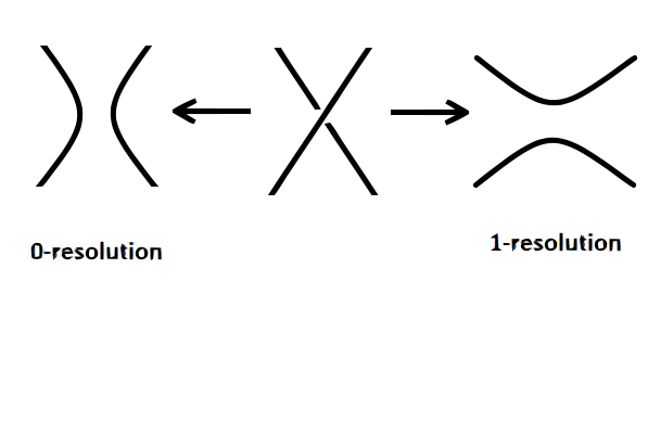
We denote $D(*0)$ and $D(*1)$ by the diagrams obtained by applying the 0-resolution and the 1-resolution at some fixed crossing of the link diagram $D$ as shown in the figure 4.

It is clear that $\mathcal{C}(D(*0))$ and $\mathcal{C}(D(*1))[-1]\{-1\}$ are subcomplexes of $\mathcal{C}(D)$ and form a short exact sequence

0\rightarrow\mathcal{C}(D(*1))[-1]\{-1\}\rightarrow\mathcal{C}(D)\rightarrow\mathcal{C}(D(*0))\rightarrow 0,

with degree preserving maps. Therefore, this induces a long exact sequence on homology:

(7)

\displaystyle\cdots\rightarrow\overline{\mathcal{H}}^{i-1,j}(D(*0))\stackrel{{\scriptstyle\delta}}{{\rightarrow}}\overline{\mathcal{H}}^{i-1,j-1}(D(*1))\rightarrow\overline{\mathcal{H}}^{i,j}(D)\rightarrow\overline{\mathcal{H}}^{i,j}(D(*0))\stackrel{{\scriptstyle\delta}}{{\rightarrow}}\overline{\mathcal{H}}^{i,j-1}(D(*1))\rightarrow\cdots

2.5. Lee Invariant

The Lee invariant is a variant of the rational Khovanov homology obtained from the same underlying complex, but with different differential. We let $H^{i}_{Lee}(L)$ to denote the $i-$ th homology group of the complex $\mathcal{C}(D)$ using Lee’s differential. The results needed from Lee’s invariant in this paper is summarized by

Proposition 2.6 (Proposition 3.3, [7]).

Let $L$ be an oriented link with $k$ components $L_{1},L_{2},\ldots,L_{k}$ . Then

(1)

$\dim(H_{Lee}(L))=2^{k}$ .
(2)

For every orientation $\theta$ of L there is a generator of homology in degree

$2\times\sum_{l\in E,m\in\bar{E}}lk(L_{l},L_{m})$

where $E\subset\{1,2,\ldots,k\}$ indexes the set of components of $L$ whose original orientation needs to be reversed to get the orientation $\theta$ and $\bar{E}=\{1,\ldots,k\}\setminus E$ . The linking numbers $lk(L_{l},L_{m})$ are the linking number (for the original orientation) between component $L_{l}$ and $L_{m}$ .
(3)

There is a spectral sequence converging to $H_{Lee}(L)$ with $E_{1}^{s,t}=\mathcal{H}^{s+t,4s}(L)$ .

2.6. Rasmussen $s$ -invariant

In [8] Rasmussen defines the $s$ -invariant as the average of the $j$ -gradings of the two copies of $\mathbb{Q}$ in the $H^{i}_{Lee}(K)$ which is the $E_{\infty}$ page of the above spectral sequence for the knot $K$ . He shows that the two $j$ -gradings differ by 2. Moreover, he shows that this invariant satisfies the following inequality:

(8)

\left|s(K)\right|\leq 2g^{*}(K),

where $g^{*}(K)$ is the slice genus of the knot $K$ .

3. The crossing number of Kanenobu knots

In this section, we establish the first goal of this paper that is evaluating the crossing number of Kanenobu knots $K(p,q)$ with $pq>0$ or $|pq|\leq\max\{|p|,|q|\}$ . In the case when $pq<0$ and $|pq|>\max\{|p|,|q|\}$ , we conjecture that the crossing number is $|p|+|q|+8$ . But first, we state and prove some results needed for the proof of the main theorem.

Proposition 3.1.

Let $\Br(V(p,q))$ denote the breadth of the Jones polynomial of Kanenobu knot $K(p,q)$ . Then,

\Br(V(p,q))=\begin{cases}{|p|+|q|+4},&\text{if $|p+q|>4$},\\ {8},&\text{if $|p+q|\leq 4$}.\end{cases}

Proof.

The Jones polynomial of the Kanenobu knot $V(p,q)$ is:

	$\displaystyle V(p,q)=$	$\displaystyle(-t)^{p+q}(V(0,0)-1)+1$
	$\displaystyle=$	$\displaystyle(-t)^{p+q}(t^{-4}-2t^{-3}+3t^{-2}-4t^{-1}+4-4t+3t^{2}-2t^{3}+t^{4})+1$
	$\displaystyle=$	$\displaystyle(-1)^{p+q}(t^{p+q-4}-2t^{p+q-3}+3t^{p+q-2}-4t^{p+q-1}+4t^{p+q}-4t^{p+q+1}+$
		$\displaystyle 3t^{p+q+2}-2t^{p+q+3}+t^{p+q+4})+1.$

We have three cases to consider

(1)

If $p+q<-4$ , then the highest and lowest exponents of $t$ in $V(p,q)$ are 0 and $p+q-4$ , respectively. So $\Br(V(p,q))=-p-q+4$ .
(2)

If $|p+q|\leq 4$ , then the highest and lowest exponents of $t$ in $V(p,q)$ are $p+q+4$ and $p+q-4$ , respectively. So $\Br(V(p,q))=8$ .
(3)

If $p+q>4$ , then the highest and lowest exponents of $t$ in $V(p,q)$ are $p+q+4$ and 0, respectively. So $\Br(V(p,q))=p+q+4$ .

∎

The $Q$ polynomial of any Kanenobu knot is given by the following proposition:

Proposition 3.2 (Proposition 4.5, [4]).

Let $Q(a,b)$ be the $Q$ polynomial of the Kanenobu knot $K(a,b)$ , then we have

\displaystyle Q(a,b)=-\sigma_{a}\sigma_{b}(Q(8_{9})-1)+x^{-1}(\sigma_{a+1}\sigma_{b+1}+\sigma_{a-1}\sigma_{b-1})(Q(8_{8})-1)+1,

where $Q(8_{8})=1+4x+6x^{2}-10x^{3}-14x^{4}+4x^{5}+8x^{6}+2x^{7}$ and $Q(8_{9})=-7+4x+16x^{2}-10x^{3}-16x^{4}+4x^{5}+8x^{6}+2x^{7}$ .

In the above proposition, $\sigma_{n}$ is defined as follows:

\sigma_{n}=\begin{cases}\frac{\alpha^{n}-\beta^{n}}{\alpha-\beta},&\text{if}\ n>0,\\ 0,&\text{if}\ n=0,\\ -\frac{\alpha^{-n}-\beta^{-n}}{\alpha-\beta},&\text{if}\ n<0,\end{cases}

where $\alpha+\beta=x$ and $\alpha\beta=1$ .

The degree of the $Q$ polynomial of any Kanenobu knot is given in the following proposition:

Proposition 3.3.

For the Kanenobu knot $K(p,q)$ , we have

\deg Q(p,q)=\begin{cases}|p|+|q|+6,&\text{if}\ pq\ \geq 0,\\ |p|+|q|+5,&\text{otherwise},\end{cases}

Proof.

We claim that $\sigma_{n}=\frac{n}{|n|}S_{|n|-1}(x)$ , where $S_{k}(x)$ is $k-th$ Chebyshev polynomial of the first kind which is defined inductively by $S_{-1}(x)=0,S_{0}(x)=1$ and $S_{k}(x)=xS_{k-1}(x)-S_{k-2}(x)$ . It is clear that this claim is true for $n=0,1$ . Now we prove this claim by showing that $(\alpha+\beta)\sigma_{k}=\sigma_{k+1}+\sigma_{k-1}$ for $k\geq 1$ . We prove the last statement as follows:

	$\displaystyle(\alpha+\beta)\sigma_{k}=$	$\displaystyle(\alpha+\beta)(\alpha^{k-1}+\alpha^{k-2}\beta+\ldots+\alpha\beta^{k-2}+\beta^{k-1})$
	$\displaystyle=$	$\displaystyle\alpha(\alpha^{k-1}+\alpha^{k-2}\beta+\ldots+\alpha\beta^{k-2}+\beta^{k-1})+$
		$\displaystyle\beta(\alpha^{k-1}+\alpha^{k-2}\beta+\ldots+\alpha\beta^{k-2}+\beta^{k-1})$
	$\displaystyle=$	$\displaystyle(\alpha^{k}+\alpha^{k-1}\beta+\ldots+\alpha^{2}\beta^{k-2}+\alpha\beta^{k-1})+$
		$\displaystyle(\alpha^{k-1}\beta+\alpha^{k-2}\beta^{2}+\ldots+\alpha\beta^{k-1}+\beta^{k})$
	$\displaystyle=$	$\displaystyle(\alpha^{k}+\alpha^{k-1}\beta+\ldots+\alpha^{2}\beta^{k-2}+\alpha\beta^{k-1}+\beta^{k})+$
		$\displaystyle(\alpha^{k-1}\beta+\alpha^{k-2}\beta^{2}+\ldots+\alpha\beta^{k-1})$
	$\displaystyle=$	$\displaystyle\sigma_{k+1}+(\alpha^{k-2}+\alpha^{k-3}\beta+\ldots+\beta^{k-2})=\sigma_{k+1}+\sigma_{k-1},$

where we used the fact that $\alpha\beta=1$ in the equation before the last one. Now the claim follows since we have that $\sigma_{n}=-\sigma_{-n}$ for $n<0$ .

Finally, the result follows since we have $\deg Q(p,q)=\deg(\sigma_{|p|+1}\sigma_{|q|+1})+\deg Q(8_{8})-1=|p|+|q|+7-1=|p|+|q|+6$ for $pq\geq 0$ and $\deg Q(p,q)=\deg(\sigma_{|p+1|}\sigma_{|q+1|})+\deg Q(8_{8})-1=|p|+|q|+7-1-1=|p|+|q|+5$ for $pq<0$ .

In the above argument we used the that $\deg 0=-1$ . ∎

The main tool in proving our main theorem in this section is the following:

Theorem 3.4 (Main Theorem, [6]).

Let $D$ be a diagram of a link $L$ . Then,

(9)

\displaystyle\deg Q\leq c(D)-b(D)

where $c(D)$ is the crossing number of the diagram $D$ of $L$ , $b(D)$ is the maximal bridge length of $D$ , i.e., the maximal number of consecutive over-pass or under-passes crossings and $\deg Q$ is the degree of the $Q$ polynomial of the link $L$ . Moreover, if $D$ is alternating (i.e. $b(D)$ = 1) and prime, then equality holds.

Theorem 3.5.

The crossing number of the Kanenobu knot $K(p,q)$ is given as follows:

c(K(p,q))=\begin{cases}|p|+|q|+6,&\text{if}\ pq<0\ \text{and}\ |p|+|q|=2,\\ |p|+|q|+7,&\text{if}\ \left(pq<0\ \text{and}\ (|p|=1\ \text{or}\ |q|=1\ \text{but not both})\right)\\ &\text{or}\ \left(pq=0\ \text{and}\ |p|+|q|=1\right),\\ |p|+|q|+8,&\text{if}\ pq>0\ \text{or}\ \left(pq=0\ \text{and}\ |p|+|q|\neq 1\right).\end{cases}

Proof.

We give the proof case by case

(1)

If $pq<0$ and $|p|+|q|=2$ , then we have $(p,q)=(1,-1)$ or $(p,q)=(-1,1)$ . We have used Reidemeister moves to construct a reduced alternating diagram of $K(1,-1)$ of 8 crossings as shown in figure 6. So by the third part of Theorem 2.3 we obtain $c(K(1,-1))=8=|1|+|-1|+6$ . Now $c(K(-1,1))=c(K(1,-1))=8$ as a result of Proposition 1.2.
(2)
We have two subcases that will be treated separately
1. (a)
  
  If $pq<0$ and $(|p|=1$ or $|q|=1$ but not both), then we have $(p,q)=(m,-1)$ or $(p,q)=(-1,m)$ or $(p,q)=(-m,1)$ or $(p,q)=(1,-m)$ for a positive integer $m$ . We have used Reidemeister moves to construct a diagram of $K(m,-1)$ with $m+8$ crossings as shown in figure 7. Now by Theorem 3.4 and Proposition 3.3, we have
  
  $\deg Q(m,-1)=m+1+5=m+6\leq c(D)-b(D),$
  
  which implies that $c(D)\geq m+6+b(D)$ for any knot diagram $D$ of $K(m,-1)$ . We have $b(D)\geq 2$ for any knot diagram $D$ of the knot $K(p,-1)$ since this knot is not alternating. i, e $b(D)\geq 2$ . This follows since if it is alternating, then by Theorem 3.4, we would have $c(K(m,-1))=\deg Q(m,-1)+1=m+7=\Br(V(m,-1))=8$ or $c(K(m,-1))=\deg Q(m,-1)+1=m+7=\Br(V(m,-1))=m+1+4$ which is impossible in both cases. Now the result follows since we have already constructed a diagram of $m+8$ crossings with $b(D)=2$ . Now $c(K(m,-1))=c(K(-m,1))=c(K(1,m))=c(K(1,-m))=m+1+7=m+8$ as a result of Proposition 1.2.
2. (b)
  
  If $pq=0\ \text{and}\ |p|+|q|=1$ , then $(p,q)=(1,0)$ or $(p,q)=(-1,0)$ or $(p,q)=(0,1)$ or $(p,q)=(0,-1)$ . It is enough to consider one case of these four cases as a result of Proposition 1.2. We have used Reidemeister moves to construct a reduced alternating diagram of $K(1,0)$ of 8 crossings as shown in figure 5. So by the third part of Theorem 2.3 we obtain $c(K(1,0))=8=|1|+|0|+7$ . Now $c(K(0,1))=c(K(-1,0))=c(K(0,-1))=c(K(1,0))=8=|1|+|0|+7$ as a result of Proposition 1.2.
(3)
We have two also two subcases that will be treated separately
1. (a)
  
  If $pq>0$ , then both of $p$ and $q$ are positive or negative integers. Now by Theorem 3.4 and Proposition 3.3, we have
  
  $\deg Q(p,q)=|p|+|q|+6\leq c(D)-b(D),$
  
  which implies that $c(D)\geq|p|+|q|+6+b(D)$ for any knot diagram $D$ of $K(p,q)$ . We have $b(D)\geq 2$ for any knot diagram $D$ of the knot $K(p,q)$ since this knot is not alternating. This follows since if it is alternating, then by Theorem 3.4, we would have $c(K(p,q))=\deg Q(p,q)+1=|p|+|q|+7=\Br(V(p,q))=8$ or $c(K(p,q))=\deg Q(p,q)+1=|p|+|q|+7=\Br(V(p,q))=|p|+|q|+4$ which is impossible in both cases. Now the result follows since we have already a diagram of $|p|+|q|+8$ crossings with $b(D)=2$ .
2. (b)
  
  If $pq=0$ and $|p|+|q|\neq 1$ , then we have $(p,q)=(m,0)$ or $(p,q)=(0,m)$ for $m\neq\pm 1$ . Now by Theorem 3.4 and Proposition 3.3, we have
  
  $\deg Q(m,0)=|m|+6\leq c(D)-b(D),$
  
  which implies that $c(D)\geq|m|+6+b(D)$ for any knot diagram $D$ of $K(m,0)$ . We have $b(D)\geq 2$ for any knot diagram $D$ of the knot $K(m,0)$ since this knot is not alternating. This follows since if it is alternating, then by Theorem 3.4, we would have $c(K(m,0))=\deg Q(m,0)+1=|m|+7=\Br(V(m,0))=8$ or $c(K(m,0))=\deg Q(m,0)+1=|m|+7=\Br(V(m,0))=|m|+4$ which is impossible in both cases. Now the result follows since we have already a diagram of $|m|+8$ crossings with $b(D)=2$ . Now $c(K(m,0))=c(K(0,m))=|m|+8$ as a result of Proposition 1.2.

∎

Corollary 3.6.

The Kanenobu knots $K(p,q)$ are not alternating except for $K(0,0),\\ K(1,0),K(0,1),K(-1,0),K(0,-1),K(1,-1)$ and $K(-1,1)$ .

Figure 5. Using Reidemeister moves to construct a reduced alternating diagram of

K(1,0)

Figure 6. Using Reidemeister moves to construct a reduced alternating diagram of

K(1,-1)

Figure 7. Using Reidemeister moves to construct a reduced diagram of

K(p,-1)

Proposition 3.7.

For the case when $pq<0$ with $|p|\neq 1$ and $|q|\neq 1$ , we have $|p|+|q|+7\leq c(K(p,q))\leq|p|+|q|+8$ .

Proof.

We have $\deg Q(p,q)=|p|+|q|+5$ with a knot diagram of $|p|+|q|+8$ crossings. We also know that the knot $K(p,q)$ in this case is not alternating. This follows since if it is alternating, then by Theorem 3.4, we would have $c(K(p,q))=\deg Q(p,q)+1=|p|+|q|+6=\Br(V(p,q))=8$ or $c(K(p,q))=\deg Q(p,q)+1=|p|+|q|+6=\Br(V(p,q))=|p|+|q|+4$ which is impossible in both cases.

∎

We suggest the following conjecture that computes the crossing number of the Kanenobu knot $K(p,q)$ in the above case.

Conjecture 3.8.

For the case when $pq<0$ with $|p|\neq 1$ and $|q|\neq 1$ , we have $c(K(p,q))\leq|p|+|q|+8$ .

4. Khovanov homology of Kanenobu knots

Lemma 4.1.

The Khovanov bigraded homology groups of the figure eight knot $\mathcal{H}^{i,j}(K)$ are given as follows:

\dim\mathcal{H}^{i,j}(K)=\begin{cases}1,&\text{if}\ {(i,j)=(-2,-5),(-1,-1),(0,-1),(0,1),(1,1),(2,5)},\\ 0,&\text{otherwise}.\\ \end{cases}

Lemma 4.2.

The Kanenobu knot $K(p,0)$ is a slice knot. Therefore, we obtain $s(K(p,0))=0$ .

Proof.

We know that the knot $K(p,0)$ is a ribbon knot by Theorem 6, so it is a slice knot. The second part follows by inequality 8. ∎

Lemma 4.3.

We have

	$\displaystyle\dim\overline{\mathcal{H}}^{x(D),2x(D)-y(D)-1}(D)$	$\displaystyle=\dim\overline{\mathcal{H}}^{x(D)+1,2x(D)-y(D)+3}(D)+1,$
	$\displaystyle\dim\overline{\mathcal{H}}^{x(D),2x(D)-y(D)+1}(D)$	$\displaystyle=\dim\overline{\mathcal{H}}^{x(D)-1,2x(D)-y(D)-3}(D)+1,$
	$\displaystyle\dim\mathcal{H}^{i,j}(K)$	$\displaystyle=\dim\mathcal{H}^{i+1,j+4}(K)+1.$

for any diagram $D$ of a homologically thin knot $K$ with $s(K)=0$ and $j-2i=\sigma(K)-1$ .

The following lemma will be used later in this paper.

Lemma 4.4.

$\sigma(K(p,0))=0$ for any integer $p$ .

Proposition 4.5.

The Khovanov bigraded homology groups of the disjoint union of two figure eight knots $K\sqcup K$ are given by the following:

\dim\mathcal{H}^{i,j}(K\sqcup K)=\begin{cases}1,&\text{if}\ {(i,j)=(-4,-10),(-2,-2),(0,-2),(0,2),(2,2),(4,10)},\\ 2,&\text{if}\ {(i,j)=(-3,-6),(-2,-6),(-2,-4),(-1,-4),(-1,-2)},\\ &{\qquad\qquad\ (-1,0),(1,0),(1,2),(1,4),(2,4),(2,6),(3,6)},\\ 6,&\text{if}\ {(i,j)=(0,0)},\\ 0,&\text{otherwise}.\\ \end{cases}

Proof.

We use $\mathcal{H}^{i,j}(K\sqcup K)={\bigoplus}_{l,m\in\mathbb{Z}}(\mathcal{H}^{l,m}(K)\otimes\mathcal{H}^{i-l,j-m}(K))$ given in [Corollary 12, [5]]. ∎

Proposition 4.6.

The Khovanov bigraded homology groups of the Kanenobu knot $K(0,0)$ are given by the following:

\dim\mathcal{H}^{i,j}(K(0,0))=\begin{cases}1,&\text{if}\ {(i,j)=(-4,-9),(-3,-7),(-3,-5),(-2,-3),(2,3)},\\ &\qquad\qquad\ (3,5),(3,7),(4,9),\\ 2,&\text{if}\ {(i,j)=(-2,-5),(-1,-3),(-1,-1),(1,1),(1,3),(2,5)},\\ 3,&\text{if}\ {(i,j)=(0,-1),(0,1)},\\ 0,&\text{otherwise}.\\ \end{cases}

Proof.

It is well-know that the Kanenobu knot $K(0,0)$ is the connected sum of two figure eight knots $K\#K$ . We use the following long exact sequence given in [Proposition 34, [5]]:

\ldots\rightarrow\mathcal{H}^{i-1,j-1}(K\sqcup K)\rightarrow\mathcal{H}^{i-1,j-2}(K\#K)\rightarrow\mathcal{H}^{i,j}(K\#K)\rightarrow\mathcal{H}^{i,j-1}(K\sqcup K)\rightarrow\ldots

We consider cases by case

(1)

If $j=9$ then we have two subcases

(a)

If $i=4$

	$\displaystyle\ldots\rightarrow\mathcal{H}^{4,11}(K\#K)\rightarrow\mathcal{H}^{4,10}(K\sqcup K)\rightarrow$	$\displaystyle\mathcal{H}^{4,9}(K\#K)\rightarrow\mathcal{H}^{5,11}(K\#K)\rightarrow\ldots$
	$\displaystyle 0\rightarrow\mathbb{Q}\rightarrow$	$\displaystyle\mathcal{H}^{4,9}(K\#K)\rightarrow 0,$

so we get $\dim\mathcal{H}^{4,9}(K\#K)=1$ .

(b)

If $i=5$

	$\displaystyle\ldots\rightarrow\mathcal{H}^{5,11}(K\#K)\rightarrow\mathcal{H}^{5,10}(K\sqcup K)\rightarrow$	$\displaystyle\mathcal{H}^{5,9}(K\#K)\rightarrow\mathcal{H}^{6,11}(K\#K)\rightarrow\ldots$
	$\displaystyle 0\rightarrow 0\rightarrow$	$\displaystyle\mathcal{H}^{5,9}(K\#K)\rightarrow 0,$

so we get $\dim\mathcal{H}^{5,9}(K\#K)=0$ .

(2)

If $j=7$ then we have two subcases

(a)

If $i=3$

	$\displaystyle\ldots\rightarrow\mathcal{H}^{3,8}(K\sqcup K)\rightarrow\mathcal{H}^{3,7}(K\#K)\rightarrow$	$\displaystyle\mathcal{H}^{4,9}(K\#K)\rightarrow\mathcal{H}^{4,8}(K\sqcup K)\rightarrow\ldots$
	$\displaystyle 0\rightarrow\mathcal{H}^{3,7}(K\#K)\rightarrow$	$\displaystyle\mathcal{H}^{4,9}(K\#K)\rightarrow 0,$

so we get $\dim\mathcal{H}^{3,7}(K\#K)=\dim\mathcal{H}^{4,9}(K\#K)=1$ .

(b)

If $i=4$

	$\displaystyle\ldots\rightarrow\mathcal{H}^{4,8}(K\sqcup K)\rightarrow\mathcal{H}^{4,7}(K\#K)\rightarrow$	$\displaystyle\mathcal{H}^{5,9}(K\#K)\rightarrow\mathcal{H}^{5,8}(K\#K)\rightarrow\ldots$
	$\displaystyle 0\rightarrow\mathcal{H}^{4,7}(K\#K)\rightarrow$	$\displaystyle\mathcal{H}^{5,9}(K\#K)\rightarrow 0,$

so we get $\dim\mathcal{H}^{4,7}(K\#K)=\dim\mathcal{H}^{5,9}(K\#K)=0$ .

(3)

If $j=5$ , then we have

	$\displaystyle\ldots\rightarrow\mathcal{H}^{2,7}(K\#K)\rightarrow\mathcal{H}^{2,6}(K\sqcup K)\rightarrow$	$\displaystyle\mathcal{H}^{2,5}(K\#K)\rightarrow\mathcal{H}^{3,7}(K\#K)$
	$\displaystyle\rightarrow\mathcal{H}^{3,6}(K\sqcup K)$	$\displaystyle\rightarrow\mathcal{H}^{3,5}(K\#K)\rightarrow\mathcal{H}^{4,7}(K\#K)\rightarrow\ldots$
	$\displaystyle 0\rightarrow\mathbb{Q}\oplus\mathbb{Q}\rightarrow\mathcal{H}^{2,5}(K\#K)\rightarrow$	$\displaystyle\mathbb{Q}\rightarrow\mathbb{Q}\oplus\mathbb{Q}\rightarrow\mathcal{H}^{3,5}(K\#K)\rightarrow 0,$

Now we have $\dim\mathcal{H}^{3,5}(K\#K)=\dim\mathcal{H}^{4,9}(K\#K)=1$ as a result of the third statement of Lemma 4.3. Therefore, we obtain $\dim\mathcal{H}^{2,5}(K\#K)=2$ since the Euler characteristic of an exact sequence must vanish.

(4)

If $j=3$ , then we have

	$\displaystyle\ldots\rightarrow\mathcal{H}^{1,5}(K\#K)\rightarrow\mathcal{H}^{1,4}(K\sqcup K)\rightarrow$	$\displaystyle\mathcal{H}^{1,3}(K\#K)\rightarrow\mathcal{H}^{2,5}(K\#K)$
	$\displaystyle\rightarrow\mathcal{H}^{2,4}(K\sqcup K)\rightarrow\mathcal{H}^{2,3}(K\#K)\rightarrow$	$\displaystyle\mathcal{H}^{3,5}(K\#K)\rightarrow\mathcal{H}^{3,4}(K\sqcup K)\rightarrow\ldots$
	$\displaystyle 0\rightarrow\mathbb{Q}\oplus\mathbb{Q}\rightarrow\mathcal{H}^{1,3}(K\#K)\rightarrow\mathbb{Q}\oplus\mathbb{Q}\rightarrow$	$\displaystyle\mathbb{Q}\oplus\mathbb{Q}\rightarrow\mathcal{H}^{2,3}(K\#K)\rightarrow\mathbb{Q}\rightarrow 0,$

Now we have $\dim\mathcal{H}^{2,3}(K\#K)=\dim\mathcal{H}^{3,7}(K\#K)=1$ as a result of the third statement of Lemma 4.3. Therefore, we obtain $\dim\mathcal{H}^{1,3}(K\#K)=2$ since the Euler characteristic of an exact sequence must vanish.

(5)

If $j=1$ , then we have

	$\displaystyle\ldots\rightarrow\mathcal{H}^{0,3}(K\#K)\rightarrow\mathcal{H}^{0,2}(K\sqcup K)\rightarrow$	$\displaystyle\mathcal{H}^{0,1}(K\#K)\rightarrow\mathcal{H}^{1,3}(K\#K)$
	$\displaystyle\rightarrow\mathcal{H}^{1,2}(K\sqcup K)\rightarrow\mathcal{H}^{1,1}(K\#K)\rightarrow$	$\displaystyle\mathcal{H}^{2,3}(K\#K)\rightarrow\mathcal{H}^{2,2}(K\sqcup K)\rightarrow\mathcal{H}^{2,1}(K\#K)\rightarrow\ldots$
	$\displaystyle 0\rightarrow\mathbb{Q}\rightarrow\mathcal{H}^{0,1}(K\#K)\rightarrow\mathbb{Q}\oplus\mathbb{Q}\rightarrow$	$\displaystyle\mathbb{Q}\oplus\mathbb{Q}\rightarrow\mathcal{H}^{1,1}(K\#K)\rightarrow\mathcal{H}^{2,3}(K\#K)\rightarrow\mathbb{Q}\rightarrow 0,$

Now we have $\dim\mathcal{H}^{1,1}(K\#K)=\dim\mathcal{H}^{2,5}(K\#K)=2$ as a result of the third statement of Lemma 4.3. Also, we have $\dim\mathcal{H}^{0,1}(K\#K)\dim\mathcal{H}^{-1,-3}(K\#K)+1=\dim\mathcal{H}^{1,3}(K\#K)+1=3$ . The last isomorphism follows as a result of Theorem 1.2 and [Corollary 11,[5]]. Therefore, we obtain $\dim\mathcal{H}^{2,3}(K\#K)=1$ since the Euler characteristic of an exact sequence must vanish.

Finally the result follows by [Corollary 11,[5]] since $K\#K$ is equivalent to its mirror image. ∎

Theorem 4.7.

The Kanenobu knot $K(p,0)$ for a negative integer $p$ is homologically thin over $\mathbb{Q}$ and its Khovanov bigraded homology groups are given as follows:

\dim\mathcal{H}^{i,j}(K(p,0))=\begin{cases}\dim\mathcal{H}^{-p,-2p-1}(K(0,0))+1,&\text{if}\ {(i,j)=(0,1)},\\ \dim\mathcal{H}^{-p,-2p+1}(K(0,0))+1,&\text{if}\ {(i,j)=(0,-1),}\\ \dim\mathcal{H}^{-p-1,-2p-3}(K(0,0)),&\text{if}\ {(i,j)=(-1,-3)\ \text{and}\ p\neq-1},\\ \dim\mathcal{H}^{-p-1,-2p-1}(K(0,0)),&\text{if}\ {(i,j)=(-1,-1)\ \text{and}\ p\neq-1},\\ \dim\mathcal{H}^{0,1}(K(0,0))-1,&\text{if}\ {(i,j)=(p,2p+1)},\\ \dim\mathcal{H}^{0,-1}(K(0,0))-1,&\text{if}\ {(i,j)=(p,2p-1)},\\ \dim\mathcal{H}^{i+p,j+2p}(K(0,0)),&\text{otherwise}.\\ \end{cases}

Proof.

We show the claim by induction on $|p|$ . We resolve any crossing of the $p$ -crossings to obtain $D(*0)$ and $D(*1)$ . It is clear that $D(*0)$ is a diagram of the Kanenobu knot $K(p+1,0)$ and $D(*1)$ is a diagram of the unlink of two components as seen in figure 8.

From the induction hypothesis, $K(p+1,0)$ is homologically thin. Therefore, $\mathcal{H}(K(p+1,0))$ is supported on the two lines $j-2i=\sigma(K(p+1,0))\pm 1=\pm 1$ . As $x(K(p+1,0))=x(D(*1))=3-p$ and $y(K(p+1,0))=y(D(*1))=4$ , then $\overline{\mathcal{H}}(K(p+1,0))$ is supported on the two lines $j-2i=-4\pm 1$ . Also, we have

\overline{\mathcal{H}}^{i,j}(D(*1))=\begin{cases}\mathbb{Q},&\text{if $(i,j)=(3-p,4-2p)$, or $(3-p,-2p)$},\\ \mathbb{Q}\oplus\mathbb{Q},&\text{if $(i,j)=(3-p,2-2p)$},\\ 0,&\text{otherwise}.\end{cases}

Now we obtain $\dim\overline{\mathcal{H}}^{i,j}(K(p,0))=\dim\overline{\mathcal{H}}^{i,j}(K(p+1,0))$ directly from the long exact sequence on homology except on the following three cases:

(1)

0\rightarrow\mathbb{Q}\rightarrow\overline{\mathcal{H}}^{4-p,5-2p}(K(p,0))\rightarrow\overline{\mathcal{H}}^{4-p,5-2p}(K(p+1,0))\rightarrow 0.

Therefore, we obtain $\dim\overline{\mathcal{H}}^{4-p,5-2p}(K(p,0))=\dim\overline{\mathcal{H}}^{4-p,5-2p}(K(p+1,0))+1$ .

(2)

0\rightarrow\overline{\mathcal{H}}^{3-p,1-2p}(K(p,0))\rightarrow\overline{\mathcal{H}}^{3-p,1-2p}(K(p+1,0))\stackrel{{\scriptstyle\delta}}{{\rightarrow}}\mathbb{Q}\rightarrow\overline{\mathcal{H}}^{4-p,1-2p}(K(p,1))\rightarrow 0.

We have two subcases and only the second one holds:

(a)

$\dim\overline{\mathcal{H}}^{3-p,1-2p}(K(p,0))=\dim\overline{\mathcal{H}}^{3-p,1-2p}(K(p+1,0))$ and

$\dim\overline{\mathcal{H}}^{4-p,1-2p}(K(p,0))=1$ . By induction, $K(p+1,0)$ is homologically thin. So by Lemma 4.3, we obtain $\dim\overline{\mathcal{H}}^{3-p,1-2p}(K(p+1,0))=\dim\overline{\mathcal{H}}^{4-p,5-2p}(K(p+1,0))+1$ . Hence we conclude $\dim\overline{\mathcal{H}}^{3-p,1-2p}(K(p,0))=\dim\overline{\mathcal{H}}^{4-p,5-2p}(K(p,0))$ . Now in the spectral sequence:

0\rightarrow\overline{\mathcal{H}}^{3-p,1-2p}(K(p,0))\stackrel{{\scriptstyle d_{1}}}{{\rightarrow}}\overline{\mathcal{H}}^{4-p,5-2p}(K(p,0))\rightarrow 0.

The map $d_{1}$ has to be injective and not surjective since in the $E_{\infty}$ -page one copy of $\mathbb{Q}$ survives at the $j$ -grading 1 and not at the $j$ -grading -3. This is impossible as the domain and the codomain have the same dimension.

(b)

$\dim\overline{\mathcal{H}}^{3-p,1-2p}(K(p,0))=\dim\overline{\mathcal{H}}^{3-p,1-2p}(K(p+1,0))-1,$ and

$\dim\overline{\mathcal{H}}^{4-p,1-2p}(D)=0$ .

(3)

		$\displaystyle 0\rightarrow\overline{\mathcal{H}}^{3-p,3-2p}(K(p,0))\rightarrow\overline{\mathcal{H}}^{3-p,3-2p}(K(p+1,0))\stackrel{{\scriptstyle\delta}}{{\rightarrow}}\mathbb{Q}\oplus\mathbb{Q}$
		$\displaystyle\rightarrow\overline{\mathcal{H}}^{4-p,3-2p}(K(p,0))\rightarrow\overline{\mathcal{H}}^{4-p,3-2p}(K(p+1,0))\rightarrow 0.$

We conclude that the Kanenobu knot $K(p,0)$ is homologically thin as the its bigraded homology is supported on $j-2i=-4\pm 1$ . Therefore as a result of the third statement of Lemma 4.3, we obtain

	$\displaystyle\dim\overline{\mathcal{H}}^{3-p,3-2p}(K(p,0))+1$	$\displaystyle=\dim\overline{\mathcal{H}}^{2-p,-1-2p}(K(p,0))+1$
		$\displaystyle=\dim\overline{\mathcal{H}}^{2-p,-1-2p}(K(p+1,0))+1$
		$\displaystyle=\dim\overline{\mathcal{H}}^{3-p,3-2p}(K(p+1,0)).$

Also since the Euler characteristic of an exact sequence must vanish, we obtain

\displaystyle\dim\overline{\mathcal{H}}^{4-p,3-2p}(K(p,0))=\dim\overline{\mathcal{H}}^{4-p,3-2p}(K(p+1,0))+1.

Finally, the recursion holds from the fact that $x(K(p,0))=4-p$ and $y(K(p,0))=4$ and equation 5. ∎

As a result of Theorem 1.2 and [Corollary 11,[5]], we obtain

Corollary 4.8.

The Kanenobu knot $K(p,0)$ for a positive integer $p$ is homologically thin over $\mathbb{Q}$ and its Khovanov bigraded homology groups are given by $\mathcal{H}^{i,j}(K(p,0))=\mathcal{H}^{-i,-j}(K(-p,0))$ .

We show that $\mathcal{H}^{i,j}(K(p,q))$ depends only on the sum of $p$ and $q$ and this generalizes [Theorem 7, [2]]. So we can compute the rational Khovanov bigraded homology groups of any Kanenobu knot by combining Theorem 4.7 and Corollary 4.8.

Proposition 4.9.

For any two integers $p$ and $q$ , we have

\mathcal{H}^{i,j}(K(p,q))\equiv\mathcal{H}^{i,j}(K(p+q,0)).

Proof.

We can assume that $p<0$ and $|p|>q$ using the second part of Proposition 1.2. We have $x(K(p,q))=x(K(p+q,0)),y(K(p,q))=y(K(p+q,0)),x(K(p+1,q))=x(K(p+q+1,0)),y(K(p+1,q))=y(K(p+q+1,0)),$ and $x(U_{1})=x(U_{2}),y(U_{1})=y(U_{2}),$ where $U_{1}$ and $U_{2}$ are diagrams of the unlink of two components obtained by resolving one of the $p$ -th and $p+q$ -th crossings in the diagrams of $K(p,q)$ and $K(p+q,0)$ respectively. Therefore, it is enough to show that $\overline{\mathcal{H}}^{i,j}(K(p,q))\equiv\overline{\mathcal{H}}^{i,j}(K(p+q,0))$ .

The long exact sequences for $K(p,q)$ and $K(p+q,0)$ as in equation 7 are isomorphic as seen in the following commutative diagram using the five lemma if we use induction on $|p+q|$ . ∎

$\begin{CD}\overline{\mathcal{H}}^{i-1,j}(K(p+1,q))@>{}>{}>\overline{\mathcal{H}}^{i-1,j-1}(U_{1})@>{}>{}>\overline{\mathcal{H}}^{i,j}(K(p,q))@>{}>{}>\overline{\mathcal{H}}^{i,j}(K(p+1,q))@>{}>{}>\overline{\mathcal{H}}^{i,j-1}(U_{1})\\ \Big\|\Big\|@V{}V{}V\Big\|\Big\|\\ \overline{\mathcal{H}}^{i-1,j}(K(p+q+1,0))@>{}>{}>\overline{\mathcal{H}}^{i-1,j-1}(U_{2})@>{}>{}>\overline{\mathcal{H}}^{i,j}(K(p+q,0))@>{}>{}>\overline{\mathcal{H}}^{i,j}(K(p+q+1,0))@>{}>{}>\overline{\mathcal{H}}^{i,j-1}(U_{2})\end{CD}$

References

[1] R.D. Brandt, W.B.R. Lickorish, and K.C. Millett: A polynomial invariant for unoriented knots and links, Invent. Math. 84 (1986), 563–573.
[2] J. Greene, and L. Watson: Turaev Torsion, definite 4-manifolds, and quasi-alternating knots, Bull. London Math. Soc. 45 (5) (2013), 962-972.
[3] T. Kanenobu: Infinitely Many Knots with the Same Polynomial Invariant, Proc. Amer. Math. Soc. 97 (1) (1986), 158–162.
[4] T. Kanenobu: Examples on Polynomial Invariants of Knots and Links, Math. Ann. 275 (1986), 555–572.
[5] M. Khovanov: A categorification of the Jones polynomial, Duke Math. J. 101 (3) (2000), 359–426.
[6] M. Kidwell: On the Degree of the Brandt-Lickorish-Millett-Ho Polynomial of a Link, Proc. Amer. Math. Soc. 100 (4) (1987), 755–762.
[7] E. S. Lee: An endomorphism of the Khovanov invariant, Adv. Math. 197 (2) (2005), 554-586.
[8] J. Rasmussen: Khovanov homology and the slice genus, Invent. Math. 182 (2) (2010), 419-447.
[9] M. Thistlethwaite: A Spanning tree expansion of the Jones polynomial, Topology 26 (3) (1987), 297-309.

Further Study of Kanenobu Knots

Abstract.

Key words and phrases:

2000 Mathematics Subject Classification

1. Introduction

Theorem 1.1 (Main Theorem, [3]).

Proposition 1.2 ([3, 4]).

2. Background and Notations

2.1. The Jones Polynomial

Definition 2.1.

Proposition 2.2.

Theorem 2.3 (Theorem 1 & 2 & Corollary 1, [9]).

2.2. The Kauffman Polynomial

Definition 2.4.

Proposition 2.5 (Property 2, [1]).

2.3. Khovanov Invariant

2.4. Exact Sequence

2.5. Lee Invariant

Proposition 2.6 (Proposition 3.3, [7]).

2.6. Rasmussen ss-invariant

3. The crossing number of Kanenobu knots

Proposition 3.1.

Proof.

Proposition 3.2 (Proposition 4.5, [4]).

Proposition 3.3.

Proof.

Theorem 3.4 (Main Theorem, [6]).

Theorem 3.5.

Proof.

Corollary 3.6.

Proposition 3.7.

Proof.

Conjecture 3.8.

4. Khovanov homology of Kanenobu knots

Lemma 4.1.

Lemma 4.2.

Proof.

Lemma 4.3.

Lemma 4.4.

Proposition 4.5.

Proof.

Proposition 4.6.

Proof.

Theorem 4.7.

Proof.

Corollary 4.8.

Proposition 4.9.

Proof.

References

2.6. Rasmussen $s$ -invariant