Effective Spectral Function for Quasielastic Scattering on Nuclei
Abstract
Spectral functions that are used in neutrino event generators to model quasielastic (QE) scattering from nuclear targets include Fermi gas, Local Thomas Fermi gas (LTF), Bodek-Ritchie Fermi gas with high momentum tail, and the Benhar-Fantoni two dimensional spectral function. We find that the dependence of predictions of these spectral functions for the QE differential cross sections () are in disagreement with the prediction of the superscaling function which is extracted from fits to quasielastic electron scattering data on nuclear targets. It is known that spectral functions do not fully describe quasielastic scattering because they only model the initial state. Final state interactions distort the shape of the differential cross section at the peak and increase the cross section at the tails of the distribution. We show that the kinematic distributions predicted by the superscaling formalism can be well described with a modified effective spectral function (ESF). By construction, models using ESF in combination with the transverse enhancement contribution correctly predict electron QE scattering data.
pacs
13.15.+gNeutrino interactions and 25.30.PtNeutrino scattering and 25.30.Dh, 25.30.Fj electron scattering inelastic1 Introduction
Neutrino oscillation experiments make use of neutrino Monte Carlo (MC) event generators to model the cross sections and kinematic distributions of the leptonic and hadronic final state of neutrino interactions on nuclear targets. Therefore, reliable simulations of the effects of Fermi motion and other nuclear effects are important. In order to model neutrino cross sections we need to model the vector part, the axial-vector part, and axial-vector interference. Because of the conservation of the vector current (CVC), the same models should be able to reliably predict the QE electron scattering cross section on nuclear targets. Unfortunately, none of the models which are currently implemented in neutrino MC generators are able to do it. In this paper, we propose an approach which guarantees agreement with quasielaststic (QE) electron scattering data by construction.
1.1 QE Scattering from independent nucleons


The top panel of Fig. 1 is the general diagram for QE lepton (election, muon or neutrino) scattering from a nucleon which is bound in a nucleus of mass . In this paper, we focus on charged current neutrino scattering. The scattering is from an off-shell bound neutron of momentum . The on-shell recoil (spectator) nucleus has a momentum . This process is referred to as the 1p1h process (one proton one hole). The * is used to indicate that the spectator nucleus is not in the ground state because it has one hole. The four-momentum transfer to the nuclear target is defined as . Here is the energy transfer, and is the square of the four-momentum transfer. For free nucleons the energy transfer is equal to where is the mass of the nucleon. At a fixed value of , QE scattering on nucleons bound in a nucleus yields a distribution in which peaks at . In this communication, the term ”normalized quasielastic distribution” refers to the normalized differential cross section where is the integral of over all values of (for a given value of ).
The bottom panel of Fig. 1 shows the same QE lepton scattering process, but now also including a final state interaction with another nucleon in the scattering process. This final state interaction modifies the scattering amplitude and therefore can change the kinematics of the final state lepton. In this paper, we refer to it as ”final state interaction of the first kind” (FSI).
The final state nucleon can then undergo more interactions with other nucleons in the spectator nucleus. These interactions do not change the energy of the final state lepton. We refer to this kind of final state interaction as ”final state interaction of the second kind”. Final state interactions of the second kind reduce the energy of the final state nucleon.
1.2 Spectral functions
In general, neutrino event generators assume that the scattering occurs on independent nucleons which are bound in the nucleus. Generators such as GENIE[1], NEUGEN[2], NEUT[3], NUANCE[4] NuWro [5] and GiBUU[6] account for nucleon binding effects by modeling the momentum distributions and removal energy of nucleons in nuclear targets. Functions that describe the momentum distributions and removal energy of nucleons from nuclei are referred to as spectral functions.
Spectral functions can take the simple form of a momentum distribution and a fixed removal energy (e.g. Fermi gas model[7]), or the more complicated form of a two dimensional (2D) distribution in both momentum and removal energy (e.g. Benhar-Fantoni spectral function [8]).
Fig. 2 shows the nucleon momentum distributions in a nucleus for some of the spectral functions that are currently being used. The solid green line is the nucleon momentum distribution for the Fermi gas[7] model (labeled ”Global Fermi” gas) which is currently implemented in all neutrino event generators is given in equation 30 of Appendix B). The solid black line is the projected momentum distribution of the Benhar-Fantoni [8] 2D spectral function as implemented in NuWro. The solid red line is the nucleon momentum distribution of the Local-Thomas-Fermi gas (LTF) model[6] which is implemented in NURWO and GiBUU.
It is known that theoretical calculations using spectral functions do not fully describe the shape of the quasielastic peak for electron scattering on nuclear targets . This is because the calculations only model the initial state (shown on the top panel of Fig. 1), and do not account for final state interactions of the first kind (shown on the bottom panel of Fig. 1) . Because FSI changes the amplitude of the scattering, it modifies the shape of . FSI reduces the cross section at the peak and increases the cross section at the tails of the distribution.
In contrast to the spectral function formalism, predictions using the superscaling formalism[9, 10] fully describe the longitudinal response function of quasielastic electron scattering data on nuclear targets. This is expected since the calculations use a superscaling function which is directly extracted from the longitudinal component of measured electron scattering quasielastic differential cross sections.
However, although superscaling provides a very good description of the final state lepton in QE scattering, superscaling is not implemented as an option in neutrino MC event generators that are currently used neutrino experiments. There are specific technical issues that are associated with implementing any theoretical model within the framework of a MC generator. In addition, superscaling does not provide a detailed description of the composition of the hadronic final state. Therefore, it must also be combined with other models to include details about the composition of the hadronic final state.
Because the machinery to model both the leptonic and hadronic final state for various spectral functions is already implemented in all neutrino MC generators, adding another spectral function as an option can be implemented in a few days. In this communication we present the parameters for a new effective spectral function that reproduces the kinematics of the final state lepton predicted by superscaling. The momentum distribution for this ESF for is shown as the blue line in Fig. 2.
1.3 The superscaling functions for QE scattering
The superscaling variable includes a correction that accounts for the removal energy from the nucleus. This is achieved by replacing with , which forces the maximum of the QE response to occur at . This is equivalent to taking with and correspondingly in eq. (1). QE scattering on all nuclei (except for the deuteron) is described using the same universal superscaling function. The only parameters which are specific to each nucleus are the Fermi broadening parameter and the energy shift parameter .
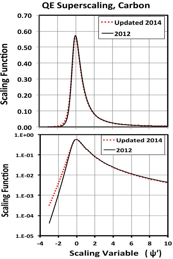
Fig. 3 shows two parametrizations of superscaling functions extracted from quasielastic electron scattering data on . Shown is the superscaling distribution extracted from a fit to electron scattering data used by Bosted and Mamyan [10] (solid black line labeled as 2012), and the superscaling function extracted from a recent updated fit[11] to data from a large number of quasielastic electron scattering experiments on (dotted red line labeled as 2014). The panel on top shows the superscaling functions on a a linear scale and the panel on the bottom shows the same superscaling functions on a logarithmic scale.
The 2014 superscaling function is given by:
| (2) |
The 2012 superscaling function is given by:
| (3) |
For both the 2012 and 2014 parametrizations the values of the Fermi motion parameter and energy shift parameter (given in Table 1) are taken from ref. [10].
The superscaling function is extracted from the longitudinal QE cross section for GeV2 where there are no Pauli blocking effects. At very low values of , the QE differential cross sections predicted by the superscaling should be multiplied by a Pauli blocking factor which reduces the predicted cross sections at low . The Pauli suppression factor (see Fig. 20) is given[10] by the function
| (4) |
For , otherwise no Pauli suppression correction is made. Here is the absolute magnitude of the momentum transfer to the target nucleus,
In this paper we show that the normalized differential quasielastic cross section predicted by the superscaling formalism can be well described by predictions of a modified effective spectral function (ESF). The parameters of the ESF are obtained by requiring that the ESF predictions for at values of 0.1, 0.3, 0.5 and 0.7 GeV2 be in agreement with the predictions of the 2014 superscaling function given in eq. 3.
The predictions of the formalism are given by
where N the integral of over all values of (for a given value of ).
| (GeV) | (GeV) | |
|---|---|---|
| 2 | 0.100 | 0.001 |
| 3 | 0.115 | 0.001 |
| 0.190 | 0.017 | |
| 0.228 | 0.0165 | |
| 0.230 | 0.023 | |
| 0.236 | 0.018 | |
| 0.241 | 0.028 | |
| 0.241 | 0.023 | |
| 0.245 | 0.018 |
1.4 Comparison of models for quasielastic scattering
For electron scattering, the nuclear response function is extracted from the normalized longitudinal differential cross section at a fixed vale of (). Here is the integral of for a fixed value of . The normalization removes the effects of the -dependent nucleon vector form factors. In models which assume scattering from independent nucleons, the response functions for the longitudinal and transverse QE cross sections are the same.
For neutrino scattering at high energy, the QE cross section is dominated by the structure function . Therefore, in models which assume scattering from independent nucleons the normalized cross section () at a fixed value of and high neutrino energy is also equal to the nuclear response function. For the neutrino case, the normalization removes the effects of the -dependent nucleon vector and axial form factors. Fig. 4 shows predictions for the normalized QE differential cross sections for 10 GeV neutrinos on at =0.5 GeV2 for various spectral functions. Here is plotted versus . The prediction of the superscaling formalism for is shown as the solid black line. The solid green line is the prediction using the ”Global Fermi” gas [7] momentum distribution given in Appendix B (eq. 33). The solid red line is the prediction using the Local Thomas Fermi gas (LTF) momentum distribution. The dotted purple line is the NuWro prediction using the full two dimensional Benhar-Fantoni[8] spectral function. The predictions of all of these spectral functions for are in disagreement with the predictions of the superscaling formalism.
2 Effective Spectral Function for
2.1 Momentum Distribution
The probability distribution for a nucleon to have a momentum in the nucleus is defined as
For GeV, we parametrize[13] by the following function:
| (5) |
where
For GeV we set = 0. Here, , is in GeV, N is a normalization factor to normalize the integral of the momentum distribution from =0 to =0.65 GeV to 1.0, and P() is in units of GeV-1. The parameters that describe the projected momentum distribution[13] for the Benhar-Fantoni[8] spectral function for nucleons bound in are given in the second column of table 2.
| Parameter | Benhar-Fantoni | ESF | ESF |
|---|---|---|---|
| Nucleus | |||
| (MeV) | 2Dspectral | 12.5 | 0.13 |
| 2Dspectral | 0.808 | 0 | |
| 2Dspectral | 0.192 | 1.00 | |
| 1.7 | 2.12 | 0.413475 | |
| 1.77 | 0.7366 | 1.75629 | |
| 1.5 | 12.94 | 8.29029 | |
| 0.8 | 10.62 | 3.621 x10⁻³ | |
| 2.823397 | 197.0 | 0.186987 | |
| 7.225905 | 9.94 | 6.24155 | |
| 0.00861524 | 4.36 x10⁻⁵ | 2.082 x10⁻⁴ | |
| 0.985 | 29.64 | 10.33 |

2.2 Removal Energy
The kinematics for neutrino charged current quasielastic scattering from a off-shell bound neutron with momentum and energy are given by:
| (6) | |||||
| (7) |
For scattering from a single off-shell nucleon, the term multiplying in Equations 6, 8 and 9 (and also Equations 21, 22, and 23) should be 1.0. However, we find that in order to make the spectral function predictions agree with superscaling at very low (e.g. ) we need to apply a -dependent correction to reduce the removal energy, e.g. due to final state interaction (of the first kind) at low . This factor is given in equation 7 and plotted in Fig. 7.
The value of the parameter =12.04 GeV-2 was extracted from the fits discussed in section 2.2.4. As mentioned earlier, is the momentum transfer to the neutron. We define the component of the initial neutron momentum which is parallel to as . The expression for depends on the process and is given by Equations 8 and 9 for the 1p1h, and 2p2h process, respectively.
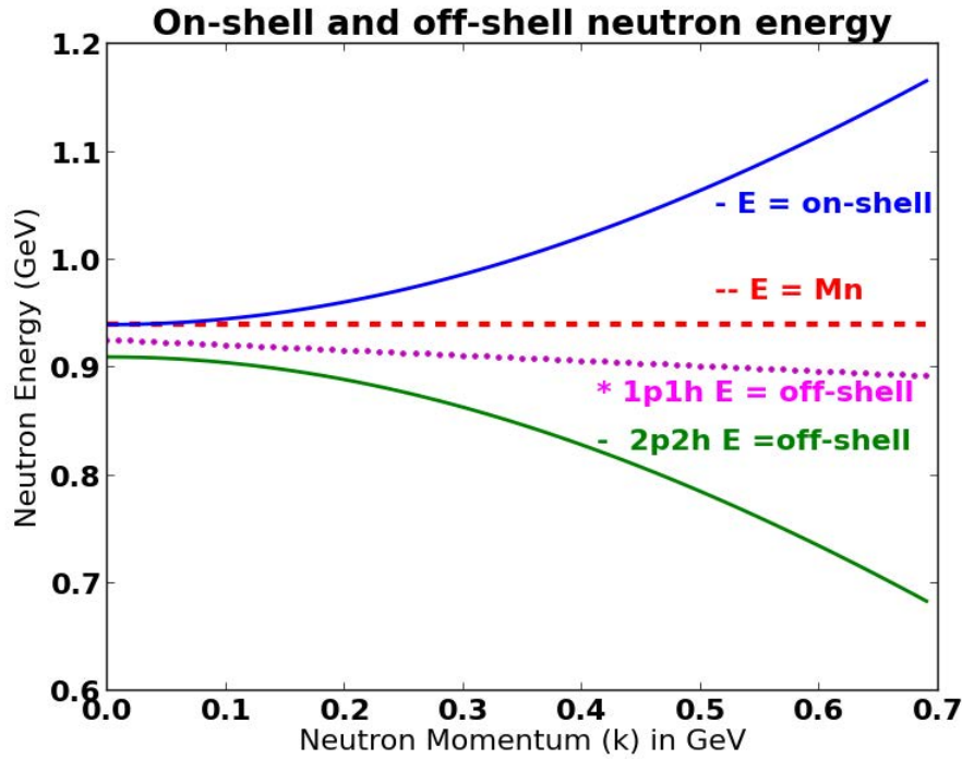
We assume that the off-shell energy () for a bound neutron with momentum can only take two possible values[12]. We refer to the first possibility as the 1p1h process (one proton, one hole in the final state). The second possibility is the 2p2h process(two protons and two holes in the final state).
In our effective spectral function model the 1p1h process occurs with probability , and the 2p2h process occurs with probability of . For simplicity, we assume that the probability is independent of the momentum of the bound nucleon.
2.2.1 The 1p1h process
The 1p1h process refers to scattering from an independent neutron in the nucleus resulting in a final state proton and a hole in the spectator nucleus. Fig. 1 illustrates the 1p1h process (for GeV2), for the scattering from an off-shell bound neutron of momentum in a nucleus of mass A[12]. In the 1p1h process, momentum is balanced by an on-shell recoil nucleus which has momentum and an average binding energy parameter , where . The initial state off-shell neutron has energy which is given by:
| (8) | |||||
The final state includes a proton and an nucleus which is in an excited state because the removal of the nucleon leaves hole in the energy levels of the nucleus.
For the 1p1h process, the removal energy of a nucleon includes the following two contributions:
- •
The binding energy parameter where .
- •
The kinetic energy of the recoil spectator nucleus .
2.2.2 The 2p2h process
In general, there are are several processes which result in two (or more) nucleons and a spectator excited nucleus with two (or more) holes in final state:
- •
Two nucleon correlations in initial state (quasi deuteron) which are often referred to as short range correlations (SRC).
- •
Final state interaction (of the first kind) resulting in a larger energy transfer to the hadronic final state (as modeled by superscaling).
- •
Enhancement of the transverse cross sections (”Transverse Enhancement”) from meson exchange currents (MEC) and isobar excitation.
In the effective spectral function approach the lepton energy spectrum for all three processes is modeled as originating from the two nucleon correlation process. This accounts for the additional energy shift resulting from the removal of two nucleons from the nucleus.
Fig. 5 illustrates the 2p2h process for scattering from an off-shell bound neutron of momentum (for GeV2). The momentum of the interacting nucleon in the initial state is balanced by a single on-shell correlated recoil nucleon which has momentum . The spectator nucleus is left with two holes. The initial state off-shell neutron has energy which is given by:
| (9) |
where is given by eq. 7.
For the 2p2h process, the removal energy of a nucleon includes the following two contributions:
- •
The binding energy parameter where .
- •
The kinetic energy of the recoil spectator nucleon given by .
Fig. 6 shows a comparison of the total energy for on-shell and off-shell bound neutrons in as a function of neutron momentum k (for GeV2 where V1.0). The energy for an unbound on-shell neutron is . The off-shell energy of a bound neutron is shown for both the 1p1h () and the 2p2h process ().
In the effective spectral function approach, all effects of final state interaction (of the first kind) are absorbed in the initial state effective spectral function. The parameters of the effective spectral function are obtained by finding the parameters , , , , , , , , , and for which the predictions of the effective spectral function best describe the predictions of the superscaling formalism for at values of 0.1, 0.3, 0.5 and 0.7 GeV2.
Fig. 8 compares predictions for for as a function of at =0.5 GeV2. The prediction of the effective spectral function is the dashed blue curve. The prediction of the superscaling model is the solid black curve. For =0.5 GeV2 the prediction of the effective spectral function is almost identical to the prediction of superscaling. All of the prediction for the effective spectral function are calculated from equation in Appendix B.
For the 2p2h process, each of the two final state nucleons can also undergo final state interactions (of the second kind) with other nucleons in the spectator nucleus.


2.2.3 Comparison of the 1p1h and 2p2h contributions
The top panel of Fig. 9 shows the prediction of the effective spectral function model for for QE scattering from a nucleus at = 0.5 GeV2, assuming that only the 1p1h process contributes. The bottom panel of Fig. 9 shows the prediction of the effective spectral function model for for QE scattering from a nucleus at = 0.5 GeV2 assuming that only the 2p2h process contributes.
We find that the effective spectral function with only the 1p1h process provides a reasonable description of the prediction of superscaling. Including a contribution from the 2p2h process in the fit improves the agreement and results in a prediction which is almost identical to the prediction of superscaling.
For reference, figures 9- 12 also show the prediction for the Fermi Gas model in blue, and the predictions from the Bodek-Ritchie[12] Fermi gas model which includes a high momentum contribution from two nucleon correlations in green. These predictions are calculated for 10 GeV neutrinos using the the GENIE neutrino Monte Carlo generator.
2.2.4 Comparisons as a function of for GeV2
Fig. 10 and Fig. 11 shows a comparison of the prediction of the effective spectral function for for to the predictions of the superscaling formalism for values of 0.3, 0.5, 0.7, 1.0, 1.2, 1.5 and 2.0 and GeV2.
In principle, it should not be possible for a spectral function approach to exactly reproduce superscaling at all values of . Nonetheless, the parameters which we optimized for values of 0.3, 0.5 and 0.7 GeV2 also provide a good description of for values of 1.0, 1.2, 1.5 and 2.0 GeV2.
2.2.5 Comparisons as a function of for GeV2
The low suppression factor of the removal energy which is given in eq. 7 is introduced in order to reproduce predictions of the superscaling model at GeV2.
Fig. 12 shows a comparison of the prediction for the shape () of the quasielastic peak for from the effective spectral function (red) to the predictions of the superscaling model (black). The predictions are shown as a function of for = 0.1 GeV2. The top panel show the predictions without the low correction factor to the removal energy. The bottom panel shows the predictions including the low correction factor to the removal energy, e.g. from final state interaction (of the first kind) at low .
Also shown (for reference) is the prediction for superscaling in black, the prediction for the Fermi Gas model in blue, and the predictions from the Bodek-Ritchie[12] Fermi gas model which includes a high momentum contribution from two nucleon correlations in green.
3 Spectral functions for other nuclei
Fig. 13 shows the predictions for the shape of the quasielastic peak () from the best fit effective spectral function (top panel) as compared to the predictions of superscaling model (bottom panel) for different nuclei. The predictions are shown as a function of for =0.5 GeV Fig. 14 shows the momentum distribution of the effective spectral function for various nuclei, and Table 3 gives the parameterizations of the effective spectral function for various nuclei.
| Parameter | ||||||||
|---|---|---|---|---|---|---|---|---|
| (MeV) | 5.3 | 14.0 | 12.5 | 16.6 | 12.5 | 20.6 | 15.1 | 18.8 |
| 0.312 | 0.791 | 0.808 | 0.765 | 0.774 | 0.809 | 0.822 | 0.896 | |
| 3.06 | 2.14 | 2.12 | 1.82 | 1.73 | 1.67 | 1.79 | 1.52 | |
| 0.902 | 0.775 | 0.7366 | 0.610 | 0.621 | 0.615 | 0.597 | 0.585 | |
| 10.93 | 9.73 | 12.94 | 6.81 | 7.20 | 8.54 | 7.10 | 11.24 | |
| 6.03 | 7.57 | 10.62 | 6.08 | 6.73 | 8.62 | 6.26 | 13.33 | |
| 199.6 | 183.4 | 197.0 | 25.9 | 21.0 | 200.0 | 18.37 | 174.4 | |
| 1.92 | 5.53 | 9.94 | 0.59 | 0.59 | 6.25 | 0.505 | 5.29 | |
| 5.26x10⁻⁵ | 59.0x10⁻⁵ | 4.36 x10⁻⁵ | 221. x10-5 | 121.5 x10⁻⁵ | 269.0x10⁻⁵ | 141.0 x10⁻⁵ | 9.28x10⁻⁵ | |
| 6.1 | 18.94 | 29.64 | 4.507 | 4.065 | 40.1 | 3.645 | 37.96 |


4 Transverse Enhancement and multi nucleon processes
Both spectral functions and the superscaling formalism model QE scattering in terms of scattering from independent nucleons in the initial state. The independent nucleon approach works well in modeling the longitudinal (electric) cross section for QE electron scattering from nuclear targets. However, it is known that none of the independent nucleon models can describe the transverse (magnetic) part of the QE electron scattering cross section. The transverse cross section is larger than the predictions of the independent nucleon model, and the enhancement is a function of . This experimental observation is usually referred to as ”Transverse Enhancement” (TE).
TE has been attributed to multi nucleon processes such as meson exchange currents and isobar excitation. There are two ways to account for these multi nucleon effects.
4.1 Accounting for contributions from multi nucleon processes
One way to account for TE is to use specific theoretical models to estimate the contributions from various multi nucleon processes such as meson exchange currents and isobar excitation. The differences between various model may provide an indication of the uncertainties of the calculations.
4.2 The Transverse Enhancement (TE) model
Another way to account for transverse enhancement is to parameterize the experimentally observed excess in the electron scattering data in a model independent way. In the TE model [19] this is done by modifying the magnetic form factors for bound nucleons.
As was done in reference [19], we have re-extracted the integrated transverse enhancement ratio , where
from electron scattering data from the JUPITER collaboration[21]. Here is the experimentally observed integrated transverse QE cross section and is the integrated transverse QE cross section predicted by super scaling.
Fig. 15 shows experimental values of as a function of . The black points are extracted from Carlson [20], and the higher are re-extracted from QE data from the JUPITER collaboration[21]. The dependence of is parametrized by the expression:
with A=5.194 and B=0.376 GeV2. The electron scattering data indicate that the transverse enhancement is maximal near =0.3 GeV2 and is small for greater than 1.5 GeV2 This parametrization is valid for carbon (A=12) (it is also an approximate representation for higher A nuclei).
We assume that the enhancement in the transverse QE cross section can be described by a modification of for nucleons bound in carbon, where and are the magnetic form factor of the proton and neutron, respectively (as measured in electron scattering experiments). We use the parametrization of to modify and for bound nucleons as follows.
| (10) |
Transverse enhancement increases the overall neutrino and antineutrino cross sections and changes the shape of the differential cross section as a function of as shown in the bottom panel of Fig. 15.
Fig. 16 shows the neutrino and antineutrino QE cross sections on with TE and without TE as a function of neutrino energy. The cross section for neutrinos is shown on the top panel and the cross section for antineutrinos is shown in bottom panel. Fig. 17 shows the ratio of the neutrino and antineutrino QE cross sections on with TE to the sum of free nucleon cross sections as a function of energy. The ratio for neutrinos is shown in the top panel and the ratio for antineutrinos is shown inn the bottom panel. On average the overall cross section is increased by about 18%.
Note that TE is a 2p2h process. Therefore, when TE is included in the model prediction, the relative fractions of the 1p1h and 2p2h should be changed as follows:
| (11) |
In the above prescription, the energy sharing between the two nucleons in the final state for the 2p2h TE process is the same as for the 2p2h process from short range two nucleon correlations. We can make other assumptions about the energy sharing between the two nucleus for the TE process. For example one can chose to use a uniform angular distribution of the two nucleons in the center of mass of the two nucleons as is done in NuWro[5]. This can easily be done in a neutrino MC event generator, since once the events are generated, one can add an additional step and change the energy sharing between the two nucleons.
In summary, we extract the TE contribution by taking the difference between electron scattering data and the predictions of the formalism for QE scattering. Therefore, predictions using ESF for QE with the inclusion of the TE contribution fully describe electron scattering data by construction.
Including the TE model in neutrino Monte Carlo generators is relatively simple. The first step is to modify the magnetic form factors for the proton and neutron as given in equation 10. This accounts for the increase in the integrated QE cross section. The second step is to change the relative faction of the 1p1h and 2p2h process as given in equation 11, which changes shape of the QE distribution in .
The effective spectral function model and the TE model are not coupled. One can use the effective spectral function to describe the scattering from independent nucleons, and use another theoretical model to account for the additional contribution from multi nucleon process. Alternatively, one can use an alternative model for the scattering from independent nucleons and use the TE model to account for the additional contribution from multi nucleon processes.
5 Effective spectral functions for deuterium
Neutrino charged current QE cross sections for deuterium are not modeled in current neutrino Monte Carlo generators. We find that neutrino interactions on deuterium can also be modeled with an effective spectral function.
We use the theoretical calculations of reference [14] to predict the shape of the transverse differential cross section () for deuterium at several values of as a function of = . These theoretical calculations are in agreement with electron scattering data. We tune the parameters of the effective spectral function to reproduce the spectra predicted by the theoretical calculations of reference [14].
Fig. 18 shows comparisons of model predictions for for QE electron scattering on deuterium as a function of = at =0.5 GeV2. The solid black line is the prediction from reference[14]. The red line is the prediction of the best fit parameters for the effective spectral function for deuterium. For comparison we also show (in blue) the prediction for a Fermi gas model with Fermi momentum = 0.100 GeV.
For reference, we note that the current default version of GENIE cannot be used nuclei with atomic weight . This is because GENIE = 0.169 GeV (which has been extracted by Moniz[7] for ) for all nuclei which have atomic weight . GENIE with the implementation of the effective spectral function can be used for all nuclei. Recently, the effective spectral function has been implemented as an option in private versions of NEUT[22] and GENIE[23].
The best fit parameters for the effective spectral function for deuterium are given in Table 2. For deuterium, the 2p2h process is the only process that can happen.
6 Pauli suppression
The Pauli suppression in deuterium is smaller than the Pauli suppression in heavier nuclei. The multiplicative Pauli suppression factor for deuterium has been calculated by S. K. Singh [15]. can be parametrized[16] by the following function.
| (12) |
where, A=0.588918, B=-17.2306, C= 0.749157. A comparison of the Pauli suppression factors for (eq. 4) and deuterium (eq. 12) is shown in Fig. 20.
7 Conclusion
We present parameters for an effective spectral function that reproduce the prediction for from the best currently available models for charged current QE scattering on nuclear targets. We present parameters for a large number of nuclear targets from deuterium to lead.
Since most of the currently available neutrino MC event generators model neutrino scattering in terms of spectral functions, the effective spectral function can easily be implemented. For example, it has taken only a few days to implement the effective spectral function as an option in recent private versions of NEUT[22] and GENIE[23].
The predictions using ESF for QE with the inclusion of the TE contribution fully describe electron scattering data by construction.
8 Acknowledgments
We thank Tomasz Golan for providing us with the predictions of NuWro, and Callum D. Wilkinson for implementation of the effective spectral function in NEUT.
9 Appendix A: Fermi smearing in the resonance region
9.1 The method of Bosted and Mamyan
Bosted and Mamyan[10] model Fermi motion effects for electron scattering data in the resonance and deep inelastic region by smearing the structure function on free nucleons to obtain the Fermi smeared structure function . The smearing is done over (which is the square of the mass of the hadronic final state) at fixed values of . Bosted and Mamyan[10] use the following prescription.
| (13) | |||||
where the sum approximates an integral. Here, and are the free proton [18] and neutron [17] structure functions.
The shifted values are defined as
| (14) |
where , and is the energy shift parameter. In the sum they use 99 values of
| (15) |
In the above equation is the normalized probability for a nucleon to have a fractional longitudinal momentum . Bosted and Mamyan use the following normalized Gaussian for the probability.
| (16) |
which is equivalent to
| (17) |
The sum is a step-wise integration over a Gaussian whose width is controlled by a Fermi momentum , truncated at ( ranges from -3 to +3), with a shift in central related to the energy shift parameter . The values of and used for the different nuclei are given in Table 1.
| Parameter | |||||||||
|---|---|---|---|---|---|---|---|---|---|
| (MeV) | 0.13 | 5.3 | 14.0 | 12.5 | 16.6 | 12.5 | 20.6 | 15.1 | 18.8 |
| 0 | 0.312 | 0.791 | 0.808 | 0.765 | 0.774 | 0.809 | 0.822 | 0.896 | |
| 0.2181 | 0.2560 | 0.1325 | 0.03819 | 0.1063 | 0.1063 | 0.1019 | 0.07645 | 0.1474 | |
| 0.6402 | 0.4343 | 0.3818 | 0.4168 | 0.3443 | 0.3443 | 0.3529 | 0.3892 | 0.3366 | |
| 0.4465 | 0.7321 | 0.5724 | 0.3688 | 0.5538 | 0.5538 | 0.5401 | 0.5049 | 0.5964 | |
| 0.9920 | 1.459 | 1.054 | 0.910 | 0.9555 | 1.008 | 0.9416 | 0.9356 | 0.9792 | |
| 3.233 | 3.126 | 2.122 | 1.928 | 1.870 | 1.935 | 1.873 | 1.889 | 1.900 | |
| (GeV) | 0.100 | 0.115 | 0.190 | 0.228 | 0.230 | 0.236 | 0.241 | 0.241 | 0.245 |
| 97.79 | 27.87 | 0 15.07 | 11.02 | 15.18 | 14.18 | 13.50 | 14.14 | 13.96 | |
| -0.2351 | 0.8118 | 0.6972 | 0.6772 | 0.5387 | 0.5466 | 0.5471 | 0.5252 | 0.5131 | |
| 96.24 | 22.53 | 11.18 | 7.770 | 11.66 | 10.74 | 10.15 | 10.78 | 10.72 | |
| 43.34 | 15.54 | 8.692 | 5.441 | 8.482 | 8.001 | 7.169 | 7.536 | 7.086 |
9.2 Fermi smearing in the resonance region using the effective spectral function
We have calculated the probability for the effective spectral function () for . The top panel of Fig. 21 shows the probability distributions plotted versus the variable for the effective spectral function as compared to the distribution used by Bosted and Mamyan. Also shown is the probability distribution for the Fermi Gas model with =0.228. The effective spectral function extends to higher momentum. In order to implement the effective spectral function we have fit to a sum of three normal Gaussians with zero mean and different standard deviations , and fractions , and .
| (18) | |||||
where , , , , and . For smearing with the distribution of the effective spectral function we also use a 99 step integration in where,
| (19) | |||||
Here, the sum is a step-wise integration over a Gaussian whose width is controlled by a Fermi momentum , truncated at ( ranges from -6 to +6), with a shift in central related to removal energy. The values of used for the different nuclei are given in Table 1.
Bosted and Mamyan calculate the shifted values of (equation 14) using a fixed value for the energy shift . Instead, we calculate the shifted values of (equation 21) using the off-shell neutron energies () for the 1p1h (eq. 22) and 2p2h (eq. 22) processes, respectively. In order calculate the -dependent off-shell neutrino energies we need to find the average as a function of .
The bottom panel of Fig. 21 shows the average value of the square of nucleon moment versus the square of its component () calculated for the effective spectral function for . What is shown specifically is as a function of . We parameterize by the following function:
| (20) |
We repeat the analysis for all other nuclei. The top panel of Fig. 22 shows ) for light nuclei. The middle panel shows ) for heavy nuclei, and the bottom panel shows the mean as a function of presented as as versus ().
The parameters for nuclei from to are given in Table 4. However, we note that aside from (deuterium) and , the functions for all nuclei are very similar. Therefore, as a good approximation, the parameters for can be used for all nuclei above A=12, and also for (provided that the appropriate Fermi momentum for each nucleus as given in Table 4 is used for each nucleus).
Smearing with the effective spectral function requires that the shifted value of are different for the the 1p1h and 2p2h contributions.
Therefore,
| (21) | |||||
Here is given by equation 20.
As mentioned earlier, the term multiplying in Equations 6, 8, 9, 21, 22, and 23 should be 1.0. However, we find that in order to make the spectral function agree with superscaling at very low (e.g. GeV2) we need to apply a -dependent correction of the form where =12.04 GeV-2. This term, shown in Fig. 7, accounts for the final state interaction (of the first kind) at low .
For the 1p1h process is given by equation 8, which when plugged into equation 21 for yields the following expression:
| (22) | |||||
For the 2p2h process is given by equation 9 which when plugged into equation 21 for yields the following expression:
| (23) | |||||
When smearing the proton and neutron structure functions, the 1p1h and 2p2h processes are weighted by the relative fractions given in Table 4.
Fig. 23 shows the results of Fermi motion smearing in ( GeV) of the free nucleon cross sections in the resonance region using the effective spectral function. The results are shown for several values of and compared to the Fermi motion smearing used by Bosted and Mamyan. The spectra smeared with the effective spectral function are are shifter to higher values of .
10 Appendix B: Calculation of the shape of the quasielastic peak
We calculate the shape of the quasielastic peak at fixed using the expressions below. The on-shell elastic structure function for the scattering of neutrinos on free neutrons[19] is given by
| (24) |
where is given in terms of vector and axial form factors.
| (25) | |||
| (26) |
From conserved vector current (CVC) and are related to the electron scattering electromagnetic form factors[24] , , , and :
The axial form factor can be approximated by the dipole form
Where , and GeV[24]. Fits that include modifications to dipole form for both vector and axial form factors can be found in Ref.[24].
We note that when we calculate the shape of the QE peak at fixed the function cancels out.
For the scattering from an off-shell nucleon, the energy conservation function takes the following form:
| (27) |
where . Here is the angle between the direction of the momentum transfer and . The shape of the quasielastic peak at fixed is then given by
Where is the probability distribution for a nucleon to have a momentum in the nucleus. For all of the momentum distributions that we investigate we set the probability to zero for where =0.65 GeV.
10.1 The shape of the quasielastic peak for the Fermi gas model
For the Fermi gas model we can get an approximate distribution for in closed form. We use this calculation as a check on our results which are obtained using equation .
For the Fermi gas model we do the calculation in cylindrical coordinate
Equation can then be written as
| (29) |
For the Fermi gas model the momentum distribution is zero for , and for it is given by
| (30) |
For simplicity, we assume that the energy of the off shell neutron is a constant which is independent of k. Using we obtain
| (31) |
| (32) | |||||
Integrating the function in equation 27 over we get
| (33) |
The above equation satisfies the normalization condition
References
- (1) C. Andreopoulos [GENIE Collaboration], Acta Phys. Polon. B 40, 2461(2009), C.Andreopoulos (GENIE), Nucl. Instrum. Meth.A614, 87,2010.
- (2) H. Gallagher, (NEUGEN) Nucl. Phys. Proc. Suppl. 112 (2002).
- (3) Y. Hayato (NEUT), Nucl Phys. Proc. Suppl.. 112, 171 (2002).
- (4) D. Casper (NUANCE) , Nucl. Phys. Proc. Suppl. 112, 161 (2002) (http://nuint.ps.uci.edu/nuance/).
- (5) J. Sobczyk (NuWro), PoS NUFACT 08, 141 (2008), C. Juszczak, Acta Phys. Polon. B40 (2009) 2507 (http://borg.ift.uni.wroc.pl/nuwro/).
- (6) T. Leitner, O. Buss, L. Alvarez-Ruso, U. Mosel (GiBUU), Phys. Rev. C79, 034601 (2009) (arXiv:0812.0587).
- (7) E. J. Moniz et al. Phys. Rev. Lett. 26, 445(1971); E. J. Moniz, Phys. Rev. 184, 1154 (1969); R. A. Smith and E. J. Moniz, Nucl. Phys. B43, 605 (1972).
- (8) O. Benhar and S. Fantoni and G. Lykasov, Eur Phys. J. A 7 (2000), 3, 415; O, Benhar et al., Phys. Rev. C55. 244 (1997).
- (9) J.E. Amaro, M.B. Barbaro, J.A. Caballero, T.W. Donnelly, A. Molinari, and I. Sick, Phys. Rev. C 71, 015501 (2005). arXiv:nucl-th/0409078.
- (10) P. E. Bosted, V. Mamyan, arXiv:1203.2262.
- (11) M. E. Christy, private communication (2014).
- (12) A. Bodek, and J. L. Ritchie, Phys. Rev. D23, 1070 (1980). A. Bodek and J. L. Ritchie, Phys. Rev. D24, 1400 (1981).
- (13) S. Mishra, (NOMAD collaboration) private communication, fit parameters from E. Iacopini (1997).
- (14) M. E. Christy, N. Kalantarians, J. J. Ethier, and W. Melnitchouk. In preparation (2014).
- (15) S.K. Singh, Nucl. Phys. B36 419(1972);.K. Singh and H. Arenhove,
- (16) H. Budd, A. Bodek, J. Arrington, Nucl.Phys.Proc.Suppl. 139, 90(2005), Z. Phys. A 324, 3476 (1986).
- (17) P.E. Bosted and M.E. Christy, Phys. Rev. C 77, 065206 (2008). (arXiv:0711.0159).
- (18) M.E. Christy and P.E. Bosted, Phys. Rev. C 81, 055213 (2010). (arXiv:0712.3731).
- (19) A. Bodek, H. S. Budd and M. E. Christy, Eur. Phys. J. C 71, 1726 (2011).
- (20) J. Carlson, J. Jourdan, R. Schiavilla, I. Sick, Phys.Rev. C65, 024002 (2002).
- (21) A. Bodek, C.Keppel and M. E. Christy (spokespersons JUPITER Collaboration), Jefferson Lab Experiment E04-001.
- (22) Callum D. Wilkinson, private communication (NEUT).
- (23) Brian Coopersmith, private communication (GENIE).
- (24) A. Bodek, S. Avvakumov, R. Bradford, and H. Budd, Eur. Phys. J. C53, 349 (2008).