Simultaneous Finite Automata:
An Efficient Data-Parallel Model
for Regular Expression Matching

Ryoma Sin’ya Affiliation: Department of Mathematical
and Computing Sciences,
Tokyo Institute of Technology
Email: shinya.r.aa@m.titech.ac.jp Kiminori Matsuzaki Affiliation: School of Information,
Kochi University of Technology
Email: matsuzaki.kiminori@kochi-tech.ac.jp Masataka Sassa Affiliation: Department of Mathematical
and Computing Sciences,
Tokyo Institute of Technology
Email: sassa@is.titech.ac.jp

Abstract

Automata play important roles in wide area of computing and the growth of multicores calls for their efficient parallel implementation. Though it is known in theory that we can perform the computation of a finite automaton in parallel by simulating transitions, its implementation has a large overhead due to the simulation. In this paper we propose a new automaton called simultaneous finite automaton (SFA) for efficient parallel computation of an automaton. The key idea is to extend an automaton so that it involves the simulation of transitions. Since an SFA itself has a good property of parallelism, we can develop easily a parallel implementation without overheads. We have implemented a regular expression matcher based on SFA, and it has achieved over 10-times speedups on an environment with dual hexa-core CPUs in a typical case.

This paper has been accepted at the following conference: 2013 International Conference on Parallel Processing (ICPP-2013), October 1-4, 2013 Ecole Normale Supérieure de Lyon, Lyon, France.

I Introduction

Automata play important roles in theory and practice in a wide area of computing. For example the use of non-deterministic or deterministic automata is crucial in regular expression matching. Under the growth of multicores, parallelism becomes more and more important. In previous studies [1, 2], computations of automata are naively executed in parallel when both/either of queries and/or data are multiple, while a single computation of an automaton is executed in sequential. To extract more parallelism, parallelizing an automaton itself would be important. It has been known for a long time in theory that we can perform the computation of a finite-state automaton in parallel [3, 4]. The basic idea of the parallelization is to simulate all the transitions from all the possible states speculatively. However, as reported in previous studies [5, 6, 7, 8], such a parallel implementation has a large overhead due to the speculative simulation.

In this paper, we propose a novel approach for parallelizing the computation of automata. The key idea is to extend automata so that they involve the speculative simulation from all the states. We develop new automata named simultaneous finite automata (SFA in short) as extensions of finite-state automata where the states in SFA are given as mappings from states to states of the original automata. The key property of the SFA is that they essentially involve parallelism and thus we can straightforwardly implement the computation of SFA in parallel. Though such an extension may increase the size of automata, we can remove the runtime overhead. It is worth noting that usually automata are considerably smaller than data and the runtime speedup outstrips the enlargement of automata.

We can systematically construct an SFA from either an NFA or a DFA by a technique similar to the so-called subset construction technique. In general, such a construction may increase the number of states exponentially. However, for widely-used regular expressions, the number of states in SFA is no more than the square of that in the original automata. We show the effectiveness of SFA with the experiment results of the SFA-based parallel regular expression matching. Our SFA-based implementation has almost no overhead and achieved over 10-times speedups on an environment with dual hexa-core CPUs with respect to the DFA-based sequential implementation in a typical case.

The contributions of this paper are summarized as follows.

•

We proposed a new automaton, simultaneous finite automaton, for parallel regular expression matching (Sect. IV). By using SFA, we can compute regular expression matching simply in parallel without overheads (Algorithm 5). This SFA-based parallel regular-expression matcher is available online [9].
•

We developed an algorithm for constructing SFA from NFA or DFA (Algorithm 4). Since the algorithm is a natural extension of the subset construction algorithm, we can apply known implementation techniques for it.
•

The only concern of SFA is the size explosion with respect to DFA or NFA. We show that almost all the SFA are small enough for practical regular expressions in the SNORT rulesets. We also discuss the cases that SFA have as many states as the upper bound.

The rest of the paper is organized as follows. We introduce the basic idea of automata in Sect. II, and we review the parallelization method based on the speculative simulation in Sect. III. In Sect. IV, we define the simultaneous finite automata and discuss their properties. In Sect. V, we develop the implementation of SFA: a construction method and an application to parallel regular expression matching. In Sect. VI, we show the experimental results on SFA’s size, scalability, and overheads. In Sect. VII, we discuss the algebraic characterization of SFA for the theoretical upper bound of the number of states. Finally, we conclude the paper in Sect. VIII.

Remarks on automata theory. Automata theory has been deeply studied for a long time and there exist many extended models of automata in terms of parallelism. Some examples are parallel finite automata [10], concurrent finite automata [11], and alternating finite automata [12]. These models are extension for dealing with parallel/concurrent events, and they are not for implementing parallel matching of an automaton. The SFA in this paper is a new automata for discussing data-parallel regular expression matching.

II Preliminaries

II-A Notation

In this paper, we describe definitions and algorithms with symbols in the basic set theory. Some things to note: $|A|$ denotes the size of set $A$ (number of their elements). $\mathfrak{P}(A)$ is the power set of $A$ and $|\mathfrak{P}(A)|=2^{|A|}$ holds. $\mathfrak{F}(A,B)$ denotes all the mappings from $A$ to $B$ ( $f:A\rightarrow B$ ) and $|\mathfrak{F}(A,B)|=|B|^{|A|}$ holds. In particular, $\mathfrak{F}(A,A)$ is called a transformation of $A$ , and $\mathfrak{F}(A,\mathfrak{P}(A))$ is called a correspondence of $A$ . We define function composition $\circ$ on transformations and correspondences as follows:

	$\displaystyle f,g\in\mathfrak{F}(A,A),\forall a\in A\;\;\;\;\;\;(f\circ g)(a)$	$\displaystyle:=$	$\displaystyle f(g(a)),$
	$\displaystyle f,g\in\mathfrak{F}(A,\mathfrak{P}(A)),\forall a\in A\;\;\;\;\;\;(f\circ g)(a)$	$\displaystyle:=$	$\displaystyle\bigcup_{b\in g(a)}f(b).$

We also define reverse composition $\bullet$ as $f\bullet g:=g\circ f$ . Here, note that function composition and reverse composition are always associative.

II-B Finite Automata

We briefly introduce some basics of automata theory according to [13]. First we give the definition of nondeterministic and deterministic finite automata.

Definition 1

A nondeterministic finite automaton (NFA) ${\cal N}$ is a quintuple ${\cal N}=(Q,\Sigma,\delta,I,F)$ , where $Q$ is a finite set of states, $\Sigma$ is a set of input symbols, $\delta$ is a transition function of type $Q\times\Sigma\rightarrow\mathfrak{P}(Q)$ , $I\subseteq Q$ is a set of initial states, and $F\subseteq Q$ is a set of final states. $\diamond$

Definition 2

A deterministic finite automaton (DFA) ${\cal D}$ is a special case of NFA, where $I$ and every image of $\delta$ are singletons:

$\displaystyle|I|=1\quad\land\quad\forall q\in Q,\forall\sigma\in\Sigma\left[|\delta(q,\sigma)|=1\right].$ $\diamond$

We may say the number of states in an automaton as the size of the automaton, and we denote the size of automaton ${\cal A}$ as $|{\cal A}|$ . We introduce $\widehat{\delta}$ for an extended transition function over input texts:

	$\displaystyle\widehat{\delta}(q,\sigma w)$	$\displaystyle:=$	$\displaystyle\bigcup_{q^{\prime}\in\delta(q,\sigma)}\widehat{\delta}(q^{\prime},w),$
	$\displaystyle\widehat{\delta}(q,\epsilon)$	$\displaystyle:=$	$\displaystyle\{q\}~\mbox{.}$

The symbol $\epsilon$ denotes empty word and transition over $\epsilon$ does nothing. We also introduce bound transition function $\delta^{\sigma},\widehat{\delta}^{w}:Q\rightarrow\mathfrak{P}(Q)$ defined by follows:

	$\displaystyle\delta^{\sigma}(q)$	$\displaystyle:=$	$\displaystyle\delta(q,\sigma),$
	$\displaystyle\widehat{\delta}^{w}(q)$	$\displaystyle:=$	$\displaystyle\widehat{\delta}(q,w)~\mbox{.}$

If $p\in\widehat{\delta}(q,w)$ is a transition of automaton $\cal{A}$ , $w$ is said to be the label of the transition and we will write $q\xrightarrow[\cal{A}]{w}p$ (or simply $q\xrightarrow{w}p$ if it is unambiguous).

Definition 3

A computation $c$ in ${\cal A}$ is a sequence of transitions, which can be written as follows:

c:=q_{0}\xrightarrow{\sigma_{1}}q_{1}\xrightarrow{\sigma_{2}}q_{2}\xrightarrow{\sigma_{3}}\cdots\xrightarrow{\sigma_{n}}q_{n}~\mbox{.}

A word in $\Sigma^{*}$ is accepted by ${\cal A}$ if it is the label of a computation that begins at an initial state and ends at a final state in ${\cal A}$ . $\diamond$

Definition 4

$L(\cal{A})$ denotes the set of all the words accepted by $\cal{A}$ :

$\displaystyle L({\cal A})=\left\{w~|~\exists q\in I,\exists p\in F\left[q\xrightarrow[\cal{A}]{w}p\right]\right\}.$ $\diamond$

We say two automata ${\cal A}$ and ${\cal A}^{\prime}$ are equivalent if $L({\cal A})=L({\cal A}^{\prime})$ holds. The following theorem shows that there exists an equivalent DFA to every automaton.

Theorem 1 (Rabin and Scott[14])

Every automaton $\cal{A}$ is equivalent to a DFA $\cal{D}$ . If $\cal{A}$ is finite with $n$ states, $\cal{D}$ can be constructed with at most $2^{n}$ states.

Proof:

Let ${\cal A}=(Q,\Sigma,\delta,I,F)$ be an automaton. We consider an automaton ${\cal D}=(Q_{d},\Sigma,\delta_{d},I_{d},F_{d})$ : $Q_{d}$ is $\mathfrak{P}(Q)$ ; $\delta_{d}$ is the additive extension of $\delta$

S\in\mathfrak{P}(Q),\sigma\in\Sigma\;\;\;\;\;\;\delta_{d}(S,\sigma):=\displaystyle\bigcup_{q\in S}\delta(q,\sigma)~\mbox{;}

$I_{d}$ is a singleton of set $\{I\}$ ; final states are given by $F_{d}=\{S\in\mathfrak{P}(Q)|S\cap F\neq\emptyset\}$ . The automaton ${\cal D}$ is deterministic. Furthermore, it is equivalent to ${\cal A}$ since we have the following series of equivalences:

$\displaystyle w\in L({\cal A})$	$\displaystyle\Leftrightarrow$	$\displaystyle\displaystyle\exists q\in I\left[\widehat{\delta}(q,w)\cap F\neq\emptyset\right]$
	$\displaystyle\Leftrightarrow$	$\displaystyle\widehat{\delta}_{d}(\{I\},w)\cap F\neq\emptyset$
	$\displaystyle\Leftrightarrow$	$\displaystyle\displaystyle\widehat{\delta}_{d}(I_{d},w)\in F_{d}\Leftrightarrow w\in L({\cal D}).$

$\Box$

II-C Subset Construction and Sequential Computation in DFA

It is often faster to perform the computation with DFA than to do with NFA. Given an NFA, we can determinize it by the subset construction technique shown in Algorithm 1. Starting from the set of initial states, we compute the accessible subset of DFA step by step considering only those states obtained by applying the transition function to the states already calculated.

Algorithm 1 Subset construction

0: Automata

{\cal A}=(Q,\Sigma,\delta,I,F)

0: DFA

{\cal D}=(Q_{d},\Sigma,\delta_{d},I_{d},F_{d})

is equivalent to

{\cal A}

Q_{d}\leftarrow\emptyset,Q_{tmp}\leftarrow\{I\}

2: while

Q_{tmp}\neq\emptyset

3: choose and remove a set

S

from

Q_{tmp}

Q_{d}\leftarrow Q_{d}\cup\{S\}

5: for all

\sigma\in\Sigma

S_{next}\leftarrow\bigcup_{q\in S}\delta(q,\sigma)

\delta_{d}[S,\sigma]\leftarrow S_{next}

8: if

S_{next}\notin Q_{d}

then

Q_{tmp}\leftarrow Q_{tmp}\cup\{S_{next}\}

9: end for

10: end while

11:

I_{d}\leftarrow\{I\}

12:

F_{d}\leftarrow\{S\in Q_{d}|S\cap F\neq\emptyset\}

Sequential implementation of the computation in DFA is straightforward. Algorithm 2 shows the sequential program for the computation in DFA, in which we use a table $\delta_{d}[q,\sigma]$ for the transition function. Note that we store only a single state and reuse it during the computation.

Algorithm 2 Sequential computation of DFA

0: DFA

{\cal D}=(Q_{d},\Sigma,\delta_{d},\{q_{0}\},F_{d})

, and word

w=\sigma_{1}\sigma_{2}\cdots\sigma_{n}

q_{final}

is the destination such that

q_{0}\xrightarrow[\cal D]{w}q_{final}

q\leftarrow q_{0}

2: for

i=1\to n

q\leftarrow\delta_{d}[q,\sigma_{i}]

q_{final}\leftarrow q

Let ${\cal D}$ be the DFA, $\Sigma$ be the set of input symbols, and $n$ be the size of input word. Then, the sequential computation in DFA takes $\mathrm{O}(n)$ time, and the number of elements in the table of the transition function is $\mathrm{O}(|{\cal D}||\Sigma|)$ .

III Prior Works: Parallel Computation in DFA with Speculative Simulation

It has been known for a long time that the computation in DFA can be performed in parallel on parallel random access machines (PRAMs) [3, 4]. The fundamental idea is the speculative simulation of transitions in which we consider all the states as initial states. Such simulation of transitions forms a finite-sized mapping (between sets of states) and composition of finite-sized mappings is associative. This associativity in the composition of mappings enables us to perform parallel reduction for the computation of DFA.

Algorithm 3 shows a parallel implementation of the computation of DFA based on speculative simulation [5, 6, 7, 8]. The following two points are important in this algorithm. First, the mappings $T_{i}[\,]$ are computed on subwords independently in parallel and they contain transitions from all the states. Secondly, we can reduce the subresults either in parallel with associative binary operator $\bullet$ or in sequential.

Algorithm 3 Parallel computation of DFA

0: DFA

{\cal D}=(Q_{d},\Sigma,\delta_{d},\{q_{0}\},F_{d})

, number of threads

p

,word

w=\sigma_{11}\cdots\sigma_{1m_{1}}\sigma_{21}\cdots\sigma_{2m_{2}}\cdots\sigma_{p1}\cdots\sigma_{pm_{p}}

q_{final}

is destination such that

q_{0}\xrightarrow[\cal D]{w}q_{final}

1: for all

i\in[1,2,\ldots,p]

parallel do

2: for all

q\in Q_{d}

T_{i}[q]\leftarrow q

4: for

j=1\to m_{i}

5: for all

q\in Q_{d}

T_{i}[q]\leftarrow\delta(T_{i}[q],\sigma_{ij})

7: end for

8: // parallel reduction // sequential reduction

T\leftarrow T_{1}\bullet T_{2}\bullet\ldots\bullet T_{p}

q_{final}\leftarrow q_{0}

10:

q_{final}\leftarrow T[q_{0}]

for

i=1\rightarrow p

11:

q_{final}\leftarrow T_{i}[q_{final}]

Let ${\cal D}$ be the DFA, $n$ be the size of input word, $p$ be the number of processors. The time complexities of Algorithm 3 are $\mathrm{O}(|{\cal D}|n/p+|{\cal D}|\log p)$ when parallel reduction is used or $\mathrm{O}(|{\cal D}|n/p+p)$ when sequential reduction is used [5]. The coefficient $|{\cal D}|$ comes from the speculative simulation of transitions, and it means that the parallel implementation no longer runs faster than the sequential implementation when the size of the DFA is large.

IV Simultaneous Finite Automata

The simulation-based parallel computation of DFA has a large overhead linear to the size of DFA. In this section, we propose a new model of automata that involve the simulation of transitions in the definition. The key idea is that we can evaluate the simulation in advance in the same way as we evaluate the set of transitions during the construction of DFA from NFA. The proposed model have a good property for data parallel computation.

IV-A Formal Definition

We call the automaton simultaneous finite automaton (SFA, in short). A state in SFA corresponds to a mapping from states to sets of states in the normal finite automata.

Definition 5

Let ${\cal A}=(Q,\Sigma,\delta,I,F)$ be an automaton. A simultaneous finite automaton (SFA) constructed from ${\cal A}$ is a quintuple $(Q_{s},\Sigma,\delta_{s},I_{s},F_{s})$ :

•

$Q_{s}\subseteq\mathfrak{F}(Q,\mathfrak{P}(Q))$ is a set of mappings;
•

$\Sigma$ is the same set of symbols as ${\cal A}$ ;
•

$\delta_{s}$ is the additive extension of $\delta$ in ${\cal A}$ that is defined as $f\in Q_{s},\sigma\in\Sigma,\;\;\delta_{s}(f,\sigma):=\{f\bullet\delta^{\sigma}\}\mbox{;}$
•

$I_{s}\subseteq Q_{s}$ is a singleton of identity mapping $\{f_{I}\}$ that satisfies $f_{I}(q)=\{q\}$ for any $q\in Q$ ;
•

$F_{s}\subseteq Q_{s}$ is defined as $F_{s}=\{f\in Q_{s}~|~\exists q\in I\penalty\left[f(q)\cap F\neq\emptyset\right]\}$ . $\diamond$

By definition, SFA are entirely deterministic. As described later, SFA can be regarded as DFA with simultaneity.

Theorem 2

Every automaton $\cal{A}$ is equivalent to an SFA $\cal{S}$ . If $\cal{A}$ is finite with $n$ states, $\cal{S}$ can be constructed with at most $2^{n^{2}}$ states. In particular, if ${\cal A}$ is deterministic, $\cal{S}$ can be constructed with at most $n^{n}$ states.

Proof:

Let the original automaton be ${\cal A}=(Q,\Sigma,\delta,I,F)$ , and the SFA constructed from ${\cal A}$ be ${\cal S}=(Q_{s},\Sigma,\delta_{s},\{f_{I}\},F_{s})$ .

In addition to the fact that ${\cal S}$ is deterministic, ${\cal S}$ is equivalent to ${\cal A}$ since we have the following series of equivalences:

$\displaystyle w\in L({\cal A})$	$\displaystyle\Leftrightarrow$	$\displaystyle\exists q\in I\left[\widehat{\delta}(q,w)\cap F\neq\emptyset\right]$
	$\displaystyle\Leftrightarrow$	$\displaystyle\exists q\in I\left[\widehat{\delta}_{s}(f_{I},w)(q)\cap F\neq\emptyset\right]$
	$\displaystyle\Leftrightarrow$	$\displaystyle\widehat{\delta}_{s}(f_{I},w)\in F_{s}\Leftrightarrow w\in L({\cal S}).$

The size of the set of mappings is bounded as $|Q_{s}|\leq|\mathfrak{F}(Q,\mathfrak{P}(Q))|=2^{|Q|^{2}}$ . If ${\cal A}$ is deterministic, transition function is one-to-one correspondence and $|Q_{s}|\leq|\mathfrak{F}(Q,Q)|=|Q|^{|Q|}$ . $\Box$

IV-B Example

Here we give an example of an SFA, which corresponds to a DFA. Notice that, though the states in SFA have meanings of mappings from states to sets of states in corresponding automaton, we need not to mind it when we compute the transitions in SFA. In other words, we can compute all the transitions in a finite automaton simultaneously by simply computing the transitions in SFA.

Example 1

Refer to caption — Fig. 1: ${\cal D}_{1}:L({\cal D}_{1})=L({\mathtt{(ab)*}})$

$f_{0}$	$f_{1}$	$f_{2}$	$f_{3}$	$f_{4}$	$f_{5}$
$0\mapsto\{0\}$	$0\mapsto\{1\}$	$0\mapsto\{2\}$	$0\mapsto\{2\}$	$0\mapsto\{0\}$	$0\mapsto\{2\}$
$1\mapsto\{1\}$	$1\mapsto\{2\}$	$1\mapsto\{0\}$	$1\mapsto\{2\}$	$1\mapsto\{2\}$	$1\mapsto\{1\}$
$2\mapsto\{2\}$	$2\mapsto\{2\}$	$2\mapsto\{2\}$	$2\mapsto\{2\}$	$2\mapsto\{2\}$	$2\mapsto\{2\}$

Figure I shows DFA ${\cal D}_{1}$ that accepts $L(\verb|(ab)*|)$ . Figure I shows SFA ${\cal S}_{1}$ equivalent to ${\cal D}_{1}$ where the states in ${\cal S}_{1}$ imply the mappings listed in Table I. Final states are denoted with doubled circles in these figures.

Consider the computation of ${\cal S}_{1}$ over abab. By following the states in Fig. I, we have transitions $f_{0}\xrightarrow[{\cal S}_{1}]{\mathtt{a}}f_{1}\xrightarrow[{\cal S}_{1}]{\mathtt{b}}f_{4}\xrightarrow[{\cal S}_{1}]{\mathtt{a}}f_{1}\xrightarrow[{\cal S}_{1}]{\mathtt{b}}f_{4}$ . Here, $f_{4}(0)=\{0\}$ implies $0\xrightarrow[{\cal D}_{1}]{\mathtt{abab}}0$ . Since the state $0$ is an accepted state in ${\cal D}_{1}$ , $f_{4}$ is also an accepted state in ${\cal S}_{1}$ . $\diamond$

IV-C Data-Parallel Property of SFA

We finally show an important property of SFA: the data-parallel nature in SFA. For any input text, we can divide it at any points and apply the computation of SFA in parallel.

Lemma 1

Let ${\cal S}$ be an SFA, $f$ be a state in ${\cal S}$ , $f_{w_{1}}$ and $f_{w_{2}}$ be the states satisfying $f\xrightarrow[{\cal S}]{w_{1}}f_{w_{1}}$ and $f_{I}\xrightarrow[{\cal S}]{w_{2}}f_{Iw_{2}}$ . Then the following equation holds:

\displaystyle f\xrightarrow[{\cal S}]{w_{1}w_{2}}f_{w_{1}w_{2}}\Leftrightarrow f_{w_{1}}\bullet f_{Iw_{2}}=f_{w_{1}w_{2}}~\mbox{.}

Proof:

By definition, we have

	$\displaystyle f\xrightarrow[{\cal S}]{w_{1}w_{2}}f_{w_{1}w_{2}}~\Leftrightarrow~\widehat{\delta}_{s}(f_{w_{1}},w_{2})=\{f_{w_{1}w_{2}}\}$		(1)
	$\displaystyle\;\;\;\;\;\;\mathop{\mathrm{where}}\nolimits\;\widehat{\delta}_{s}(f,w_{1})=\{f_{w_{1}}\}~\mbox{.}$

We can transform the left-hand side as follows by applying the definition of SFA.

	$\displaystyle\widehat{\delta}_{s}(f_{w_{1}},w_{2})$	$\displaystyle=$	$\displaystyle\{f_{w_{1}}\bullet\widehat{\delta}_{s}^{w_{2}}\}=\{f_{w_{1}}\bullet(f_{I}\bullet\widehat{\delta}_{s}^{w_{2}})\}$		(2)
		$\displaystyle=$	$\displaystyle\{f_{w_{1}}\bullet f_{Iw_{2}}\}.$		(2)

We used the fact that $f_{I}$ is an identity function and the equation $\delta_{s}(f_{I},w_{2})=\{f_{I}\bullet\widehat{\delta}_{s}^{w_{2}}\}=\{f_{Iw_{2}}\}$ . The lemma follows from Equations (1) and (2). $\Box$

This lemma enables us to introduce the following important theorem about the data-parallelism of the SFA.

Theorem 3

The computation in SFA $f_{I}\xrightarrow[{\cal S}]{w}f$ can be derived by any division of label $w=w_{1}w_{2}\ldots w_{n}$ .

Proof:

Computation $f_{I}\xrightarrow[{\cal S}]{w=w_{1}w_{2}\cdots w_{n}}f$ can be decomposed into the following equation by Lemma 1:

f=f_{w_{1}}\bullet f_{w_{2}}\bullet\cdots\bullet f_{w_{n}}\;\;\;\mathop{\mathrm{where}}\nolimits\;\;\;f_{I}\xrightarrow[{\cal S}]{w_{i}}f_{w_{i}}\;\;\;\;\;\;(i=1,\ldots,n)~\mbox{.}

Each computation $f_{I}\xrightarrow[{\cal S}]{w_{i}}f_{w_{i}}$ has no dependency on the other computations and these composition is associative. Hence, computation in SFA can be performed in a data-parallel manner. We call this method parallel computation in SFA. $\Box$

In the following of the paper, we may classify the SFA in terms of the original automaton. We call the SFA constructed from NFA as N-SFA, and that from DFA as D-SFA.

V Implementing SFA

V-A Construction of SFA from Finite Automaton

Algorithm 4 shows how we can construct an SFA from a finite automaton. We name the algorithm correspondence construction after the subset construction algorithm (Algorithm 1) that constructs a DFA from an NFA. The correspondence construction algorithm is very similar to the subset construction algorithm, and the main difference in line 6 of Algorithm 4: we compute a mapping $f_{next}(q)$ for all the states in the original automaton. If the original automaton is deterministic, then the image of the transition function is a singleton and we can simplify the line 6 as follows.

q\in Q\;\;\;\;\;f_{next}(q):=\delta(q^{\prime},\sigma)\;\mathop{\mathrm{where}}\nolimits\;\{q^{\prime}\}=f(q)\mbox{.}

Algorithm 4 Correspondence construction

0: Automaton

{\cal A}=(Q,\Sigma,\delta,I,F)

0: SFA

{\cal S}=(Q_{s},\Sigma,\delta_{s},I_{s},F_{s})

is equivalent to an automaton

{\cal A}

Q_{s}\leftarrow\emptyset,Q_{tmp}\leftarrow\{f_{I}\}

2: while

Q_{tmp}\neq\emptyset

3: choose and remove a mapping

f

from

Q_{tmp}

Q_{s}\leftarrow Q_{s}\cup\{f\}

5: for all

\sigma\in\Sigma

q\in Q\;\;\;f_{next}(q):=\bigcup_{q^{\prime}\in f(q)}\delta(q^{\prime},\sigma)

\delta_{s}[f,\sigma]\leftarrow f_{next}

8: if

f_{next}\notin Q_{s}

then

Q_{tmp}\leftarrow Q_{tmp}\cup\{f_{next}\}

9: end for

10: end while

11:

I_{s}\leftarrow\{f_{I}\}

12:

F_{s}\leftarrow\{f\in Q_{s}|\exists q\in I|f(q)\cap F\neq\emptyset\}

As is the case of the subset construction, the number of the states in the constructed SFA may increase exponentially compared with that in the original automaton. As we have stated in Theorem 2, in the worst case, from an NFA with $n$ states the number of the states in an N-SFA becomes $2^{n^{2}}$ , and from a DFA with $n$ states the number of the states in a D-SFA becomes $n^{n}$ . You might consider that these numbers of states dismiss the practical use, but it is not true. From DFA that correspond to typical regular expressions, fortunately, the number of states in the constructed D-SFA is no more than the square of that in DFA (we will show this fact in Sect. VI-A).

The on-the-fly construction is a well known technique [15] in the implementation of an advanced DFA-based matcher. The idea of the on-the-fly construction is to construct DFA during the matching only for the required states, instead of constructing full DFA before the matching. Since on-the-fly construction generates states one by one after reading symbols, it generates at most $n$ states for input text of length $n$ even if the number of states in DFA explodes. We can easily apply on-the-fly construction to an SFA-based matcher because the correspondence construction is a natural extension of the subset construction.

V-B Parallel Computation in SFA

As we can see from Definition 5, SFA is deterministic in the sense that the image of the transition function is a singleton. Therefore, we can simply and efficiently implement the computation of SFA by the table-look-up technique. In addition, from Lemma 1, we can split the input word at any point and perform the computation of SFA independently in parallel. After local computation over subtexts, we reduce the results either in parallel with associative binary operator $\bullet$ or in sequential. Algorithm 5 shows the pseudo code of the parallel computation of SFA.

Algorithm 5 Parallel computation of SFA

0: SFA

{\cal S}=(Q_{s},\Sigma,\delta_{s},\{f_{I}\},F_{s})

which is constructedfrom automaton

{\cal A}=(Q,\Sigma,\delta,I,F)

, number of threads

p

,word

w=\sigma_{11}\cdots\sigma_{1m_{1}}\sigma_{21}\cdots\sigma_{2m_{2}}\cdots\sigma_{p1}\cdots\sigma_{pm_{p}}

S_{fin}

is a set of destinations such that

\forall p\in S_{fin},\exists q\in I\left[q\xrightarrow[{\cal A}]{w}p\right]

1: for all

i\in[1,2,\ldots,p]

parallel do

f_{i}\leftarrow f_{I}

3: for

j=1\to m_{i}

f_{i}\leftarrow\delta[f_{i},\sigma_{ij}]

5: end for

6: // parallel reduction // sequential reduction

f_{fin}\leftarrow f_{1}\bullet\ldots\bullet f_{p}

S_{fin}\leftarrow I

S_{fin}\leftarrow\bigcup_{q\in I}f_{fin}(q)

for

i=1\rightarrow p

S_{fin}\leftarrow\bigcup_{p\in S_{fin}}f_{i}(p)

Example 2

We show how Algorithm 5 runs using the SFA ${\cal S}_{1}$ given in Example 1. Let the number of processors $p$ be 4, and the input word $w$ be ${\mathtt{ababababababab}}$ that is split as $w=w_{1}w_{2}w_{3}w_{4}$ such that $w_{1}={\mathtt{aba}}$ , $w_{2}={\mathtt{baba}}$ , $w_{3}={\mathtt{bab}}$ , and $w_{4}={\mathtt{abab}}$ . In the following, step 1 corresponds to lines 1–5 in Algorithm 5 and step 2 corresponds to lines 6–9.

step 1

For each subword $w_{i}$ , we compute transitions by ${\cal S}_{1}$ independently in parallel. For example, on the first processor, we get $f_{0}\xrightarrow{{\mathtt{a}}}f_{1}\xrightarrow{{\mathtt{b}}}f_{4}\xrightarrow{{\mathtt{a}}}f_{1}$ . In the same manner, we get $f_{0}\xrightarrow{w_{2}={\mathtt{baba}}}f_{5}$ , $f_{0}\xrightarrow{w_{3}={\mathtt{bab}}}f_{2}$ , and $f_{0}\xrightarrow{w_{4}={\mathtt{abab}}}f_{4}$ .
step 2

We calculate the reduction in parallel on the results of step 1, that is, we calculate $(f_{1}\bullet f_{5})\bullet(f_{2}\bullet f_{4})$ . Here, we can compute the function composition with the mappings in Table I. For example, we get $(f_{1}\bullet f_{5})(0)=(f_{5}\circ f_{1})(0)=f_{5}(1)=\{1\}$ , and similarly, $(f_{1}\bullet f_{5})(1)=\{2\}$ and $(f_{1}\bullet f_{5})(2)=\{2\}$ ; as a consequence we get $f_{1}\bullet f_{5}=f_{1}$ from these results. Evaluating the other $\bullet$ operators, we get $(f_{1}\bullet f_{5})\bullet(f_{2}\bullet f_{4})=f_{1}\bullet f_{2}=f_{4}$ as desired. $\diamond$

It is worth remarking that in Algorithm 5 each thread only deals with a single state in SFA and just looks up the transition table once for each character. In Algorithm 5, we have therefore no overhead linear to the number of states in DFA, which is the defect of Algorithm 3. The possible overhead is unfortunate cache misses due to the enlargement of the transition table, but the overhead is quite small for practical regular expressions is discussed later.

We can also compute the reduction sequentially: starting from the initial state in the original automaton, we simply compute the states by picking up the states from the mappings obtained in step 1. In the case of Example 2, we have $(f_{4}\circ f_{2}\circ f_{5}\circ f_{1})(0)=(f_{4}\circ f_{2}\circ f_{5})(1)=\cdots=\{0\}$ . We can compute this sequential reduction in $\mathrm{O}(p)$ time, which is independent from the number of states in SFA.

TABLE II: Comparison of complexity

Model	State complexity	Computation time complexity
NFA ${\cal N}$	$\|{\cal N}\|=\mathrm{O}(m)$	$\mathrm{O}(\|{\cal N}\|n)$ ([16] p.165)
DFA ${\cal D}$	$\|{\cal D}\|=\mathrm{O}(2^{\|{\cal N}\|})$	$\mathrm{O}(n)$ (Algorithm 2)
		$\mathrm{O}(\|{\cal D}\|n/p+\|{\cal D}\|\log p)$ (Algorithm 3)
		$\mathrm{O}(\|{\cal D}\|n/p+p)$ (sequential reduction)
N-SFA ${\cal S}_{n}$	$\|{\cal S}_{n}\|=\mathrm{O}(2^{\|{\cal N}\|^{2}})$	$\mathrm{O}(n/p+\|{\cal N}\|^{3}\log{p})$
		$\mathrm{O}(n/p+\|{\cal N}\|p)$ (sequential reduction)
D-SFA ${\cal S}_{d}$	$\|{\cal S}_{d}\|=\mathrm{O}(\|{\cal D}\|^{\|{\cal D}\|})$	$\mathrm{O}(n/p+\|{\cal D}\|\log{p})$
		$\mathrm{O}(n/p+p)$ (sequential reduction)

$m$ is length of regular expression, $n$ is length of input word, $p$ is number of threads

Table II lists the maximum number of states and the execution time. The last four lines in the table differ in terms of the cost of the reduction. In parallel reduction for N-SFA, the computation of $\bullet$ operator corresponds to the logical matrix multiplication ( $\mathrm{O}(|{\cal N}|^{3})$ ). In sequential reduction for N-SFA, we evaluate the function one by one, which corresponds to sequential computation of NFA ( $\mathrm{O}(|{\cal N}|)$ ). In parallel reduction for D-SFA, we need to simulate the transitions for all the states in DFA, and it means we need $\mathrm{O}(|{\cal D}|)$ time for each computation of $\bullet$ . The sequential reduction for D-SFA is the same as the transition of DFA ( $\mathrm{O}(1)$ ).

VI Experimental Results

We have implemented an SFA-based parallel regular expression matcher [9]. It runs in the following four steps: first it converts a regular expression into an NFA by McNaughton and Yamada’s algorithm [17]; secondly into a DFA by the subset construction (Algorithm 1); thirdly into a SFA by the correspondence construction (Algorithm 4); finally it executes Algorithm 5 (with the sequential reduction) specialized to the constructed SFA.

In the following, we show experiment results conducted to confirm the good scalability and small overhead of parallel computation of SFA. The experiment environment is a PC with two Intel Xeon E5645 CPUs (2.40 GHz, 6 physical cores, SpeedStep/TurboBoost off) and 12 GB DDR3-SDRAM (1333 MHz). We used CentOS release 5.5 for OS and pthread for the thread library. In the following results, the throughput and the execution time are of computation of DFA or SFA, and exclude construction of automata.

VI-A The size of SFA

The first question that may concern the reader the most would be “How large SFA are compared with original DFA for practical regular expressions?’’ To answer this question, we have constructed SFA and DFA for over 20000 regular expressions included in the rulesets of SNORT network intrusion prevention and detection system¹¹ 1 http://snort.org/ [18], and compared the sizes of automata.

The details of the experiments are as follows. The version of the rulesets we used was “snortrules-snapshot-2940 (03 Feb, 2013)”. We extracted about 24000 regular expressions from the rulesets, and used 20312 regular expressions for the experiments. (We did not used too large expressions for which DFA has more than 1000 states, nor extended expressions that include back references etc.) For each regular expression, we constructed a minimized DFA and then a D-SFA by Algorithm 4. Figure 3 plots the sizes of D-SFA to the sizes of minimized DFA.

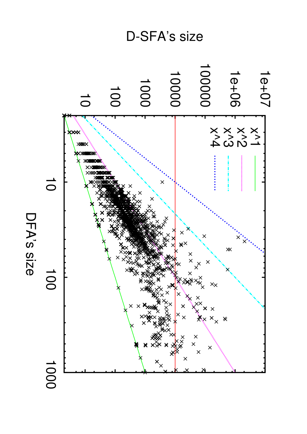
We would like to discuss the number of states in D-SFA from two viewpoints: absolute size of D-SFA and relative size of D-SFA compared with DFA. Firstly, only 102 (0.5%) regular expressions lead to D-SFA that have more than 10000 states. As we discuss later, current CPUs efficiently compute automata with 10000 states. Therefore, for almost all the practical regular expressions, we can use D-SFA for efficient parallel matching.

Secondly, for almost all the regular expressions, the number of states in the D-SFA is not more than the square of the number of states in the minimal DFA. Only 279 (1.4%) regular expressions lead to a D-SFA of over-square size ( $|{\cal S}_{d}|>|D|^{2}$ ), and just 6 regular expressions lead to a D-SFA of over-cubed size ( $|{\cal S}_{d}|>|D|^{3}$ ). These 6 regular expressions have a pattern similar to:

\mathtt{.*(T.*T.*Y.*P.*P.*R.*O.*M.*P.*T.*)}

in which several .* appear in sequence. For the above regular expression, the size of the minimal DFA is 10 but the size of D-SFA is 3739. It is worth noting that no regular expressions in the rulesets lead to a D-SFA of over-quadruplicate size ( $|{\cal S}_{d}|>|D|^{4}$ ).

In theory, the size of a D-SFA $|{\cal S}_{d}|$ is bounded by $|{\cal D}|^{|{\cal D}|}$ where $|{\cal D}|$ is the size of the DFA from which the D-SFA is constructed (Table II). From the experiment results, however, we conclude that the size of D-SFA never grows up exponentially for practical regular expressions. Of course, in a theoretical perspective, there exist regular expressions that lead to N-SFA or D-SFA of near upper-bound sizes. We will discuss them in Sect. VII-B.

VI-B Scalability

Second question is “Does the SFA-based parallel matching scale?” We confirmed the scalability of the parallel computation of SFA with regular expressions in the following form:

r_{n}=\mathtt{([0-4]\{}n\mathtt{\}[5-9]\{}n\mathtt{\})*}

for $n=5$ , $50$ , and $500$ . It is worth noting that the sizes of D-SFA for these expressions are almost the square of those of DFA. For better understanding, we illustrate the minimal DFA in Fig. 4 and the corresponding D-SFA in Fig. 5 for the case $n=2$ . The DFA has $2n$ states in a single loop, but the D-SFA has $2n$ loops to distinguish from which state (in DFA) we start. This is a typical case when we have square-sized D-SFA.

Figures 9 to 9 show the throughput of the DFA or D-SFA. Note that the results with one thread were of DFA (and not D-SFA). The input texts were 1GB string accepted by those automata, and every character was read exactly once. The input texts were stored on the memory before the execution.

As seen in Figures 9 and 9, the SFA-based parallel matching scales well up to 12 threads (with respect to the sequential DFA-base matching). However, in Fig. 9, the SFA-based parallel matching ran slower (even with 12 threads) than sequential DFA-based matching. The difference between them was the size of SFA (and DFA). For $r=50$ , the number of states in SFA was 10099 and parallel matching performed well for this size. For $r=500$ , the number of states in SFA was 1000999 while the number of states in DFA was 1000. In our implementation, the transition table occupied 1KB for each state (256 symbols times 4 bytes). For $r=500$ the transition table for SFA was 1GB and thus it overflowed the CPU cache (The L3 cache of the CPU was 12MB).

It is worth noting that the large size of SFA does not always mean the poor performance. It is often the case that transitions are done among small number of states, and then we can avoid cache misses fortunately. Figure 9 shows the experiment results for the regular expression ([0-4]{500}[5-9]{500})*|a* and input text being a repetition of “a”. Although the number of states in SFA was the biggest (1001000), it achieved the best throughput. In this case, the transitions were done in a single state and cache misses were avoided.

VI-C Overheads

We conducted another set of experiments using a smaller input to evaluate the overhead. Figure 10 shows the execution times of the sequential computation of DFA and the parallel computation of SFA with two threads. The execution times of the parallel computation includes the creation of threads and the reduction. Here we used regular expression (([02468][13579]){5})* (the size of DFA is 10, and the size of SFA is 21). Though the execution time of the parallel computation swings caused by interfere between threads, but the parallel computation runs faster in average over 600KB, and completely over 800KB.

Finally we briefly remark on the cost of constructing SFA. Table III shows the time required to constructing DFA and SFA for the regular expressions $r_{n}=\mathtt{([0-4]\{}n\mathtt{\}[5-9]\{}n\mathtt{\})*}$ . Though the correspondence construction of D-SFA from DFA is slower than construction of DFA because we need to calculate the mapping between states, it is fast enough to generate about 50000 states per second. As we have seen in Fig. 3, D-SFA for almost all the practical regular expressions are smaller than 10000 states, and thus we can construct them in less than 0.2 seconds.

TABLE III: Times (in sec) for constructing DFA and D-SFA for

r_{n}=\mathtt{([0-4]\{}n\mathtt{\}[5-9]\{}n\mathtt{\})*}

	$r_{5}$	$r_{50}$	$r_{500}$
DFA ${\cal D}$	0.0003	0.0019	0.0187
$\|{\cal D}\|$	10	100	1000
D-SFA ${\cal S}_{d}$	0.0020	0.2020	23.937
$\|{\cal S}_{d}\|$	109	10099	1000999

VII Discussion

VII-A Syntactic monoid

In this paper, we proposed simultaneous finite automaton (SFA) as a data-parallel model of regular expression matching. SFA are natural extensions of finite automata on the automata theory. In addition, SFA can be regarded as special cases of DFA that include the structure of a syntactic monoid [19, 13], which is an algebraic characterization of the regular language. We would like to emphasize that SFA will bridge the gap between the practice of automata and abstract theory of syntactic monoid.

The size of a syntactic monoid for a regular language is called syntactic complexity. Indeed, syntactic complexity of a regular language is also the size of a minimal SFA of the identical language. So far, syntactic complexity has received less attention than state complexity that is the size of a minimal DFA [20].

As we have shown in this paper, SFA provide a data-parallel model of regular expression matching, and thus we can say that syntactic complexity is also parallel complexity of regular expressions. We expect that syntactic complexity gets more attentions for establishing the theory over automata and their parallelization.

VII-B The state explosion problem: an algebraic approach

Here we discuss the theoretical upper bound of the number of states in SFA. First, we see an example in which we construct a DFA from an NFA followed by a D-SFA from the DFA.

Example 3

Consider $\Sigma=\{\mathtt{a,l,p}\}$ and the regular expression $e=\mathtt{[ap]*[al][alp]\{}n-2\mathtt{\}}$ . Figure 11 shows the NFA ${\cal N}_{ex\ref{ex:upper_dfa}}$ of the regular expression $e$ .

Let us represent the set of states in NFA by a bit-sequence of length $n$ . Then, the initial set of states in Fig. 11 is $1\underbrace{00\cdots 0}_{n-1}$ . The symbols $\mathtt{a}$ and $\mathtt{l}$ make the following transitions from the initial set of states:

	$\displaystyle 1\underbrace{00\ldots 0}_{n-1}$	$\displaystyle\xrightarrow{\mathtt{a}}$	$\displaystyle 11\underbrace{00\ldots 0}_{n-2}~\hbox{, and}$
	$\displaystyle 1\underbrace{00\ldots 0}_{n-1}$	$\displaystyle\xrightarrow{\mathtt{l}}$	$\displaystyle 01\underbrace{00\ldots 0}_{n-2}~,$

and the symbol $\mathtt{p}$ makes the following transitions:

	$\displaystyle 11\underbrace{00\ldots 0}_{n-2}$	$\displaystyle\xrightarrow{\mathtt{p}}$	$\displaystyle 101\underbrace{00\ldots 0}_{n-3}~\hbox{, and}$
	$\displaystyle 01\underbrace{00\ldots 0}_{n-2}$	$\displaystyle\xrightarrow{\mathtt{p}}$	$\displaystyle 001\underbrace{00\ldots 0}_{n-3}~.$

Notice that the symbols $\mathtt{a}$ and $\mathtt{l}$ correspond to arithmetic shift and logical shift and the symbol $\mathtt{p}$ corresponds to partial shift applied to bit-sequences from second bit. With these three shift operations, we can generate all the bit-sequences of length $n$ from the initial sequence. Hence the minimal DFA ${\cal D}_{ex\ref{ex:upper_dfa}}$ of ${\cal N}_{ex\ref{ex:upper_dfa}}$ satisfies $|{\cal D}_{ex\ref{ex:upper_dfa}}|=2^{|{\cal N}_{ex\ref{ex:upper_dfa}}|}$ . $\diamond$

By Example 3, we obtain the following fact.

Fact 1

If $|\Sigma|\geq 3$ , then there exists a regular expression $e$ over $\Sigma$ whose NFA ${\cal N}$ and minimal DFA ${\cal N}$ satisfies $|{\cal D}|=2^{|{\cal N}|}$ . $\diamond$

Based on a similar idea, we can find a regular expression for which a D-SFA has as many states as the theoretical upper bound from the size of DFA.

Example 4

Consider $\Sigma=\{\mathtt{c,m,t}\}$ and the regular expression $e=\mathtt{(m|(t|c([mt]*c)\{}n-2\mathtt{\})[cmt])*}$ . Figure 12 shows the minimal DFA ${\cal D}_{ex\ref{ex:upper_dsfa}}$ of the regular expression $e$ . The minimal D-SFA ${\cal D}_{ex\ref{ex:upper_dsfa}}$ of ${\cal S}_{ex\ref{ex:upper_dsfa}}$ satisfies $|{\cal S}_{ex\ref{ex:upper_dsfa}}|=|{\cal D}_{ex\ref{ex:upper_dsfa}}|^{|{\cal D}_{ex\ref{ex:upper_dsfa}}|}$ . $\diamond$

By Example 4, we obtain the following fact.

Fact 2

If $|\Sigma|\geq 3$ , then there exists a regular expression $e$ over $\Sigma$ whose minimal DFA ${\cal D}$ and minimal D-SFA ${\cal S}_{d}$ satisfies $|{\cal S}_{d}|=|{\cal D}|^{|{\cal D}|}$ . $\diamond$

Facts 1 and 2 mean the existence of regular expressions with three symbols that lead to state explosion in the construction of DFA or D-SFA. Here, we have another question: Is there a regular expression with a constant number of symbols that lead to state explosion in the construction of N-SFA from NFA? The following fact on the semigroup theory gives a negative answer to this question.

Fact 3 (Devadze [21, 22])

The size of a minimal generating set of the semigroup of $n\times n$ boolean matrices grows exponentially with $n$ . $\diamond$

This fact was first presented by Devadze in 1968, and he described minimal sets of generators of the semigroup of $n\times n$ boolean matrices without a proof. Its was proved very recently by Konieczny in 2011 [22].

We stated in the previous section that the states in SFA correspond to elements in syntactic monoid. Since the syntactic monoid can be represented with boolean matrices and their multiplication ²² 2 See [23, 19] for the relation between the syntactic monoid and boolean matrices. Theorem 3 in [23] is a proof for Fact 2. In the semigroup theory, the problem corresponding to Fact 2 is one of basic propositions ([24], Exercise 6)., the theorem also applies to the syntactic monoid.

The following fact follows from Devadze’s theory.

Corollary 3.1

To denote a regular expression that leads to an N-SFA ${\cal S}_{n}$ with $|{\cal S}_{n}|=2^{k^{2}}$ states, we require an exponential number of states with respect to $k$ . $\diamond$

Corollary 3.1 means that it is unrealistic to find a large regular expression that leads to state explosion in the construction of N-SFA.

VIII Conclusion

We have defined a novel class of automata called simultaneous finite automata, and developed an implementation of them for efficient data-parallel regular expression matching. The parallel computation of SFA runs in $\mathrm{O}(n/p+p)$ time or in $\mathrm{O}(n/p+|{\cal D}|\log p)$ time where $|{\cal D}|$ is the number of states in DFA, $n$ is the length of input word and $p$ is the number of threads.

We tackled SFA’s size issue in Sect. VI-A, made experiments in real world regular expressions (SNORT rulesets), and show that SFA’s size is fully practical in typical case. We also made experiments with the SFA-based regular expression matcher, and confirmed good scalability by a factor of over 10 on an environments with dual hexa-core CPUs and small overhead such that execution with two threads outperforms for input data over 600KB.

Our implementation of the SFA-based parallel regular expression matcher is available as an open-source software [9], hence anyone can verify the experimental results in Sect. VI.

Acknowledgments

We would like to thank Kazuhiro Inaba for the helpful discussion with him on the prior works described in Sect. III and Sect. VII-B.

This work was partly supported by the joint project between ANR (France) and JST (Japan) (project PaPDAS ANR-2010-INTB-0205-02 and JST 10102704).

References

[1] S. Kumar, S. Dharmapurikar, F. Yu, P. Crowley, and J. Turner, “Algorithms to accelerate multiple regular expressions matching for deep packet inspection,” SIGCOMM Comput. Commun. Rev., vol. 36, no. 4, pp. 339–350, Aug. 2006. [Online]. Available: http://doi.acm.org/10.1145/1151659.1159952
[2] B. C. Brodie, D. E. Taylor, and R. K. Cytron, “A scalable architecture for high-throughput regular-expression pattern matching,” SIGARCH Comput. Archit. News, vol. 34, no. 2, pp. 191–202, May 2006. [Online]. Available: http://doi.acm.org/10.1145/1150019.1136500
[3] R. E. Ladner and M. J. Fischer, “Parallel prefix computation,” Journal of the ACM, vol. 27, no. 4, pp. 831–838, 1980.
[4] W. D. Hillis and G. L. Steele, Jr., “Data parallel algorithms,” Commun. ACM, vol. 29, no. 12, pp. 1170–1183, Dec. 1986. [Online]. Available: http://doi.acm.org/10.1145/7902.7903
[5] J. Holub and S. Štekr, “On parallel implementations of deterministic finite automata,” in Implementation and Application of Automata, 14th International Conference, CIAA 2009, Proceedings, ser. Lecture Notes in Computer Science, vol. 5642. Springer, 2009, pp. 54–64.
[6] D. Luchaup, R. Smith, C. Estan, and S. Jha, “Multi-byte regular expression matching with speculation,” in Proceedings of the 12th International Symposium on Recent Advances in Intrusion Detection, ser. RAID ’09. Berlin, Heidelberg: Springer-Verlag, 2009, pp. 284–303. [Online]. Available: http://dx.doi.org/10.1007/978-3-642-04342-0_15
[7] ——, “Speculative parallel pattern matching,” Trans. Info. For. Sec., vol. 6, no. 2, pp. 438–451, Jun. 2011. [Online]. Available: http://dx.doi.org/10.1109/TIFS.2011.2112647
[8] Y. Ko, M. Jung, Y.-S. Han, and B. Burgstaller, “A speculative parallel DFA membership test for multicore, SIMD and cloud computing environments,” CoRR, vol. abs/1210.5093, 2012.
[9] R. Sin’ya, “Regen: regular expression generator, engine, JIT-compiler.” [Online]. Available: http://sinya8282.github.com/Regen/
[10] P. D. Stotts and W. Pugh, “Parallel finite automata for modeling concurrent software systems,” Journal of Systems and Software, vol. 27, pp. 27–43, 1994.
[11] M. Jantzen, M. Kudlek, and G. Zetzsche, “Concurrent finite automata,” in Tagungsband 17. Theorietag Automaten und Formale Sprachen, M. Droste and M. Lohrey, Eds., 2007, pp. 84–88.
[12] A. K. Chandra, D. C. Kozen, and L. J. Stockmeyer, “Alternation,” J. ACM, vol. 28, no. 1, pp. 114–133, Jan. 1981. [Online]. Available: http://doi.acm.org/10.1145/322234.322243
[13] J. Sakarovitch, Elements of Automata Theory. Cambridge University Press, 2009.
[14] M. O. Rabin and D. Scott, “Finite automata and their decision problems,” IBM Journal of Research and Development, vol. 3, no. 2, pp. 114–125, 1959.
[15] R. Cox, “Regular expression matching can be simple and fast,” 2009. [Online]. Available: http://swtch.com/~rsc/regexp/regexp1.html
[16] A. V. Aho, R. Sethi, and J. D. Ullman, Compilers: Principles, Techniques, and Tools, second edition ed. Prentice Hall, 2006.
[17] R. McNaughton and H. Yamada, “Regular expressions and state graphs for automata,” IRE Transactions on Electronic Computers, vol. EC-9, no. 1, pp. 39–47, 1960.
[18] M. Roesch, “Snort: Lightweight intrusion detection for networks,” in Proceedings of the 13th Conference on Systems Administration (LISA-99). USENIX, 1999, pp. 229--238.
[19] J.-E. Ṕin, Syntactic Semigroups. Springer-Verlag, 1997, vol. 1, ch. 10, pp. 679–746, g. Rozenberg and A. Salomaa (eds). Handbook of Formal Languages.
[20] J. A. Brzozowski, B. Li, and Y. Ye, “Syntactic complexity of prefix-, suffix-, and bifix-free regular languages,” in Descriptional Complexity of Formal Systems — 13th International Workshop, DCFS 2011, Proceedings, ser. Lecture Notes in Computer Science, vol. 6808, 2011, pp. 93–106.
[21] H. M. Devadze, “Generating sets of the semigroup of all binary relations on a finite set.” 1968, pp. 765–768, russian.
[22] J. Konieczny, “A proof of Devadze’s theorem on generators of the semigroup of boolean matrices.” Semigroup Forum, vol. 83, no. 2, pp. 281–288, 2011.
[23] M. Holzer and B. König, “On deterministic finite automata and syntactic monoid size,” Theoretical Computer Science, vol. 327, no. 3, pp. 319–347, 2004.
[24] J. M. Howie, Fundamentals of Semigroup Theory (London Mathematical Society Monographs New Series). Oxford University Press, USA, Feb. 1996.

Model	State complexity	Computation time complexity
NFA ${\cal N}$	$\|{\cal N}\|=\mathrm{O}(m)$	$\mathrm{O}(\|{\cal N}\|n)$ ([16] p.165)
DFA ${\cal D}$	$\|{\cal D}\|=\mathrm{O}(2^{\|{\cal N}\|})$	$\mathrm{O}(n)$ (Algorithm 2)
		$\mathrm{O}(\|{\cal D}\|n/p+\|{\cal D}\|\log p)$ (Algorithm 3)
		$\mathrm{O}(\|{\cal D}\|n/p+p)$ (sequential reduction)
N-SFA ${\cal S}_{n}$	$\|{\cal S}_{n}\|=\mathrm{O}(2^{\|{\cal N}\|^{2}})$	$\mathrm{O}(n/p+\|{\cal N}\|^{3}\log{p})$
		$\mathrm{O}(n/p+\|{\cal N}\|p)$ (sequential reduction)
D-SFA ${\cal S}_{d}$	$\|{\cal S}_{d}\|=\mathrm{O}(\|{\cal D}\|^{\|{\cal D}\|})$	$\mathrm{O}(n/p+\|{\cal D}\|\log{p})$
		$\mathrm{O}(n/p+p)$ (sequential reduction)

Simultaneous Finite Automata: An Efficient Data-Parallel Model for Regular Expression Matching

Abstract

I Introduction

II Preliminaries

II-A Notation

II-B Finite Automata

Definition 1

Definition 2

Definition 3

Definition 4

Theorem 1 (Rabin and Scott[14])

Proof:

II-C Subset Construction and Sequential Computation in DFA

III Prior Works: Parallel Computation in DFA with Speculative Simulation

IV Simultaneous Finite Automata

IV-A Formal Definition

Definition 5

Theorem 2

Proof:

IV-B Example

Example 1

IV-C Data-Parallel Property of SFA

Lemma 1

Proof:

Theorem 3

Proof:

V Implementing SFA

V-A Construction of SFA from Finite Automaton

V-B Parallel Computation in SFA

Example 2

VI Experimental Results

VI-A The size of SFA

VI-B Scalability

VI-C Overheads

VII Discussion

VII-A Syntactic monoid

VII-B The state explosion problem: an algebraic approach

Example 3

Fact 1

Example 4

Fact 2

Fact 3 (Devadze [21, 22])

Corollary 3.1

VIII Conclusion

Acknowledgments

References

Simultaneous Finite Automata:
An Efficient Data-Parallel Model
for Regular Expression Matching