A Parallel Orbital-Updating Approach for Electronic Structure Calculations Thanks: This work was partially supported by the Funds for Creative Research Groups of China under grant 11321061, the National Basic Research Program of China under grant 2011CB309703, the National Science Foundation of China under grants 11101416 and 91330202, the National 863 Project of China under grant 2012AA01A309, and the National Center for Mathematics and Interdisciplinary Sciences of Chinese Academy of Sciences.

To handle the Coulomb potential or the highly oscillating behaviors of eigenfunctions efficiently, we apply an adaptive finite element approach to discretize the associated source problems. An adaptive finite element algorithm usually consists of the following loop [7, 8, 10, 12]:

We shall replace the subscript $h$ (or $h_{k}$) by an iteration counter $k$ whenever convenient afterwards.

Solve. Get the piecewise polynomial finite element approximation with respect to a given mesh $\mathcal{T}_{k}$.

Estimate. Given a mesh $\mathcal{T}_{k}$ and the corresponding output from the “Solve” step, “Estimate” presents the a posteriori error estimators $\{\eta_{k}(\cdot,\tau)\}_{\tau\in\mathcal{T}_{k}}$.

Mark. Based on the a posteriori error indicators $\{\eta_{k}(\cdot,\tau)\}_{\tau\in\mathcal{T}_{k}}$, “Mark” provides a strategy to choose a subset $\mathcal{M}_{k}$ of elements of $\mathcal{T}_{k}$ for refining.

Refine. Associated with the mesh $\mathcal{T}_{k}$ and the set of marked elements $\mathcal{M}_{k}$, “Refine” produces a new mesh $\mathcal{T}_{k+1}$ by refining all elements in $\mathcal{M}_{k}$ at least one time.

One of the most widely used marking strategy to enforce error reduction is the following so-called Dörfler strategy [14].

Dörfler Strategy. Given a marking parameter $0<\theta<1$ :

1. 1.

   Choose a subset $\mathcal{M}_{k}\subset\mathcal{T}_{k}$ such that

   (2.2)

   $\displaystyle\sum_{\tau\in\mathcal{M}_{k}}\eta^{2}_{k}(\cdot,\tau)\geq\theta\sum_{\tau\in\mathcal{T}_{k}}\eta^{2}_{k}(\cdot,\tau).$

2. 2.

   Mark all the elements in $\mathcal{M}_{k}$.

The “Maximum Strategy” is another wildly used marking strategy.

Maximum Strategy. Given a marking parameter $0<\theta<1$ :

1. 1.

   Choose a subset $\mathcal{M}_{k}\subset\mathcal{T}_{k}$ such that

   (2.3)

   $\displaystyle\eta_{k}(\cdot,\tau)\geq\theta\max_{\tau\in\mathcal{T}_{k}}\eta_{k}(\cdot,\tau).$

2. 2.

   Mark all the elements in $\mathcal{M}_{k}$.

In our computation, we apply the shape-regular bisection for the refinement. We refer to [8, 10] for more details for the adaptive finite element computations for Kohn-Sham DFT.

The Kohn-Sham equation of a molecular system consisting of $M$ nuclei of charges $\{Z_{1},\cdots,Z_{M}\}$ located at positions $\{{\bf R}_{1},\cdots,{\bf R}_{M}\}$ and $N_{e}$ electrons in the non-relativistic and spin-unpolarized setting is the following nonlinear eigenvalue problem

where $\displaystyle\rho(x)=\sum_{i=1}^{N}|u_{i}(x)|^{2}$ is the electron density, $V_{H}(\rho)=\frac{1}{2}\int_{\mathbb{R}^{3}}\frac{\rho(y)}{|x-y|}dy$ denotes the Hartree potential, $V_{\rm xc}(\rho)$ indicates the exchange-correlation potential, and $\displaystyle V_{\rm ext}(x)$ is the electrostatic potential generated by the nuclei, including both full-potentials and pseudopotential approximations. For full-potentials, $N=N_{e}$ and $\displaystyle V_{\rm ext}(x)=-\sum_{k=1}^{M}\frac{Z_{k}}{|x-{\bf R}_{k}|}$. While for pseudopotential approximations, $N$ equals to the number of valence electrons, $V_{\rm ext}=V_{\rm loc}+V_{\rm nl}$, with $V_{\rm loc}$ being the local part of pseudopotential and $V_{\rm nl}$ being a nonlocal part given by (see, e.g., [23])

with $n\in\mathbb{N}$ and $\zeta_{j}\in L^{2}(\Omega)(j=1,2,\cdots,n)$.

By density functional theory (DFT) [17, 19](see, also, [23, 25]), the ground state (charge) density of the system may be obtained by solving the lowest $N$ eigenpairs of (2.2). In computation, $V_{H}(\rho)$ is usually obtained by solving the following Poisson equation:

The exact formula for exchange-correlation potential $V_{xc}$ is unknown. Some approximation (such as LDA, GGA) has to be used.

Note that the ground state wavefunction of the Schrödinger equation and the solutions of Kohn-Sham model are exponentially decay [2, 3, 30], $\mathbb{R}^{3}$ is then replaced by some polyhedral domain $\Omega\subset\mathbb{R}^{3}$ in computation. Instead of (2.2), more precisely, we solve

where $U=(u_{1},u_{2},\cdots,u_{N})$ and $a(U;\cdot,\cdot):H_{0}^{1}(\Omega)\times H_{0}^{1}(\Omega)\rightarrow\mathbb{R}$ is defined by

with $\rho_{{}_{U}}=\displaystyle\sum^{N}_{i=1}|u_{i}|^{2}.$

Consider a finite dimensional discretization of (2.2) as follows:

where $V_{n}$ is some finite dimensional space. We see that (3.1) is a nonlinear eigenvalue problem, and the so called self-consistent field (SCF)(see, e.g., [20, 24]) iteration approaches are often used to linearize it.

We may divide the finite dimensional discretizations for Kohn-Sham equations into three classes: the plane wave method, the local basis set method, and the real space method. The plane wave method uses plane wave functions as the basis functions to span a finite dimensional space $V_{n}$, while the local basis set method uses some Slater type or Gaussian type functions as the bases to construct a finite dimensional space $V_{n}$. The finite element method is one of commonly used real space methods, where finite element bases are used to construct $V_{n}$. No matter what kind of methods are used to discretize the Kohn-Sham equation, after linearization, what we get is some algebraic eigenvalue problem $Au=\lambda Bu$, where $A$ is the stiff matrix, $B$ is the mass matrix. And we need to solve the first $N$ eigenvalues and the corresponding eigenfunctions of the algebraic eigenvalue problem. If $A$ and $B$ are sparse, e.g., discretized by a finite element method, then the optimal computational complexity is $\mathcal{O}(N^{2}N_{g})$, while if $A$ or $B$ is dense, e.g., discretized by a plane wave method or a local basis set method, then the optimal computational complexity becomes $\mathcal{O}(NN_{g}^{2})$. Here, $N_{g}$ is the dimension of the matrix. We see that $N_{g}\gg N$ or a practically complete basis set is difficult to obtain. Note that to obtain an accurate approximation, one needs to solve tens of such algebraic eigenvalue problems, which limits the application of Kohn-Sham DFT to large scale systems, especially for full-potential calculations.

We have already seen that the huge computational complexity for solving the discretized eigenvalue problems limits the application of Kohn-Sham DFT to the electronic structure calculations for large scale systems. Hence, a faster, accurate and efficient algorithm for solving Kohn-Sham equations as well as other eigenvalue problems is desired. In this subsection, we propose some new approach that can reduce the computational complexity remarkably, as compared with the existing methods of solving Kohn-Sham equations.

We understand that the Kohn-Sham equation is established within the framework of single-particle approximation, and can be viewed as a set of single-particle equations of independent particles that move in an effective potential. Motivated by the setting that independent particle moves in an efficient potential, we are indeed able to carry out these single-particle orbitals individually or in parallel intrinsically. It is shown by our investigation that a simple iteration with some observational data would be efficient for a special situation and supercomputers.

We note that for solving a large scale eigenvalue problem, an iteration scheme is usually used, which can also be view as ( a discretized version of) some motion. Based on our understanding that the basic rule of motion is simple but the initial data may be special, we propose the following parallel orbital-updating algorithm for solving the Kohn-Sham equation based on finite element discretizations.

In our computation in Section 4, we choose $V_{n}$ as some finite element space $S_{0}^{h_{n},k}(\Omega)$ over $\mathcal{T}_{n}$ with some $k$, the degree of piecewise polynomials. While $\mathcal{T}_{n}$ is constructed based on some a posteriori error estimations of $(\lambda^{(n)}_{i},u_{i}^{(n)})$, marking strategy and refine procedure as described in Section 2.1. Indeed, $V_{n}$ can also be any other appropriate relevant finite dimensional spaces.

We see that to provide a physical observational data is natural and significant for algorithm’s efficiency. In electronic structure calculations, we may choose the initial data $(\lambda^{(0)}_{i},u_{i}^{(0)})$ as follows:

• •

  Gaussian-type orbital or Slater-type orbital based guesses, which are applicable to full-potential calculations,

• •

  local plane-wave discretization based guesses, which are applicable to pseudo-potential settings,

• •

  local finite element/volume discretization based guesses (c.f., e.g.,[9, 10, 11, 13]), which are applicable to either full-potential calculations or pseudo-potential settings.

It will be demonstrated by our experiments in Section 4 that the parallel orbital-updating approach is powerful in electronic structure calculations. Here we mention several features of Algorithm 3.1 as follows:

• •

  Model linearization. We understand from Algorithm 3.1 that our parallel orbital-updating approach is in fact some new SCF iteration technique and mixes simple discretization iterations of source problems with adaptive computations.

• •

  Complexity reduction. We see form our new algorithm that the solution of the original tens of large scale eigenvalue problems is reduced to the solution of some independent source problems and some small scale eigenvalue problems. Since these source problems are independent each other, our parallel orbital-updating algorithm can be carried out in parallel intrinsically. Indeed, the computational complexity then becomes $\mathcal{O}(N_{g}+N_{orb}^{3})$, which is much lower than $\mathcal{O}(N_{orb}^{2}N_{g})$ or $\mathcal{O}(N_{orb}N_{g}^{2})$, the costs for solving the Kohn-Sham equation directly, where $N_{orb}$ is the number of desired eigenvalues and $N_{g}$ is the number of unknowns of the discretized Kohn-Sham equation or the dimension of the resulting matrix.

• •

  Eigenvalue separation. If the initial guess is well-posed, then we are able to obtain the orbital approximations individually. For illustration, we comment the more general setting Algorithm A.1 rather than Algorithm 3.1, which is applied to solve eigenvalue problem (A.3).

  For $\lambda\in\sigma(L)$, define

  $$\delta(\lambda)=\inf\{\|w-v\|_{l,\Omega}:w\in M(\lambda),v\in M(\mu),\mu\in\sigma(L)\setminus\{\lambda\}\}.$$

  Let $\mu_{i}\in\sigma(L)$ whose multiplicity is $q_{i}(i=1,2,\cdots,M)$, respectively¹¹ 1 In our discussion, $q_{1}=1$ when $\mu_{1}=\lambda_{1}$.. Assume that the initial data $(\lambda^{(0)}_{i+j},u_{i+j}^{(0)})\in\mathbb{R}\times H^{1}_{0}(\Omega)$ satisfying that $\|u^{(0)}_{i+j}\|_{0,\Omega}=1(i=1,2,\cdots,M;j=0,1,2,\cdots,q_{i}-1)$ and $\mbox{span}\{u_{i+j}^{(0)}:j=0,1,2,\cdots,q_{i}-1\}$ away from

  $$\cup\left\{M(\mu):\mu\in\sigma(L)\setminus\{\mu_{i}\}\right\},~i=1,2,\cdots,M.$$

  More precisely, for $i=1,2,\cdots,M$,

  $$\inf\{\|u^{(0)}_{i+j}-v\|_{0,\Omega}:j=0,1,2,\cdots,q_{i}-1;v\in M(\mu),\mu\in\sigma(L)\setminus\{\mu_{i}\}\}>\delta(\mu_{i})/2.$$

  Then we may apply Algorithm A.1 to obtain eigenspace approximations in parallel. We observe that the computational cost

  $$\mathcal{O}\left(\left(\sum_{i=1}^{M}q_{i}\right)^{3}\right)$$

  of computing eigenpairs is then reduced to

  $$\mathcal{O}\left(\sum_{i=1}^{M}q_{i}^{3}\right).$$

• •

  Two-level parallelization. We may also see a potential of our algorithm in large scale parallel computation. Since these source problems are independent each other, they can be calculated in parallel intrinsically, and each source problems can also be solved in parallel by various multigrid or domain decomposition approaches, which is a two level parallelization. One level is the solution of these $N$ independent source problems in parallel intrinsically, another level is to solve each source problem in parallel by using idea of multigrid or domain decomposition methods. As a result, there may be some potential for E-scale eigenvalue computations.

We point out that if the initial guess is not well-provided, then we suggest to apply the following algorithm:

It tells from Algorithm 3.2 that more eigenpairs should be computed so as to get a better approximation of the first $N$ orbitals. In practice, we see that Algorithm 3.2 is more stable than Algorithm 3.1.

We may refer to Appendix for a generalization to a class of linear eigenvalue problems and its basic numerical analysis.

First, we will validate the reliability of our algorithm by using a small molecular system as example. As well known, for small atomic or molecular systems, Gaussian09 provides very efficient and accurate results To illustrate the reliability of our algorithm, we use $H_{2}O$ as an example to show that the results obtained by our algorithm are reliable by comparing with those obtained by Gaussian09.

Example 1: $H_{2}O$

The atomic configuration for molecule $H_{2}O$ is figured in Fig. 1. Here we compute the first $5$ eigenpairs of the associated Kohn-Sham equation.

Table 1 provides the detailed information for results obtained by Gaussian09 with different kinds of basis functions being used and those obtained by our algorithm after different number of iterations. The second column is the total energy obtained, the third column is the number of basis functions used, the forth column is the wall-time cost, while the fifth column is the number of processors used.

It should be pointed out that in our current numerical experiments, the $N_{orb}$ number of boundary value problems are solved one by one, not in parallel, and here the multi processors deal with only the parallelization in space, not in orbital. That is, the $N_{orb}$ boundary value problems $(\ref{alg-bvp})$ are solved one by one, not in parallel. If we have enough processors, the $N_{orb}$ boundary value problems can be carried out in parallel intrinsically, the wall-time cost by our algorithm would be reduced further, and it is listed in the last column with color red.

We observe from Table 1 that for Gaussian09, as the bases changes from STO-3G to cc-pV6Z, the total ground state energy approximation reduces from large to small, while the corresponding cpu-time cost increases fastly, especially when the ground state energy approximation is closed to the exact one. For example, when using bases from cc-pV5Z to cc-pV6Z, the total energy decreases about $0.00081$ a.u., while the cpu-time cost increases 1088s. More precisely, for the basis set method, the cost is not expensive if only less accurate result is required, while the cost will become very huge if the the accuracy of approximation increases a little bit after some critical accuracy.

We see that the ground state energy approximations obtained by our algorithm after $116$ iterations( here, $1$ iteration means doing Step 2, Step 3, and Step 4 of Algorithm 3.1 once) is $-75.908257$ a.u., which is very close to that obtained by Gaussian09 using basis cc-pV5Z, and if we refine the mesh adaptively and do one iteration again , then the ground state energy approximation will decrease further. Let us take a more detailed. After $149$ iterations, the energy approximation decreases to $-75.909026$ a.u., close to the results obtained by Gaussian09 using basis cc-pV6Z. If we do more iterations, that is, after $166$ iterations, the energy approximation decreases to $-75.909175$ a.u., smaller than that obtained by Gaussian09 using basis cc-pV6Z by $0.000151$ a.u..

Although the total cpu time cost by our algorithm is much longer than that cost by Gaussian09, we should note that the cpu-time cost does not increase as quickly as that for Gaussian09. In fact, for Gaussian09, when the bases are chosen from cc-pV5Z to cc-pV6Z, the total energy approximation decreases from $-75.908214$ a.u. to $-75.909024$ a.u., the cpu-time cost increases from $23$s to $1111$s, about $50$ times of the former one. For our algorithm, from $116$ iterations to $149$ iterations, the energy approximation decreases from $-75.908257$ a.u. to $-75.909026$ a.u., the cpu-time cost increases from $1096.8$s to $2863.6$s, only about $3$ times of the former one.

Fig. 2 shows the convergence curve for the ground state energy approximations over each adaptive refined mesh, where the x-axis is the DOFs, and the y-axis is the ground state energy approximation. We see from Fig. 2 that the total energy approximation converges as the number of degrees increases. For comparison, we show the convergence curve of the total energy obtained by Gaussian09 with different kinds of bases(STO-3G, STO-6G, 6-31G, cc-pVDZ, cc-pVTZ, cc-pVQZ, cc-pV5Z, cc-pV6Z from the right to the left) in Fig. 3.

We may conclude that our algorithm can produce approximations as accurate as or even more accurate than Gaussian09. Although for such a small example, the cpu-time cost by our algorithm is much longer than that cost by Gaussian09, we can see the potential of our algorithm when highly accurate results are desired.

Although Gaussian09 can provide highly accurate results quickly for small molecular systems, it is another story for molecular systems of medium or large size. We see that the memory required for DFT method scales as $N^{4}$ with $N$ being the number of basis functions, for instance.

In this subsection, we will use some molecular systems of medium scale or large scale to show the efficiency of our algorithm.

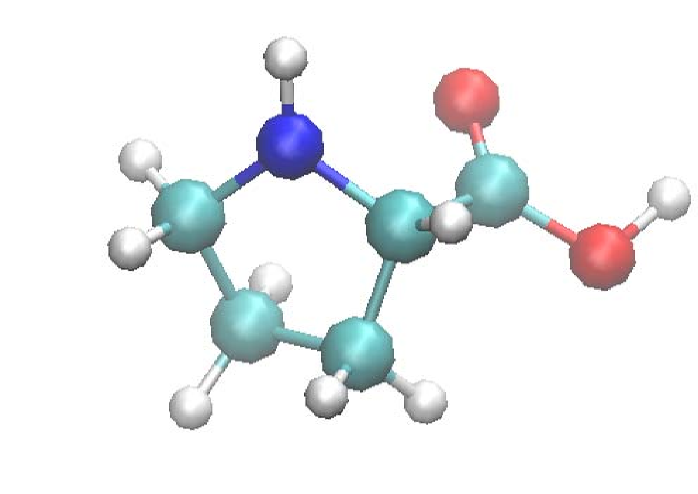
Example 2: $\alpha$-amino acid: $C_{5}H_{9}O_{2}N$

The atomic configuration for molecule $C_{5}H_{9}O_{2}N$ is shown in Fig. 4. For this example, we compute the first $31$ eigenpairs of the Kohn-Sham equation, and $32$ processors are used for both Gaussian09 and our code. Table 2 displays the relevant results.

We see from Table 2 that the total energy approximation obtained by Gaussian09 decreases when the bases are chosen from STO-3G to cc-pV5Z, while the cpu-time cost increases quickly. We mention that due to the huge storage requirement, we are not able to produce the result by Gassian09 using bases cc-pV6Z.

We also observe from Table 2 that after $127$ iterations, the total ground state energy approximations obtained by our algorithm is $-398.009800$a.u., which is close to that obtained by cc-pV5Z. If we refine the mesh adaptively again, we can obtain more accurate results. For example, after $136$ iterations, the total energy approximation decreases to $-398.010611$a.u., which is $0.000729$a.u. smaller than that obtained by Gassian09 using bases cc-pV5Z. The cpu-time cost after $127$ iterations and $136$ iterations are about $19771.6$s and $28868.7$s respectively. As we addressed in Example 1, in our current computations, the $N_{orb}$ number of boundary value problems are solved one by one, not in parallel, and here the $32$ processors deal with only the parallelization in space, not in orbital. Since the $31$ boundary value problems can be carried out in parallel intrinsically, the wall-time cost by our algorithm cost would be at least reduced to $8708.8$s and $12101.5$s respectively provided we have $992(32\times 31)$ processors.

We note from Fig. 5 that the total energy approximation converges as the iteration increases.

Example 3: $C_{9}H_{8}O_{4}$

The atomic configuration for molecule $C_{9}H_{8}O_{4}$ is shown in Fig. 6. We solve the first $47$ eigenpairs of the Kohn-Sham equation.

Table 3 digitizes some relevant results, including those obtained by Gaussian09 and those obtained by our algorithm over the mesh got by $79$ adaptive refinements. Fig. 7 displays the convergence curve of the ground state energy approximation over each adaptive refined mesh.

For this example, the total energy obtained by our algorithm are a little larger than that obtained by Gaussian09 with cc-pV5Z being used.

In this subsection, we apply our algorithm to full-potential electronic structure calculations for some large molecular systems.

Example 4: $C_{17}H_{19}N_{3}$

The configuration for molecule $C_{17}H_{19}N_{3}$ is shown in Fig. 8 and the first $71$ eigenpairs of the Kohn-Sham equation are computed, and $32$ processors are used for both Gaussian09 and our code. Table 4 provides the relevant results.

We observe from Table 4 that after $73$ iterations, the total energy obtained by our algorithm is very close to that obtained by Gaussian09 with using bases cc-pV5Z. Let us take a look at the cpu-time cost. We see that when using the same number of processors, the cpu-time cost by Gaussian09 and our algorithm are $20675.6$s and $33416.7$s, respectively. Note that the $N_{orb}$ boundary value problems are solved one by one, not in parallel. If we apply $2272(=32\times 71)$ processors, indeed, the cpu-time cost by our algorithm can then be reduced to $13885.0$s. If we refine the mesh again, the energy approximation will reduce further. For instance, after $91$ iterations, the total energy approximation will reduce to $-816.493475$, which is $0.026422$ a.u. smaller than that obtained by Gaussian09 with cc-pV5Z being used.

Fig. 9 shows the convergence curve of the ground state energy approximation, from which we conclude that the approximation results obtained by our algorithm converge.

Example 5: $C_{20}H_{14}N_{4}$

The atomic configuration for molecule $C_{20}H_{14}N_{4}$ is shown in Fig. 10 and the first $81$ eigenpairs of the Kohn-Sham equation are approximated.

Table 5 digitizes the computational results, including those obtained by Gaussian09 and those obtained by our algorithm after $58$ and $68$ iterations. Fig. 11 shows the convergence curve of the ground state energy. ¡¡ We get the similar conclusions as that obtained of Example 4 from Table 5 and Fig.11.

Example 6: $C_{60}$

The atomic configuration for molecule $C_{60}$ is shown in Fig. 12 and we compute the first $180$ eigenpairs of the Kohn-Sham equation.

Table 6 digitizes the relevant data. ¡¡ Fig. 13 provides the convergence curves of the total energy after each iteration.

We conclude from Table 6 and Fig. 13 that the similar conclusions as that of Example 4 can be obtained.

¡¡

References

- [1] R.A. Adams, Sobolev Spaces, Academic Press, New York, 1975.
- [2] S. Agmon, Lectures on the Exponential Decay of Solutions of Second-Order Elliptic Operators, Princeton University Press, Princeton, 1981.
- [3] C.O. Almbladh and U. von Barth, Exact results for the charge and spin densities, exchange-correlation potentials, and density-functional eigenvalues, Phys. Rev. B, 31 (1985), pp. 3231-3244.
- [4] O.K. Andersen, Linear methods in band theory, Phys. Rev. B, 12 (1975), pp. 3060-3083.
- [5] P.E. Blöchl, Projector augmented-wave method, Phys. Rev. B, 50 (1994), pp. 17953-17979.
- [6] D.R. Bowler and T. Miyazaki, methods in electronic structure calculations, Report Prog. Pgys., 75 (2012), pp. 036503-03645.
- [7] J.M. Cascon, C. Kreuzer, R.H. Nochetto, and K.G. Siebert, Quasi-optimal convergence rate for an adaptive finite element method, SIAM J. Numer. Anal., 46 (2008), pp. 2524-2550.
- [8] H. Chen, X. Dai, X. Gong, L. He, and A. Zhou, Adaptive finite element approximations for Kohn-Sham models, arXiv:1302.6896, Multi. Model. Simul., to appear.
- [9] H. Chen, L. He, and A. Zhou. Finite element approximations of nonlinear eigenvalue problems in quantum physics, Comput. Meth. Appl. Mech. Engrg., 200 (2011), pp.1846-1865.
- [10] X. Dai, X. Gong, Z. Yang, D. Zhang and A. Zhou, Finite volume discretizations for eigenvalue problems with applications to electronic structure calculations, Mult. Model. Simul., 9(2011), pp.208-240.
- [11] X. Dai, L. Shen, and A. Zhou, , A local computational scheme for higher order finite element eigenvalue approximations, Int. J. Numer. Anal. Model., 5(2008), pp. 570-589.
- [12] X. Dai, J. Xu, and A. Zhou, Convergence and optimal complexity of adaptive finite element eigenvalue computations, Numer. Math., 110 (2008), pp. 313-355.
- [13] X. Dai and A. Zhou, Three-scale finite element discretizations for quantum eigenvalue problems, SIAM J. Numer. Anal., 46 (2008), pp. 295-324.
- [14] W. Dörfler, A convergent adaptive algorithm for Poisson’s equation. SIAM J. Numer. Anal., 33 (1996), pp. 1106-1124.
- [15] E.M. Garau, P. Morin, and C. Zuppa, Convergence of adaptive finite element methods for eigenvalue problems, M3AS, 19 (2009), pp. 721-747.
- [16] Gaussian, http://gaussian.com/.
- [17] P. Hohenberg and W. Kohn, Inhomogeneous electron gas, Phys. Rev. B., 136(1964), pp. 864-871.
- [18] E. Kaxiras, Atomic and Electronic Structure of Solids, Cambridge University Press, Cambridge, UK, 2003.
- [19] W. Kohn and L. J. Sham, Self-consistent equations including exchange and correlation effects, Phys. Rev. A., 140(1965), pp. 4743-4754.
- [20] G. Kresse and J. Furthmüller, Efficient iterative schemes for ab initio total-energy calculations using a plane-wave basis set, Phys. Rev. B., 54(1996), pp. 11169-11186.
- [21] C. Le Bris (ed.), Handbook of Numerical Analysis, Vol. X. Special issue: Computational Chemistry, North-Holland, Amsterdam, 2003.
- [22] S.A. Losilla and D. Sundholm, A divide and conquer real-space approach for all-electron molecular electrostatic potentials and interaction energies, J. Chem. Phys., 136 (2012), pp. 214104-214103.
- [23] R. Martin, Electronic Structure: Basic Theory and Practical Methods, Cambridge university Press, London, 2004.
- [24] M. C. Payne, M. P. Teter, D. C. Allan, T. A. Arias, and J. D. Joannopoulos, Iterative minimization techniques for ab initio total-energy calculations: molecular dynamics and conjugate gradients, Rev. Mod. Phys., 64 (1992), pp.1045-1097.
- [25] R. G. Parr and W. T. Yang, Density-Functional Theory of Atoms and Molecules, Clarendon Press, Oxford, 1994.
- [26] J. P. Perdew and A. Zunger, Self-interaction correction to density-functional approximations for many-electron systems, Phys. Rev. B, 23(1981), pp. 5048-5079.
- [27] PHG,http://lsec.cc.ac.cn/phg/.
- [28] N. Troullier and J.L. Martins, Efficient pseudopotentials for plane-wave calculations, Phys. Rev. B, 43 (1991), pp. 1993-2006.
- [29] D. Vanderilt, Soft slef-consistent pseudopotentials in a generalized eigenvalue formalism, Phys. Rev. B, 41 (1990), pp. 7892-7895.
- [30] H. Yserentant, Regularity and Approximability of Electronic Wave Functions, Lecture Notes in Mathematics, 2000, Springer-Verlag, Berlin, 2010.