An infinite family of prime knots with a certain property for the clasp number

Teruhisa KADOKAMI Kengo KAWAMURA

Abstract

The clasp number $c(K)$ of a knot $K$ is the minimum number of clasp singularities among all clasp disks bounded by $K$ . It is known that the genus $g(K)$ and the unknotting number $u(K)$ are lower bounds of the clasp number, that is, $\max\{g(K),u(K)\}\leq c(K)$ . Then it is natural to ask whether there exists a knot $K$ such that $\max\{g(K),u(K)\}<c(K)$ . In this paper, we prove that there exists an infinite family of prime knots such that the question above is affirmative.

1 Introduction

It is known that every knot in $S^{3}$ bounds a singular disk in $S^{3}$ whose singular set consists of only clasp singularities as illustrated in Figure 1.

Figure 1: A clasp singularity

We call such a singular disk a clasp disk of the knot. Let $K$ be a knot in $S^{3}$ , and $D$ a clasp disk of $K$ . Let $c(D)$ denote the number of clasp singularities in $D$ . Then the clasp number of $K$ is $c(K)=\min\{\,c(D)\,|\,\mbox{$D$ is a clasp disk of $K$}\,\}$ . We refer the reader to [4, 6, 7, 11, 12, 13, 14, 18] for related topics of the clasp number. In this paper, we suppose that every link is in $S^{3}$ and oriented, and the notation of prime knots follows Rolfsen’s book [16].

For a knot $K$ , let $g(K)$ and $u(K)$ be the genus and the unknotting number of $K$ respectively. In [18], T. Shibuya proved that the genus and the unknotting number are lower bounds of the clasp number. In other words, for a knot $K$ we have $\max\{g(K),u(K)\}\leq c(K)$ . Most of the prime knots with up to $10$ crossings satisfy the equality above (cf. Appendix). Then it is natural to ask the following question.

Question 1.1.

Does there exist a prime knot $K$ such that $\max\{g(K),u(K)\}<c(K)$ ?

For an integer $n$ , let $K_{n}$ be the knot as illustrated in Figure 2.

Refer to caption — Figure 2: The knot $K_{n}$

Here, an integer in the rectangle denotes the number of half twists. We note that $K_{0}=\overline{3_{1}}\#4_{1}$ (Figure 4) and $K_{1}=10_{97}$ (Figure 4).

Note that all the knots $K_{n}$ are distinct one another (Proposition 3.1). The main result of this paper is the following theorem. It is the affirmative answer of Question 1.1.

Theorem 1.2.

If $n$ is odd, then the knots $K_{n}$ are prime and we have $\max\{g(K_{n}),u(K_{n})\}<c(K_{n})$ .

In Appendix, we show a table for the clasp numbers of prime knots with up to $10$ crossings. From the table, we raise the following question concerning an upper bound of the clasp number.

Question 1.3.

Let $cr(K)$ be the crossing number of a knot $K$ . For any non-trivial knot $K$ , does the following inequality hold?

c(K)\leq\left[\frac{cr(K)-1}{2}\right],

where $[r]$ denotes the integer part of a rational number $r$ .

Question 1.3 is affirmative for prime knots with up to $10$ crossings (cf. Appendix) and the knots $K_{n}$ (Proposition 3.6). In Section 2, we calculate the Conway polynomial of a knot $K$ with $c(K)\leq 2$ , giving an alternative proof of Morimoto’s result [14] (Lemma 2.1). (Since it seems to be hard to obtain a reference [14], it is also our purpose to expose it to the reader.) Moreover we give a sufficient condition for a knot $K$ to satisfy $c(K)\geq 3$ . In Section 3, we investigate the knots $K_{n}$ and prove Theorem 1.2, and we also prove that Question 1.3 is affirmative for the knots $K_{n}$ .

2 A sufficient condition for a knot $K$ to satisfy $c(K)\geq 3$

In [14], K. Morimoto calculated the Alexander module of a knot from a clasp disk. In this section, we calculate the Conway polynomial of a knot $K$ with $c(K)\leq 2$ , giving an alternative proof of Morimoto’s result [14], and then we give a sufficient condition for a knot $K$ to satisfy $c(K)\geq 3$ .

First, we prove the following lemma.

Lemma 2.1.

(cf. [14]) Let $K$ be a knot with $c(K)\leq 2$ . The Conway polynomial $\nabla_{K}(z)$ of $K$ is expressed as follows:

\begin{array}[]{r}\nabla_{K}(z)=\bigl(b_{1}b_{2}+\varepsilon b_{3}(b_{3}+\delta)\bigr)z^{4}+(b_{1}+b_{2}-\varepsilon\delta)z^{2}+1\\ (b_{1},b_{2},b_{3}\in\mathbb{Z},\ \varepsilon\in\{\pm 1\},\ \delta\in\{0,1\}).\end{array}

Proof..

Let $K$ be a knot with $c(K)\leq 2$ . Then there exists a clasp disk $D$ of $K$ such that $c(D)=2$ . We may assume that $D$ is a surface which is the union of a disk $B_{0}$ and two clasping bands $B_{1}$ and $B_{2}$ (see Figure 5). Here, a clasping band means a pair of embedded $2$ -disks in $S^{3}$ with a clasp singularity as illustrated in Figure 6. The sign of a clasping band is defined as the linking number of the Hopf link bounding the clasping band.

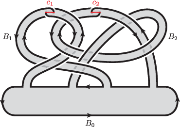
For each $i$ $(i=1,2)$ , let $c_{i}$ be the clasp singularity in $D$ corresponding to the clasping band $B_{i}$ . We define the sign $\varepsilon_{i}\in\{\pm 1\}$ of the clasp singularity $c_{i}$ as the sign of $B_{i}$ . For each $\varepsilon\in\{\pm 1\}$ , an $(\varepsilon)$ -Hopf band is an annulus in $S^{3}$ whose boundary is a Hopf link with linking number $\varepsilon$ . Let $F$ be the oriented surface obtained from $D$ by the following operation:

( $*$ )

For each $i$ $(i=1,2)$ , replacing the neighborhood of the clasp singularity $c_{i}$ with a plumbing of an $(\varepsilon_{i})$ -Hopf band, denoted by $H_{i}$ , as illustrated in Figure 7.

Note that the surface $F$ is a genus two Seifert surface of $K$ . For example, the Seifert surface in Figure 8 is obtained from the clasp disk in Figure 5 by the operation $(*)$ . We take a homological basis $\{[\alpha_{1}],[\alpha_{2}],[\beta_{1}],[\beta_{2}]\}$ of $H_{1}(F;\mathbb{Z})$ as follows (see Figure 8):

(1)

For each $i$ $(i=1,2)$ , $\alpha_{i}$ is a loop corresponding to the core of the clasping band $B_{i}$ and $\beta_{i}$ is the core loop of the Hopf band $H_{i}$ .
(2)

Orientations of $\alpha_{i}$ and $\beta_{i}$ are chosen so that the intersection number $[\beta_{i}]\cdot[\alpha_{i}]$ is $1$ .

Let $a_{ij}=\mathrm{lk}(\alpha_{i},\alpha_{j}^{+})$ be the linking number of $\alpha_{i}$ and $\alpha_{j}^{+}$ , where $\alpha_{j}^{+}$ is a loop obtained by pushing $\alpha_{j}$ to the positive normal direction of $F$ . The Seifert matrix $V$ of $K$ obtained from the homological basis $\{[\alpha_{1}],[\alpha_{2}],[\beta_{1}],[\beta_{2}]\}$ is calculated as follows:

V=\left(\begin{array}[]{cccc}a_{11}&a_{12}&0&0\\[2.84526pt] a_{21}&a_{22}&0&0\\[2.84526pt] -1&0&-\varepsilon_{1}&0\\[2.84526pt] 0&-1&0&-\varepsilon_{2}\end{array}\right)\text{.}

Therefore the Alexander polynomial $\Delta_{K}(t)$ of $K$ is calculated as follows:

	$\displaystyle\Delta_{K}(t)$	$\displaystyle\doteq\det(tV-V^{\rm T})$
		$\displaystyle=\det\left(\begin{array}[]{cccc}a_{11}(t-1)&a_{12}t-a_{21}&1&0\\[2.84526pt] a_{21}t-a_{12}&a_{22}(t-1)&0&1\\[2.84526pt] -t&0&-\varepsilon_{1}(t-1)&0\\[2.84526pt] 0&-t&0&-\varepsilon_{2}(t-1)\end{array}\right)$
		$\displaystyle=\det\left(\begin{array}[]{cc}\varepsilon_{1}a_{11}(t-1)^{2}-t&\varepsilon_{1}(t-1)(a_{12}t-a_{21})\\[2.84526pt] \varepsilon_{2}(t-1)(a_{21}t-a_{12})&\varepsilon_{2}a_{22}(t-1)^{2}-t\end{array}\right)$
		$\displaystyle=\bigl(\varepsilon_{1}a_{11}(t-1)^{2}-t\bigr)\bigl(\varepsilon_{2}a_{22}(t-1)^{2}-t\bigr)-\varepsilon_{1}\varepsilon_{2}(t-1)^{2}(a_{12}t-a_{21})(a_{21}t-a_{12})$
		$\displaystyle=\varepsilon_{1}\varepsilon_{2}\bigl(a_{11}a_{22}-a_{12}a_{21}\bigr)(t-1)^{4}+\bigl(-\varepsilon_{1}a_{11}-\varepsilon_{2}a_{22}+\varepsilon_{1}\varepsilon_{2}(a_{21}-a_{12})^{2}\bigr)t(t-1)^{2}+t^{2}.$

(The symbol $\doteq$ means $``$ is equal to, up to multiplication by a unit of $\mathbb{Z}[t,t^{-1}]$ $"$ , and $V^{\rm T}$ means the transpose of $V$ .) Note that if $\alpha_{1}\cap\alpha_{2}\neq\emptyset$ , then we may assume that orientations of $\alpha_{1}$ and $\alpha_{2}$ are chosen so that the intersection number $[\alpha_{1}]\cdot[\alpha_{2}]$ is $1$ (see Figure 8). We put $b_{1},b_{2},b_{3},\varepsilon$ and $\delta$ as follows:

	$\displaystyle b_{1}$	$\displaystyle:=-\varepsilon_{1}a_{11},~b_{2}:=-\varepsilon_{2}a_{22},~b_{3}:=a_{12},$
	$\displaystyle\varepsilon$	$\displaystyle:=-\varepsilon_{1}\varepsilon_{2}~\mbox{and}~\delta:=a_{21}-a_{12}=\left\{\begin{array}[]{ll}0&(\alpha_{1}\cap\alpha_{2}=\emptyset),\\[2.84526pt] 1&(\alpha_{1}\cap\alpha_{2}\neq\emptyset).\end{array}\right.$

By these substitutions and $\delta^{2}=\delta$ , we have the following:

\begin{array}[]{r}\Delta_{K}(t)\doteq\bigl(b_{1}b_{2}+\varepsilon b_{3}(b_{3}+\delta)\bigr)(t-1)^{4}+(b_{1}+b_{2}-\varepsilon\delta)t(t-1)^{2}+t^{2}\\ (b_{1},b_{2},b_{3}\in\mathbb{Z},\ \varepsilon\in\{\pm 1\},\ \delta\in\{0,1\}).\end{array}

For the Conway polynomial $\nabla_{K}(z)$ of $K$ , since $\nabla_{K}(t^{-\frac{1}{2}}-t^{\frac{1}{2}})=\det(t^{\frac{1}{2}}V-t^{-\frac{1}{2}}V^{\rm T})=t^{-2}\det(tV-V^{\rm T})$ and $z^{2}=\displaystyle\frac{(t-1)^{2}}{t}$ , we obtain the following:

\nabla_{K}(z)=\bigl(b_{1}b_{2}+\varepsilon b_{3}(b_{3}+\delta)\bigr)z^{4}+(b_{1}+b_{2}-\varepsilon\delta)z^{2}+1.

∎

We mention that if a knot $K$ has $c(K)=1$ , then we obtain $\nabla_{K}(z)=b_{1}z^{2}+1$ by substitutions $b_{2}=0,b_{3}=0~\mbox{and}~\delta=0$ .

By Lemma 2.1, we obtain the following.

Proposition 2.2.

Suppose that a knot $K$ has $\nabla_{K}(z)=m_{4}z^{4}+m_{2}z^{2}+1$ . If $m_{4}\equiv 3\pmod{8}$ and $m_{2}\equiv 2\pmod{4}$ , then $c(K)\geq 3$ .

Proof..

Suppose that a knot $K$ has $c(K)\leq 2$ and $\nabla_{K}(z)=m_{4}z^{4}+m_{2}z^{2}+1$ with $m_{4}\equiv 3\pmod{8}$ and $m_{2}\equiv 2\pmod{4}$ . By Lemma 2.1, the following holds:

m_{4}=b_{1}b_{2}+\varepsilon b_{3}(b_{3}+\delta)~~\mbox{and}~~m_{2}=b_{1}+b_{2}-\varepsilon\delta

for some $b_{1},b_{2},b_{3}\in\mathbb{Z}$ , $\varepsilon\in\{\pm 1\}$ and $\delta\in\{0,1\}$ .

The case of $\delta=0$ : We obtain $m_{4}=b_{1}b_{2}+\varepsilon b_{3}^{2}$ and $m_{2}=b_{1}+b_{2}$ . Since $b_{1}+b_{2}$ is even, $b_{1}-b_{2}$ is also even. Therefore,

d:=\left(\frac{b_{1}-b_{2}}{2}\right)^{2}=\frac{1}{4}m_{2}^{2}-m_{4}+\varepsilon b_{3}^{2}\equiv 6+\varepsilon b_{3}^{2}\pmod{8}.

Then $d\equiv 2,5,6~\mbox{or}~7\pmod{8}$ , and $d$ cannot be a square integer. This is a contradiction.

The case of $\delta=1$ : We obtain $m_{4}=b_{1}b_{2}+\varepsilon b_{3}(b_{3}+1)$ and $m_{2}=b_{1}+b_{2}-\varepsilon$ .

	$\displaystyle d^{\prime}:=(b_{1}-b_{2})^{2}$	$\displaystyle=(m_{2}+\varepsilon)^{2}-4\bigl(m_{4}-\varepsilon b_{3}(b_{3}+1)\bigr)$
		$\displaystyle\equiv 1-4\pmod{8}$
		$\displaystyle\equiv 5\pmod{8}.$

Then $d^{\prime}$ cannot be a square integer. This is a contradiction. ∎

3 Proof of Theorem 1.2

In this section, first we calculate the Conway polynomial (Proposition 3.1) and the Jones polynomial (Proposition 3.2) of the knot $K_{n}$ by using the skein relation. Next, we provide a lemma (Lemma 3.3) and then we prove Theorem 1.2.

Let $J$ be the oriented link as illustrated in Figure 9. It is obtained from the knot $K_{n}$ by smoothing one of $|2n-1|$ crossings in the rectangle in Figure 2. We note that it is equivalent to $L9a41\{1\}$ in LinkInfo table [3].

3.1 The Conway polynomial of the knot $K_{n}$

The Conway polynomial $\nabla_{L}(z)\in\mathbb{Z}[z]$ of an oriented link $L$ is characterized by the following skein relation:

{\rm(i)}~\nabla_{\rm unknot}(z)=1\qquad{\rm(ii)}~\nabla_{L_{+}}(z)-\nabla_{L_{-}}(z)=z\nabla_{L_{0}}(z){\rm,}

where three oriented links $L_{+},L_{-}$ and $L_{0}$ coincide except in the neighborhood of a point as illustrated in Figure 10.

We call $(L_{+},L_{-},L_{0})$ a skein triple. We can calculate the Conway polynomial $\nabla_{K_{n}}(z)$ of the knot $K_{n}$ as follows.

Proposition 3.1.

The Conway polynomial $\nabla_{K_{n}}(z)$ of the knot $K_{n}$ is as follows:

\nabla_{K_{n}}(z)=-(4n+1)z^{4}+2nz^{2}+1.

Proof..

The case of $n=0$ : Since $K_{0}=\overline{3_{1}}\#4_{1}$ ,

\nabla_{K_{0}}(z)=\nabla_{\overline{3_{1}}}(z)\nabla_{4_{1}}(z)=(z^{2}+1)(-z^{2}+1)=-z^{4}+1.

The case of $n>0$ : The Conway polynomial of $J$ is $\nabla_{J}(z)=-4z^{3}+2z$ . By considering a skein triple $(K_{n},K_{n-1},J)$ , the Conway polynomial of $K_{n}$ can be calculated inductively as follows:

	$\displaystyle\nabla_{K_{n}}(z)$	$\displaystyle=\nabla_{K_{n-1}}(z)+z\nabla_{J}(z)$
		$\displaystyle=(\nabla_{K_{n-2}}(z)+z\nabla_{J}(z))+z\nabla_{J}(z)$
		$\displaystyle\cdots$
		$\displaystyle=\nabla_{K_{0}}(z)+nz\nabla_{J}(z)$
		$\displaystyle=(-z^{4}+1)+nz(-4z^{3}+2z)=-(4n+1)z^{4}+2nz^{2}+1.$

Similarly, we can calculate it in the case of $n<0$ . ∎

By Proposition 3.1, we see that all the knots $K_{n}$ are distinct one another.

3.2 The Jones polynomial of $K_{n}$

The Jones polynomial $V_{L}(t)\in\mathbb{Z}[t^{\frac{1}{2}},t^{-\frac{1}{2}}]$ of an oriented link $L$ is characterized by the following skein relation:

{\rm(i)}~V_{\rm unknot}(t)=1\qquad{\rm(ii)}~t^{-1}V_{L_{+}}(t)-tV_{L_{-}}(t)=(t^{\frac{1}{2}}-t^{-\frac{1}{2}})V_{L_{0}}(t)

for any skein triple $(L_{+},L_{-},L_{0})$ . We can calculate the Jones polynomial $V_{K_{n}}(t)$ of the knot $K_{n}$ as follows.

Proposition 3.2.

The Jones polynomial $V_{K_{n}}(t)$ of the knot $K_{n}$ is as follows:

V_{K_{n}}(t)=\left\{\begin{array}[]{ll}t^{-1}-1+2t-3t^{2}+3t^{3}-2t^{4}+2t^{5}-t^{6}&(n=0)\\[5.69054pt] t^{2n}V_{K_{0}}(t)+\sigma t^{\sigma}(t^{\frac{1}{2}}-t^{-\frac{1}{2}})V_{J}(t)(1+t^{2\sigma}+\dots+t^{2(n-\sigma)})&(n\neq 0)\text{,}\end{array}\right.

where $\sigma:=\frac{\displaystyle n}{\displaystyle|n|}\in\{\pm 1\}$ for $n\neq 0$ .

Proof..

The case of $n=0$ : Since $K_{0}=\overline{3_{1}}\#4_{1}$ ,

	$\displaystyle V_{K_{0}}(t)=V_{\overline{3_{1}}}(t)V_{4_{1}}(t)$	$\displaystyle=(t+t^{3}-t^{4})(t^{-2}-t^{-1}+1-t+t^{2})$
		$\displaystyle=t^{-1}-1+2t-3t^{2}+3t^{3}-2t^{4}+2t^{5}-t^{6}.$

The case of $n>0$ : By considering a skein triple $(K_{n},K_{n-1},J)$ , the Jones polynomial of $K_{n}$ can be calculated inductively as follows:

	$\displaystyle V_{K_{n}}(t)$	$\displaystyle=t^{2}V_{K_{n-1}}(t)+t(t^{\frac{1}{2}}-t^{-\frac{1}{2}})V_{J}(t)$
		$\displaystyle=t^{2}\bigl(t^{2}V_{K_{n-2}}(t)+t(t^{\frac{1}{2}}-t^{-\frac{1}{2}})V_{J}(t)\bigr)+t(t^{\frac{1}{2}}-t^{-\frac{1}{2}})V_{J}(t)$
		$\displaystyle\cdots$
		$\displaystyle=t^{2n}V_{K_{0}}(t)+t(t^{\frac{1}{2}}-t^{-\frac{1}{2}})V_{J}(t)(1+t^{2}+\dots+t^{2(n-1)}).$

Similarly, we can calculate it in the case of $n<0$ . ∎

3.3 Proof of Theorem 1.2

First, we prove the following lemma.

Lemma 3.3.

For the knot $K_{n}$ $(n\in\mathbb{Z})$ , we have the following:

(1)

$g(K_{n})=2$ .
(2)

$u(K_{n})\leq 2$ .
(3)

$2\leq c(K_{n})\leq 4$ . In particular, $c(K_{n})\geq 3$ for odd $n$ .
(4)

$K_{n}$ is prime for $n\neq 0,-4$ .

Proof..

(1) Since we can obtain a genus two Seifert surface of $K_{n}$ as illustrated in Figure 12, we have $g(K_{n})\leq 2$ . Since the degree of $\nabla_{K_{n}}(z)$ is four (Proposition 3.1), we have $g(K_{n})\geq 2$ . Therefore we obtain $g(K_{n})=2$ .

(2) Since we can unknot the knot $K_{n}$ by crossing changes at dotted circles in Figure 2, we have $u(K_{n})\leq 2$ .

(3) By (1) we have $c(K_{n})\geq 2$ , and by Figure 12 we have $c(K_{n})\leq 4$ . Suppose that $n$ is odd. Since $\nabla_{K_{n}}(z)=-(4n+1)z^{4}+2nz^{2}+1$ , it implies that $-(4n+1)\equiv 3\pmod{8}$ and $2n\equiv 2\pmod{4}$ . Therefore by Proposition 2.2 we obtain $c(K_{n})\geq 3$ .

(4) Suppose that $K_{n}$ is a composite knot. By (1), $K_{n}$ is decomposed into two genus one knots. Since the degree of the Conway polynomial $\nabla_{K_{n}}(z)$ of $K_{n}$ is four, $\nabla_{K_{n}}(z)$ is decomposed into two Conway polynomials with degree two, that is, $\nabla_{K_{n}}(z)=(pz^{2}+1)(qz^{2}+1)$ for some integers $p$ and $q$ . Therefore we have

pq=-(4n+1)\quad\mbox{and}\quad p+q=2n.

Then $p$ and $q$ are integral roots of the equation $x^{2}-2nx-(4n+1)=0$ , and hence the discriminant of the equation is a square integer. Hence there is a non-negative integer $s$ such that $n^{2}+4n+1=s^{2}$ . Since it implies that $(n+2+s)(n+2-s)=3$ , we have $s=1$ , and $n=0$ and $-4$ .

∎

Remark 3.4.

(1) On $u(K_{n})$ , by using the Nakanishi index (cf. [8]) reduced modulo $2$ , we can see that $u(K_{n})=2$ for even $n$ . The authors conjecture that $u(K_{n})=2$ for all $n$ .

(2) On $c(K_{n})$ , we see that $c(K_{0})=2$ and $c(K_{1})=3$ . The authors conjecture that $c(K_{n})=4$ for any integer $n$ except $0~\mbox{and}~1$ .

(3) On the primeness of $K_{n}$ , the authors conjecture that $K_{-4}$ is also prime.

Now, we prove Theorem 1.2.

Proof of Theorem 1.2.

Suppose that $n$ is odd. By Lemma 3.3, the knot $K_{n}$ is prime and we have $\max\{g(K_{n}),u(K_{n})\}<c(K_{n})$ .

∎

We show that Question 1.3 is affirmative for the knots $K_{n}$ .

Lemma 3.5.

For the knots $K_{n}$ $(n\in\mathbb{Z})$ , $cr(K_{n})=2n+8$ for positive $n$ , $cr(K_{0})=7$ , and $-2n+7\leq cr(K_{n})\leq-2n+10$ for negative $n$ .

Proof..

The case of $n>0$ : Since we can see that $K_{n}$ has a reduced alternating diagram (see Figure 2), by [15, Theorem 13.5] we have $cr(K_{n})=2n+8$ .

The case of $n=0$ : Since $K_{0}=\overline{3_{1}}\#4_{1}$ , by [15, Theorem 13.5] we have $cr(K_{0})=7$ .

The case of $n<0$ : It is known that the degree of the Jones polynomial of a knot is a lower bound of the crossing number of the knot. The Jones polynomial of $K_{n}$ is as follows:

V_{K_{n}}(t)=t^{2n}V_{K_{0}}(t)-t^{-1}(t^{\frac{1}{2}}-t^{-\frac{1}{2}})V_{J}(t)(1+t^{-2}+\dots+t^{2(n+1)}),

where

V_{K_{0}}(t)=t^{-1}-1+2t-3t^{2}+3t^{3}-2t^{4}+2t^{5}-t^{6}

and

V_{J}(t)=-t^{-\frac{3}{2}}+2t^{-\frac{1}{2}}-4t^{\frac{1}{2}}+6t^{\frac{3}{2}}-6t^{\frac{5}{2}}+5t^{\frac{7}{2}}-6t^{\frac{9}{2}}+3t^{\frac{11}{2}}-2t^{\frac{13}{2}}+t^{\frac{15}{2}}.

Therefore we have $cr(K_{n})\geq 7-2n$ . On the other hand, it is easy to see that $cr(K_{n})\leq-2n+10$ . ∎

By Lemma 3.3 (3) and Lemma 3.5, we have the following.

Proposition 3.6.

For the knots $K_{n}$ $(n\in\mathbb{Z})$ , the following holds.

c(K_{n})\leq\left[\frac{cr(K_{n})-1}{2}\right].

This is a supporting evidence that the question is affirmative.

Appendix

In the table below, $g$ is the genus, $u$ is the unknotting number, $c$ is the clasp number, and $X=2$ or 3 (cf. [8, 9, 16]). The clasp numbers of torus knots ([5, 13]) and doubled knots (cf. [10, 17]) were determined. We refer the newest information of the unknotting numbers mainly from KnotInfo [2]. In the table, we are using the notation of prime knots in Rolfsen’s table [16]. (We note that (1) $10_{161}$ is equivalent to $10_{162}$ in Rolfsen’s table and Kawauchi’s table [8, 9], (2) in Kawauchi’s table, $10_{83}$ and $10_{86}$ are interchanged from Rolfsen’s table, and (3) Knot Atlas [1] and KnotInfo follow basically Rolfsen’s table, but they remove $10_{162}$ in Rolfsen’s table and denote $10_{n}$ $(163\leq n\leq 166)$ in Rolfsen’s table by $10_{n-1}$ .)

Acknowledgements

The authors would like to thank S. Kamada, H. Matsuda, K. Morimoto, K. Taniyama and I. Tayama for their helpful comments.

knot	$g$	$u$	$c$

$3_{1}$	1	1	1
$4_{1}$	1	1	1
$5_{1}$	2	2	2
$5_{2}$	1	1	1
$6_{1}$	1	1	1
$6_{2}$	2	1	2
$6_{3}$	2	1	2
$7_{1}$	3	3	3
$7_{2}$	1	1	1
$7_{3}$	2	2	2
$7_{4}$	1	2	2
$7_{5}$	2	2	2
$7_{6}$	2	1	2
$7_{7}$	2	1	2
$8_{1}$	1	1	1
$8_{2}$	3	2	3
$8_{3}$	1	2	2
$8_{4}$	2	2	2
$8_{5}$	3	2	3
$8_{6}$	2	2	2
$8_{7}$	3	1	3
$8_{8}$	2	2	2
$8_{9}$	3	1	3
$8_{10}$	3	2	3
$8_{11}$	2	1	2
$8_{12}$	2	2	2
$8_{13}$	2	1	2
$8_{14}$	2	1	2
$8_{15}$	2	2	2
$8_{16}$	3	2	3
$8_{17}$	3	1	3
$8_{18}$	3	2	3
$8_{19}$	3	3	3
$8_{20}$	2	1	2
$8_{21}$	2	1	2
$9_{1}$	4	4	4
$9_{2}$	1	1	1
$9_{3}$	3	3	3
$9_{4}$	2	2	2
$9_{5}$	1	2	2
$9_{6}$	3	3	3
$9_{7}$	2	2	2

knot	$g$	$u$	$c$

$9_{8}$	2	2	2
$9_{9}$	3	3	3
$9_{10}$	2	3	3
$9_{11}$	3	2	3
$9_{12}$	2	1	2
$9_{13}$	2	3	3
$9_{14}$	2	1	2
$9_{15}$	2	2	2
$9_{16}$	3	3	3
$9_{17}$	3	2	3
$9_{18}$	2	2	2
$9_{19}$	2	1	2
$9_{20}$	3	2	3
$9_{21}$	2	1	2
$9_{22}$	3	1	3
$9_{23}$	2	2	2
$9_{24}$	3	1	3
$9_{25}$	2	2	2
$9_{26}$	3	1	3
$9_{27}$	3	1	3
$9_{28}$	3	1	3
$9_{29}$	3	2	3
$9_{30}$	3	1	3
$9_{31}$	3	2	3
$9_{32}$	3	2	3
$9_{33}$	3	1	3
$9_{34}$	3	1	3
$9_{35}$	1	3	3
$9_{36}$	3	2	3
$9_{37}$	2	2	2
$9_{38}$	2	3	3
$9_{39}$	2	1	$X$
$9_{40}$	3	2	3
$9_{41}$	2	2	$X$
$9_{42}$	2	1	2
$9_{43}$	3	2	3
$9_{44}$	2	1	2
$9_{45}$	2	1	2
$9_{46}$	1	2	2
$9_{47}$	3	2	3
$9_{48}$	2	2	2
$9_{49}$	2	3	3

knot	$g$	$u$	$c$

$10_{1}$	1	1	1
$10_{2}$	4	3	4
$10_{3}$	1	2	2
$10_{4}$	2	2	2
$10_{5}$	4	2	4
$10_{6}$	3	3	3
$10_{7}$	2	1	2
$10_{8}$	3	2	3
$10_{9}$	4	1	4
$10_{10}$	2	1	2
$10_{11}$	2	$X$	$X$
$10_{12}$	3	2	3
$10_{13}$	2	2	2
$10_{14}$	3	2	3
$10_{15}$	3	2	3
$10_{16}$	2	2	$X$
$10_{17}$	4	1	4
$10_{18}$	2	1	2
$10_{19}$	3	2	3
$10_{20}$	2	2	2
$10_{21}$	3	2	3
$10_{22}$	3	2	3
$10_{23}$	3	1	3
$10_{24}$	2	2	2
$10_{25}$	3	2	3
$10_{26}$	3	1	3
$10_{27}$	3	1	3
$10_{28}$	2	2	$X$
$10_{29}$	3	2	3
$10_{30}$	2	1	$X$
$10_{31}$	2	1	2
$10_{32}$	3	1	3
$10_{33}$	2	1	$X$
$10_{34}$	2	2	2
$10_{35}$	2	2	2
$10_{36}$	2	2	2
$10_{37}$	2	2	2
$10_{38}$	2	2	2
$10_{39}$	3	2	3
$10_{40}$	3	2	3
$10_{41}$	3	2	3
$10_{42}$	3	1	3

knot	$g$	$u$	$c$

$10_{43}$	3	2	3
$10_{44}$	3	1	3
$10_{45}$	3	2	3
$10_{46}$	4	3	4
$10_{47}$	4	$X$	4
$10_{48}$	4	2	4
$10_{49}$	3	3	3
$10_{50}$	3	2	3
$10_{51}$	3	$X$	3
$10_{52}$	3	2	3
$10_{53}$	2	3	3
$10_{54}$	3	$X$	3
$10_{55}$	2	2	2
$10_{56}$	3	2	3
$10_{57}$	3	2	3
$10_{58}$	2	2	2
$10_{59}$	3	1	3
$10_{60}$	3	1	3
$10_{61}$	3	$X$	3
$10_{62}$	4	2	4
$10_{63}$	2	2	2
$10_{64}$	4	2	4
$10_{65}$	3	2	3
$10_{66}$	3	3	3
$10_{67}$	2	2	2
$10_{68}$	2	2	$X$
$10_{69}$	3	2	3
$10_{70}$	3	2	3
$10_{71}$	3	1	3
$10_{72}$	3	2	3
$10_{73}$	3	1	3
$10_{74}$	2	2	$X$
$10_{75}$	3	2	3
$10_{76}$	3	$X$	3
$10_{77}$	3	$X$	3
$10_{78}$	3	2	3
$10_{79}$	4	$X$	4
$10_{80}$	3	3	3
$10_{81}$	3	2	3
$10_{82}$	4	1	4
$10_{83}$	3	2	3
$10_{84}$	3	1	3

knot	$g$	$u$	$c$

$10_{85}$	4	2	4
$10_{86}$	3	2	3
$10_{87}$	3	2	3
$10_{88}$	3	1	3
$10_{89}$	3	2	3
$10_{90}$	3	2	3
$10_{91}$	4	1	4
$10_{92}$	3	2	3
$10_{93}$	3	2	3
$10_{94}$	4	2	4
$10_{95}$	3	1	3
$10_{96}$	3	2	3
$10_{97}$	2	2	3
$10_{98}$	3	2	3
$10_{99}$	4	2	4
$10_{100}$	4	$X$	4
$10_{101}$	2	3	3
$10_{102}$	3	1	3
$10_{103}$	3	3	3
$10_{104}$	4	1	4
$10_{105}$	3	2	3
$10_{106}$	4	2	4
$10_{107}$	3	1	3
$10_{108}$	3	2	3
$10_{109}$	4	2	4
$10_{110}$	3	2	3
$10_{111}$	3	2	3
$10_{112}$	4	2	4
$10_{113}$	3	1	3
$10_{114}$	3	1	3
$10_{115}$	3	2	3
$10_{116}$	4	2	4
$10_{117}$	3	2	3
$10_{118}$	4	1	4
$10_{119}$	3	1	3
$10_{120}$	2	3	3
$10_{121}$	3	2	3
$10_{122}$	3	2	3
$10_{123}$	4	2	4
$10_{124}$	4	4	4
$10_{125}$	3	2	3
$10_{126}$	3	2	3

knot	$g$	$u$	$c$

$10_{127}$	3	2	3
$10_{128}$	3	3	3
$10_{129}$	2	1	$X$
$10_{130}$	2	2	$X$
$10_{131}$	2	1	$X$
$10_{132}$	2	1	2
$10_{133}$	2	1	2
$10_{134}$	3	3	3
$10_{135}$	2	2	2
$10_{136}$	2	1	2
$10_{137}$	2	1	2
$10_{138}$	3	2	3
$10_{139}$	4	4	4
$10_{140}$	2	2	2
$10_{141}$	3	1	3
$10_{142}$	3	3	3
$10_{143}$	3	1	3
$10_{144}$	2	2	2
$10_{145}$	2	2	2
$10_{146}$	2	1	2
$10_{147}$	2	1	2
$10_{148}$	3	2	3
$10_{149}$	3	2	3
$10_{150}$	3	2	3
$10_{151}$	3	2	3
$10_{152}$	4	4	4
$10_{153}$	3	2	3
$10_{154}$	3	3	3
$10_{155}$	3	2	3
$10_{156}$	3	1	3
$10_{157}$	3	2	3
$10_{158}$	3	2	3
$10_{159}$	3	1	3
$10_{160}$	3	2	3
$10_{161}$	3	3	3
$10_{162}$	3	3	3
$10_{163}$	2	2	$X$
$10_{164}$	3	2	3
$10_{165}$	2	1	$X$
$10_{166}$	2	2	$X$

References

[1] D. Bar-Natan and S. Morrison, Knot Atlas, http://katlas.org/wiki/Main $\_$ Page
[2] J. C. Cha and C. Livingston, KnotInfo, http://www.indiana.edu/˜knotinfo/
[3] J. C. Cha and C. Livingston, LinkInfo, http://www.indiana.edu/˜linkinfo/
[4] D. Cooper , The universal abelian cover of a link, In Low-Dimensional Topology (Bangor, 1979) London Math. Soc. Lect. Note Ser. 48, Cambridge University Press (1982) 51–66.
[5] H. Goda, M. Hirasawa and Y. Yamada, Lissajous curves as A’Campo divides, torus knots and their fiber surfaces, Tokyo J. Math. 25 (2002) 485–491.
[6] M. Hirasawa, Visualization of A’Campo’s fibered links and unknotting operation, Topology and its Appl. 121 (2002) 287–304.
[7] T. Kadokami , Component-isotopy of Seifert complexes, J. Knot Theory Ramif., 11 (2002), 683–700.
[8] A. Kawauchi, A Survey of Knot Theory, Birkhäuser Verlag (1996).
[9] A. Kawauchi, Corrections of “A survey of Knot Theory”, http://www.sci.osaka-cu.ac.jp/˜
kawauchi/index.html
[10] T. Kobayashi, Minimal genus Seifert surfaces for unknotting number $1$ knots, Kobe J. Math. 6 (1989) 53–62.
[11] H. Matsuda, On the additivity of clasp numbers, Osaka J. Math. 40 (2003) 801–833.
[12] K. Morimoto, On the additivity of the clasp singularities, Kobe J. Math. 3 (1987) 179–185.
[13] K. Morimoto, On the clasp number of torus knots (in Japanese), The Review of Takusyoku University 177 (1989) 319–323.
[14] K. Morimoto, Calculation of Alexander module from a clasp singular disk (in Japanese), Bulletin of Science and Engineering, Takusyoku Univ. 6 No.4 (1998) 37–42.
[15] K. Murasugi, On invariants of graphs with applications to knot theory, Trans. Amer. Math. Soc. 314, no.1 (1989) 1–49.
[16] D. Rolfsen, Knots and Links, Publish or Perish, Inc. (1976).
[17] M. G. Scharlemann and A. Thompson, Unknotting number, genus, and companion tori, Math. Ann. 280 (1988) 191–205.
[18] T. Shibuya, Some relation among various numerical invariants for links, Osaka J. Math. 11 (1974) 313–322.

An infinite family of prime knots with a certain property for the clasp number

Abstract

1 Introduction

Question 1.1.

Theorem 1.2.

Question 1.3.

2 A sufficient condition for a knot KK to satisfy c⁡(K)≥3c(K)\geq 3

Lemma 2.1.

Proof..

Proposition 2.2.

Proof..

3 Proof of Theorem 1.2

3.1 The Conway polynomial of the knot KnK_{n}

Proposition 3.1.

Proof..

3.2 The Jones polynomial of KnK_{n}

Proposition 3.2.

Proof..

3.3 Proof of Theorem 1.2

Lemma 3.3.

Proof..

Remark 3.4.

Proof of Theorem 1.2.

Lemma 3.5.

Proof..

Proposition 3.6.

Appendix

Acknowledgements

References

2 A sufficient condition for a knot $K$ to satisfy $c(K)\geq 3$

3.1 The Conway polynomial of the knot $K_{n}$

3.2 The Jones polynomial of $K_{n}$