Classical reactive scattering in a quantum spirit: Improving the shape of rotational state distributions in the quantum regime
Abstract
For triatomic chemical reactions under single-collision conditions, we propose a new quasi-classical trajectory (QCT) approach to rotational-state distributions of particular interest in the quantum regime where only a few rotational states are available to the products. Our method is directly inspired from the amendments to be introduced in classical phase space theory (PST) in order to make it in exact agreement with quantum PST. The method is applied to the D+ + H2 and H+ + D2 reactions and the population of the rotational ground state is found to be in much closer agreement with the exact quantum one than the same population obtained by means of standard QCT calculations. The impact on the whole distribution is all the stronger as the number of available states is small. Last but not least, the shape of the distribution appears to be controlled to a large extent by three factors, respectively called parity, edge and rotational shift factors.
I Introduction
The quasiclassical trajectory (QCT) method is widely used to study the dynamics and the kinetics of chemical reactions, in both the gas and condensed phases [1, 2, 3, 4]. Nevertheless, it may have strong intrinsic limitations, as regularly revealed by the comparison between its predictions and those of exact quantum mechanical (EQM) methods [5, 6, 7], or high resolution experiments [8, 9].
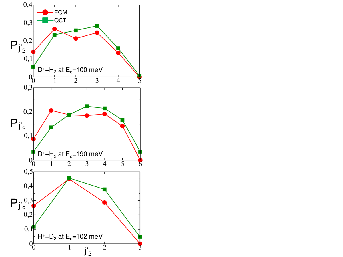
In this work, we focus on one of these shortcomings, namely the propensity of the standard QCT method to underestimate the populations of the less excited rotational states for the benefit of the most excited ones as compared to EQM results. This is clearly illustrated in Fig. 1 in the case of the D+ + H2 and H+ + D2 ion-molecule reactions (with the initial diatom in its rovibrational ground state), studied at collision energies sufficiently small for the product diatom HD to be in the vibrational ground state only. These distributions have been obtained by normalizing to unity the state-resolved integral cross sections (ICS) (see Eq. (2)) given in references [10] and [11] (see Fig. 6 in ref. [10] (upper panels) and Table II in ref. [11]). The same conclusion could be deduced from Fig. 6 in ref. [12] (upper panel; compare the GB-QCT and QM curves) or Figs. 17 and 20 in ref. [13] (the comparison is between QCT and experimental results there). This defect is problematic in the quantum regime where only a few rotational states (say, up to five or six) are available to the products, as is typically the case for endoergic reactions (like H+ + D2) at collision energies slightly above threshold.
Our goal in this paper is to find the cause and remedy of the previous limitation. This is a key issue regarding reactions for which EQM calculations are difficult to perform. In addition, the QCT method has a strong interpretative power. Therefore, improving its accuracy is also important when EQM calculations are feasible.
Since most benchmark quantum scattering calculations deal with triatomic reactions, we concentrate on these processes in the following.
The paper is organized as follows. In section II, we analyse the problem within the statistical framework of phase space theory (PST) [14, 15, 16, 17, 18, 19, 20, 21]. We then deduce the amendments to be introduced in classical PST (CPST) in order to make its predictions in exact agreement with those of quantum PST (QPST). These modifications are incorporated into the QCT method in section III. In particular, parity conservation is taken into account, for the first time in the QCT approach. The predictions of the resulting method are compared in section IV with EQM results and standard QCT ones in the case of the D+ + H2 and H+ + D2 reactions. Section V concludes.
II Classical vs Quantum PST
We consider the reaction A + BC AB + C. and are, respectively,
the vibrational and rotational quantum numbers of BC(AB). For simplicity’s sake, channel AC + B is supposed to be closed, and
both BC and AB are treated as rigid-rotor harmonic oscillators (RRHO).
The state-resolved ICS for the previous process reads [15, 17, 22]
| (1) |
is the linear momentum related to the reagent collision energy by , where is the reduced mass of A with respect to BC. is the total angular momentum quantum number and and are the reagent and product orbital angular momentum quantum numbers, respectively. is the probability to start from the reagents with at and , and reach the products with .
The population of product state is given in terms of by
| (2) |
where the sum in the denominator runs over all energetically accessible product states. For simplicity’s sake, will simply be denoted in the following, as the three remaining quantum numbers will be kept at 0 in the calculations.
In the present case, the reaction is supposed to involve a deep well along the reaction path where the system is trapped enough time for complete intramolecular redistribution of the available energy. In other words, the reaction proceeds through an intermediate complex “loosing the memory” of its initial conditions. Moreover, the dynamics in the entrance and exit-channels are assumed to be governed by isotropic long-range forces of the dispersion type. In such conditions, all the final states consistent with the conservation of total energy, total angular momentum, and parity, are equally likely. This is the basic assumption of PST.
Far in the reagent channel, the potential energy is given by
| (3) |
is the reduced mass of BC, is times its vibrational frequency, is the BC bond length, is its equilibrium value, is the distance between A and the center-of-mass of BC and is the reagent dipole-dipole dispersion coefficient which is assumed here to be the dominant one.
The internal energy of BC is given by
| (4) |
The total energy with respect to the bottom of the reagent channel is given by
| (5) |
while its analogue in the products reads
| (6) |
where is the exoergicity.
The potential energy far in the product channel and the internal energy of AB are given by the same expressions as Eqs. (3) and (4), with primed coordinates and parameters, and replaced by .
, the reduced mass of C with respect to AB, will appear later in the developments.
II.1 Quantum PST
Within the previous democratic assumption of equiprobable states, is given by
| (7) |
where is the probability that the system is captured in the well when coming from the reagents with at and , and is the probability that it reaches the products with , subject to conservation of total energy, and parity.
The capture probability is equal to 1 if
(i) the triangular inequality
| (8) |
is satisfied and
(ii) the centrifugal barrier height of the effective radial potential
| (9) |
is lower than the collision energy . Otherwise, is 0. This boolean choice is meaningful as tunneling through the centrifugal barrier is in practice negligible [18].
It may be shown that condition (ii) is equivalent to
| (10) |
with
| (11) |
[14, 16, 18]. is in fact the maximum value of the classical orbital angular momentum consistent
with capture at . Note that for not too small values of
, an excellent approximation of Eq. (10) is
| (12) |
From the microreversibility principle, products can only be reached with () (at and )
after exiting the well if the product capture probability is equal to 1.
The necessary conditions are the same as previously, but with product notations:
| (13) |
and
| (14) |
with
| (15) |
Here again, a very satisfying approximation of Eq. (14) is
| (16) |
However, these conditions alone do not warrant that state () is
available when coming from the reagents with (), and .
An additional condition is that parity conservation is satisfied [21], namely,
| (17) |
Defining the parity factor as
| (18) |
parity is conserved if , non conserved if .
The boolean number
| (19) |
then represents the actual contribution of to the whole set of available states.
The probability to reach from the well is then given by
| (20) |
where the sum in the denominator runs over all energetically accessible reactant and product states.
To set these ideas on a simple example, let us consider, for a hypothetical process, the case , , implying (see Eq. (8)), and assume that . For a given value of , the geometrical implications of the previously introduced constraints are depicted in Fig. 2. The brown “elliptic” curve is the upper bound of the partly visible grey area defined by energetic constraint (14). The rest of this area is hidden by the yellow area, defined by both the previous constraint and triangular inequality (13). This area is thus bounded by the brown curve and the three blue straight lines , and . The allowed states complying with the two previous constraints, and also parity constraint (17), are represented by green circles. Here, parity conservation forces the green states to satisfy . Prohibited states complying with the energetic constraint, triangular inequality, but violating parity conservation, are represented by red circles. For the green states, (both and are equal to 1) while for the red ones, ( but ). The checkerboard pattern formed by the green and red circles is the direct consequence of parity conservation.
II.2 Classical PST
What we call the CPST estimation of is its prediction from Eq. (1) with
calculated classical mechanically.
is then approximated by
| (21) |
where is the classical probability that the system is captured in the well when coming from the reagents with at and , and is the probability that a trajectory emmerging from the well contributes to the products in state , at and .
is equal to 1 if triangular inequality (8) is satisfied and if
| (22) |
(see previous section). Since the difference between and the right-hand-side (RHS) of Eq. (10) (see also Eq. (12)) is at most equal to 0.5, and are generally equal.
The process being statistical, is given by
| (23) |
where is the flux of trajectories exiting the well towards the products with and and contributing to state , is the total flux exiting the well towards the reagents with and and is the analogous flux towards the products. is the sum of over , and .
Convenient phase space coordinates for the mathematical formulation of the two previous fluxes [20] are two radial and ten action-angle coordinates. The radial coordinates are the distance between the center of mass of AB and atom C and its conjugate momentum . The ten action-angle coordinates are the total classical angular momentum , its projection on the -axis of the laboratory frame, their respective conjugate angles and , the vibrational action , the classical rotational angular momentum , the classical orbital angular momentum and their respective conjugate angles , and . These twelve coordinates form the phase space vector . From now on, will be expressed in unit and the angular momenta in unit. Analogous coordinates can be used in the reagents for the formulation of . More details on these coordinates can be found in ref. [20] and references therein.
Within the previous coordinate system, is given by [16, 20, 21]
| (24) |
is the function of Heaviside, equal to 1 if , 0 otherwise.
is the Dirac delta function. is the standard bin defined by
| (25) |
Assuming that any value of within the range contributes equally likely to the
vibrational quantum state , with the same type of assignment for and , is called
the standard binning (SB) procedure.
is an infinitely large value of . The classical Hamiltonian in the product channel reads
| (26) |
with
| (27) |
and
| (28) |
The superscript in and is to recall that these energies are classical, contrary to the quantum mechanical energies and (see Eqs. (9) and (4)).
II.3 Modifiying CPST so as to make it equivalent to QPST
Comparing Eqs. (7) and (21), the modification to perform in CPST in order to make it in
exact agreement with QPST should be such that, within the modified CPST,
| (31) |
and
| (32) |
or equivalently,
| (33) |
(see Eqs. (20) and (23)). These conditions will be fulfilled if the following method
is used:
(i) We replace the classical upper bound of (Eq. (22)) by its quantum analogue (Eq. (10)),
thus making identity (31) satisfied.
(ii) The functions in Eq. (29) are replaced by Gaussian functions of the type
| (34) |
normalized to unity, with tending to 0+.
Therefore, these Gaussians are equivalent to Dirac delta functions.
We may then integrate over in Eq. (29), thereby getting
| (35) |
being now equal to , the classical upper bound of is (see Eq. (30)).
(iii) We artificially impose in Eq. (35)
| (36) |
as an upper limit for . is given by Eq. (15) and
by Eq. (4) with ad-hoc product parameters.
This quantum boundary is compared with the classical boundary in Fig. 3 for
H+ + D2(0,0) at 102 meV, leading to D+ and HD in the vibrational ground state only.
The values of the parameters necessary to obtain these curves can be found in ref. [20].
When carefully looking at Eqs. (36), (15) and (4) (with product parameters) on the one hand,
and Eqs. (30) and (28) on the other hand, one arrives at the conclusion that one goes from the blue
to the red curve in Fig. 3 by replacing by
| (37) |
and by
| (38) |
approximated by and , respectively, for not too small values of or .
This observation will be useful later in this work.
The quantum limit is thus roughly shifted in by 0.5 with respect to the classical one along both
the and axes. In the present case, this shift plays a major role: the green states
in Fig. 3 are indeed
classically available, but quantally prohibited, thus implying that the rotational state population is 0 in QPST, but not in CPST.
(iv) Eq. (35) is now modified according to
| (39) |
is equal to 1 if lies below the red curve in Fig. 3, 0 if it lies
between the red and blue curves. Hence, makes 0 the contribution of the state consistent
with the classical capture but not the quantum one. As the basic reason responsible for the differences between the
classical and quantum capture limits is that the rotational energy associated with a given angular
momentum is slightly larger in classical than in quantum mechanics, we shall call the
rotational shift factor. Since the Gaussians are supposed to be infinitely narrow, one may rewrite Eq. (39) as
| (40) |
where is as previously defined, but for real values of and . This expression will appear to be useful in QCT calculations.
As previously discussed in section II.1, the parity factor makes the flux equal to 0 when parity conservation is not respected, but leaves unchanged the rest of the RHS of Eqs. (39) and (40) in the contrary case.
The remaining factor is defined by
| (41) |
where is the Kronecker symbol, equal to 1 if the two integers and are identical, 0 otherwise. We call it the edge factor for reasons that will appear obvious further below. For the example of section II.1, the bidimensional Gaussians centered at the available states (green circles in Fig. 2) are schematically represented in Fig. 4. A zoom of the Gaussian centered at (3,0) is also shown. Colored discs represent the areas where Gaussians take significant values. These areas have been arbitrarily increased for clarity’s sake, as we have previously assumed that tends to 0+, thereby implying that these areas tend to 0. For the magenta, orange and green Gaussians, 4, 2 and 1, respectively. Note that the substitution of the quantum boundaries of angular momenta to the classical values by means of the rotational shift factor makes the brown upper bounds in Figs. 2 and 4 rigorously identical. Otherwise, the upper bound in Fig. 4 would be roughly shifted out by one half (see Fig. 3).
We are now in a position to perform the integration over and in Eq. (39) for the example at hand. For corresponding to the two magenta Gaussians in Fig. 4, only one fourth of the Gaussians lie within the area imposed by the triangular inequality. This is clearly seen in the zoom of the Gaussian centered at (3,0). Hence, it is clear that their integration over and leads to one fourth. But for these Gaussians, . Consequently, . For the four orange Gaussians, half of the Gaussians lie within the previous area, but . The two remaining green Gaussians lie entirely within the area imposed by the triangular inequality, and . As a consequence, the edge factor makes for the eight Gaussians represented in Fig. 2, i.e., for the green states in Fig. 2. Moreover, is 0 for the red states in Fig. 2, due to the factor in Eq. (39). As a consequence, , such as given by Eq. (39), is proportional to and Eq. (32) is then satisfied (see also Eqs. (20) and (23)).
We now know that quantizing the vibrational, rotational and orbital motions by means of infinitely narrow Gaussians, and including the parity, edge and rotational shift factors in CPST makes it in exact agreement with QPST [23].
In order to illustrate this finding, the predictions of obtained by means of QPST and the modified CPST are represented in Fig. 5 for D+ + H2(0,0) at meV (red columns and blue diamonds, respectively). was kept at 0.06, a value for the which the full-width-at-half-maximum (FWHM) of the Gaussians is equal to 10. When used in QCT calculations, this procedure is commonly termed Gaussian binning (GB) [4, 10, 11, 12, 13, 24, 25, 26, 27, 28]. Below this value, the Monte-Carlo estimation of Eq. (40) starts getting harder to converge in a a few minutes, the usual amount of time required for QPST or CPST calculations. The values of the remaining parameters necessary to perform the PST calculations can be found in ref. [20]. As a matter of fact, the QPST and modified CPST predictions appear to be in excellent agreement. Note, however, that the modified CPST populations are slightly lower than the QPST ones. This is due to the fact that for the set of available quantum states very close to the brown upper bound in Fig. 2 or 4, the Gaussians partly overlap the forbiden region in the plane (unless tends to 0+). Their whole contribution is thus less than the number of previous states. But since the latter do not represent a large part of the whole set of available states, the above mentioned underestimation has only a minor impact on the final results.
III New implementation of the QCT method
The constraints previously introduced in CPST will now be included into the QCT approach, such as implemented in section 2 of ref.[4], or ref.[20].
In this method, action-angle coordinates such as those discussed in section II.2 are used to generate the initial conditions corresponding to the collision energy and the quantum numbers , , and appearing in the general expression (1) of the state-resolved ICS.
Like in most QCT approaches, trajectories are run
from a large initial distance , such that A and BC do not interact, with the radial momentum
| (42) |
(for not too large values of , the centrifugal energy may not be negligible as compared to ). The ten remaining action-angle coordinates to select are the total classical angular momentum, kept at , its projection on the -axis, kept at any value between and , their respective conjugate angles and , arbitrary, the vibrational action , taken at , the classical rotational angular momentum and the classical orbital angular momentum , respectively kept at and (see Eqs. (37) and (38)), and their conjugate angles , and , randomly chosen between 0 and . The last three angles at time 0 are collectively denoted . Note that taking at is equivalent to step (i) of the method proposed in section II.3.
To avoid any numerical instability, trajectories are run in Cartesian coordinates. The passage from , and the ten action-angle coordinates, to Cartesian ones, can be found in refs. [20, 29] (the similar transformation for polyatomic processes is given in ref. [30]). The product vibrational action, rotational angular momentum and orbital angular momentum are respectively denoted , and .
Following the developments of section 2 in ref.[4], the QCT expression of ,
including the modifications previously introduced in CPST (see steps (ii)-(iv) of the method proposed in section II.3)
reads
| (43) |
with
| (44) |
| (45) |
| (46) |
| (47) |
and
| (48) |
The practical calculation of the rotational shift factor is discussed further below. In Eq. (44), integration is made over the domain of initial angles leading to reactive trajectories. , in the first sum of the denominator of Eq. (43), is given by a similar expression involving non reactive trajectories. Note that is unitary, i.e., its sum over all energetically accessible reactant and product states leads to 1, as it should be.
Eq. (44), however, has a serious defect. The product of three narrow Gaussians in its integrand
makes the calculation very heavy. Using, for instance, Gaussians with
FWHM of 10 , only 0.1 of the trajectories do actually contribute to
[28]. Therefore, the calculations presented in the next section have been
performed by means of the GB procedure for the vibration motion only, while the SB procedure
has been used for the rotational and orbital angular motions. In this case,
| (49) |
with
| (50) |
and
| (51) |
(see Eq. (25)). This increases the number of efficient trajectories to 10 , a quite acceptable value.
The calculation of is as follows. We have seen in the previous section that one goes from the blue to the red curve in Fig. 3 by replacing and by and , respectively, in the analytical expression of the blue curve. was then kept at 1 below the red curve, and 0 between the red and blue curves. Note that was set equal to exactly. But it should be clear from Eqs. (14) and (15) that the red curve is also an upper bound of the area defined by the previous expressions and any value of larger than ( is indeed an increasing function of , and a decreasing one). Calling, respectively, and the rounded values of and , the idea is thus to find the maximum of for all the values of corresponding to the same , and analogously, the maximum of for all the values of corresponding to the same . From the previous remark on , all the trajectories leading to can be taken into account. is then kept at 1 if both and are lower than and , respectively, 0 otherwise. Finally, is kept at 0 for any value of larger than the maximum of the ’s.
was numerically estimated by randomly selecting and summing the integrand of Eq. (49). The number of trajectories run for each value of was chosen to be proportional to .
IV Application to the D+ + H2 and H+ + D2 reactions
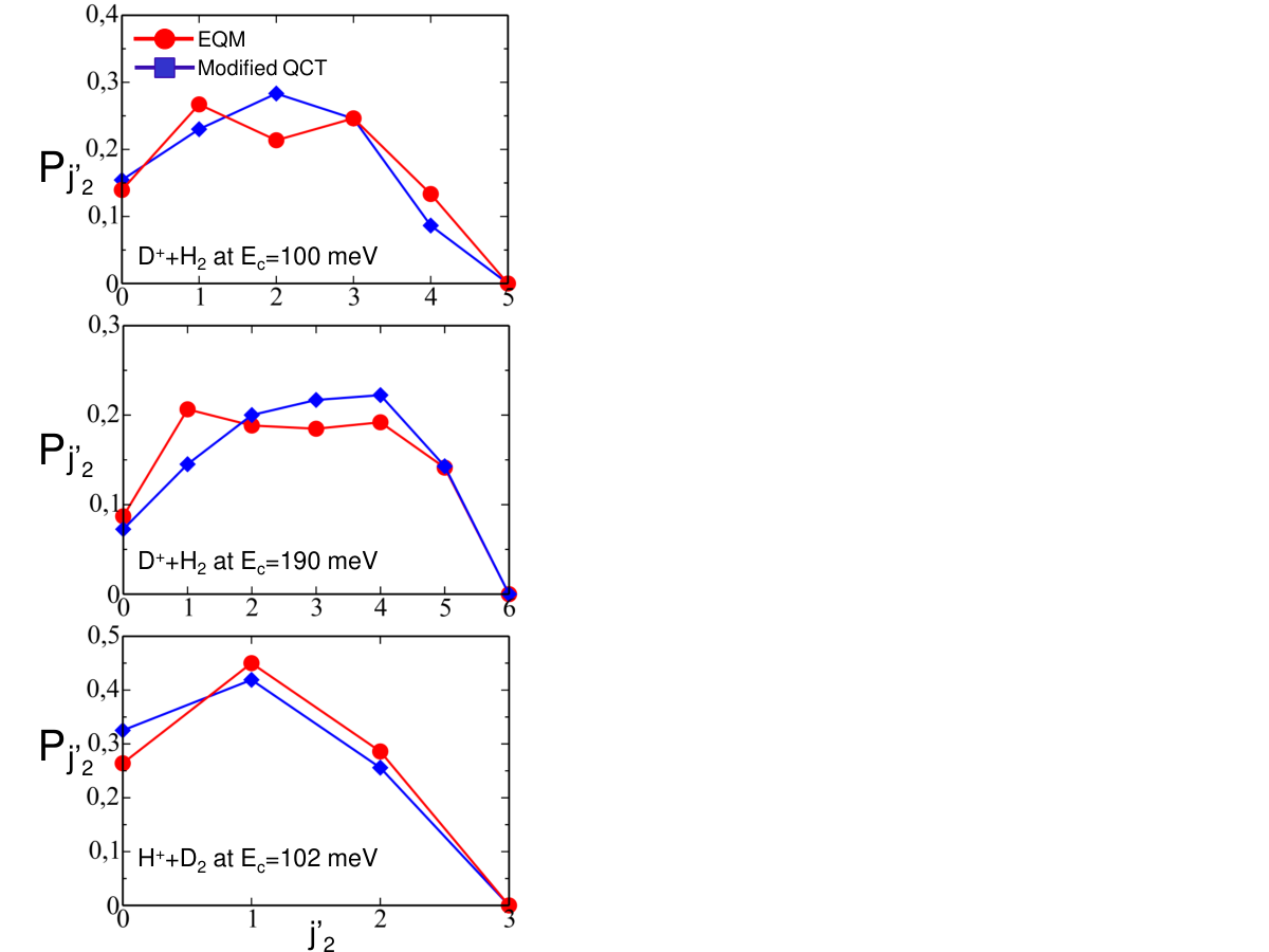
Batches of trajectories were run for (a) D+ + H2(0,0) at meV, (b) the same process at meV, and (c) H+ + D2(0,0) at meV. They were run on the same potential energy surface (PES) as in refs. [10] and [11], i.e., the PES of Aguado et al. [31]. Eqs. (1), (2) and (49) with lead to the blue diamonds in Fig. 6, to be compared with the red circles and the green squares in Fig. 1. Note that the latter have been found by using GB for , and SB for [10, 11]. As a matter of fact, the present QCT method leads to a much better prediction of than the standard QCT method. The former approach systematically enhances by a factor of compared to the latter. Consequently, the remaining populations are slightly decreased (except which is almost unchanged), thereby improving to some extent the overall shape of the rotational state distribution, especially for H+ + D2(0,0) in which only three states are available.
On the other hand, the modified (standard) QCT total ICS is found to be equal to 35.2 (28.2), 20.2 (22.8) and 15.4 (15.5) Å2 for reactions (a), (b) and (c), respectively, against 33.7, 27.6 and 23.6 Å2 from EQM calculations. Therefore, the modified QCT method only improves the ICS for reaction (a). For the remaining processes, both QCT methods tend to underestimate the ICS, a known defect studied in refs.[4] and [26], which precise origins remain to be clearly established.
V Conclusion
In the quantum regime where only a few rotational states are available to reaction products, the standard quasi-classical trajectory (QCT) method often underestimates the population of the less excited rotational states for the benefit of the most excited ones.
In the present work, we have analized the reasons for this underestimation in the light of the statistical phase space theory (PST) of chemical reactions. We have found three main sources of disagreement between classical PST (CPST) and quantum PST (QPST), and have introduced three related corrections making the modified CPST in agreement with QPST. These corrections consist in multiplying the final phase space states by a product of three factors, respectively called parity, edge and rotational shift factors, controlling to a large extent the shape of rotational state distributions.
These corrections have then been implemented in the QCT approach. For the ion-molecule reactions D+ + H2 and H+ + D2, the modified QCT prediction of the rotational ground state population turns out to be in much better agreement with the exact quantum mechanical one than the standard QCT prediction. The impact on the whole distribution is all the stronger as the number of available states is small.
The next steps are twofold: (i) checking that this improvement is general in the quantum regime by studying more processes and (ii) using this new QCT method to rationalize the shape of rotational state distributions in terms of energetic and mechanical parameters like collision energy, exoergicity, vibrational frequencies, atomic masses, etc…
Last but not least, this work is one more illustration of the fact that the QCT method may be much more accurate than expected two decades ago, provided that some quantum constraints are added to it in the light of the quantum and semiclassical formalisms. This is good news for polyatomic reactions which can rather easily be studied by the QCT method [13, 32], while hardly by EQM approaches.
References
- [1] R. Levine, Molecular Reaction Dynamics, Cambridge University Press, Cambridge, 2005.
- [2] R. N. Porter and L. M. Raff, in Dynamics of molecular collisions, Part B, edited by W. H. Miller, Plenum, New York, 1976.
- [3] T. D. Sewell and D. L. Thomson, Int. J. Mod. Phys. B, 11, 1067 (1997).
- [4] L. Bonnet, Int. Rev. Phys. Chem., 32, 171 (2013).
- [5] P. Honvault and J.-M. Launay, Theory of Chemical Reaction Dynamics (Kluwer Academic, Dordrecht, The Netherlands, 2004).
- [6] D. De Fazio, J. M. Lucas, V. Aquilanti and S. Cavalli, Phys. Chem. Chem. Phys. 13, 8571 (2011).
- [7] H. Guo, Int. Rev. Phys. Chem., 31, 1 (2012).
- [8] X. Yang, Phys. Chem. Chem. Phys. 13, 8112 (2011)
- [9] S. Chefdeville, Y. Kalugina, S. Y. T. van de Meerakker, C. Naulin, F. Lique and M. Costes, Science 341, 1094 (2013).
- [10] P. G. Jambrina, J. M. Alvariño, F. J. Aoiz, V. J. Herrero and V. Sãez-Rábanos, Phys. Chem. Chem. Phys., 12, 12591 (2010).
- [11] E. Carmona-Novillo, T. González-Lezana, O. Roncero, P. Honvault, J.-M. Launay, N. Bulut, F. J. Aoiz, L. Bañares, A. Trottier and E. Wrede, J. Chem. Phys., 128, 014304 (2008).
- [12] Z. Li, C. Xie, B. Jiang, D. Xie, L. Liu, Z. Sun, D.-H. Zhang and H. Guo, J. Chem. Phys., 134, 134303 (2011).
- [13] G. Czakó and J. M. Bowman, J. Phys. Chem. A, DOI: 10.1021/jp500085h.
- [14] P. Pechukas and J. C. Light, J. Chem. Phys., 42, 3281 (1965).
- [15] W. H. Miller, J. Chem. Phys., 52, 543 (1970).
- [16] L. Bonnet and J.-C. Rayez, Chem. Phys., 201, 203 (1995).
- [17] E. J. Rackham, F. Huarte-Larranaga, and D. E. Manolopoulos, Chem. Phys. Lett. 343, 356 (2001).
- [18] P. Larrégaray, L. Bonnet and J.-C. Rayez, J. Phys. Chem. A, 110, 1552 (2006).
- [19] T. Gonzalez-Lezana, Int. Rev. Phys. Chem. 26, 29 (2007).
- [20] L. Bonnet, P. Larrégaray, W. Arbelo-González and M. de Castro-Vítores, Comp. Theo. Chem., 990, 30 (2012).
- [21] L. Bonnet, P. Larrégaray and J.-C. Rayez, Phys. Chem. Chem. Phys., 9, 3228 (2007).
- [22] M. S. Child, Molecular Collision Theory, 1974, Academic Press.
- [23] We thought about making the change of momenta (,,)(,,) in Eq. (35) ( is also defined in terms of by a relation analogous to Eq. (37)). If in addition, one weights each state (,) by the inverse of the Jacobian of the transformation (,)(,), we arrive at the same integral as in Eq. (35), but with and replaced by and , respectively. The advantage of this change of variables is that the upper bounds of and are now the exact quantum mechanical ones, corresponding to the brown curve in Fig. 2, while those of and correspond to the red curve in Fig. 2. On the other hand, the serious drawback of this change of variables is that stricto sensu, , and do not satisfy the triangular inequality. Consequently, finding rules making exactly proportional to seems to be quite unobvious within the new coordinates (,). Therefore, we did not went further in that direction.
- [24] L. Bonnet and J.-C. Rayez, Chem. Phys. Lett., 277, 183 (1997).
- [25] L. Bonnet and J.-C. Rayez, Chem. Phys. Lett., 397, 106 (2004).
- [26] L. Bonnet, J. Chem. Phys., 128, 044109 (2008).
- [27] L. Bonnet, Chin. J. Chem. Phys., 22, 210 (2009).
- [28] L. Bonnet and J. Espinosa-Garcia, J. Chem. Phys., 133, 164108 (2010).
- [29] W. H. Miller, J. Chem. Phys., 54, 5386 (1971).
- [30] M. L. Gonzalez-Martinez, L. Bonnet, P. Larregaray, J.-C. Rayez and J. Rubayo-Soneira, J. Chem. Phys. 130, 114103 (2009).
- [31] A. Aguado, O. Roncero, C. Tablero, C. Sanz and M. Paniagua, J. Chem. Phys. 112, 1240 (2000).
- [32] E. Gonzalez-Lavado, J. C. Corchado and J. Espinosa-Garcia, J. Chem. Phys. 140, 064310 (2014).
Figures captions
Fig. 1: Distribution of the rotational quantum number of HD formed from the reactions D+ + H2
and H+ + D2. The initial diatom is in its rovibrational ground state. The values of the collision energy are
indicated. These are sufficiently low for HD to be in its vibrational ground state only.
Red circles and green squares correspond to exact quantum mechanical (EQM) and quasiclassical trajectory (QCT) results,
respectively. These distributions have been obtained by
normalizing to unity the state-resolved ICSs given in references [10] and [11].
, as well as for D+ + H2, appear to be underestimated by QCT compared to EQM.
Consequently, the remaining populations tend to be overestimated by QCT.
Fig. 2: Checkerboard pattern formed by allowed (green circles) and prohibited states (red circles)
in the plane for a hypothetical process, a given value of and . The partly visible grey
area represents the energetically available region while the yellow area is the part of the previous region
allowed by triangular inequality. Hence, the represented states satisfy energy and total angular momentum
requirements. Among them, however, only the green states comply with parity conservation
(see text for more details).
Fig. 3: Quantum upper bound (red curve) compared with its classical analogue (blue curve)
in the products of the reaction H+ + D2(0,0) at 102 meV.
The quantum limit is roughly shifted in by 0.5 with respect to the classical one along both
the and axes. The green states are classically available, but quantally prohibited.
is thus 0 in QPST, but not in CPST.
Fig. 4: For the process considered in Fig. 2, colored discs represent the areas where,
Gaussians centered at states
complying with triangular inequality and parity conservation, take significant values.
For the magenta, orange and green Gaussians, the edge factor is equal to 4, 2 and 1, respectively.
A zoom of the lowest magenta Gaussian is made in order to show that exactly one fourth of the Gaussian lies
within the yellow area allowed by the triangular inequality.
Fig. 5: Rotational state distribution obtained by means of QPST and the modified CPST
(red columns and blue diamonds, respectively). See text for more details on the calculations.
Figures