1Introduction

TTP14-011, SFB/CPP-14-22

On the gauge dependence of the

Standard Model vacuum instability scale

Luca Di Luzio and Luminita Mihaila
Institut für Theoretische Teilchenphysik, Karlsruhe Institute of Technology (KIT), D-76128 Karlsruhe, Germany

Abstract

After reviewing the calculation of the Standard Model one-loop effective potential in a class of linear gauges, we discuss the physical observables entering the vacuum stability analysis. While the electroweak-vacuum-stability bound on the Higgs boson mass can be formally proven to be gauge independent, the field value at which the effective potential turns negative (the so-called instability scale) is a gauge dependent quantity. By varying the gauge-fixing scheme and the gauge-fixing parameters in their perturbative domain, we find an irreducible theoretical uncertainty of at least two orders of magnitude on the scale at which the Standard Model vacuum becomes unstable.

1 Introduction

With the discovery of a Higgs-like boson at the LHC [1, 2], the question of the Standard Model (SM) vacuum stability has received a renewed attention, with several high-precision analysis on the subject [3, 4, 5, 6, 7, 8, 9, 10, 11] (see also [12, 13, 14, 15, 16, 17, 18, 19, 20, 21, 22, 23] for earlier works). Absolute vacuum stability bounds are usually obtained by requiring that the electroweak vacuum is the absolute minimum of the effective potential, at least up to some cutoff scale, $\Lambda_{\rm{SM}}$ , where the SM is not valid anymore and new physics is required in order to modify the shape of the effective potential.¹¹ 1 Such a requirement can be relaxed if the tunnelling probability of the electroweak vacuum is small enough to comply with the age of the universe. It would be tempting (as it is often done) to identify the physical threshold, $\Lambda_{\rm{SM}}$ , with the SM vacuum instability scale, $\Lambda$ , which is operatively defined by the field value at which the effective potential becomes deeper than the electroweak minimum. However, due to the gauge dependence of the effective potential, $\Lambda$ suffers from an irreducible gauge ambiguity which makes its identification with $\Lambda_{\rm{SM}}$ problematic.

The gauge dependence of the effective potential is known since long. Soon after the seminal work of Coleman and Weinberg [24], it was realized by Jackiw [25] that the effective potential is actually gauge dependent, thus raising the question of its physical significance. Since then, many authors have dealt with this subject [26, 27, 28, 29, 30, 31, 32, 33, 34, 35, 36, 37, 38, 39, 40] and it is now a well-established practice to extract the physical content of the effective potential by means of the so-called Nielsen identities [30].
In particular, the issue of the gauge dependence of the effective potential in the analysis of the SM vacuum stability was already pointed out at the end of the 90’s by Loinaz and Willey [41], which challenged the possibility of setting gauge-independent lower bounds on the Higgs boson mass from vacuum stability constraints. More recently, the problematic identification between the cutoff scale of the SM and the instability scale $\Lambda$ was mentioned again in Ref. [42].

The aim of this paper is to clarify some issues related to the gauge dependence of the quantities entering the vacuum stability analysis. While the critical value of the Higgs boson mass, marking the transition between the stable and unstable phase of the SM, can be formally proven to be gauge independent, the SM instability scale is actually gauge dependent. This is explicitly shown by a direct calculation of the gauge dependent one-loop effective potential in the SM.
The SM effective potential is known in the Landau gauge at one [24] and two loops [43, 44] since long. Recently, even the three-loop QCD and top-Yukawa corrections have been included [45]. On the other hand, calculations of the SM effective potential beyond the Landau gauge are less explored. Barring few exceptions, like for instance in Ref. [46] where a background-field-dependent gauge fixing with a single gauge-fixing parameter was employed, the gauge dependence of the SM effective potential is usually not taken into consideration.

The paper is organized as follows: in Sect. 2 we provide a pedagogical derivation of the SM one-loop effective potential in the Fermi gauge (generalized Lorentz gauge) and consider its renormalization group (RG) improvement. In Sect. 3 we discuss the physical observables entering the vacuum stability analysis. In particular, by using the Nielsen identity [30], we formally prove that the lower bound on the Higgs boson mass derived from the electroweak-vacuum-stability condition is gauge independent. On the other hand, the extrema of the effective potential and, in particular, the instability scale are in general gauge dependent. In Sect. 4 we numerically quantify at the next-to-leading order (NLO) accuracy the gauge dependence of $\Lambda$ in the Fermi gauge by varying the gauge-fixing parameters in their perturbative domain and comment on the gauge-fixing scheme dependence of $\Lambda$ . The interpretation and the physical implications of the gauge dependence of $\Lambda$ are discussed in Sect. 5. The two-loop renormalization group equations (RGEs) of the SM parameters in the Fermi gauge are collected in Appendix A, while in Appendix B we report on the calculation of the SM one-loop effective potential in a background $R_{\xi}$ gauge with the most general set of gauge-fixing parameters. As a by-product we also obtain the SM one-loop effective potential in the standard $R_{\xi}$ gauge, whose expression might be useful for broken-phase calculations.

2 The SM effective potential at one loop

In order to set the notation, let us split the classical Lagrangian density of the electroweak sector of the SM in a gauge, Higgs and fermion part

\mathcal{L}_{\rm{C}}=\mathcal{L}_{\rm{YM}}+\mathcal{L}_{\rm{H}}+\mathcal{L}_{\rm{F}}\,,

(1)

with

$\displaystyle\mathcal{L}_{\rm{YM}}$	$\displaystyle=-\frac{1}{4}\left(\partial_{\mu}W^{a}_{\nu}-\partial_{\nu}W^{a}_{\mu}+g\epsilon^{abc}W^{b}_{\mu}W^{c}_{\nu}\right)^{2}-\frac{1}{4}\left(\partial_{\mu}B_{\nu}-\partial_{\nu}B_{\mu}\right)^{2}\,,$	(2)
$\displaystyle\mathcal{L}_{\rm{H}}$	$\displaystyle=\left(D_{\mu}H\right)^{\dagger}\left(D^{\mu}H\right)-V(H)\,,$	(3)
$\displaystyle\mathcal{L}_{\rm{F}}$	$\displaystyle=\overline{Q}_{L}i\gamma_{\mu}D^{\mu}Q_{L}+\overline{t}_{R}i\gamma_{\mu}D^{\mu}t_{R}+\left(-y_{t}\overline{Q}_{L}(i\sigma^{2})H^{*}t_{R}+\rm{h.c.}\right)+\ldots\,,$	(4)

where $W^{a}_{\mu}$ ( $a=1,2,3$ ) and $B_{\mu}$ are the SU(2) and U(1) gauge fields, $H$ is the SM Higgs doublet with hypercharge $Y=1$ and $Q_{L}^{T}=(t_{L},b_{L})$ is the left-handed third generation quark doublet. Only the top quark is retained among the fermions and the QCD indices are suppressed in the quark sector. The covariant derivative is defined as

D_{\mu}=\partial_{\mu}-ig\frac{\sigma^{a}}{2}W^{a}_{\mu}+ig^{\prime}\frac{Y}{2}B_{\mu}\,,

(5)

where $\sigma^{a}$ ( $a=1,2,3$ ) are the usual Pauli matrices and with the term involving $g$ being absent for right-handed fermions. The Higgs potential is

V(H)=-m^{2}H^{\dagger}H+\lambda(H^{\dagger}H)^{2}\,.

(6)

The effective potential can be conveniently computed by means of the background field method of Jackiw [25]. After homogeneously shifting the scalar fields of the theory by a background (spacetime independent) field $\phi$ , the one-loop effective potential is obtained by directly evaluating the path integral expression of the effective action in the Gaussian approximation. After some standard manipulations (see e.g. also [47, 46]), the one-loop effective potential

V_{\rm{eff}}^{\rm{1-loop}}(\phi)=V^{(0)}_{\rm{eff}}(\phi)+V^{(1)}_{\rm{eff}}(\phi)\,,

(7)

can be recast in terms of the well-known formulas [25]

	$\displaystyle V^{(0)}_{\rm{eff}}(\phi)$	$\displaystyle=V(\phi)\,,$		(8)
	$\displaystyle V^{(1)}_{\rm{eff}}(\phi)$	$\displaystyle=i\sum_{n\,=\,\text{SM fields}}\eta\int\frac{d^{4}k}{(2\pi)^{4}}\log\mbox{det}\,i\tilde{\mathcal{D}}^{-1}_{n}\{\phi;k\}\,.$		(9)

The matrix $i\tilde{\mathcal{D}}^{-1}_{n}\{\phi;k\}$ denotes the $\phi$ -dependent inverse propagators of the SM fields in momentum space, the determinant acts on all the internal indices and $\eta=-1/2\ (1)$ for bosons (fermions/ghosts) is the power of the functional determinant due to the Gaussian path integral.

Gauge invariance allows us to perform the shift of the Higgs doublet in a specific direction of the $\rm{SU(2)}\otimes\rm{U(1)}$ space:

H(x)\rightarrow\frac{1}{\sqrt{2}}\left(\begin{array}[]{c}\chi^{1}(x)+i\chi^{2}(x)\\ \phi+h(x)+i\chi^{3}(x)\end{array}\right)\,,

(10)

where $h$ denotes the Higgs field and $\chi^{a}$ ( $a=1,2,3$ ) the Goldstone boson fields. At tree level, the effective potential reads

V^{(0)}_{\rm{eff}}(\phi)=-\frac{m^{2}}{2}\phi^{2}+\frac{\lambda}{4}\phi^{4}\,,

(11)

while in order to compute the quantum correction, $V^{(1)}_{\rm{eff}}$ , one needs to work out the inverse propagators of the dynamical fields in the shifted SM Lagrangian. For exemplification, we consider in the next section the computation of the one-loop SM effective potential in the Fermi gauge. The calculation of the SM effective potential in a background-field-dependent $R_{\xi}$ gauge and in the standard $R_{\xi}$ gauge is instead presented in Appendix B.

2.1 Fermi gauge

As long as we are interested in the high-energy behaviour of the the effective potential, we can directly work in the unbroken phase of the SM. Then, the most convenient way to fix the gauge is by means of the Fermi gauge (generalized Lorentz gauge):

\mathcal{L}^{\rm{Fermi}}_{\rm{g.f.}}=-\frac{1}{2\xi_{W}}\left(\partial^{\mu}W^{a}_{\mu}\right)^{2}-\frac{1}{2\xi_{B}}\left(\partial^{\mu}B_{\mu}\right)^{2}\,.

(12)

We are thus interested in the determination of the quadratic ( $\phi$ -dependent) part of the Lagrangian, $\mathcal{L}_{\rm{C}}+\mathcal{L}^{\rm{Fermi}}_{\rm{g.f.}}$ , after the shift in Eq. (10).²² 2 One can easily see that the bilinear ghost terms are $\phi$ -independent. Hence, in the Fermi gauge the ghost contribution decouples from the one-loop effective potential. A straightforward calculation yields

$\displaystyle\mathcal{L}^{\rm{quad}}_{\rm{YM}}$	$\displaystyle=\tfrac{1}{2}W^{a}_{\mu}\left(\Box\,g^{\mu\nu}-\partial^{\mu}\partial^{\nu}\right)\delta^{ab}W^{b}_{\nu}+\tfrac{1}{2}B_{\mu}\left(\Box\,g^{\mu\nu}-\partial^{\mu}\partial^{\nu}\right)B_{\nu}\,,$	(13)
$\displaystyle\mathcal{L}^{\rm{quad}}_{\rm{H}}$	$\displaystyle=\tfrac{1}{2}h\left(-\Box-\bar{m}_{h}^{2}\right)h+\tfrac{1}{2}\chi^{a}\left(-\Box-\bar{m}_{\chi}^{2}\right)\delta^{ab}\chi^{b}+\tfrac{1}{2}\bar{m}_{W}^{2}W^{a}_{\mu}W^{a\mu}+\tfrac{1}{2}\bar{m}_{B}^{2}B_{\mu}B^{\mu}$
	$\displaystyle+\bar{m}_{W}\bar{m}_{B}W^{3}_{\mu}B^{\mu}-\bar{m}_{W}\partial_{\mu}\chi^{1}W^{2\mu}-\bar{m}_{W}\partial_{\mu}\chi^{2}W^{1\mu}+\bar{m}_{W}\partial_{\mu}\chi^{3}W^{3\mu}+\bar{m}_{B}\partial_{\mu}\chi^{3}B^{\mu}\,,$	(14)
$\displaystyle\mathcal{L}^{\rm{quad}}_{\rm{F}}$	$\displaystyle=\overline{t}\left(i\not{\partial}-\bar{m}_{t}\right)t+\ldots\,,$	(15)

where $\Box\equiv\partial_{\mu}\partial^{\mu}$ and we defined the $\phi$ -dependent masses

$\displaystyle\bar{m}_{h}^{2}$	$\displaystyle=-m^{2}+3\lambda\phi^{2}\,,$	(16)
$\displaystyle\bar{m}_{\chi}^{2}$	$\displaystyle=-m^{2}+\lambda\phi^{2}\,,$	(17)
$\displaystyle\bar{m}_{W}$	$\displaystyle=\tfrac{1}{2}g\phi\,,$	(18)
$\displaystyle\bar{m}_{B}$	$\displaystyle=\tfrac{1}{2}g^{\prime}\phi\,,$	(19)
$\displaystyle\bar{m}_{t}$	$\displaystyle=\frac{y_{t}}{\sqrt{2}}\phi\,,$	(20)

while $\mathcal{L}^{\rm{Fermi}}_{\rm{g.f.}}$ is already quadratic in the gauge boson fields. The only technical complication in the Fermi gauge is the presence of a Goldstone–gauge boson mixing already at tree level (cf. Eq. (14)). The latter can be treated by defining an extended field vector

X^{T}=\left(V^{T}_{\mu},\chi^{T}\right)\,,

(21)

where

V^{T}_{\mu}=\left(W^{1}_{\mu},W^{2}_{\mu},W^{3}_{\mu},B_{\mu}\right)\,,\qquad\chi^{T}=\left(\chi^{1},\chi^{2},\chi^{3}\right)\,.

(22)

Then the quadratic part of the Goldstone–gauge sector can be rewritten as

\frac{1}{2}X^{T}\left(i\mathcal{D}_{X}^{-1}\right)X=\frac{1}{2}\left(V_{\mu}^{T},\chi^{T}\right)\left(\begin{array}[]{cc}i\left(\mathcal{D}^{-1}_{V}\right)^{\mu}_{\nu}&\bar{m}^{T}_{\text{mix}}\,\partial^{\mu}\\ -\bar{m}_{\text{mix}}\,\partial_{\nu}&i\mathcal{D}^{-1}_{\chi}\end{array}\right)\left(\begin{array}[]{c}V^{\nu}\\ \chi\end{array}\right)\,,

(23)

with

\bar{m}_{\text{mix}}=\left(\begin{array}[]{cccc}0&-\bar{m}_{W}&0&0\\ -\bar{m}_{W}&0&0&0\\ 0&0&\bar{m}_{W}&\bar{m}_{B}\end{array}\right)\,.

(24)

After Fourier transformation, $\partial_{\mu}\rightarrow ik_{\mu}$ , the mixed inverse propagator matrix becomes

i\tilde{\mathcal{D}}_{X}^{-1}=\left(\begin{array}[]{cc}i(\tilde{\mathcal{D}}^{-1}_{V})^{\mu}_{\nu}&ik^{\mu}\bar{m}^{T}_{\text{mix}}\\ -ik_{\nu}\bar{m}_{\text{mix}}&i\tilde{\mathcal{D}}^{-1}_{\chi}\end{array}\right)\,,

(25)

where $(\tilde{\mathcal{D}}^{-1}_{V})^{\mu}_{\nu}$ is conveniently split into a transversal and a longitudinal part

(\tilde{\mathcal{D}}^{-1}_{V})^{\mu}_{\nu}=i\tilde{\mathcal{D}}^{-1}_{T}\,(\Pi_{T})^{\mu}_{\nu}+i\tilde{\mathcal{D}}^{-1}_{L}\,(\Pi_{L})^{\mu}_{\nu}\,,

(26)

with

(\Pi_{T})^{\mu}_{\nu}=g^{\mu}_{\nu}-\frac{k^{\mu}k_{\nu}}{k^{2}}\,,\qquad(\Pi_{L})^{\mu}_{\nu}=\frac{k^{\mu}k_{\nu}}{k^{2}}\,,

(27)

and

	$\displaystyle i\tilde{\mathcal{D}}^{-1}_{T}$	$\displaystyle=\left(\begin{array}[]{cccc}-k^{2}+\bar{m}_{W}^{2}&0&0&0\\ 0&-k^{2}+\bar{m}_{W}^{2}&0&0\\ 0&0&-k^{2}+\bar{m}_{W}^{2}&\bar{m}_{W}\bar{m}_{B}\\ 0&0&\bar{m}_{W}\bar{m}_{B}&-k^{2}+\bar{m}_{B}^{2}\end{array}\right)\,,$
	$\displaystyle i\tilde{\mathcal{D}}^{-1}_{L}$	$\displaystyle=\left(\begin{array}[]{cccc}-\xi_{W}^{-1}k^{2}+\bar{m}_{W}^{2}&0&0&0\\ 0&-\xi_{W}^{-1}k^{2}+\bar{m}_{W}^{2}&0&0\\ 0&0&-\xi_{W}^{-1}k^{2}+\bar{m}_{W}^{2}&\bar{m}_{W}\bar{m}_{B}\\ 0&0&\bar{m}_{W}\bar{m}_{B}&-\xi_{B}^{-1}k^{2}+\bar{m}_{B}^{2}\end{array}\right)\,.$

The Goldstone boson inverse propagator reads

i\tilde{\mathcal{D}}^{-1}_{\chi}=\left(\begin{array}[]{ccc}k^{2}-\bar{m}_{\chi}^{2}&0&0\\ 0&k^{2}-\bar{m}_{\chi}^{2}&0\\ 0&0&k^{2}-\bar{m}_{\chi}^{2}\end{array}\right)\,,

(36)

while those of the Higgs and top quark fields are

	$\displaystyle i\tilde{\mathcal{D}}^{-1}_{h}$	$\displaystyle=k^{2}-\bar{m}_{h}^{2}\,,$		(37)
	$\displaystyle i\tilde{\mathcal{D}}^{-1}_{t}$	$\displaystyle=\not{k}-\bar{m}_{t}\,.$		(38)

The next step (see Eq. (9)) is the evaluation of $\log\mbox{det}\,i\tilde{\mathcal{D}}_{n}^{-1}$ , for $n=X,h,t$ . Only the former and the latter present some non-trivial steps. Let us start by expressing the determinant of the block matrix in Eq. (25) as

	$\displaystyle\mbox{det}\,i\tilde{\mathcal{D}}_{X}^{-1}$	$\displaystyle=\mbox{det}\,i\tilde{\mathcal{D}}_{\chi}^{-1}\mbox{det}\,\left(i(\tilde{\mathcal{D}}^{-1}_{V})^{\mu}_{\nu}-k^{\mu}k_{\nu}\bar{m}^{T}_{\text{mix}}\left(i\tilde{\mathcal{D}}^{-1}_{\chi}\right)^{-1}\bar{m}_{\text{mix}}\right)\,,$
		$\displaystyle=\mbox{det}\,i\tilde{\mathcal{D}}_{\chi}^{-1}\mbox{det}\,\left(i\tilde{\mathcal{D}}^{-1}_{T}(\Pi_{T})^{\mu}_{\nu}+\left(i\tilde{\mathcal{D}}^{-1}_{L}-k^{2}\bar{m}^{T}_{\text{mix}}\left(i\tilde{\mathcal{D}}^{-1}_{\chi}\right)^{-1}\bar{m}_{\text{mix}}\right)(\Pi_{L})^{\mu}_{\nu}\right)\,,$		(39)

where in the last step we used Eq. (26), and perform a Lorentz transformation in $d$ spacetime dimensions,³³ 3 We already anticipate the fact that we are going to regulate the divergent integrals in dimensional regularization. $k_{\mu}\rightarrow(k_{0},0,0,0,\ldots)$ , such that $(\Pi_{L})^{\mu}_{\nu}\rightarrow(1,0,0,0,\ldots)$ and $(\Pi_{T})^{\mu}_{\nu}\rightarrow(0,1,1,1,\ldots)$ . Using the Loretz invariance of the determinant, we obtain

\log\mbox{det}\,i\tilde{\mathcal{D}}_{X}^{-1}=(d-1)\log\mbox{det}\,\tilde{\mathcal{D}}^{-1}_{T}+\log\mbox{det}\,i\tilde{\mathcal{D}}_{\chi}^{-1}\mbox{det}\,\left(i\tilde{\mathcal{D}}^{-1}_{L}-k^{2}\bar{m}^{T}_{\text{mix}}\left(i\tilde{\mathcal{D}}^{-1}_{\chi}\right)^{-1}\bar{m}_{\text{mix}}\right)\,.

(40)

The explicit evaluation of the two summands in the right-hand side of Eq. (40) yields

\log\mbox{det}\,i\tilde{\mathcal{D}}^{-1}_{T}=2\log\left(-k^{2}+\bar{m}_{W}^{2}\right)+\log\left(-k^{2}+\bar{m}_{Z}^{2}\right)+\ldots\,,\\

(41)

and

		$\displaystyle\log\mbox{det}\,i\tilde{\mathcal{D}}_{\chi}^{-1}\mbox{det}\,\left(i\tilde{\mathcal{D}}^{-1}_{L}-k^{2}\bar{m}^{T}_{\text{mix}}\left(i\tilde{\mathcal{D}}^{-1}_{\chi}\right)^{-1}\bar{m}_{\text{mix}}\right)$
		$\displaystyle=2\log\left(k^{4}-k^{2}\bar{m}_{\chi}^{2}+\bar{m}_{\chi}^{2}\xi_{W}\bar{m}_{W}^{2}\right)+\log\left(k^{4}-k^{2}\bar{m}_{\chi}^{2}+\bar{m}_{\chi}^{2}(\xi_{W}\bar{m}_{W}^{2}+\xi_{B}\bar{m}_{B}^{2})\right)+\ldots$
		$\displaystyle=2\log\left(k^{2}-\bar{m}_{A^{+}}^{2}\right)+2\log\left(k^{2}-\bar{m}_{A^{-}}^{2}\right)+\log\left(k^{2}-\bar{m}_{B^{+}}^{2}\right)+\log\left(k^{2}-\bar{m}_{B^{-}}^{2}\right)+\ldots\,,$		(42)

where the ellipses stand for $\phi$ -independent terms and we defined the $\phi$ -dependent masses

$\displaystyle\bar{m}_{Z}^{2}$	$\displaystyle=\bar{m}_{W}^{2}+\bar{m}_{B}^{2}\,,$	(43)
$\displaystyle\bar{m}_{A^{\pm}}^{2}$	$\displaystyle=\frac{1}{2}\bar{m}_{\chi}\left(\bar{m}_{\chi}\pm\sqrt{\bar{m}_{\chi}^{2}-4\xi_{W}\bar{m}_{W}^{2}}\right)\,,$	(44)
$\displaystyle\bar{m}_{B^{\pm}}^{2}$	$\displaystyle=\frac{1}{2}\bar{m}_{\chi}\left(\bar{m}_{\chi}\pm\sqrt{\bar{m}_{\chi}^{2}-4(\xi_{W}\bar{m}_{W}^{2}+\xi_{B}\bar{m}_{B}^{2})}\right)\,.$	(45)

For the evaluation of the fermionic determinant of Eq. (38) we employ a naive treatment of $\gamma_{5}$ in dimensional regularization (i.e. $\{\gamma_{5},\gamma_{\mu}\}=0$ in $d$ dimensions) and make the standard choice $\mbox{Tr}\,\mathbf{1}_{\text{Dirac}}=4$ in $d$ dimensions.⁴⁴ 4 A different choice, e.g. $\mbox{Tr}\,\mathbf{1}_{\text{Dirac}}=2^{d/2}$ , would just lead to a different renormalization scheme [48]. Explicitly, one has

$\displaystyle\log\mbox{det}\,\left(\not{k}-\bar{m}_{t}\right)$	$\displaystyle=\mbox{Tr}\,\log\left(\not{k}-\bar{m}_{t}\right)=\mbox{Tr}\,\log\gamma^{5}\left(\not{k}-\bar{m}_{t}\right)\gamma^{5}=\mbox{Tr}\,\log\left(-\not{k}-\bar{m}_{t}\right)$
	$\displaystyle=\frac{1}{2}\left[\mbox{Tr}\,\log\left(\not{k}-\bar{m}_{t}\right)+\mbox{Tr}\,\log\left(-\not{k}-\bar{m}_{t}\right)\right]=\frac{1}{2}\mbox{Tr}\,\log\left(-k^{2}+\bar{m}_{t}^{2}\right)$
	$\displaystyle=\frac{1}{2}4\times 3\log\left(-k^{2}+\bar{m}_{t}^{2}\right)\,,$	(46)

where the extra factors in the last step are due to the trace in the Dirac and color space.

Including all the relevant degrees of freedom and working in dimensional regularization with $d=4-2\epsilon$ , the one-loop contribution to the effective potential (cf. again Eq. (9)) can be adjusted in the following way:

$\displaystyle V^{(1)}_{\rm{eff}}(\phi)\|^{\rm{Fermi}}$	$\displaystyle=-\frac{i}{2}\mu^{2\epsilon}\int\frac{d^{d}k}{(2\pi)^{d}}\left[-12\log\left(-k^{2}+\bar{m}_{t}^{2}\right)+(d-1)\left(2\log\left(-k^{2}+\bar{m}_{W}^{2}\right)\right.\right.$
	$\displaystyle\left.+\log\left(-k^{2}+\bar{m}_{Z}^{2}\right)\right)+\log\left(k^{2}-\bar{m}_{h}^{2}\right)+2\log\left(k^{2}-\bar{m}_{A^{+}}^{2}\right)+2\log\left(k^{2}-\bar{m}_{A^{-}}^{2}\right)$
	$\displaystyle\left.+\log\left(k^{2}-\bar{m}_{B^{+}}^{2}\right)+\log\left(k^{2}-\bar{m}_{B^{-}}^{2}\right)+\ \text{$\phi$-independent}\right]\,.$	(47)

The integrals are easily evaluated after Wick rotation, yielding

-\frac{i}{2}\mu^{2\epsilon}\int\frac{d^{d}k}{(2\pi)^{d}}\log(-k^{2}+m^{2})=\frac{1}{4}\frac{m^{4}}{(4\pi)^{2}}\left(\log\frac{m^{2}}{\mu^{2}}-\frac{3}{2}-\Delta_{\epsilon}\right)\,,

(48)

where we introduced the modified minimal subtraction ( $\overline{\rm{MS}}$ ) term [49]

\Delta_{\epsilon}=\frac{1}{\epsilon}-\gamma_{E}+\log 4\pi\,.

(49)

After the $\epsilon$ -expansion the one-loop contribution to the effective potential is given by

		$\displaystyle V^{(1)}_{\rm{eff}}\|_{\rm{bare}}^{\rm{Fermi}}=\frac{1}{4(4\pi)^{2}}\left[-12\bar{m}_{t}^{4}\left(\log\frac{\bar{m}_{t}^{2}}{\mu^{2}}-\frac{3}{2}-\Delta_{\epsilon}\right)+6\bar{m}_{W}^{4}\left(\log\frac{\bar{m}_{W}^{2}}{\mu^{2}}-\frac{5}{6}-\Delta_{\epsilon}\right)\right.$		(50)
		$\displaystyle\left.+3\bar{m}_{Z}^{4}\left(\log\frac{\bar{m}_{Z}^{2}}{\mu^{2}}-\frac{5}{6}-\Delta_{\epsilon}\right)+\bar{m}_{h}^{4}\left(\log\frac{\bar{m}_{h}^{2}}{\mu^{2}}-\frac{3}{2}-\Delta_{\epsilon}\right)+2\bar{m}_{A^{+}}^{4}\left(\log\frac{\bar{m}_{A^{+}}^{2}}{\mu^{2}}-\frac{3}{2}-\Delta_{\epsilon}\right)\right.$
		$\displaystyle\left.+2\bar{m}_{A^{-}}^{4}\left(\log\frac{\bar{m}_{A^{-}}^{2}}{\mu^{2}}-\frac{3}{2}-\Delta_{\epsilon}\right)+\bar{m}_{B^{+}}^{4}\left(\log\frac{\bar{m}_{B^{+}}^{2}}{\mu^{2}}-\frac{3}{2}-\Delta_{\epsilon}\right)+\bar{m}_{B^{-}}^{4}\left(\log\frac{\bar{m}_{B^{-}}^{2}}{\mu^{2}}-\frac{3}{2}-\Delta_{\epsilon}\right)\right]\,.$

In particular, in terms of the SM couplings the divergent part of Eq. (50) reads

	$\displaystyle V^{(1)}_{\rm{eff}}\|_{\rm{bare-pole}}^{\rm{Fermi}}$	$\displaystyle=\frac{\Delta_{\epsilon}}{(4\pi)^{2}}\left[-m^{4}+\left(3\lambda-\frac{1}{8}\xi_{B}g^{\prime 2}-\frac{3}{8}\xi_{W}g^{2}\right)m^{2}\phi^{2}\right.$
		$\displaystyle\left.+\left(-\frac{3}{64}g^{\prime 4}-\frac{3}{32}g^{\prime 2}g^{2}-\frac{9}{64}g^{4}+\frac{3}{4}y_{t}^{4}-3\lambda^{2}+\frac{1}{8}\xi_{B}g^{\prime 2}\lambda+\frac{3}{8}\xi_{W}g^{2}\lambda\right)\phi^{4}\right]\,.$		(51)

While the $m^{4}$ -dependent pole in Eq. (51) can be always subtracted by a constant shift in the effective potential,⁵⁵ 5 A constant shift in the effective potential does not affect the equations of motion, as long as gravity is ignored. the remaining divergences are canceled by the multiplicative renormalization of the bare field and couplings appearing in $V^{(0)}_{\rm{eff}}$ (cf. Eq. (11)):

\phi_{0}=Z_{\phi}^{1/2}|^{\rm{Fermi}}\phi\,,\qquad m^{2}_{0}=Z_{m^{2}}m^{2}\,,\qquad\lambda_{0}=Z_{\lambda}\lambda\,,

(52)

where the renormalization constants can be conveniently computed in the unbroken phase of the SM. Their expressions at one loop in the $\overline{\rm{MS}}$ scheme read (see e.g. [50, 51]):

$\displaystyle Z_{\phi}^{1/2}\|^{\rm{Fermi}}$	$\displaystyle=1+\frac{\Delta_{\epsilon}}{(4\pi)^{2}}\left(\frac{3}{8}g^{\prime 2}+\frac{9}{8}g^{2}-\frac{3}{2}y_{t}^{2}-\frac{1}{8}\xi_{B}g^{\prime 2}-\frac{3}{8}\xi_{W}g^{2}\right)\,,$	(53)
$\displaystyle Z_{m^{2}}$	$\displaystyle=1+\frac{\Delta_{\epsilon}}{(4\pi)^{2}}\left(-\frac{3}{4}g^{\prime 2}-\frac{9}{4}g^{2}+3y_{t}^{2}+6\lambda\right)\,,$	(54)
$\displaystyle Z_{\lambda}$	$\displaystyle=1+\frac{\Delta_{\epsilon}}{(4\pi)^{2}}\left(-\frac{3}{2}g^{\prime 2}-\frac{9}{2}g^{2}+6y_{t}^{2}+12\lambda+\frac{3}{16}\frac{g^{\prime 4}}{\lambda}+\frac{3}{8}\frac{g^{\prime 2}g^{2}}{\lambda}+\frac{9}{16}\frac{g^{4}}{\lambda}-3\frac{y_{t}^{4}}{\lambda}\right)\,.$	(55)

It is a simple exercise to check that the renormalization of the tree-level potential, via the renormalization constants in Eqs. (53)–(55), cancels the $\phi$ -dependent poles in Eq. (51). Let us point out that in the Fermi gauge the field $\phi$ gets only multiplicatively renormalized by the wavefunction of the Higgs field. This feature is due to the invariance of the complete SM Lagrangian (including the gauge-fixing term in Eq. (12)) under the transformation $h\rightarrow h+a$ and $\phi\rightarrow\phi-a$ , as shown in [52, 53]. As we will see in Appendix B, this property does not hold anymore in the background $R_{\xi}$ gauge.

Hence, after the renormalization procedure, the one-loop contribution to the effective potential in the $\overline{\rm{MS}}$ scheme reads

$\displaystyle V^{(1)}_{\rm{eff}}\|^{\rm{Fermi}}$	$\displaystyle=\frac{1}{4(4\pi)^{2}}\left[-12\bar{m}_{t}^{4}\left(\log\frac{\bar{m}_{t}^{2}}{\mu^{2}}-\frac{3}{2}\right)+6\bar{m}_{W}^{4}\left(\log\frac{\bar{m}_{W}^{2}}{\mu^{2}}-\frac{5}{6}\right)\right.$
	$\displaystyle\left.+3\bar{m}_{Z}^{4}\left(\log\frac{\bar{m}_{Z}^{2}}{\mu^{2}}-\frac{5}{6}\right)+\bar{m}_{h}^{4}\left(\log\frac{\bar{m}_{h}^{2}}{\mu^{2}}-\frac{3}{2}\right)+2\bar{m}_{A^{+}}^{4}\left(\log\frac{\bar{m}_{A^{+}}^{2}}{\mu^{2}}-\frac{3}{2}\right)\right.$
	$\displaystyle\left.+2\bar{m}_{A^{-}}^{4}\left(\log\frac{\bar{m}_{A^{-}}^{2}}{\mu^{2}}-\frac{3}{2}\right)+\bar{m}_{B^{+}}^{4}\left(\log\frac{\bar{m}_{B^{+}}^{2}}{\mu^{2}}-\frac{3}{2}\right)+\bar{m}_{B^{-}}^{4}\left(\log\frac{\bar{m}_{B^{-}}^{2}}{\mu^{2}}-\frac{3}{2}\right)\right]\,,$	(56)

where the definitions of the $\phi$ -dependent mass terms are given in Eqs. (16)–(20) and Eqs. (43)–(45). In particular, for $\xi_{W}=\xi_{B}=0$ one has $\bar{m}_{A^{+}}=\bar{m}_{B^{+}}=\bar{m}_{\chi}$ and $\bar{m}_{A^{-}}=\bar{m}_{B^{-}}=0$ , so that Eq. (56) reproduces the standard one-loop result in the Landau gauge [24].

Let us stress that the gauge dependence of $V^{(1)}_{\rm{eff}}$ cannot be removed by a suitable choice of the renormalization scheme, as it can be verified by adding finite terms in Eqs. (53)–(55). Notice, however, that on the tree-level minimum, $m^{2}=\lambda\phi^{2}$ (hence $\bar{m}_{\chi}=0$ and $\bar{m}_{A^{\pm}}=\bar{m}_{B^{\pm}}=0$ ), the gauge dependence drops from $V^{(1)}_{\rm{eff}}|^{\rm{Fermi}}$ . We will discuss this aspect in more detail in Sect. 3.

2.2 Renormalization group improvement

In applications where the behavior of $V_{\rm{eff}}(\phi)$ at large $\phi$ is needed, like for the vacuum stability analysis, one has to deal with potentially large logarithms of the type $\log(\phi/\mu)$ which may spoil the applicability range of perturbation theory. The standard way to resum such logarithms is by means of the RGEs. Since $V_{\rm{eff}}$ is independent of the renormalization scale $\mu$ for fixed values of the bare parameters, one obtains the RGE

\left(\mu\frac{\partial}{\partial\mu}+\beta_{i}\frac{\partial}{\partial\lambda_{i}}-\gamma\phi\frac{\partial}{\partial\phi}\right)V_{\rm{eff}}=0\,,

(57)

where the beta functions

\beta_{i}=\mu\frac{d\lambda_{i}}{d\mu}\,,

(58)

correspond to each of the SM coupling $\lambda_{i}$ (including the gauge-fixing parameters) and the anomalous dimension of the background field is defined by

\gamma=-\frac{\mu}{\phi}\frac{d\phi}{d\mu}\,.

(59)

The formal solution of the RGE in Eq. (57) can be obtained by applying the method of the characteristics [16]:

V_{\rm{eff}}(\mu,\lambda_{i},\phi)=V_{\rm{eff}}(\mu(t),\lambda_{i}(t),\phi(t))\,,

(60)

where

	$\displaystyle\mu(t)$	$\displaystyle=\mu e^{t}\,,$		(61)
	$\displaystyle\phi(t)$	$\displaystyle=e^{\Gamma(t)}\phi\,,$		(62)

with

\Gamma(t)=-\int_{0}^{t}\gamma(\lambda(t^{\prime}))\,dt^{\prime}\,,

(63)

and $\lambda_{i}(t)$ are the SM running couplings, determined by the equation

\frac{d\lambda_{i}(t)}{dt}=\beta_{i}(\lambda_{i}(t))\,,

(64)

and subject to the boundary condition $\lambda_{i}(0)=\lambda_{i}$ .

The usefulness of the RG is that $t$ can be chosen in such a way that the convergence of perturbation theory is improved. For instance, a standard choice in vacuum stability analyses is $\mu(t)=\phi$ (see e.g. Ref. [6]). Without sticking, for the time being, to any specific choice of scale, the RG improved effective potential can be rewritten as

V_{\rm{eff}}(\phi,t)=\Omega_{\rm{eff}}(\phi,t)-\frac{m_{\rm{eff}}^{2}(\phi,t)}{2}\phi^{2}+\frac{\lambda_{\rm{eff}}(\phi,t)}{4}\phi^{4}\,,

(65)

where the functional form of the effective couplings in Eq. (65) depends on the chosen gauge. In particular, in the limit $\phi\gg m$ the effective potential takes the universal form

V_{\rm{eff}}(\phi,t)\approx\frac{\lambda_{\rm{eff}}(\phi,t)}{4}\phi^{4}\,,

(66)

with

\lambda_{\rm{eff}}(\phi,t)\approx e^{4\Gamma(t)}\left[\lambda(t)+\frac{1}{(4\pi)^{2}}\sum_{p}N_{p}\kappa_{p}^{2}(t)\left(\log\frac{\kappa_{p}(t)e^{2\Gamma(t)}\phi^{2}}{\mu(t)^{2}}-C_{p}\right)\right]\,,

(67)

since $\phi$ is the only massive parameter. The coefficients $N_{p}$ , $C_{p}$ and $\kappa_{p}$ appearing in Eq. (67) are explicitly listed in Table 1 for the Fermi gauge and in Table 2 of Appendix B for the background $R_{\xi}$ gauge.

$p$	$t$	$W$	$Z$	$h$	$A^{\pm}$	$B^{\pm}$
$N_{p}$	$-12$	$6$	$3$	$1$	$2$	$1$
$C_{p}$	$\frac{3}{2}$	$\frac{5}{6}$	$\frac{5}{6}$	$\frac{3}{2}$	$\frac{3}{2}$	$\frac{3}{2}$
$\kappa_{p}$	$\frac{y_{t}^{2}}{2}$	$\frac{g^{2}}{4}$	$\frac{g^{2}+g^{\prime 2}}{4}$	$3\lambda$	$\frac{1}{2}\left(\lambda\pm\sqrt{\lambda^{2}-\lambda\xi_{W}g^{2}}\right)$	$\frac{1}{2}\left(\lambda\pm\sqrt{\lambda^{2}-\lambda(\xi_{W}g^{2}+\xi_{B}g^{\prime 2})}\right)$

Table 1: The

p

-coefficients entering the expression of

\lambda_{\rm{eff}}

in Eq. (67) for the Fermi gauge.

Let us finally note that the gauge dependence of the RG improved effective potential is twofold. The gauge fixing parameters appear both in the couplings $\kappa_{p}$ (cf. Table 1), and in the anomalous dimension of $\phi$ (cf. Eq. (106) in Appendix A) and hence in its integral $\Gamma$ .

3 Physical observables in the vacuum stability analysis

The present Section is devoted to a general discussion on the gauge dependence/independence of the quantities entering the vacuum stability analysis. To fix the ideas, let us assume that all the parameters of the SM are exactly determined, but the Higgs boson mass. After choosing the renormalization scale $t$ , the RG improved effective potential, $V_{\rm{eff}}(\phi,M_{h};\xi)$ , is a function of $\phi$ , the Higgs pole mass $M_{h}$ , and the gauge fixing parameters, which are collectively denoted by $\xi$ . One can think of $M_{h}$ as an order parameter, whose variation modifies the shape of the effective potential, as for instance sketched in Fig. 1.

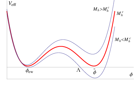
Refer to caption — Figure 1: Schematic representation of the SM effective potential for different values of the Higgs boson mass. For $M_{h}<M_{h}^{c}$ , the electroweak vacuum is unstable.

The absolute stability bound on the Higgs boson mass can be obtained by defining a “critical” mass, $M_{h}^{c}$ , for which the value of the effective potential at the electroweak minimum, $\phi_{\rm{ew}}$ , and at a second minimum, $\tilde{\phi}>\phi_{\rm{ew}}$ , are the same. Analytically, this translates into the three conditions:

		$\displaystyle V_{\rm{eff}}(\phi_{\rm{ew}},M_{h}^{c};\xi)-V_{\rm{eff}}(\tilde{\phi},M_{h}^{c};\xi)=0\,,$		(68)
		$\displaystyle\left.\frac{\partial V_{\rm{eff}}}{\partial\phi}\right\|_{\phi_{\rm{ew}},M_{h}^{c}}=\left.\frac{\partial V_{\rm{eff}}}{\partial\phi}\right\|_{\tilde{\phi},M_{h}^{c}}=0\,.$		(69)

In the $\phi\gg\phi_{\rm{ew}}$ limit, the RG improved SM effective potential is well approximated by

V_{\rm{eff}}(\phi)=\left(\frac{\Omega_{\rm{eff}}(\phi)}{\phi^{4}}-\frac{1}{2}\frac{m_{\rm{eff}}^{2}(\phi)}{\phi^{2}}+\frac{1}{4}\lambda_{\rm{eff}}(\phi)\right)\phi^{4}\approx\frac{1}{4}\lambda_{\rm{eff}}(\phi)\phi^{4}\,.

(70)

Indeed, at the leading order in the $m^{2}/\phi^{2}$ expansion, where $m^{2}\sim\phi_{\rm{ew}}^{2}$ is the electroweak parameter of the Higgs potential, the effective couplings $\Omega_{\rm{eff}}$ and $m^{2}_{\rm{eff}}$ turn out to be proportional to $m^{4}$ and $m^{2}$ respectively.⁶⁶ 6 Moreover, since the beta function of $m$ is proportional to $m$ itself, the value of $m$ does not change much even after a scale running of many orders of magnitude. Hence, the absolute stability condition in Eqs. (68)–(69) can be equivalently rewritten in the following way [5]:

	$\displaystyle\lambda_{\rm{eff}}(\tilde{\phi},M_{h}^{c};\xi)=0\,,$		(71)
	$\displaystyle\left.\frac{\partial\lambda_{\rm{eff}}}{\partial\phi}\right\|_{\tilde{\phi},M_{h}^{c}}=0\,,$		(72)

up to $\phi_{\rm{ew}}^{2}/\tilde{\phi}^{2}\ll 1$ corrections.

On the other hand, due to the explicit presence of $\xi$ in the vacuum stability condition, it is not obvious a priori which are the physical (gauge-independent) observables entering the vacuum stability analysis. The basic tool, in order to capture the gauge-invariant content of the effective potential is given by the Nielsen identity [30]

\frac{\partial}{\partial\xi}V_{\text{eff}}(\phi,\xi)=-C(\phi,\xi)\frac{\partial}{\partial\phi}V_{\text{eff}}(\phi,\xi)\,,

(73)

where $C(\phi,\xi)$ is a correlator involving the ghost fields and the gauge-fixing functional, whose explicit expression will not be needed for our argument. Eq. (73) is valid for the class of linear gauges and can be derived from the BRST non-invariance of a composite operator involving the ghost field and the gauge fixing functional (see e.g. [37] for a concise derivation).

The identity in Eq. (73) carries the following interpretation: the effective potential is gauge independent where it is stationary and hence spontaneous symmetry breaking is a gauge-invariant statement. In the rest of this section we will use the Nielsen identity, in combination with the vacuum stability condition in Eqs. (68)–(69), in order to formally prove that the critical Higgs boson mass, $M_{h}^{c}$ , is a gauge-independent quantity, while the position of the extrema of the effective potential (e.g. $\tilde{\phi}$ ) or the point where $V_{\rm{eff}}$ takes a special value (for instance zero) are essentially gauge dependent.

Our arguments are similar to those presented in Ref. [46], about the gauge independence of the critical temperature of a first order phase transition in the context of the finite temperature effective potential.

3.1 Gauge independence of the critical Higgs boson mass

Let us assume that simultaneously inverting Eqs. (68)–(69) would yield gauge dependent field values and critical Higgs boson mass: $\phi_{\rm{ew}}=\phi_{\rm{ew}}(\xi)$ , $\tilde{\phi}=\tilde{\phi}(\xi)$ and $M_{h}^{c}=M_{h}^{c}(\xi)$ . The total differential of Eq. (68) with respect to $\xi$ then reads

\left.\frac{\partial V_{\rm{eff}}}{\partial\phi}\right|_{\phi_{\rm{ew}},M_{h}^{c}}\frac{\partial\phi_{\rm{ew}}}{\partial\xi}+\left.\frac{\partial V_{\rm{eff}}}{\partial M_{h}}\right|_{\phi_{\rm{ew}},M_{h}^{c}}\frac{\partial M_{h}^{c}}{\partial\xi}+\left.\frac{\partial V_{\rm{eff}}}{\partial\xi}\right|_{\phi_{\rm{ew}},M_{h}^{c}}=\\ \left.\frac{\partial V_{\rm{eff}}}{\partial\phi}\right|_{\tilde{\phi},M_{h}^{c}}\frac{\partial\tilde{\phi}}{\partial\xi}+\left.\frac{\partial V_{\rm{eff}}}{\partial M_{h}}\right|_{\tilde{\phi},M_{h}^{c}}\frac{\partial M_{h}^{c}}{\partial\xi}+\left.\frac{\partial V_{\rm{eff}}}{\partial\xi}\right|_{\tilde{\phi},M_{h}^{c}}\,.

(74)

The first term in both the left-hand side (lhs) and the right-hand side (rhs) of Eq. (74) vanishes because of the stationary conditions in Eq. (69). The third term in both the lhs and the rhs of Eq. (74) vanishes for the same reason, after using the Nielsen identity. Hence, we are left with

\left(\left.\frac{\partial V_{\rm{eff}}}{\partial M_{h}}\right|_{\phi_{\rm{ew}},M_{h}^{c}}-\left.\frac{\partial V_{\rm{eff}}}{\partial M_{h}}\right|_{\tilde{\phi},M_{h}^{c}}\right)\frac{\partial M_{h}^{c}}{\partial\xi}=0\,.

(75)

Since the expression in the bracket of Eq. (75) is in general different from zero, one concludes that

\frac{\partial M_{h}^{c}}{\partial\xi}=0\,,

(76)

namely, the critical Higgs boson mass is gauge independent. Let us notice, however, that the statement above formally holds at all orders in perturbation theory.

3.2 Gauge dependence of the extrema of the effective potential

Let us consider now the total differential with respect to $\xi$ of the second expression in Eq. (69)

\left.\frac{\partial^{2}V_{\rm{eff}}}{\partial\phi^{2}}\right|_{\tilde{\phi},M_{h}^{c}}\frac{\partial\tilde{\phi}}{\partial\xi}+\left.\frac{\partial^{2}V_{\rm{eff}}}{\partial M_{h}\ \partial\phi}\right|_{\tilde{\phi},M_{h}^{c}}\frac{\partial M_{h}^{c}}{\partial\xi}+\left.\frac{\partial^{2}V_{\rm{eff}}}{\partial\xi\ \partial\phi}\right|_{\tilde{\phi},M_{h}^{c}}=0\,.

(77)

The second term is zero due to Eq. (76). By differentiating the Nielsen identity with respect to $\phi$ , and evaluating it at the point $(\tilde{\phi},M_{h}^{c})$ , we get

\left.\frac{\partial^{2}V_{\text{eff}}}{\partial\phi\ \partial\xi}\right|_{\tilde{\phi},M_{h}^{c}}=-\left.\frac{\partial C}{\partial\phi}\right|_{\tilde{\phi},M_{h}^{c}}\left.\frac{\partial V_{\text{eff}}}{\partial\phi}\right|_{\tilde{\phi},M_{h}^{c}}-C(\tilde{\phi},\xi)\left.\frac{\partial^{2}V_{\text{eff}}}{\partial\phi^{2}}\right|_{\tilde{\phi},M_{h}^{c}}\,.

(78)

The first term in the rhs of Eq. (78) vanishes because of the stationary condition in Eq. (69). Hence, we can substitute the third term in Eq. (77), by means of Eq. (78), and get:

\left(\frac{\partial\tilde{\phi}}{\partial\xi}-C(\tilde{\phi},\xi)\right)\left.\frac{\partial^{2}V_{\text{eff}}}{\partial\phi^{2}}\right|_{\tilde{\phi},M_{h}^{c}}=0\,.

(79)

Since the curvature at the extremum is in general different from zero, Eq. (79) implies

\frac{\partial\tilde{\phi}}{\partial\xi}=C(\tilde{\phi},\xi)\,.

(80)

The same holds for any extremum of the effective potential, like e.g. the maximum in Fig. 1 or the electroweak minimum $\phi_{\rm{ew}}$ . This latter fact should not actually come as a surprise. The explicit gauge dependence of the unrenormalized $\phi_{\rm{ew}}$ in the $R_{\xi}$ gauge was discussed for instance in [54] and in the case of the SM it can be found in [55]. A renormalized gauge-invariant $\phi_{\rm{ew}}$ can always be defined by subtracting the divergent and gauge-dependent contributions to $\phi_{\rm{ew}}$ at on-shell points in terms of physical quantities.

3.3 Gauge dependence of the SM vacuum instability scale

The SM vacuum instability scale is operatively defined as the field value $\phi=\Lambda$ , for which the effective potential has the same depth of the electroweak minimum (see e.g. Fig. 1). This is analytically expressed by

V_{\text{eff}}(\Lambda;\xi)=V_{\text{eff}}(\phi_{\rm{ew}};\xi)\,.

(81)

The rhs of Eq. (81) is a gauge-independent quantity, since $\phi_{\rm{ew}}$ is by definition a minimum and we can apply the Nielsen identity. Hence, by solving Eq. (81), one has in general $\Lambda=\Lambda(\xi)$ . In particular, by taking the total differential of Eq. (81) with respect to $\xi$ , we get

\left.\frac{\partial V_{\text{eff}}}{\partial\phi}\right|_{\Lambda}\frac{\partial\Lambda}{\partial\xi}+\left.\frac{\partial V_{\text{eff}}}{\partial\xi}\right|_{\Lambda}=0\,.

(82)

By using the Nielsen identity, we can substitute back the second term in Eq. (82), thus obtaining

\left(\frac{\partial\Lambda}{\partial\xi}-C(\Lambda,\xi)\right)\left.\frac{\partial V_{\text{eff}}}{\partial\phi}\right|_{\Lambda}=0\,.

(83)

Since, in general, $\Lambda$ is not an extremum of the effective potential, Eq. (83) yields

\frac{\partial\Lambda}{\partial\xi}=C(\Lambda,\xi)\,.

(84)

4 Numerical analysis

In this Section we numerically estimate the gauge dependence of the SM vacuum instability scale $\Lambda$ . Let us first focus on the case of the Fermi gauge. Since in the SM $\Lambda\gg\phi_{\rm{ew}}$ , the condition in Eq. (81) is well approximated by (see also Eq. (70))

\lambda_{\rm{eff}}(\Lambda)=0\,,

(85)

up to corrections of ${\cal O}(\phi_{\rm{ew}}^{2}/\Lambda^{2})$ . For the onset of the RG running, we choose $\mu(0)=M_{t}$ (hence $\mu(t)=M_{t}e^{t}$ ), where $M_{t}=173.35\ \rm{GeV}$ is the pole mass of the top quark and we consider the central values of the SM parameters taken from [9]:⁷⁷ 7 Notice that these values are extracted from experimental data with two-loop accuracy. However, we will not perform a NNLO analysis, since the issue of the gauge dependence of the instability scale already arises at the NLO level.

$\displaystyle\lambda(M_{t})$	$\displaystyle=0.12710\,,$	(86)
$\displaystyle y_{t}(M_{t})$	$\displaystyle=0.93697\,,$	(87)
$\displaystyle g_{3}(M_{t})$	$\displaystyle=1.1666\,,$	(88)
$\displaystyle g(M_{t})$	$\displaystyle=0.6483\,,$	(89)
$\displaystyle g^{\prime}(M_{t})$	$\displaystyle=0.3587\,.$	(90)

In order to resum possible large logs in Eq. (67) due to the growth of the anomalous dimension, we make the scale choice

\mu(\overline{t})=e^{\Gamma(\overline{t})}\phi\,,

(91)

which implicitly defines $\overline{t}$ as a function of $\phi$ . Then the effective quartic coupling can be written as

\lambda_{\rm{eff}}(\phi)=e^{4\Gamma(\overline{t}(\phi))}\left[\lambda(\overline{t}(\phi))+\frac{1}{(4\pi)^{2}}\sum_{p}N_{p}\kappa_{p}^{2}(\overline{t}(\phi))\left(\log\kappa_{p}(\overline{t}(\phi))-C_{p}\right)\right]\,.

(92)

Since the overall exponential factor in Eq. (92) never changes the zeros of $\lambda_{\rm{eff}}(\phi)$ , in order to find the instability scale, $\Lambda$ , it is equivalent (and also numerically more convenient) to seek directly the zeros of $\lambda_{\rm{eff}}(\phi)e^{-4\Gamma(\overline{t}(\phi))}$ in terms of the parameter $\overline{t}_{\Lambda}\equiv\overline{t}(\Lambda)$ , defined by⁸⁸ 8 It may actually happen that $\lambda$ turns negative before approaching the instability scale. In such a case, $\log\kappa_{p}$ develops an imaginary part for $p=h,A^{\pm},B^{\pm}$ (see Table 1). Though the imaginary part of the effective potential might have an interpretation in terms of a decay rate of an unstable state [56], the role of such an imaginary component in the determination of the instability scale is not clear. Hence, we pragmatically require only the real part of Eq. (93) to be zero and notice that this problem has nothing to do with the issue of the gauge dependence, since it occurs also in the standard analysis in the Landau gauge.

\lambda(\overline{t}_{\Lambda})+\frac{1}{(4\pi)^{2}}\sum_{p}N_{p}\kappa_{p}^{2}(\overline{t}_{\Lambda})\left(\log\kappa_{p}(\overline{t}_{\Lambda})-C_{p}\right)=0\,,

(93)

and then relate it to the instability scale by inverting Eq. (91)

\Lambda=\mu(\overline{t}_{\Lambda})e^{-\Gamma(\overline{t}_{\Lambda})}=M_{t}e^{\overline{t}_{\Lambda}-\Gamma(\overline{t}_{\Lambda})}\,,

(94)

where we recall the definition (see Eq. (63))

\Gamma(\overline{t}_{\Lambda})=-\int_{0}^{\overline{t}_{\Lambda}}\gamma(t)\,dt\,.

(95)

Before discussing in more detail the gauge dependence of $\Lambda$ , let us turn to the issue of the UV behaviour of the gauge fixing parameters $\xi_{W}$ and $\xi_{B}$ for the Fermi gauge. Their RGEs are collected in Appendix A and can be easily integrated at one loop (see Appendix A.1). While the running of the Abelian gauge-fixing parameter $\xi_{B}$ is very simple ( $\xi_{B}g^{\prime 2}$ is actually constant under the RG flow, as a consequence of a Ward identity) two peculiar RG behaviours can be identified for $\xi_{W}$ . For $\xi_{W}(M_{t})\gg\frac{1}{6}$ one has a quasi-fixed point in the UV (cf. left panel in Fig. 2), while, for $\xi_{W}(M_{t})<0$ , the running can easily generate a Landau pole (cf. right panel in Fig. 2).

The gauge dependence of $\Lambda$ (cf. Eq. (94)) comes both from $t_{\Lambda}$ and $\Gamma(t_{\Lambda})$ . The former is due to the couplings $\kappa_{p}$ , when $p$ runs over $A^{\pm}$ and $B^{\pm}$ (cf. Eq. (93) and Table 1), while the latter is because of the gauge dependence of the anomalous dimension. The running of the anomalous dimension and its integral, $\Gamma$ , are shown in Fig. 3 for three different initial values of $\xi\equiv\xi_{B}(M_{t})=\xi_{W}(M_{t})$ .

From the right panel in Fig. 3 one can see that if $\left|\xi\right|$ is large enough, $\Gamma$ can easily be of $\mathcal{O}(1)$ at intermediate scales below the Planck mass. This justifies the choice of scale done in Eq. (91), which resums the potentially large logs in Eq. (67).

The gauge dependence of the instability scale is shown in Fig. 4. For simplicity, we set $\xi_{W}(M_{t})=\xi_{B}(M_{t})\equiv\xi$ . In addition, we employ two-loop RGEs for all the parameters in Eq. (93) and Eq. (95) that determine $\Lambda$ . The higher-order RGEs allow us to resum the leading and next-to-leading logarithms implicitly contained in Eq. (94). For illustration, we depict with a dashed line in Fig. 4 the gauge dependence of the instability scale obtained without running the gauge-fixing parameters ( $\beta_{\xi}=0$ case). As it can be read from the figure the difference between the resummed (full line) and not resummed one (dashed line) amounts to more than three orders of magnitude. However, even after performing the resummation, the instability scale in the Fermi gauge increases by almost an order of magnitude when the gauge-fixing parameters are varied in the interval $[0,300]$ . Let us also mention that by varying the SM parameters within their experimental uncertainties (e.g. for a lower top mass) the gauge dependence of the scale $\Lambda$ is always found to be of about one order of magnitude.

Another important aspect for the analysis of the gauge dependence of $\Lambda$ is the determination of the perturbativity domain of the gauge fixing parameters $\xi_{W,B}$ . For instance, for the gauge-fixing parameter $\xi_{W}$ one can require that the two-loop correction to its beta function is smaller than the one-loop contribution, thus obtaining (cf. Eq. (105) in Appendix A):

\left|\frac{\xi_{W}^{2}\alpha_{2}^{2}}{(4\pi)^{2}}\right|<\left|\frac{\xi_{W}\alpha_{2}}{4\pi}\right|\,,

(96)

which sets the absolute upper bound

|\xi_{W}|<\frac{4\pi}{\alpha_{2}}\,.

(97)

Taking $\alpha_{2}(M_{t})\approx 0.033$ ,⁹⁹ 9 For $\alpha_{2}(\mu>M_{t})$ the bound becomes less stringent, due to the asymptotic freedom of $\alpha_{2}$ in the SM. one gets $|\xi_{W}(M_{t})|<376$ . Notice, however, that this estimate does not take into account the running of $\xi_{W}$ . For $\xi_{W}(M_{t})\lesssim-5$ a Landau pole can be developed before the Planck scale (cf. right panel in Fig. 2), and perturbation theory starts soon to break down. This is why we do not show the negative branch of the plot in Fig. 4. On the contrary, the running behaviour for $\xi\gg 0$ is smoother, with a quasi-fixed point in the UV for $\xi_{W}$ (cf. left panel in Fig. 2). By studying the evolution of the gauge-dependent anomalous dimension at one, two and three loops we verified, for instance, that $\xi\approx 300$ is still in the perturbative regime. Nonetheless, for a more solid statement about the perturbative domain of $\xi$ , one should inspect the gauge dependent two-loop effective potential, whose calculation goes beyond the scope of the present paper and it is postponed for a future work. One can imagine, however, that a similar condition as in Eq. (96) will be at play, since the gauge-fixing parameters are always associated with the square of the gauge couplings, both in the propagators and in the vertices of the theory.

Finally, for a comprehensive analysis one should also vary the gauge-fixing condition itself. In Appendix B we report on the calculation of the SM one-loop effective potential in a background $R_{\xi}$ gauge. A numerical study, similar to the one presented in this Section, shows that the instability scale decreases by another order of magnitude when the gauge-fixing parameters are varied in their perturbative domain. Such a qualitatively different behaviour in the background $R_{\xi}$ gauge can be understood by noticing the sign flip (with respect to the case of the Fermi gauge) in the contribution of the gauge-fixing parameters to the one-loop anomalous dimension of $\phi$ in Eq. (107). We can thus conclude that the gauge dependence of the instability scale materializes in a variation of about two orders of magnitude, depending on the choice of the gauge condition and of the gauge-fixing parameters. This strengthens our statement that the instability scale $\Lambda$ as defined in Eq. (85) should not be interpreted as a physical quantity.

5 Discussion and conclusions

Once a calculable UV completion of the SM is specified (for instance, the SM itself extrapolated at extremely high energies¹⁰¹⁰ 10 Under the assumption that Planck-scale physics decouples from the SM even at energies beyond the Planck mass and that the Laundau pole of the hypercharge does not pose any conceptual problem.) the fate of the electroweak vacuum, whether it is absolutely stable or not, is a physical statement which does not depend on the choice of the gauge. This is equivalent to say that the critical Higgs boson mass (or, in general, the critical values of the SM parameters) distinguishing between the stable and unstable phase of the SM is a gauge-independent quantity, as we formally proved in Sect. 3.1. In this respect, it is worth to recall that the tunnelling probability of the electroweak vacuum is formally gauge independent as well [57, 37, 21].

On the other hand, the absolute stability condition is sometimes formulated by requiring that the electroweak minimum, $\phi_{\rm{ew}}$ , is the global minimum of the effective potential over the range of validity of the SM

V_{\rm{eff}}(\phi_{\rm{ew}})<V_{\rm{eff}}(\phi)\quad\rm{for}\quad\phi<\Lambda_{\rm{SM}}\,,

(98)

where $\Lambda_{\rm{SM}}$ is a physical threshold (e.g. the Planck scale). Above this scale new physics is supposed to alter the shape of the effective potential. However, since $V_{\rm{eff}}(\phi)$ is gauge dependent (unless $\phi$ is an extremum), the condition in Eq. (98) is clearly gauge dependent too.
From a low-energy point of view, it is a relevant question to seek a connection between the instability scale, $\Lambda$ , and the scale of new physics, $\Lambda_{\rm{SM}}$ . The latter being, of course, of utmost importance for experiments. The irreducible gauge dependence of $\Lambda$ , however, makes its identification with $\Lambda_{\rm{SM}}$ ambiguous, since we are not comparing two physical quantities.

Though the gauge dependence of $\Lambda$ amounts to about one order of magnitude in the case of the Fermi gauge (cf. Fig. 4), this result cannot be used to give an absolute upper bound on the gauge dependence of $\Lambda$ . The reason is that, on one hand, different gauge-fixing schemes generally lead to different results (as, for instance, in the case of the background $R_{\xi}$ gauge discussed in Appendix B) and, on the other hand, we cannot say much beyond perturbation theory. Notice, indeed, that there is no physical principle that restricts the range of the gauge-fixing parameters. Hence, we rather stick to the conclusion that $\Lambda_{\rm{SM}}$ is a model dependent parameter which cannot be determined by just extrapolating the SM parameters at high energies.¹¹¹¹ 11 Even without considering the issue of the gauge dependence, the connection between $\Lambda$ and the maximum allowed value of the scale of new physics required to stabilize the electroweak vacuum is anyway not so direct, due to the presence of extra parameters (e.g. couplings and masses) in any UV completion of the SM [58, 59].

Let us finally recall that, given the central values of the SM parameters and assuming that new physics at e.g. the Planck scale does not affect the tunnelling computation [11], the lifetime of the electroweak vacuum turns out to be much longer than the age of the universe [9]. A metastable electroweak vacuum can comply with the data and new physics is not necessarily implied. Hence, the problem of the gauge dependence of the SM vacuum instability scale and its connection with the scale of new physics might seem an academic one. However, this does not need to be necessarily the case. For instance, we would like to mention the recent measurement of the primordial tensor fluctuations in the cosmic microwave background by the BICEP2 collaboration [60] which suggests a high inflationary scale of about $10^{14}$ GeV. As pointed out in [61, 62, 63, 64, 65, 66] the Higgs field might be subject to quantum fluctuations generated during the primordial stage of inflation which can easily destabilize the electroweak vacuum. In particular, since the quantity $\Lambda$ (or, more precisely, the field value where the effective potential reaches its maximum) enters in the calculation of the electroweak vacuum survival probability, its physical identification should be addressed with care.

Acknowledgments

We thank Stefano Bertolini, Ramona Gröber and Marco Nardecchia for useful discussions. This work was supported by the DFG through the SFB/TR 9 “Computational Particle Physic”.

Appendix A Renormalization group equations

In terms of the parameters $\alpha_{1}=\frac{5}{3}\frac{g^{\prime 2}}{4\pi}$ , $\alpha_{2}=\frac{g^{2}}{4\pi}$ , $\alpha_{3}=\frac{g_{3}^{2}}{4\pi}$ , $\alpha_{t}=\frac{y_{t}^{2}}{4\pi}$ and $\alpha_{\lambda}=\frac{\lambda}{4\pi}$ , the two-loop RGEs used in the numerical analysis for the case of the Fermi gauge are [51, 67, 68, 69]

$\displaystyle\mu^{2}\frac{d}{d\mu^{2}}\frac{\alpha_{1}}{\pi}$	$\displaystyle=\frac{41}{40}\frac{\alpha_{1}^{2}}{\pi^{2}}+\frac{199}{800}\frac{\alpha_{1}^{3}}{\pi^{3}}+\frac{27}{160}\frac{\alpha_{1}^{2}}{\pi^{2}}\frac{\alpha_{2}}{\pi}+\frac{11}{20}\frac{\alpha_{1}^{2}}{\pi^{2}}\frac{\alpha_{3}}{\pi}-\frac{17}{160}\frac{\alpha_{1}^{2}}{\pi^{2}}\frac{\alpha_{t}}{\pi}\,,$	(99)
$\displaystyle\mu^{2}\frac{d}{d\mu^{2}}\frac{\alpha_{2}}{\pi}$	$\displaystyle=-\frac{19}{24}\frac{\alpha_{2}^{2}}{\pi^{2}}+\frac{9}{160}\frac{\alpha_{1}}{\pi}\frac{\alpha_{2}^{2}}{\pi^{2}}+\frac{35}{96}\frac{\alpha_{2}^{3}}{\pi^{3}}+\frac{3}{4}\frac{\alpha_{2}^{2}}{\pi^{2}}\frac{\alpha_{3}}{\pi}-\frac{3}{32}\frac{\alpha_{2}^{2}}{\pi^{2}}\frac{\alpha_{t}}{\pi}\,,$	(100)
$\displaystyle\mu^{2}\frac{d}{d\mu^{2}}\frac{\alpha_{3}}{\pi}$	$\displaystyle=-\frac{7}{4}\frac{\alpha_{3}^{2}}{\pi^{2}}+\frac{11}{160}\frac{\alpha_{1}}{\pi}\frac{\alpha_{3}^{2}}{\pi^{2}}+\frac{9}{32}\frac{\alpha_{2}}{\pi}\frac{\alpha_{3}^{2}}{\pi^{2}}-\frac{13}{8}\frac{\alpha_{3}^{3}}{\pi^{3}}-\frac{1}{8}\frac{\alpha_{3}^{2}}{\pi^{2}}\frac{\alpha_{t}}{\pi}\,,$	(101)
$\displaystyle\mu^{2}\frac{d}{d\mu^{2}}\frac{\alpha_{t}}{\pi}$	$\displaystyle=\frac{\alpha_{t}}{\pi}\left(\frac{9}{8}\frac{\alpha_{t}}{\pi}-\frac{17}{80}\frac{\alpha_{1}}{\pi}-\frac{9}{16}\frac{\alpha_{2}}{\pi}-2\frac{\alpha_{3}}{\pi}\right)+\frac{\alpha_{t}}{\pi}\left(\frac{3}{8}\frac{\alpha_{\lambda}^{2}}{\pi^{2}}-\frac{3}{4}\frac{\alpha_{\lambda}}{\pi}\frac{\alpha_{t}}{\pi}-\frac{3}{4}\frac{\alpha_{t}^{2}}{\pi^{2}}+\frac{393}{1280}\frac{\alpha_{1}}{\pi}\frac{\alpha_{t}}{\pi}\right.$
	$\displaystyle\left.+\frac{225}{256}\frac{\alpha_{2}}{\pi}\frac{\alpha_{t}}{\pi}+\frac{9}{4}\frac{\alpha_{3}}{\pi}\frac{\alpha_{t}}{\pi}+\frac{1187}{9600}\frac{\alpha_{1}^{2}}{\pi^{2}}-\frac{23}{64}\frac{\alpha_{2}^{2}}{\pi^{2}}-\frac{27}{4}\frac{\alpha_{3}^{2}}{\pi^{2}}-\frac{9}{320}\frac{\alpha_{1}}{\pi}\frac{\alpha_{2}}{\pi}+\frac{19}{240}\frac{\alpha_{1}}{\pi}\frac{\alpha_{3}}{\pi}\right.$
	$\displaystyle\left.+\frac{9}{16}\frac{\alpha_{2}}{\pi}\frac{\alpha_{3}}{\pi}\right)\,,$	(102)
$\displaystyle\mu^{2}\frac{d}{d\mu^{2}}\frac{\alpha_{\lambda}}{\pi}$	$\displaystyle=\frac{27}{1600}\frac{\alpha_{1}^{2}}{\pi^{2}}+\frac{9}{160}\frac{\alpha_{1}}{\pi}\frac{\alpha_{2}}{\pi}+\frac{9}{64}\frac{\alpha_{2}^{2}}{\pi^{2}}-\frac{3}{4}\frac{\alpha_{t}^{2}}{\pi^{2}}+\frac{\alpha_{\lambda}}{\pi}\left(-\frac{9}{40}\frac{\alpha_{1}}{\pi}-\frac{9}{8}\frac{\alpha_{2}}{\pi}+\frac{3}{2}\frac{\alpha_{t}}{\pi}+3\frac{\alpha_{\lambda}}{\pi}\right)$	(103)
	$\displaystyle-\frac{3411}{64000}\frac{\alpha_{1}^{3}}{\pi^{3}}-\frac{1677}{12800}\frac{\alpha_{1}^{2}}{\pi^{2}}\frac{\alpha_{2}}{\pi}-\frac{171}{3200}\frac{\alpha_{1}^{2}}{\pi^{2}}\frac{\alpha_{t}}{\pi}+\frac{1887}{6400}\frac{\alpha_{1}^{2}}{\pi^{2}}\frac{\alpha_{\lambda}}{\pi}-\frac{289}{2560}\frac{\alpha_{1}}{\pi}\frac{\alpha_{2}^{2}}{\pi^{2}}+\frac{63}{320}\frac{\alpha_{1}}{\pi}\frac{\alpha_{2}}{\pi}\frac{\alpha_{t}}{\pi}$
	$\displaystyle+\frac{117}{640}\frac{\alpha_{1}}{\pi}\frac{\alpha_{2}}{\pi}\frac{\alpha_{\lambda}}{\pi}-\frac{1}{20}\frac{\alpha_{1}}{\pi}\frac{\alpha_{t}^{2}}{\pi^{2}}+\frac{17}{64}\frac{\alpha_{1}}{\pi}\frac{\alpha_{t}}{\pi}\frac{\alpha_{\lambda}}{\pi}+\frac{27}{40}\frac{\alpha_{1}}{\pi}\frac{\alpha_{\lambda}^{2}}{\pi^{2}}+\frac{305}{512}\frac{\alpha_{2}^{3}}{\pi^{3}}-\frac{9}{128}\frac{\alpha_{2}^{2}}{\pi^{2}}\frac{\alpha_{t}}{\pi}-\frac{73}{256}\frac{\alpha_{2}^{2}}{\pi^{2}}\frac{\alpha_{\lambda}}{\pi}$
	$\displaystyle+\frac{45}{64}\frac{\alpha_{2}}{\pi}\frac{\alpha_{t}}{\pi}\frac{\alpha_{\lambda}}{\pi}+\frac{27}{8}\frac{\alpha_{2}}{\pi}\frac{\alpha_{\lambda}^{2}}{\pi}-\frac{\alpha_{3}}{\pi}\frac{\alpha_{t}^{2}}{\pi^{2}}+\frac{5}{2}\frac{\alpha_{3}}{\pi}\frac{\alpha_{t}}{\pi}\frac{\alpha_{\lambda}}{\pi}+\frac{15}{16}\frac{\alpha_{t}^{3}}{\pi^{3}}-\frac{3}{32}\frac{\alpha_{t}^{2}}{\pi}\frac{\alpha_{\lambda}}{\pi}-\frac{9}{2}\frac{\alpha_{t}}{\pi}\frac{\alpha_{\lambda}^{2}}{\pi^{2}}-\frac{39}{4}\frac{\alpha_{\lambda}^{3}}{\pi^{3}}\,,$
$\displaystyle\mu^{2}\frac{d}{d\mu^{2}}\frac{\xi_{B}}{\pi}$	$\displaystyle=\frac{\xi_{B}}{\pi}\left(-\frac{41}{40}\frac{\alpha_{1}}{\pi}\right)+\frac{\xi_{B}}{\pi}\left(-\frac{199}{800}\frac{\alpha_{1}^{2}}{\pi^{2}}-\frac{27}{160}\frac{\alpha_{1}}{\pi}\frac{\alpha_{2}}{\pi}-\frac{11}{20}\frac{\alpha_{1}}{\pi}\frac{\alpha_{3}}{\pi}+\frac{17}{160}\frac{\alpha_{1}}{\pi}\frac{\alpha_{t}}{\pi}\right)\,,$	(104)
$\displaystyle\mu^{2}\frac{d}{d\mu^{2}}\frac{\xi_{W}}{\pi}$	$\displaystyle=\frac{\xi_{W}}{\pi}\left(\frac{1}{24}\frac{\alpha_{2}}{\pi}-\frac{1}{4}\frac{\xi_{W}\alpha_{2}}{\pi}\right)$
	$\displaystyle+\frac{\xi_{W}}{\pi}\left(-\frac{9}{160}\frac{\alpha_{1}}{\pi}\frac{\alpha_{2}}{\pi}-\frac{43}{64}\frac{\alpha_{2}^{2}}{\pi^{2}}-\frac{3}{4}\frac{\alpha_{2}}{\pi}\frac{\alpha_{3}}{\pi}+\frac{3}{32}\frac{\alpha_{2}}{\pi}\frac{\alpha_{t}}{\pi}-\frac{11}{32}\frac{\alpha_{2}}{\pi}\frac{\xi_{W}\alpha_{2}}{\pi}-\frac{1}{16}\frac{\xi_{W}^{2}\alpha_{2}^{2}}{\pi^{2}}\right)\,,$	(105)
$\displaystyle\mu\frac{d}{d\mu}\phi$	$\displaystyle=-\phi\left(-\frac{9}{80}\frac{\alpha_{1}}{\pi}-\frac{9}{16}\frac{\alpha_{2}}{\pi}+\frac{3}{4}\frac{\alpha_{t}}{\pi}+\frac{3}{80}\frac{\xi_{B}\alpha_{1}}{\pi}+\frac{3}{16}\frac{\xi_{W}\alpha_{2}}{\pi}\right)$
	$\displaystyle-\phi\left(\frac{3}{8}\frac{\alpha_{\lambda}^{2}}{\pi^{2}}+\frac{1293}{12800}\frac{\alpha_{1}^{2}}{\pi^{2}}+\frac{27}{1280}\frac{\alpha_{2}}{\pi}\frac{\alpha_{1}}{\pi}-\frac{271}{512}\frac{\alpha_{2}^{2}}{\pi^{2}}+\frac{17}{128}\frac{\alpha_{1}}{\pi}\frac{\alpha_{t}}{\pi}-\frac{27}{64}\frac{\alpha_{t}^{2}}{\pi^{2}}+\frac{45}{128}\frac{\alpha_{2}}{\pi}\frac{\alpha_{t}}{\pi}\right.$
	$\displaystyle\left.+\frac{5}{4}\frac{\alpha_{3}}{\pi}\frac{\alpha_{t}}{\pi}+\frac{3}{16}\frac{\xi_{W}\alpha_{2}^{2}}{\pi^{2}}+\frac{3}{128}\frac{\xi_{W}^{2}\alpha_{2}^{2}}{\pi^{2}}\right)\,.$	(106)

In the case of the background $R_{\xi}$ gauge (see Appendix B), the one-loop running of the field $\phi$ is found to be

\mu\frac{d}{d\mu}\phi=-\phi\left(-\frac{9}{80}\frac{\alpha_{1}}{\pi}-\frac{9}{16}\frac{\alpha_{2}}{\pi}+\frac{3}{4}\frac{\alpha_{t}}{\pi}-\frac{3}{80}\frac{\overline{\xi}_{B}\alpha_{1}}{\pi}-\frac{3}{16}\frac{\overline{\xi}_{W}\alpha_{2}}{\pi}\right)\,.

(107)

Notice that, by perturbatively expanding the RGE satisfied by the effective potential in Eq. (57) at the first non-trivial order, the gauge-dependent parts of the one-loop anomalous dimension can be extracted from the $\mu$ -dependent terms of $V^{(1)}_{\rm{eff}}$ , which provides a non-trivial check of the calculation.

A.1 On the UV behaviour of $\xi_{B}$ and $\xi_{W}$

To better understand the running properties of $\xi_{B}$ and $\xi_{W}$ , it turns out to be useful to solve analytically Eqs. (99)–(100) and Eqs. (104)–(105). At one loop we have

$\displaystyle\alpha_{1}(\mu)$	$\displaystyle=\frac{\alpha_{1}(M_{t})}{1-\frac{41}{20}\frac{\alpha_{1}(M_{t})}{\pi}\log\frac{\mu}{M_{t}}}\,,$	(108)
$\displaystyle\alpha_{2}(\mu)$	$\displaystyle=\frac{\alpha_{2}(M_{t})}{1+\frac{19}{12}\frac{\alpha_{2}(M_{t})}{\pi}\log\frac{\mu}{M_{t}}}\,,$	(109)
$\displaystyle\xi_{B}(\mu)$	$\displaystyle=\xi_{B}(M_{t})\left(1-\frac{41}{20}\frac{\alpha_{1}(M_{t})}{\pi}\log\frac{\mu}{M_{t}}\right)\,,$	(110)
$\displaystyle\xi_{W}(\mu)$	$\displaystyle=\frac{\frac{\xi_{W}(M_{t})}{1-6\xi_{W}(M_{t})}\left(1+\frac{19}{12}\frac{\alpha_{2}(M_{t})}{\pi}\log\frac{\mu}{M_{t}}\right)^{\tfrac{1}{19}}}{1+6\frac{\xi_{W}(M_{t})}{1-6\xi_{W}(M_{t})}\left(1+\frac{19}{12}\frac{\alpha_{2}(M_{t})}{\pi}\log\frac{\mu}{M_{t}}\right)^{\tfrac{1}{19}}}\,.$	(111)

The main features of the system of equations above can be summarized as follows:

•

From Eq. (99) and Eq. (104) (or, equivalently, from Eq. (108) and Eq. (110)) it follows that $\alpha_{1}\xi_{B}$ is constant under the RG flow. This property is true at all orders in perturbation theory and is a consequence of the Ward identity $Z^{B}_{3}Z_{\alpha_{1}}=1$ , where $Z^{B}_{3}$ and $Z_{\alpha_{1}}$ are respectively the hypercharge wavefunction and vertex renormalization constants.
•

The values $\xi_{B}=0$ and $\xi_{W}=0$ are fixed points of the RG flow. This property is true at all orders in perturbation theory and guarantees that in the Landau gauge $\xi_{B}\neq 0$ and $\xi_{W}\neq 0$ are not radiatively generated.
•

The value $\xi_{W}=\frac{1}{6}$ is a fixed point of the RG flow at one loop (cf. Eq. (105)). However, such a property does not hold anymore at higher orders.

•

For $\xi_{W}(M_{t})\gg\frac{1}{6}$ and $\mu\gg M_{t}$ , Eq. (111) reaches the asymptotic value

\xi_{W}(\mu)\approx\frac{-\frac{1}{6}\left(1+\frac{19}{12}\frac{\alpha_{2}(M_{t})}{\pi}\log\frac{\mu}{M_{t}}\right)^{\tfrac{1}{19}}}{1-\left(1+\frac{19}{12}\frac{\alpha_{2}(M_{t})}{\pi}\log\frac{\mu}{M_{t}}\right)^{\tfrac{1}{19}}}\,,

(112)

which is independent from the initial condition $\xi_{W}(M_{t})$ and always $>0$ . A typical RG solution in such a case is plotted in the left panel of Fig. 2.

•

For $\xi_{W}(M_{t})<0$ , Eq. (111) can develop a Landau pole. See e.g. the right panel in Fig. 2.

Appendix B Background $R_{\xi}$ gauge

In this appendix we consider the calculation of the SM one-loop effective potential in a generalization of the renormalizable ’t Hooft gauge (see e.g. [70]) where the Higgs vacuum expectation value (vev) is promoted to the background field $\phi$ . This is obtained by considering the following Lagrangian density

\mathcal{L}^{\rm{BKGD}}_{\rm{g.f.}}=-\frac{1}{2}\left[2\bar{F}^{+}\bar{F}^{-}+\left(\bar{F}^{3}\right)^{2}+\left(\bar{F}^{B}\right)^{2}\right]\,,

(113)

where the gauge-fixing functionals are defined as

$\displaystyle\bar{F}^{\pm}$	$\displaystyle=\bar{\xi}_{1,W}^{-1/2}\partial^{\mu}W^{\pm}_{\mu}\mp i\bar{\xi}_{2,W}^{1/2}\bar{m}_{W}\chi^{\pm}\,,$	(114)
$\displaystyle\bar{F}^{3}$	$\displaystyle=\bar{\xi}_{1,3}^{-1/2}\partial^{\mu}W^{3}_{\mu}-\bar{\xi}_{2,3}^{1/2}\bar{m}_{W}\chi^{3}\,,$	(115)
$\displaystyle\bar{F}^{B}$	$\displaystyle=\bar{\xi}_{1,B}^{-1/2}\partial^{\mu}B_{\mu}-\bar{\xi}_{2,B}^{1/2}\bar{m}_{B}\chi^{3}\,,$	(116)

with $W^{\pm}_{\mu}$ and $\chi^{\pm}$ conforming to the standard definitions

	$\displaystyle W^{\pm}_{\mu}$	$\displaystyle=\tfrac{1}{\sqrt{2}}\left(W^{1}_{\mu}\mp iW^{2}_{\mu}\right)\,,$		(117)
	$\displaystyle\chi^{\pm}$	$\displaystyle=\tfrac{1}{\sqrt{2}}\left(\chi^{1}\pm i\chi^{2}\right)\,.$		(118)

In Eqs. (114)–(116), $\bar{m}_{W}$ and $\bar{m}_{B}$ are background-field-dependent masses (see Eqs. (18)–(19)) and the gauge-fixing parameters $\bar{\xi}_{1,\alpha},\bar{\xi}_{2,\alpha}$ (for $\alpha=W,3,B$ ) are denoted differently, since they have a different renormalization constant already at one loop [70].

As long as we are not interested in the running properties of $\bar{\xi}_{1,\alpha}$ and $\bar{\xi}_{2,\alpha}$ , they can be chosen equal at a given renormalization scale. This simplifies the calculation of the one-loop effective potential, since the mixed Goldstone–gauge boson propagators do not appear at tree level. In a first step, we set for simplicity $\bar{\xi}_{1,W}=\bar{\xi}_{2,W}=\bar{\xi}_{1,3}=\bar{\xi}_{2,3}\equiv\bar{\xi}_{W}$ and $\bar{\xi}_{1,B}=\bar{\xi}_{2,B}\equiv\bar{\xi}_{B}$ . For the full result with general gauge-fixing parameters we refer to Appendix B.1.¹²¹² 12 We are aware of a similar calculation in the background $R_{\xi}$ gauge where all the gauge-fixing parameters in Eqs. (114)–(116) are taken equal [46].

A new feature, with respect to the Fermi gauge, is the non-trivial contribution of the ghost fields, which must be taken into account by means of the compensating ghost Lagrangian associated to the gauge-fixing functionals in Eqs. (114)–(115)

\mathcal{L}_{\rm{ghost}}^{\rm{BKGD}}=\sum_{\alpha\beta}c^{\dagger}_{\alpha}\frac{\delta\bar{F}^{\alpha}}{\delta\theta^{\beta}}c_{\beta}\,,

(119)

where $c_{\alpha}$ , $c^{\dagger}_{\alpha}$ ( $\alpha=+,-,3,B)$ are the Feddeev-Popov ghost fields and $\delta/\delta\theta^{\beta}$ denotes the derivative with respect to the parameter of the gauge transformation. Following the definition of the covariant derivative in Eq. (5), the quadratic part of the ghost Lagrangian is found to be

$\displaystyle\mathcal{L}_{\rm{ghost}}^{\rm{BKGD/quad}}$	$\displaystyle=c_{+}^{\dagger}\left(-\bar{\xi}_{W}^{-1/2}\Box-\bar{\xi}_{W}^{1/2}\bar{m}_{W}^{2}\right)c_{+}+c_{-}^{\dagger}\left(-\bar{\xi}_{W}^{-1/2}\Box-\bar{\xi}_{W}^{1/2}\bar{m}_{W}^{2}\right)c_{-}$
	$\displaystyle+c_{3}^{\dagger}\left(-\bar{\xi}_{W}^{-1/2}\Box-\bar{\xi}_{W}^{1/2}\bar{m}_{W}^{2}\right)c_{3}+c_{B}^{\dagger}\left(-\bar{\xi}_{B}^{-1/2}\Box-\bar{\xi}_{B}^{1/2}\bar{m}_{B}^{2}\right)c_{B}$
	$\displaystyle+c_{3}^{\dagger}\left(-\bar{\xi}_{W}^{1/2}\bar{m}_{W}\bar{m}_{B}\right)c_{B}+c_{B}^{\dagger}\left(-\bar{\xi}_{B}^{1/2}\bar{m}_{W}\bar{m}_{B}\right)c_{3}\,.$	(120)

Correspondingly, the inverse propagator matrix of the ghost fields in momentum space is given by

i\tilde{\mathcal{D}}^{-1}_{\rm{ghost}}=\left(\begin{array}[]{cccc}\bar{\xi}_{W}^{-1/2}k^{2}-\bar{\xi}_{W}^{1/2}\bar{m}_{W}^{2}&0&0&0\\ 0&\bar{\xi}_{W}^{-1/2}k^{2}-\bar{\xi}_{W}^{1/2}\bar{m}_{W}^{2}&0&0\\ 0&0&\bar{\xi}_{W}^{-1/2}k^{2}-\bar{\xi}_{W}^{1/2}\bar{m}_{W}^{2}&-\bar{\xi}_{W}^{1/2}\bar{m}_{W}\bar{m}_{B}\\ 0&0&-\bar{\xi}_{B}^{1/2}\bar{m}_{W}\bar{m}_{B}&\bar{\xi}_{B}^{-1/2}k^{2}-\bar{\xi}_{B}^{1/2}\bar{m}_{B}^{2}\end{array}\right)\,,

(121)

defined on the complex field vector basis, $c^{T}=\left(c_{+},c_{-},c_{3},c_{B}\right)$ . Then from Eq. (121) one gets

\log\mbox{det}\,i\tilde{\mathcal{D}}^{-1}_{\rm{ghost}}=2\log\left(k^{2}-\bar{\xi}_{W}\bar{m}_{W}^{2}\right)+\log\left(k^{2}-\bar{\xi}_{W}\bar{m}_{W}^{2}-\bar{\xi}_{B}\bar{m}_{B}^{2}\right)+\ldots\,,

(122)

where the ellipses stand for $\phi$ -independent terms. The rest of the calculation proceeds as in Sect. 2.1, with only two differences: the absence of the Goldstone–gauge boson mixing term, $\bar{m}_{\text{mix}}$ , and the presence of an extra, gauge-dependent, contribution to the Goldstone boson masses

i\tilde{\mathcal{D}}^{-1}_{\chi}=\left(\begin{array}[]{ccc}k^{2}-\bar{m}_{\chi}^{2}-\bar{\xi}_{W}\bar{m}_{W}^{2}&0&0\\ 0&k^{2}-\bar{m}_{\chi}^{2}-\bar{\xi}_{W}\bar{m}_{W}^{2}&0\\ 0&0&k^{2}-\bar{m}_{\chi}^{2}-\bar{\xi}_{W}\bar{m}_{W}^{2}-\bar{\xi}_{B}\bar{m}_{B}^{2}\end{array}\right)\,.

(123)

Including all the relevant degrees of freedom, the one-loop effective potential is given by (cf. Eq. (9))

$\displaystyle V^{(1)}_{\rm{eff}}(\phi)\|^{\rm{BKGD}}$	$\displaystyle=-\frac{i}{2}\mu^{2\epsilon}\int\frac{d^{d}k}{(2\pi)^{d}}\left[-12\log\left(-k^{2}+\bar{m}_{t}^{2}\right)+(d-1)\left(2\log\left(-k^{2}+\bar{m}_{W}^{2}\right)\right.\right.$
	$\displaystyle\left.+\log\left(-k^{2}+\bar{m}_{Z}^{2}\right)\right)+\log\left(k^{2}-\bar{m}_{h}^{2}\right)+2\log\left(k^{2}-\bar{m}_{\chi^{+}}^{2}\right)+\log\left(k^{2}-\bar{m}_{\chi^{0}}^{2}\right)$
	$\displaystyle\left.-2\log\left(k^{2}-\bar{m}_{c_{W}}^{2}\right)-\log\left(k^{2}-\bar{m}_{c_{Z}}^{2}\right)+\,\text{$\phi$-independent}\right]\,,$	(124)

where we defined the field-dependent masses:

$\displaystyle\bar{m}_{c_{W}}^{2}$	$\displaystyle=\bar{\xi}_{W}\bar{m}_{W}^{2}\,,$	(125)
$\displaystyle\bar{m}_{c_{Z}}^{2}$	$\displaystyle=\bar{\xi}_{W}\bar{m}_{W}^{2}+\bar{\xi}_{B}\bar{m}_{B}^{2}\,,$	(126)
$\displaystyle\bar{m}_{\chi^{+}}^{2}$	$\displaystyle=\bar{m}_{\chi}^{2}+\bar{\xi}_{W}\bar{m}_{W}^{2}\,,$	(127)
$\displaystyle\bar{m}_{\chi^{0}}^{2}$	$\displaystyle=\bar{m}_{\chi}^{2}+\bar{\xi}_{W}\bar{m}_{W}^{2}+\bar{\xi}_{B}\bar{m}_{B}^{2}\,.$	(128)

By performing the integral in Eq. (47) and by expanding in $\epsilon$ , we get

		$\displaystyle V^{(1)}_{\rm{eff}}\|_{\rm{bare}}^{\rm{BKGD}}=\frac{1}{4(4\pi)^{2}}\left[-12\bar{m}_{t}^{4}\left(\log\frac{\bar{m}_{t}^{2}}{\mu^{2}}-\frac{3}{2}-\Delta_{\epsilon}\right)+6\bar{m}_{W}^{4}\left(\log\frac{\bar{m}_{W}^{2}}{\mu^{2}}-\frac{5}{6}-\Delta_{\epsilon}\right)\right.$		(129)
		$\displaystyle\left.+3\bar{m}_{Z}^{4}\left(\log\frac{\bar{m}_{Z}^{2}}{\mu^{2}}-\frac{5}{6}-\Delta_{\epsilon}\right)+\bar{m}_{h}^{4}\left(\log\frac{\bar{m}_{h}^{2}}{\mu^{2}}-\frac{3}{2}-\Delta_{\epsilon}\right)+2\bar{m}_{\chi^{+}}^{4}\left(\log\frac{\bar{m}_{\chi^{+}}^{2}}{\mu^{2}}-\frac{3}{2}-\Delta_{\epsilon}\right)\right.$
		$\displaystyle\left.+\bar{m}_{\chi^{0}}^{4}\left(\log\frac{\bar{m}_{\chi^{0}}^{2}}{\mu^{2}}-\frac{3}{2}-\Delta_{\epsilon}\right)-2\bar{m}_{c_{W}}^{4}\left(\log\frac{\bar{m}_{c_{W}}^{2}}{\mu^{2}}-\frac{3}{2}-\Delta_{\epsilon}\right)-\bar{m}_{c_{Z}}^{4}\left(\log\frac{\bar{m}_{c_{Z}}^{2}}{\mu^{2}}-\frac{3}{2}-\Delta_{\epsilon}\right)\right]\,,$

whose divergent part is explicitly given by

	$\displaystyle V^{(1)}_{\rm{eff}}\|_{\rm{bare-pole}}^{\rm{BKGD}}$	$\displaystyle=\frac{\Delta_{\epsilon}}{(4\pi)^{2}}\left[-m^{4}+\left(3\lambda+\frac{1}{8}\bar{\xi}_{B}g^{\prime 2}+\frac{3}{8}\bar{\xi}_{W}g^{2}\right)m^{2}\phi^{2}\right.$
		$\displaystyle\left.+\left(-\frac{3}{64}g^{\prime 4}-\frac{3}{32}g^{\prime 2}g^{2}-\frac{9}{64}g^{4}+\frac{3}{4}y_{t}^{4}-3\lambda^{2}-\frac{1}{8}\bar{\xi}_{B}g^{\prime 2}\lambda-\frac{3}{8}\bar{\xi}_{W}g^{2}\lambda\right)\phi^{4}\right]\,.$		(130)

Notice that the divergent structure of Eq. (130) can be identified with that in Eq. (51) of the Fermi gauge, after the replacement $\overline{\xi}_{W,B}\rightarrow-\xi_{W,B}$ . Hence, in order to cancel the gauge-dependent poles in Eq. (130), the same substitution must be made in the field renormalization constant in Eq. (53), which implies

Z_{\phi}^{1/2}|^{\rm{BKGD}}=1+\frac{\Delta_{\epsilon}}{(4\pi)^{2}}\left(\frac{3}{8}g^{\prime 2}+\frac{9}{8}g^{2}-\frac{3}{2}y_{t}^{2}+\frac{1}{8}\overline{\xi}_{B}g^{\prime 2}+\frac{3}{8}\overline{\xi}_{W}g^{2}\right)\,.\\

(131)

The renormalization constants of $m^{2}$ and $\lambda$ are gauge independent and hence are given by the expressions in Eqs. (54)–(55).

After the subtraction of all the poles due to the renormalization prescription, the one-loop contribution to the effective potential in the $\overline{\rm{MS}}$ scheme reads

$\displaystyle V^{(1)}_{\rm{eff}}(\phi)\|^{\rm{BKGD}}$	$\displaystyle=\frac{1}{4(4\pi)^{2}}\left[-12\bar{m}_{t}^{4}\left(\log\frac{\bar{m}_{t}^{2}}{\mu^{2}}-\frac{3}{2}\right)+6\bar{m}_{W}^{4}\left(\log\frac{\bar{m}_{W}^{2}}{\mu^{2}}-\frac{5}{6}\right)+3\bar{m}_{Z}^{4}\left(\log\frac{\bar{m}_{Z}^{2}}{\mu^{2}}-\frac{5}{6}\right)\right.$
	$\displaystyle\left.+\bar{m}_{h}^{4}\left(\log\frac{\bar{m}_{h}^{2}}{\mu^{2}}-\frac{3}{2}\right)+2\bar{m}_{\chi^{+}}^{4}\left(\log\frac{\bar{m}_{\chi^{+}}^{2}}{\mu^{2}}-\frac{3}{2}\right)+\bar{m}_{\chi^{0}}^{4}\left(\log\frac{\bar{m}_{\chi^{0}}^{2}}{\mu^{2}}-\frac{3}{2}\right)\right.$
	$\displaystyle\left.-2\bar{m}_{c_{W}}^{4}\left(\log\frac{\bar{m}_{c_{W}}^{2}}{\mu^{2}}-\frac{3}{2}\right)-\bar{m}_{c_{Z}}^{4}\left(\log\frac{\bar{m}_{c_{Z}}^{2}}{\mu^{2}}-\frac{3}{2}\right)\right]\,,$	(132)

where the definition of the $\phi$ -dependent mass terms can be found in Eqs. (125)–(128) (see also Eqs. (16)–(20)). For $\overline{\xi}_{W}=\overline{\xi}_{B}=0$ , Eq. (132) reproduces the standard one-loop result in the Landau gauge [24], while, for $\overline{\xi}_{W}=\overline{\xi}_{B}$ , it reproduces the result of [46]. Moreover, on the tree-level minimum, $\bar{m}_{\chi}=0$ , one has $\bar{m}_{\chi^{+}}=\bar{m}_{c_{W}}$ and $\bar{m}_{\chi^{0}}=\bar{m}_{c_{Z}}$ , so that the gauge dependence drops from $V^{(1)}_{\rm{eff}}$ .

By expanding Eq. (132) in the $\phi\gg m$ limit, one gets the RG improved $\lambda_{\rm{eff}}$ coupling defined in Eq. (67), with the $p$ -coefficients explicitly given in Table 2.

$p$	$t$	$W$	$Z$	$h$	$\chi^{+}$	$\chi^{0}$	$c_{W}$	$c_{Z}$
$N_{p}$	$-12$	$6$	$3$	$1$	$2$	$1$	$-2$	$-1$
$C_{p}$	$\frac{3}{2}$	$\frac{5}{6}$	$\frac{5}{6}$	$\frac{3}{2}$	$\frac{3}{2}$	$\frac{3}{2}$	$\frac{3}{2}$	$\frac{3}{2}$
$\kappa_{p}$	$\frac{y_{t}^{2}}{2}$	$\frac{g^{2}}{4}$	$\frac{g^{2}+g^{\prime 2}}{4}$	$3\lambda$	$\lambda+\frac{\bar{\xi}_{W}g^{2}}{4}$	$\lambda+\frac{\bar{\xi}_{B}g^{\prime 2}}{4}+\frac{\bar{\xi}_{W}g^{2}}{4}$	$\frac{\bar{\xi}_{W}g^{2}}{4}$	$\frac{\bar{\xi}_{B}g^{\prime 2}}{4}+\frac{\bar{\xi}_{W}g^{2}}{4}$

Table 2: The

p

-coefficients entering the expression of

\lambda_{\rm{eff}}

in Eq. (67) for the background

R_{\xi}

gauge.

B.1 Full result

The expression of the effective potential in the background $R_{\xi}$ gauge for a general set of gauge-fixing parameters $\bar{\xi}_{1,\alpha},\bar{\xi}_{2,\alpha}$ ( $\alpha=W,3,B$ ) is found to be

$\displaystyle V^{(1)}_{\rm{eff}}\|^{\rm{BKGD}}$	$\displaystyle=\frac{1}{4(4\pi)^{2}}\left[-12\bar{m}_{t}^{4}\left(\log\frac{\bar{m}_{t}^{2}}{\mu^{2}}-\frac{3}{2}\right)+6\bar{m}_{W}^{4}\left(\log\frac{\bar{m}_{W}^{2}}{\mu^{2}}-\frac{5}{6}\right)+3\bar{m}_{Z}^{4}\left(\log\frac{\bar{m}_{Z}^{2}}{\mu^{2}}-\frac{5}{6}\right)\right.$
	$\displaystyle\left.+\bar{m}_{h}^{4}\left(\log\frac{\bar{m}_{h}^{2}}{\mu^{2}}-\frac{3}{2}\right)+2\bar{m}_{A^{+}}^{4}\left(\log\frac{\bar{m}_{A^{+}}^{2}}{\mu^{2}}-\frac{3}{2}\right)+2\bar{m}_{A^{-}}^{4}\left(\log\frac{\bar{m}_{A^{-}}^{2}}{\mu^{2}}-\frac{3}{2}\right)\right.$
	$\displaystyle+\bar{m}_{B^{+}}^{4}\left(\log\frac{\bar{m}_{B^{+}}^{2}}{\mu^{2}}-\frac{3}{2}\right)+\bar{m}_{B^{-}}^{4}\left(\log\frac{\bar{m}_{B^{-}}^{2}}{\mu^{2}}-\frac{3}{2}\right)-4\bar{m}_{c_{W}}^{4}\left(\log\frac{\bar{m}_{c_{W}}^{2}}{\mu^{2}}-\frac{3}{2}\right)$
	$\displaystyle\left.-2\bar{m}_{c_{Z}}^{4}\left(\log\frac{\bar{m}_{c_{Z}}^{2}}{\mu^{2}}-\frac{3}{2}\right)\right]\,,$	(133)

where we employed the $\phi$ -dependent masses in Eqs. (16)–(20) and further defined

$\displaystyle\bar{m}_{A^{\pm}}^{2}$	$\displaystyle=\frac{1}{2}\left(\bar{m}_{\chi}^{2}+2\sqrt{\bar{\xi}_{1,W}\bar{\xi}_{2,W}}\bar{m}_{W}^{2}\pm\bar{m}_{\chi}\sqrt{\bar{m}_{\chi}^{2}-4\left(\bar{\xi}_{1,W}-\sqrt{\bar{\xi}_{1,W}\bar{\xi}_{2,W}}\right)\bar{m}_{W}^{2}}\right)\,,$	(134)
$\displaystyle\bar{m}_{B^{\pm}}^{2}$	$\displaystyle=\frac{1}{2}\left(\bar{m}_{\chi}^{2}+2\sqrt{\bar{\xi}_{1,3}\bar{\xi}_{2,3}}\bar{m}_{W}^{2}+2\sqrt{\bar{\xi}_{1,B}\bar{\xi}_{2,B}}\bar{m}_{B}^{2}\right.$
	$\displaystyle\left.\pm\bar{m}_{\chi}\sqrt{\bar{m}_{\chi}^{2}-4\left(\bar{\xi}_{1,3}-\sqrt{\bar{\xi}_{1,3}\bar{\xi}_{2,3}}\right)\bar{m}_{W}^{2}-4\left(\bar{\xi}_{1,B}-\sqrt{\bar{\xi}_{1,B}\bar{\xi}_{2,B}}\right)\bar{m}_{B}^{2}}\right)\,,$	(135)
$\displaystyle\bar{m}_{c_{W}}^{2}$	$\displaystyle=\sqrt{\bar{\xi}_{1,W}\bar{\xi}_{2,W}}\bar{m}_{W}^{2}\,,$	(136)
$\displaystyle\bar{m}_{c_{Z}}^{2}$	$\displaystyle=\sqrt{\bar{\xi}_{1,3}\bar{\xi}_{2,3}}\bar{m}_{W}^{2}+\sqrt{\bar{\xi}_{1,B}\bar{\xi}_{2,B}}\bar{m}_{B}^{2}\,.$	(137)

While for the gauge-dependent part of the one-loop anomalous dimension we get

\left.\gamma^{(1)}\right|_{\rm{gauge\ dep.}}^{\rm{BKGD}}=\frac{1}{(4\pi)^{2}}\left(\frac{1}{2}\left(\bar{\xi}_{1,W}-2\sqrt{\bar{\xi}_{1,W}\bar{\xi}_{2,W}}\right)g^{2}+\frac{1}{4}\left(\bar{\xi}_{1,3}-2\sqrt{\bar{\xi}_{1,3}\bar{\xi}_{2,3}}\right)g^{2}\right.\\ \left.+\frac{1}{4}\left(\bar{\xi}_{1,B}-2\sqrt{\bar{\xi}_{1,B}\bar{\xi}_{2,B}}\right)g^{\prime 2}\right)\,.

(138)

Notice that in the $\bar{\xi}_{1,\alpha}\rightarrow\bar{\xi}_{2,\alpha}$ limit ( $\alpha=W,3,B$ ) and for $3=W$ one reproduces the background $R_{\xi}$ gauge results in Eq. (132) and Eq. (107), while for $\bar{\xi}_{2,\alpha}\rightarrow 0$ ( $\alpha=W,3,B$ ) and $3=W$ one obtains the expressions in Eq. (56) and Eq. (106) for the Fermi gauge.

Let us finally point out that the SM effective potential in the standard $R_{\xi}$ gauge can be obtained by replacing

\bar{\xi}_{2,\alpha}^{1/2}\rightarrow\bar{\xi}_{2,\alpha}^{1/2}v/\phi\,,

(139)

in the $\phi$ -dependent mass terms of Eq. (133), where $\alpha=W,3,B$ and $v=\sqrt{m^{2}/\lambda}$ denotes the tree-level vev of the Higgs doublet. In the limit relevant for the study of the SM vacuum stability, namely $\phi\gg v$ , the $R_{\xi}$ gauge reduces to the Fermi gauge. On the other hand, the expression of the SM effective potential in the standard $R_{\xi}$ gauge is more suited for broken-phase calculations.

References

[1] ATLAS Collaboration Collaboration, G. Aad et al., “Observation of a new particle in the search for the Standard Model Higgs boson with the ATLAS detector at the LHC,” Phys.Lett. B716 (2012) 1–29, arXiv:1207.7214 [hep-ex].
[2] CMS Collaboration Collaboration, S. Chatrchyan et al., “Observation of a new boson at a mass of 125 GeV with the CMS experiment at the LHC,” Phys.Lett. B716 (2012) 30–61, arXiv:1207.7235 [hep-ex].
[3] M. Holthausen, K. S. Lim, and M. Lindner, “Planck scale Boundary Conditions and the Higgs Mass,” JHEP 1202 (2012) 037, arXiv:1112.2415 [hep-ph].
[4] J. Elias-Miro, J. R. Espinosa, G. F. Giudice, G. Isidori, A. Riotto, et al., “Higgs mass implications on the stability of the electroweak vacuum,” Phys.Lett. B709 (2012) 222–228, arXiv:1112.3022 [hep-ph].
[5] F. Bezrukov, M. Y. Kalmykov, B. A. Kniehl, and M. Shaposhnikov, “Higgs Boson Mass and New Physics,” JHEP 1210 (2012) 140, arXiv:1205.2893 [hep-ph].
[6] G. Degrassi, S. Di Vita, J. Elias-Miro, J. R. Espinosa, G. F. Giudice, et al., “Higgs mass and vacuum stability in the Standard Model at NNLO,” JHEP 1208 (2012) 098, arXiv:1205.6497 [hep-ph].
[7] S. Alekhin, A. Djouadi, and S. Moch, “The top quark and Higgs boson masses and the stability of the electroweak vacuum,” Phys.Lett. B716 (2012) 214–219, arXiv:1207.0980 [hep-ph].
[8] I. Masina, “Higgs boson and top quark masses as tests of electroweak vacuum stability,” Phys.Rev. D87 no. 5, (2013) 053001, arXiv:1209.0393 [hep-ph].
[9] D. Buttazzo, G. Degrassi, P. P. Giardino, G. F. Giudice, F. Sala, et al., “Investigating the near-criticality of the Higgs boson,” JHEP 1312 (2013) 089, arXiv:1307.3536.
[10] O. Antipin, M. Gillioz, J. Krog, E. M¿lgaard, and F. Sannino, “Standard Model Vacuum Stability and Weyl Consistency Conditions,” JHEP 1308 (2013) 034, arXiv:1306.3234.
[11] V. Branchina and E. Messina, “Stability, Higgs Boson Mass and New Physics,” Phys.Rev.Lett. 111 (2013) 241801, arXiv:1307.5193 [hep-ph].
[12] M. Lindner, M. Sher, and H. W. Zaglauer, “Probing Vacuum Stability Bounds at the Fermilab Collider,” Phys.Lett. B228 (1989) 139.
[13] P. B. Arnold, “Can the Electroweak Vacuum Be Unstable?,” Phys.Rev. D40 (1989) 613.
[14] M. Sher, “Electroweak Higgs Potentials and Vacuum Stability,” Phys.Rept. 179 (1989) 273–418.
[15] M. Sher, “Precise vacuum stability bound in the standard model,” Phys.Lett. B317 (1993) 159–163, arXiv:hep-ph/9307342 [hep-ph].
[16] C. Ford, D. Jones, P. Stephenson, and M. Einhorn, “The Effective potential and the renormalization group,” Nucl.Phys. B395 (1993) 17–34, arXiv:hep-lat/9210033 [hep-lat].
[17] G. Altarelli and G. Isidori, “Lower limit on the Higgs mass in the standard model: An Update,” Phys.Lett. B337 (1994) 141–144.
[18] J. Casas, J. Espinosa, and M. Quiros, “Improved Higgs mass stability bound in the standard model and implications for supersymmetry,” Phys.Lett. B342 (1995) 171–179, arXiv:hep-ph/9409458 [hep-ph].
[19] J. Espinosa and M. Quiros, “Improved metastability bounds on the standard model Higgs mass,” Phys.Lett. B353 (1995) 257–266, arXiv:hep-ph/9504241 [hep-ph].
[20] J. Casas, J. Espinosa, and M. Quiros, “Standard model stability bounds for new physics within LHC reach,” Phys.Lett. B382 (1996) 374–382, arXiv:hep-ph/9603227 [hep-ph].
[21] G. Isidori, G. Ridolfi, and A. Strumia, “On the metastability of the standard model vacuum,” Nucl.Phys. B609 (2001) 387–409, arXiv:hep-ph/0104016 [hep-ph].
[22] G. Isidori, V. S. Rychkov, A. Strumia, and N. Tetradis, “Gravitational corrections to standard model vacuum decay,” Phys.Rev. D77 (2008) 025034, arXiv:0712.0242 [hep-ph].
[23] J. Ellis, J. Espinosa, G. Giudice, A. Hoecker, and A. Riotto, “The Probable Fate of the Standard Model,” Phys.Lett. B679 (2009) 369–375, arXiv:0906.0954 [hep-ph].
[24] S. R. Coleman and E. J. Weinberg, “Radiative Corrections as the Origin of Spontaneous Symmetry Breaking,” Phys.Rev. D7 (1973) 1888–1910.
[25] R. Jackiw, “Functional evaluation of the effective potential,” Phys.Rev. D9 (1974) 1686.
[26] L. Dolan and R. Jackiw, “Gauge Invariant Signal for Gauge Symmetry Breaking,” Phys.Rev. D9 (1974) 2904.
[27] J. Kang, “Gauge Invariance of the Scalar-Vector Mass Ratio in the Coleman-Weinberg Model,” Phys.Rev. D10 (1974) 3455.
[28] W. Fischler and R. Brout, “Gauge Invariance in Spontaneously Broken Symmetry,” Phys.Rev. D11 (1975) 905.
[29] J.-M. Frere and P. Nicoletopoulos, “Gauge Invariant Content of the Effective Potential,” Phys.Rev. D11 (1975) 2332.
[30] N. Nielsen, “On the Gauge Dependence of Spontaneous Symmetry Breaking in Gauge Theories,” Nucl.Phys. B101 (1975) 173.
[31] R. Fukuda and T. Kugo, “Gauge Invariance in the Effective Action and Potential,” Phys.Rev. D13 (1976) 3469.
[32] I. Aitchison and C. Fraser, “Gauge Invariance and the Effective Potential,” Annals Phys. 156 (1984) 1.
[33] D. Johnston, “Nielsen Identities in the ’t Hooft Gauge,” Nucl.Phys. B253 (1985) 687.
[34] G. Thompson and H.-L. Yu, “Gauge covariance of the effective potential,” Phys.Rev. D31 (1985) 2141–2144.
[35] R. Kobes, G. Kunstatter, and A. Rebhan, “Gauge dependence identities and their application at finite temperature,” Nucl.Phys. B355 (1991) 1–37.
[36] S. Ramaswamy, “Gauge invariance and the effective potential: The Abelian Higgs model,” Nucl.Phys. B453 (1995) 240–258.
[37] D. Metaxas and E. J. Weinberg, “Gauge independence of the bubble nucleation rate in theories with radiative symmetry breaking,” Phys.Rev. D53 (1996) 836–843, arXiv:hep-ph/9507381 [hep-ph].
[38] O. M. Del Cima, D. H. Franco, and O. Piguet, “Gauge independence of the effective potential revisited,” Nucl.Phys. B551 (1999) 813–825, arXiv:hep-th/9902084 [hep-th].
[39] P. Gambino and P. A. Grassi, “The Nielsen identities of the SM and the definition of mass,” Phys.Rev. D62 (2000) 076002, arXiv:hep-ph/9907254 [hep-ph].
[40] L. P. Alexander and A. Pilaftsis, “The One-Loop Effective Potential in Non-Linear Gauges,” J.Phys. G36 (2009) 045006, arXiv:0809.1580 [hep-ph].
[41] W. Loinaz and R. Willey, “Gauge dependence of lower bounds on the Higgs mass derived from electroweak vacuum stability constraints,” Phys.Rev. D56 (1997) 7416–7426, arXiv:hep-ph/9702321 [hep-ph].
[42] M. Gonderinger, H. Lim, and M. J. Ramsey-Musolf, “Complex Scalar Singlet Dark Matter: Vacuum Stability and Phenomenology,” Phys.Rev. D86 (2012) 043511, arXiv:1202.1316 [hep-ph].
[43] C. Ford, I. Jack, and D. Jones, “The Standard model effective potential at two loops,” Nucl.Phys. B387 (1992) 373–390, arXiv:hep-ph/0111190 [hep-ph].
[44] S. P. Martin, “Two loop effective potential for a general renormalizable theory and softly broken supersymmetry,” Phys.Rev. D65 (2002) 116003, arXiv:hep-ph/0111209 [hep-ph].
[45] S. P. Martin, “Three-loop Standard Model effective potential at leading order in strong and top Yukawa couplings,” Phys.Rev. D89 (2014) 013003, arXiv:1310.7553 [hep-ph].
[46] H. H. Patel and M. J. Ramsey-Musolf, “Baryon Washout, Electroweak Phase Transition, and Perturbation Theory,” JHEP 1107 (2011) 029, arXiv:1101.4665 [hep-ph].
[47] C. Delaunay, C. Grojean, and J. D. Wells, “Dynamics of Non-renormalizable Electroweak Symmetry Breaking,” JHEP 0804 (2008) 029, arXiv:0711.2511 [hep-ph].
[48] J. C. Collins, “Renormalization. An Introduction to Renormalization, the Renormalization Group, and the Operator Product Expansion,” Cambridge Monographs on Mathematical Physics (1984).
[49] W. A. Bardeen, A. Buras, D. Duke, and T. Muta, “Deep Inelastic Scattering Beyond the Leading Order in Asymptotically Free Gauge Theories,” Phys.Rev. D18 (1978) 3998.
[50] K. Chetyrkin and M. Zoller, “Three-loop $\beta$ -functions for top-Yukawa and the Higgs self-interaction in the Standard Model,” JHEP 1206 (2012) 033, arXiv:1205.2892 [hep-ph].
[51] L. N. Mihaila, J. Salomon, and M. Steinhauser, “Renormalization constants and beta functions for the gauge couplings of the Standard Model to three-loop order,” Phys.Rev. D86 (2012) 096008, arXiv:1208.3357 [hep-ph].
[52] A. Pilaftsis, “Higgs boson low-energy theorem and compatible gauge fixing conditions,” Phys.Lett. B422 (1998) 201–211, arXiv:hep-ph/9711420 [hep-ph].
[53] D. Binosi, J. Papavassiliou, and A. Pilaftsis, “Displacement operator formalism for renormalization and gauge dependence to all orders,” Phys.Rev. D71 (2005) 085007, arXiv:hep-ph/0501259 [hep-ph].
[54] T. Appelquist, J. Carazzone, J. T. Goldman, and H. R. Quinn, “Renormalization and gauge independence in spontaneously broken gauge theories,” Phys.Rev. D8 (1973) 1747–1756.
[55] A. Sirlin and R. Zucchini, “Dependence of the Quartic Coupling H(m) on M( $H$ ) and the Possible Onset of New Physics in the Higgs Sector of the Standard Model,” Nucl.Phys. B266 (1986) 389.
[56] E. J. Weinberg and A.-q. Wu, “Understanding Complex Perturbative Effective Potentials,” Phys.Rev. D36 (1987) 2474.
[57] M. B. Einhorn and K. Sato, “Monopole Production in the Very Early Universe in a First Order Phase Transition,” Nucl.Phys. B180 (1981) 385.
[58] P. Hung and M. Sher, “Implications of a Higgs discovery at LEP,” Phys.Lett. B374 (1996) 138–144, arXiv:hep-ph/9512313 [hep-ph].
[59] J. Casas, V. Di Clemente, and M. Quiros, “The Standard model instability and the scale of new physics,” Nucl.Phys. B581 (2000) 61–72, arXiv:hep-ph/0002205 [hep-ph].
[60] BICEP2 Collaboration, P. Ade et al., “BICEP2 I: Detection Of B-mode Polarization at Degree Angular Scales,” arXiv:1403.3985 [astro-ph.CO].
[61] J. Espinosa, G. Giudice, and A. Riotto, “Cosmological implications of the Higgs mass measurement,” JCAP 0805 (2008) 002, arXiv:0710.2484 [hep-ph].
[62] A. Kobakhidze and A. Spencer-Smith, “Electroweak Vacuum (In)Stability in an Inflationary Universe,” Phys.Lett. B722 (2013) 130–134, arXiv:1301.2846 [hep-ph].
[63] M. Fairbairn and R. Hogan, “Electroweak Vacuum Stability in light of BICEP-2,” arXiv:1403.6786 [hep-ph].
[64] K. Enqvist, T. Meriniemi, and S. Nurmi, “Higgs Dynamics during Inflation,” arXiv:1404.3699 [hep-ph].
[65] A. Kobakhidze and A. Spencer-Smith, “The Higgs vacuum is unstable,” arXiv:1404.4709 [hep-ph].
[66] A. Hook, J. Kearney, B. Shakya, and K. M. Zurek, “Probable or Improbable Universe? Correlating Electroweak Vacuum Instability with the Scale of Inflation,” arXiv:1404.5953 [hep-ph].
[67] A. Bednyakov, A. Pikelner, and V. Velizhanin, “Anomalous dimensions of gauge fields and gauge coupling beta-functions in the Standard Model at three loops,” JHEP 1301 (2013) 017, arXiv:1210.6873 [hep-ph].
[68] K. Chetyrkin and M. Zoller, “ $\beta$ -function for the Higgs self-interaction in the Standard Model at three-loop level,” JHEP 1304 (2013) 091, arXiv:1303.2890 [hep-ph].
[69] A. Bednyakov, A. Pikelner, and V. Velizhanin, “Higgs self-coupling beta-function in the Standard Model at three loops,” Nucl.Phys. B875 (2013) 552–565, arXiv:1303.4364.
[70] M. Bohm, H. Spiesberger, and W. Hollik, “On the One Loop Renormalization of the Electroweak Standard Model and Its Application to Leptonic Processes,” Fortsch.Phys. 34 (1986) 687–751.

1 Introduction

2 The SM effective potential at one loop

2.1 Fermi gauge

2.2 Renormalization group improvement

3 Physical observables in the vacuum stability analysis

3.1 Gauge independence of the critical Higgs boson mass

3.2 Gauge dependence of the extrema of the effective potential

3.3 Gauge dependence of the SM vacuum instability scale

4 Numerical analysis

5 Discussion and conclusions

Acknowledgments

Appendix A Renormalization group equations

A.1 On the UV behaviour of ξB\xi_{B} and ξW\xi_{W}

Appendix B Background RξR_{\xi} gauge

B.1 Full result

References

A.1 On the UV behaviour of $\xi_{B}$ and $\xi_{W}$

Appendix B Background $R_{\xi}$ gauge