Neutral bions in the ${\mathbb{C}}P^{N-1}$ model

In the present section, we propose a neutral bion ansatz for a ${\mathbb{Z}}_{N}$ twisted boundary condition in the ${\mathbb{C}}P^{N-1}$ model on ${\mathbb{R}}^{1}\times S^{1}$. ${\mathbb{Z}}_{N}$ twisted boundary conditions in a compactified direction is expressed as [9, 10]

$$\omega(x_{1},x_{2}+L)=\Omega\,\omega(x_{1},x_{2})\,,\,\,\,\,\,\,\,\,\,\,\,\,\,\Omega={\rm diag.}\left[1,e^{2\pi i/N},e^{4\pi i/N},\cdot\cdot\cdot,e^{2(N-1)\pi i/N}\right]\,.$$

(13)

In $SU(N)$ gauge theories with adjoint quarks, this ${\mathbb{Z}}_{N}$ twisted boundary condition corresponds to the vacuum with the gauge symmetry breaking $SU(N)\to U(1)^{N-1}$, where Wilson-loop holonomy in the compactified direction is given by

$$\langle A_{2}\rangle=(0,2\pi/N,\cdot\cdot\cdot,2(N-1)\pi/N)\,,\,\,\,\,\,\,\,\,\,{\rm for}\,\,\,\,\,N\geq 3\,,$$

(14)

and

$$\langle A_{2}\rangle=(-\pi/2,\pi/2)\,,\,\,\,\,\,\,\,\,\,\,\,\,\,\,\,\,\,{\rm for}\,\,\,\,\,N=2\,,$$

(15)

where $A_{2}$ is the gauge field in the compactified direction. (See also [49, 50, 51, 52] for topics related to ${\mathbb{Z}}_{N}$ twisted boundary conditions.) We here omit permutation copies. We note that the gauge field defined in the ${\mathbb{C}}P^{N-1}$ model (6) also has the same Wilson-loop holonomy for ${\mathbb{Z}}_{N}$ twisted boundary condition. Difference between (13) and (15) for $N=2$ is just superficial and unphysical, since two different ansatz of $\omega(x)$ with an overall boundary condition factor $e^{-i\pi/2}$ result in the same projection field ${\bf P}(x)$ as we will show later. Fractionalized instantons (domain wall-instantons) carry the minimum topological charges in the ${\mathbb{C}}P^{N-1}$ model on ${\mathbb{R}}^{1}\times S^{1}$ with a twisted boundary condition [44, 45]. For simplicity, we begin with the ${\mathbb{C}}P^{1}$ model and generalize the argument to the ${\mathbb{C}}P^{N-1}$ model subsequently. From next subsection we make all the dimensionful quantities and parameters dimensionless by using the compact scale $L$ ($L\to 1$) unless we have a special reason to recover it.

In this subsection, we illustrate fractionalized instantons in the ${\mathbb{C}}P^{1}$ model satisfying a ${\mathbb{Z}}_{2}$ twisted boundary condition (13) as

	$\displaystyle\omega(x_{1},x_{2}+1)={\rm diag.}[1,e^{\pi i}]\omega(x_{1},x_{2})={\rm diag.}[1,-1]\omega(x_{1},x_{2}),$		(16)
	$\displaystyle(m^{1}(x_{1},x_{2}+1),m^{2}(x_{1},x_{2}+1),m^{3}(x_{1},x_{2}+1))$
	$\displaystyle=(-m^{1}(x_{1},x_{2}),-m^{2}(x_{1},x_{2}),m^{3}(x_{1},x_{2}+1))\,,$		(17)

on ${\mathbb{R}}^{1}\times S^{1}$ with the unexplicit unit compactification scale $L$ [53]. Here, we have used the relation (11) for the second equation.

Using the complex coordinate $z=x_{1}+ix_{2}$ on ${\mathbb{R}}^{1}\times S^{1}$, fractionalized instanton solutions are given by

	$\displaystyle\omega_{L}=\left(1,\lambda e^{i\theta}e^{+\pi z}\right)^{T}\,,\quad\omega_{R}=\left(1,\lambda e^{i\theta}e^{-\pi z}\right)^{T}\,,$
	$\displaystyle\omega_{L}^{*}=\left(1,\lambda e^{i\theta}e^{+\pi\bar{z}}\right)^{T}\,,\quad\omega_{R}^{*}=\left(1,\lambda e^{i\theta}e^{-\pi\bar{z}}\right)^{T}\,,$		(18)

with real constants $\lambda$ and $\theta$ which are moduli. The configurations $\omega_{L}$ and $\omega_{R}$ are BPS which are holomorphic and depend on $z$, while their complex conjugate $\omega_{L}^{*}$ and $\omega_{R}^{*}$ are anti-BPS which are anti-holomorphic and depend on $\bar{z}$ only. Fig. 1 shows configurations in ${\bf m}(x)$ of these solutions.

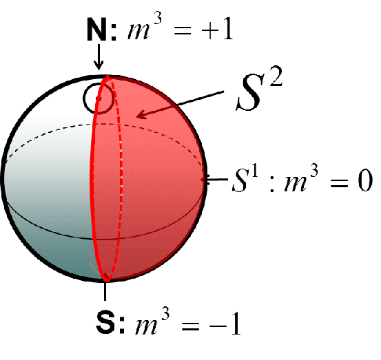
The configuration $\omega_{L}$ ($\omega_{L}^{*}$) goes to $n=(1,0)$ (${\bf m}=(0,0,1)$) denoted by $\odot$ at $x_{1}\to-\infty$ and to $n=(0,1)$ (${\bf m}=(0,0,-1)$) denoted by $\otimes$ at $x_{1}\to+\infty$. The configuration $\omega_{R}$ ($\omega_{R}^{*}$) goes to $n=(0,1)$ (${\bf m}=(0,0,-1)$) at $x_{1}\to-\infty$ and to $\omega=(1,0)$ (${\bf m}=(0,0,+1)$) at $x_{1}\to+\infty$. The configurations $\omega_{L}$ ($\omega_{L}^{*}$) and $\omega_{R}$ ($\omega_{R}^{*}$) can be regarded as a domain wall and anti-domain wall, respectively. A domain wall at each constant $x_{2}$ slice corresponds to a path connecting the north pole ${\bf m}=(0,0,+1)$ and the south pole ${\bf m}=(0,0,-1)$ in the target space, as illustrated in Fig. 2(a). A $U(1)$ modulus is localized on these domain walls characterizing which point on the equator in the target space a domain wall passes through [56]. This $U(1)$ modulus is twisted along the domain wall to satisfy the boundary condition at $x_{2}=0$ and $x_{2}=1$. When one changes a constant $x_{2}$ slice from $x_{2}=0$ to $x_{2}=1$, a path in the target space changes with sweeping a half of the sphere as the target space, as shown in Fig.2(b) and (c). Therefore, these configurations give maps from the space ${\mathbb{R}}\times S^{1}$ to a half of the target space.

BPS configurations $\omega_{L}$ and $\omega_{R}$ carry a half of the unit instanton charge, $Q=1/2$, while anti-BPS configurations $\omega_{L}^{*}$ and $\omega_{R}^{*}$ carry $Q=-1/2$. This fact also can be understood by noting that the $U(1)$ modulus is twisted half along the domain wall [57, 60].

Fractionalized instantons can exist in the ${\mathbb{C}}P^{N-1}$ model too. The configuration (18) of the ${\mathbb{C}}P^{1}$ model can be generalized into the $N$-vector $\omega$ for the ${\mathbb{C}}P^{N-1}$ model with the ${\mathbb{Z}}_{N}$ twisted boundary condition in Eq. (13) as

$\displaystyle\omega_{L}=\left(0,\cdots,0,1,\lambda e^{i\theta}e^{+2\pi z/N},0,\cdot\cdot\cdot\right)^{T}\,,\quad\omega_{R}=\left(0,\cdots,0,1,\lambda e^{i\theta}e^{-2\pi z/N},0,\cdot\cdot\cdot,0\right)^{T}\,.\quad$

(19)

A neutral bion configuration is a composite of a fractionalized instanton and fractionalized anti-intanton with the total instanton charge canceled out. Let us discuss the ${\mathbb{C}}P^{1}$ model first. From the solutions in Eq. (18) and their complex conjugates, it is reasonable to consider the following ansatz for the ${\mathbb{C}}P^{1}$ model satisfying a ${\mathbb{Z}}_{2}$ twisted boundary condition (13) as

$$\omega=\left(1+\lambda_{2}e^{i\theta_{2}}e^{\pi(z+\bar{z})},\,\,\lambda_{1}e^{i\theta_{1}}e^{\pi z}\right)^{T}\,,$$

(20)

constructed from fractionalized instantons $\omega_{L}$ and $\omega_{R}^{*}$ in Eq. (18). As we mentioned, the ansatz $\omega=e^{-\pi z/2}\left(1+\lambda_{2}e^{i\theta_{2}}e^{\pi(z+\bar{z})},\,\,\lambda_{1}e^{i\theta_{1}}e^{\pi z}\right)^{T}$ also gives the same ${\bf P}(x)$, thus these are equivalent. $\lambda_{1}\geq 0$, $\lambda_{2}\geq 0$, $0\leq\theta_{1},\theta_{2}<2\pi$ are all real parameters characterizing the configuration associated with this ansatz, as $\lambda_{1}^{2}/\lambda_{2}$ and $\lambda_{2}$ govern a relative separation and a center location between the instanton constituents respectively. We have no parameter characterizing the size of fractionalized instantons in the present ansatz. For $\lambda_{1}^{2}\gg\lambda_{2}$, this configuration is composed of two components, a BPS fractionalized instanton ($S=1/2$, $Q=1/2$) and a BPS fractionalized anti-instanton ($S=1/2$, $Q=-1/2$), which are separately located as shown in Fig. 3. Fig. 4 shows the action and topological charge densities of this configuration.

The superposition ansatz such as ours has been studied long for Yang-Mills instantons and ${\mathbb{C}}P^{N-1}$ instantons on $S^{2}$ and ${\mathbb{R}}^{2}$ (See [58] for example). On the other hand, for these theories, a multiple-type ansatz has been also investigated [59], in relation to the study on “zindons”. However, due to the fixed twisted boundary condition, it is not straightforward to construct an ansatz for the present case, with keeping, non-triviality of configurations, finite energy and the boundary conditions. The twisted boundary condition strongly restricts patterns of ansatz. This is why we begin with the simple ansatz (20).

It is notable that the action density and topological charge density are independent of $\theta_{1}$. The operators $\bf{P}$, $\partial_{z}{\bf P}$, $\partial_{\bar{z}}{\bf P}$, $\partial_{z}{\bf P}\partial_{\bar{z}}{\bf P}$ and $\partial_{\bar{z}}{\bf P}\partial_{z}{\bf P}$ have the following form as

$$\left(\begin{array}[]{cc}a&b\,e^{-i\theta_{1}}\\ c\,e^{+i\theta_{1}}&d\end{array}\right)\,,$$

(21)

where $a,b,c$ and $d$ are some functions of $z$ and $\bar{z}$ including $\lambda_{1},\lambda_{2}$ and $\theta_{2}$ as parameters. Then, it is obvious that both $s(x_{1})\sim{\rm Tr}[\partial_{z}{\bf P}\partial_{\bar{z}}{\bf P}]$ and $q(x_{1})={\rm Tr}[{\bf P}(\partial_{\bar{z}}{\bf P}\partial_{z}{\bf P}-\partial_{z}{\bf P}\partial_{\bar{z}}{\bf P})]$ have no $\theta_{1}$ dependence. It means that $\theta_{1}$ corresponds to a bosonic zero mode, which does not cost the configuration energy. On the other hand, the configuration depends on $\theta_{2}$. For now we assume $\theta_{2}=0$, and will consider $\theta_{2}\not=0$ cases later.

The total action and the net topological charge in the large-separation limit are given by

$$S=1,\,\,\,\,Q=0\,,$$

(22)

respectively. We note that the topological charge is zero for any values of separation, and this configuration corresponds to a topologically trivial vacuum.

Generalization of this configuration into the ${\mathbb{C}}P^{N-1}$ model is straightforward as

$$\omega=\left(0,\cdot\cdot\cdot,0,1+\lambda_{2}e^{i\theta_{2}}e^{2\pi(z+\bar{z})/N},\,\,\lambda_{1}e^{i\theta_{1}}e^{2\pi z/N},0,\cdot\cdot\cdot,0\right)^{T}\,.$$

(23)

The corresponding configuration again has no $\theta_{1}$ dependence. For $\lambda_{1}^{2}\gg\lambda_{2}$, this configuration corresponds to a $1/N$ instanton ($S=1/N$, $Q=1/N$) and a $1/N$ anti-instanton ($S=1/N$, $Q=-1/N$) at large separations. The total action and the net topological charge in this large-separation limit are given by

$$S=2/N,\,\,\,\,Q=0\,,$$

(24)

respectively.

As $x_{1}$ varies from $-\infty$ to $\infty$, the normalized complex vector $n(x_{1})$ takes the following three different values, which we denote as $n_{1},n_{2},n_{3}$,

$$n_{1}=(1,0,\cdot\cdot\cdot,0)^{T}\,\,\,\to\,\,\,n_{2}=(0,1,\cdot\cdot\cdot,0)^{T}\,\,\,\to\,\,\,n_{3}=(1,0,\cdot\cdot\cdot,0)^{T}\,,$$

(25)

for $\lambda_{1}^{2}>\lambda_{2}$. The above three domains are divided by two critical points corresponding to the locations of the two kinks. As shown in [9], the two affine co-roots $\alpha_{i}$ and $\alpha_{j}$, which correspond to the two kinks (fractionalized instantons) in Fig. 4 are given by

	$\displaystyle\alpha_{i}$	$\displaystyle=n_{2}-n_{1}\,,$		(26)
	$\displaystyle\alpha_{j}$	$\displaystyle=-(n_{3}-n_{2})\,,$		(27)

which satisfies

$$n(x_{1}=\infty)=n(x_{1}=-\infty)+\alpha_{i}-\alpha_{j}\,.$$

(28)

In the present case, $\alpha_{i}$ and $\alpha_{j}$ are identical, which we define as $\alpha_{i}=\alpha_{j}\equiv\alpha$. It is given by

$$\alpha\,=\,(0,1,\cdot\cdot\cdot,0)^{T}\,-\,(1,0,\cdot\cdot\cdot,0)^{T}\,=\,(-1,1,\cdot\cdot\cdot,0)^{T}\,.$$

(29)

We note that $\alpha_{i}\cdot\alpha_{j}=\alpha\cdot\alpha>0$ for this case.

The explicit form of the action density $s(x_{1})$ for general $N$ is given by

	$\displaystyle s(x_{1})=$	$\displaystyle{4\pi^{2}\over{N^{2}\left(1+(\lambda_{1}^{2}+2\lambda_{2}\cos\theta_{2})e^{4\pi x_{1}/N}+\lambda_{2}^{2}e^{8\pi x_{1}/N}\right)^{4}}}\,\times$
		$\displaystyle\Big[2(\lambda_{1}^{2}e^{4\pi x_{1}/N}-\lambda_{1}^{2}\lambda_{2}^{2}e^{12\pi x_{1}/N})^{2}$
		$\displaystyle+(\lambda_{1}e^{2\pi x_{1}/N}+2\lambda_{1}\lambda_{2}e^{i\theta_{2}}e^{6\pi x_{1}/N}+\lambda_{1}\lambda_{2}e^{i\theta_{2}}(\lambda_{1}^{2}+\lambda_{2}e^{i\theta_{2}})e^{10\pi x_{1}/N})\times$
		$\displaystyle\,\,\,\,\,\,\,(\lambda_{1}e^{2\pi x_{1}/N}+2\lambda_{1}\lambda_{2}e^{-i\theta_{2}}e^{6\pi x_{1}/N}+\lambda_{1}\lambda_{2}e^{-i\theta_{2}}(\lambda_{1}^{2}+\lambda_{2}e^{-i\theta_{2}})e^{10\pi x_{1}/N})$
		$\displaystyle+(\lambda_{1}(\lambda_{1}^{2}+\lambda_{2}e^{i\theta_{2}})e^{6\pi x_{1}/N}+2\lambda_{1}\lambda_{2}^{2}e^{10\pi x_{1}/N}+\lambda_{1}\lambda_{2}^{3}e^{-i\theta_{2}}e^{14\pi x_{1}/N})\times$
		$\displaystyle\,\,\,\,\,\,\,(\lambda_{1}(\lambda_{1}^{2}+\lambda_{2}e^{-i\theta_{2}})e^{6\pi x_{1}/N}+2\lambda_{1}\lambda_{2}^{2}e^{10\pi x_{1}/N}+\lambda_{1}\lambda_{2}^{3}e^{i\theta_{2}}e^{14\pi x_{1}/N})\Big]\,.$		(30)

Fig. 5 depicts the $\sqrt{\lambda_{1}^{2}/\lambda_{2}}$ dependence of the total action $S$ with $\theta_{2}=0$ for $N=2$.

We will from now look into the attractive interaction between the two fractionalized instantons. In order to understand precise separation dependence of action and interaction force, we need to know the exact separation between the two components of fractionalized instantons in our configuration. The positions $\tau_{1}$ and $\tau_{2}$ of fractionalized instantons and fractionalized anti-instantons in the $x_{1}$-coordinate are given by the balance conditions [44, 61, 45, 62],

		$\displaystyle 1=\lambda_{1}e^{2\pi\tau_{1}/N}\,\,\,\,\,\,\,\,\,\to\,\,\,\,\,\,\,\,\,\tau_{1}={N\over{2\pi}}\log\left({1\over{\lambda_{1}}}\right)\,,$		(31)
		$\displaystyle\lambda_{2}e^{4\pi\tau_{2}/N}=\lambda_{1}e^{2\pi\tau_{2}/N}\,\,\,\,\,\,\,\,\,\to\,\,\,\,\,\,\,\,\,\tau_{2}={N\over{2\pi}}\log\left({\lambda_{1}\over{\lambda_{2}}}\right)\,,$		(32)

respectively. Then, the separation $\tau$ between them is given by

$$\tau=\tau_{2}-\tau_{1}={N\over{2\pi}}\log\left({\lambda_{1}^{2}\over{\lambda_{2}}}\right)\,.$$

(33)

For $\tau\geq 0$, $\tau$ can be interpreted as separation between the fractionalized-instanton components. The definition of separation depends on $N$ for this configuration. As noted in the caption in Fig. 4, this definition of separation precisely describes the distance between the locations of two fractionalized instantons.

Fig. 6 depicts the separation $\tau$ dependence of the total action $S$ and the static force $F=-{dS\over{d\tau}}$ with $\lambda_{2}=1$ fixed for $N=2$. It indicates that the total action monotonically decreases as $\tau$ gets smaller, and the interaction force is negative for wide $\tau$ range. It clearly shows that the fractionalized-instanton constituents exert an attractive force. To be precise, as will be shown later, the interaction force is exponentially suppressed for large separation $\tau\gg 1$ or the merged limit $\tau\ll 0$ ($\lambda_{1}^{2}/\lambda_{2}\ll 1$). It indicates that our ansatz yields intermediate configurations between two (approximate) solutions, a two-separated fractionalized-instanton solution ($S=1$, $Q=0$) and a trivial perturbative vacuum ($S=0$, $Q=0$). Our analysis is easily generalized to $\lambda_{2}\not=1$, where we find that the total action is independent of $\lambda_{2}$ if $\lambda_{1}^{2}/\lambda_{2}$ or $\tau$ are fixed. From this analysis, we see that the location of the center of mass $\lambda_{2}$ corresponds to a bosonic zero mode while $\lambda_{1}^{2}/\lambda_{2}$ to a negative mode.

The two constituents are getting closer and finally are merged by the attractive force, as shown in Fig. 7. The resultant configuration at $\tau=-\infty$ ($\lambda_{1}^{2}/\lambda_{2}=0$) is given by

$$\omega(\tau=-\infty)\,\to\,\left(1+\lambda_{2}e^{\pi(z+\bar{z})},\,\,0\right)^{T}\,,$$

(34)

for $N=2$, and

$$\omega(\tau=-\infty)\,\to\,\left(0,\cdot\cdot\cdot,0,1+\lambda_{2}e^{i\theta_{2}}e^{2\pi(z+\bar{z})/N},\,\,0,0,\cdot\cdot\cdot,0\right)^{T}\,.$$

(35)

for general $N$, with the quantum number

$$S=0,\,\,\,\,Q=0\,,$$

(36)

which is identical to a trivial vacuum.

Here we discuss the characteristic size of neutral bions. As shown in [9], the size of “charged” bions $N_{f}>0$ is clearly determined since the instanton constituents are bound due to the balance of bosonic repulsive and fermionic attractive forces. This calculation can be extended to the case of $N_{f}=0$, and it gives the length scale of charged bions as $\tau^{\ast}={N\over{2\pi}}\log{8\pi\over{g^{2}N}}$, which reads $\tau^{\ast}=0.5\sim 1.5$ for $N=O(1)$ with $g^{2}=1$. On the other hand, the calculation of the neutral bion size is not straightforward since its bosonic interaction is attractive and it requires analytic continuation of $g^{2}$ to negative values and its returning back to positive values. However, taking into account the fact that the actions of neutral and charged bions in the amplitudes are common except for the imaginary part, we speculate that neutral bions have a similar size or length scale to that of the charged bions $\tau^{\ast}\sim 1$. In the rest of the paper, we assume that the neutral bions arise from the separation scale $\tau\gtrsim 1$. We thus regard our ansatz as the neutral bions only for the separation $\tau>1$. We will discuss whether this assumption is appropriate or not in terms of BZJ-prescription in Sec. V.

We now investigate interaction part of the action for this configuration, to compare our concrete ansatz to the far-separated instanton argument (1) in Ref. [9]. The interaction part of the action density is written as the action density $s(x_{1})$ minus the one fractionalized-instanton density and one fractionalized-anti-instanton density $s_{\nu=1/N}(x_{1})+s_{\nu=-1/N}(x_{1})$,

$$s_{\rm int}(x_{1})=s(x_{1})-(s_{\nu=1/N}(x_{1})+s_{\nu=-1/N}(x_{1}))\,.$$

(37)

The integrated interaction action is then given by

$$S_{\rm int}(N,\tau)\,=\,{1\over{\pi}}\int dx\,s_{\rm int}(x_{1})\,.$$

(38)

In Fig. 8, we plot the logarithm of the total interaction action $S_{\rm int}(N,\tau)$ as a function of $\tau$ for $N=2,3,4$. For $\tau\gtrsim 1$ region, $\log(-S_{\rm int}(N,\tau))$ can be well approximated by analytic lines,

$$\log\left[-S_{\rm int}(N,\tau)\right]\,\,\sim\,\,-\xi(N)\,\tau\,\,+\,\,C(N)\,,\,\,\,\,\,\,\,\,\,\,\,\,\,\,\,\,\,(\tau\gtrsim 1)\,,$$

(39)

where $\xi(N)$ is a slope and $C(N)$ is a $y$-intercept. In Fig. 8 we simultaneously depict these analytic lines for the three cases. The slopes $\xi$ of the approximate lines read $\xi\sim\pi$ for $N=2$, $\xi\sim 2\pi/3$ for $N=3$ and $\xi\sim\pi/2$ for $N=4$, which indicates that the slope $\xi$ can be generally expressed as

$$\xi(N)\,\sim\,{2\pi\over{N}}\,.$$

(40)

Therefore we observe that the interaction action can be written as the following form for $\tau\gtrsim 1$ region,

$$S_{\rm int}(N,\tau)\,\,\sim\,\,-\,e^{C}\,e^{-\xi\tau}\,,\,\,\,\,\,\,\,\,\,\,\,\xi={2\pi\over{N}}\,,\,\,\,\,\,\,\,\,\,\,\,\,\,\,\,\,\,(\tau\gtrsim 1)\,.$$

(41)

This $\xi$ is equivalent to the (dimensionless) lowest Kaluza-Klein spectrum $Lm_{LKK}$, which is given as $Lm_{LKK}=|q_{i}-q_{j}|=2\pi/N$, where $q_{i}$ and $q_{j}$ are two nonzero components of Wilson-loop holonomy in (14)(15).

We next determine the $N$ dependence of the $y$-intercept $C(N)$. In Fig. 9 we plot exponential of the intercept $\exp[{C(N)}]$ as a function of $N$ for $N=2,3,4,5,6,7$. We find out that this dependence is well approximated by $\exp[C(N)]\sim 4/N$, and depict it simultaneously in the figure. This result shows that the interaction action for $\tau\gtrsim 1$ can be written as

$$S_{\rm int}(N,\tau)\,\,\sim\,\,-{4\over{N}}\,e^{-\xi\tau}\,,\,\,\,\,\,\,\,\,\,\,\,\xi={2\pi\over{N}}\,,\,\,\,\,\,\,\,\,\,\,\,\,\,\,\,\,\,(\tau\gtrsim 1)\,.$$

(42)

It means, for a wide range of separations $\tau\gtrsim 1$, the interaction part of the action for our configuration is consistent with the neutral bion action (1) obtained from the far-separated instanton calculation up to $2\pi$ factor, which we introduced for convenience, as

$$S_{\rm int}(N,\tau)=-4\xi\,(\alpha_{i}\cdot\alpha_{j})\,e^{-\xi\tau}=-{8\pi\over{N}}e^{-\xi\tau}\,,\,\,\,\,\,\,\,\,\,\,\,\xi={2\pi\over{N}}\,,$$

(43)

with $\alpha_{i}\cdot\alpha_{j}=\alpha\cdot\alpha=1$ for our ansatz following the Lie algebra notation in [9].

We have shown that our ansatz (20) gives a configuration consistent to (1) except in the merged region $\tau<1$. It means that (20) is a good ansatz describing the neutral bion, and can be identified as an infrared renormalon since the imaginary part of its amplitude obtained through the BZJ-prescription ($g^{2}\to-g^{2}$) and analytic continuation cancels the notorious ambiguity arising in the Borel re-summation of the perturbative series. By use of the present ansatz, we can study properties of bions and the related physics, not only at large separation $\tau\gg 1$, but also at short separation $\tau\gtrsim 1$.

We here discuss a physical meaning of our ansatz for the merged region $\tau<1$. The coincidence of the interactive actions for $\tau\gtrsim 1$ (Fig. 8) implies that the neutral bion scale can be determined by such a coincidence point, or $\tau\sim 1$ for this case, which is consistent with the charged bion scale. On the other hand, for the region $\tau<1$, the configurations (see the right two columns in Fig. 7) are regarded as those around the perturbative vacuum rather than the bion saddle. It means that, in the semi-classical calculation, these configurations correspond to fluctuations around the perturbative saddle, but not around the bion saddle point. It is also notable that our ansatz connects these two different saddle points continuously by a single parameter. We will briefly discuss how to classify the parameter regions into the two sectors in Sec. V.

We here make a comment on cases for $\theta_{2}\not=0$. For $0<\theta_{2}<\pi/2$, the interaction force is qualitatively the same as the case for $\theta_{2}=0$, or attractive. For $\pi/2\leq\theta_{2}\leq\pi$, things change: The potential barrier emerges around $\sqrt{\lambda_{1}^{2}/\lambda_{2}}=1$ ($\tau=0$), and the height becomes infinite for $\theta_{2}=\pi$ as shown in Fig. 10. Of course, this does not mean that the interaction is repulsive since $\theta_{2}$ is also a dynamical field variable and should relax eventually to $\theta_{2}=0$ in order to minimize the total action. The result indicates that $\theta_{2}$ corresponds to a positive mode.

We first consider a configuration in ${\mathbb{C}}P^{2}$ satisfying the split twisted boundary condition (44),

$$\omega=\left(1,\,\,\lambda_{2}e^{i\theta_{2}}e^{\pi(z+\bar{z})},\,\,\lambda_{1}e^{i\theta_{1}}e^{\pi z}\right)^{T}\,,$$

(46)

This is an ansatz beyond the simple superposition ansatz. For $\lambda_{1}^{2}\gg\lambda_{2}$, this configuration is composed of a BPS fractionalized instanton ($S=1/2$, $Q=1/2$) and a BPS fractionalized anti-instanton ($S=1/2$, $Q=-1/2$) in Fig. 11. The total action and the net topological charge in a far-separated limit are given by

$$S=1,\,\,\,\,Q=0\,.$$

(47)

We note the action density and topological charge density are independent of the parameters $\theta_{1}$ and $\theta_{2}$. Fig. 12 depicts $\sqrt{\lambda_{1}^{2}/\lambda_{2}}$ dependence of the total action $S$ for (46). The total action is independent of $\lambda_{2}$ with $\lambda_{1}^{2}/\lambda_{2}$ fixed.

For this ansatz, the normalized complex vector $n(x_{1})$ takes the following three different values as $x_{1}$ varies from $-\infty$ to $\infty$,

$$n_{1}=(1,0,0)^{T}\,\,\,\to\,\,\,n_{2}=(0,0,1)^{T}\,\,\,\to\,\,\,n_{3}=(0,1,0)^{T}\,,$$

(48)

for $\lambda_{1}^{2}>\lambda_{2}$. For this case, the entry of extended Cartan matrix is again positive $\alpha_{i}\cdot\alpha_{j}>0$

The separation $\tau$ is given by

$$\tau={1\over{\pi}}\log\left({\lambda_{1}^{2}\over{\lambda_{2}}}\right)\,,$$

(49)

which is obtained from the balance conditions [44, 61, 45, 62],

		$\displaystyle 1=\lambda_{1}e^{\pi\tau_{1}}\,\,\,\,\,\,\,\,\,\to\,\,\,\,\,\,\,\,\,\tau_{1}={1\over{\pi}}\log\left({1\over{\lambda_{1}}}\right)\,,$		(50)
		$\displaystyle\lambda_{2}e^{2\pi\tau_{2}}=\lambda_{1}e^{\pi\tau_{2}}\,\,\,\,\,\,\,\,\,\to\,\,\,\,\,\,\,\,\,\tau_{2}={1\over{\pi}}\log\left({\lambda_{1}\over{\lambda_{2}}}\right)\,,$		(51)

with $\tau=\tau_{2}-\tau_{1}$. For $\tau\geq 0$, $\tau$ stands for a separation between the fractionalized-instanton constituents. In Fig. 13 we depicts $\tau$ dependence of the total action $S$ and the static force $F=-{dS\over{d\tau}}$ for (46). The result indicates that the force is negative for $-\infty<\tau<\infty$, and the fractionalized instanton constituents have an attractive force. As with the configuration in the previous section, the two fractionalized instantons are merged by the attractive force, and finally resulting in the configuration,

$$\omega(\tau=-\infty)\,\,\to\,\,\left(1,\,\,\lambda_{2}e^{i\theta_{2}}e^{\pi(z+\bar{z})},\,\,0\right)^{T}\,,$$

(52)

at $\tau=-\infty$ ($\lambda_{1}^{2}/\lambda_{2}=0$) with

$$S=1/2,\,\,\,\,Q=0\,.$$

(53)

From this analysis, we see that $\lambda_{2}$, $\theta_{1}$ and $\theta_{2}$ correspond to bosonic zero modes while $\lambda_{1}^{2}/\lambda_{2}$ to a negative mode.