跳到论文正文
W Papers独立论文阅读器 arXiv:1404.7209 论文正文 计算阅读时间 · 0%
引用这篇论文根据当前论文元数据生成,正式投稿前建议核对。


License: arXiv.org perpetual non-exclusive license
arXiv:1404.7209v2 [math.OC] 25 May 2015

A max-plus dual space fundamental solution for a class of operator differential Riccati equationsThanks:  This research is supported by grants from the Australian Research Council, AFOSR, and NSF. Preliminary results contributing to this paper appear in [9, 10, 11].

Peter M. Dower ††thanks: Department of Electrical & Electronic Engineering, University of Melbourne, Victoria 3010, Australia. pdower@unimelb.edu.au, +61-3-8344-6711.    William M. McEneaney ††thanks: Department of Mechanical & Aerospace Engineering, University of California at San Diego, 9500 Gilman Dr., La Jolla, CA 92093-0411, USA. wmceneaney@eng.ucsd.edu, +1-858-822-5835.
Abstract

A new fundamental solution semigroup for operator differential Riccati equations is developed. This fundamental solution semigroup is constructed via an auxiliary finite horizon optimal control problem whose value functional growth with respect to time horizon is determined by a particular solution of the operator differential Riccati equation of interest. By exploiting semiconvexity of this value functional, and the attendant max-plus linearity and semigroup properties of the associated dynamic programming evolution operator, a semigroup of max-plus integral operators is constructed in a dual space defined via the Legendre-Fenchel transform. It is demonstrated that this semigroup of max-plus integral operators can be used to propagate all solutions of the operator differential Riccati equation that are initialized from a specified class of initial conditions. As this semigroup of max-plus integral operators can be identified with a semigroup of quadratic kernels, an explicit recipe for the aforementioned solution propagation is also rendered possible.

keywords
Infinite dimensional systems, operator differential Riccati equations, fundamental solution, semigroups, max-plus methods, Lengendre-Fenchel transform, optimal control.
AMS
49L20, 49M29, 15A80, 93C20, 47F05, 47D06.

1 Introduction

The objective of this paper is to develop a new fundamental solution semigroup for operator differential Riccati equations of the form

𝒫˙​(t)\displaystyle\dot{{\mathcal{P}}}(t) =𝒫⁡(t)​𝒜+𝒜′​𝒫​(t)+𝒫⁡(t)​σ​σ′​𝒫​(t)+𝒞,\displaystyle={\mathcal{P}}(t)\,{\mathcal{A}}+{\mathcal{A}}^{\prime}\,{\mathcal{P}}(t)+{\mathcal{P}}(t)\,\sigma\,\sigma^{\prime}\,{\mathcal{P}}(t)+{\mathcal{C}}\,, (1)

where 𝒫⁡(t){\mathcal{P}}(t) is a self-adjoint bounded linear operator evolved to time tt from some initialization 𝒫⁡(0){\mathcal{P}}(0), 𝒜{\mathcal{A}} is an unbounded, densely defined and boundedly invertible linear operator that generates a C0C_{0}-semigroup of bounded linear operators, and σ\sigma and 𝒞{\mathcal{C}} are bounded linear operators, all defined with respect to a pair of underlying Hilbert spaces 𝒳{\mathscr{X}} and 𝒲{\mathscr{W}}. Operator differential Riccati equations of this form arise naturally in the formulation and solution of optimal control problems for linear infinite dimensional systems [7, 8]. Their solution is of particular interest where a state feedback characterization for an optimal control is sought. The fundamental solution semigroup obtained generalizes the finite dimensional case presented in [17], and the specific infinite dimensional cases documented in [9, 10] for mild solutions. It describes all solutions of (1) corresponding to a class of quadratic terminal payoffs. Preliminary results in this direction also appear in [11].

Development of the new fundamental solution semigroup for (1) proceeds by considering an infinite dimensional optimal control problem on a finite time horizon tt. This control problem is constructed such that the value functional obtained exhibits quadratic growth with respect to the state variable, where the growth is determined by the solution 𝒫⁡(t){\mathcal{P}}(t) of the operator differential Riccati equation (1) at time tt. Consequently, evolution of the solution 𝒫⁡(t){\mathcal{P}}(t) of (1) with time tt can be identified with evolution of the value functional with respect to time horizon tt, with dynamic programming [4, 5] providing a mechanism for the latter. As the value functional obtained is demonstrably semiconvex, its evolution via dynamic programming can be identified with a corresponding evolution in a dual space defined via the Legendre-Fenchel transform [20]. Critically, by exploiting max-plus linearity of the dynamic programming evolution operator, this dual space evolution can be decoupled from the terminal payoff employed in the optimal control problem, and hence from the initial data that defines any specific solution 𝒫{\mathcal{P}} of (1). Indeed, the set of time horizon indexed dual space evolution operators defined via this decoupling describes a fundamental solution to (1), as its elements can be used to propagate any initial data 𝒫⁡(0){\mathcal{P}}(0) within a specific class of operators to yield the corresponding solution 𝒫⁡(t){\mathcal{P}}(t) of (1) at time t∈ℝ≥0t\in{\mathbb{R}}_{\geq 0}. As dynamic programming naturally endows the value functional with a semigroup property, this set of time horizon indexed dual space evolution operators also defines a semigroup that can be regarded as the max-plus dual space fundamental solution semigroup for (1).

In terms of organization, the operator differential Riccati equation of interest is posed in Section 2, along with results concerning existence and uniqueness of its solution on a finite time horizon. Construction of the max-plus fundamental solution semigroup is presented in detail in Section 3, with the steps involved in applying this fundamental solution semigroup to evaluate solutions of (1) enumerated in Section 4. This is followed by some brief conclusions in Section 5, and appendices that include (for completeness) pertinent well-known details concerning continuity of operator-valued functions, the Yosida approximation, and so on.

2 Operator differential Riccati equation

Attention is initially restricted to the operator differential Riccati equation (1) of interest, with sufficient conditions for existence and uniqueness of solutions on a finite horizon established following the approach of [7]. Two auxiliary operator differential equations of subsequent utility are similarly considered. In generalizing the finite dimensional Riccati equations considered in [17], the main technical challenges in the infinite dimensional setting considered here concern the notion of solution for operator differential equations, the consequences of an unbounded 𝒜{\mathcal{A}} in analyzing those equations and solutions, and an appropriate notion of semiconvexity for functionals on infinite dimensional spaces. Tools for dealing with these challenges are well-understood, and are cited directly from [7, 8, 18] and [2, 14, 20] as required. Otherwise, the development largely follows that of the finite dimensional case [17].

2.1 Riccati equation

Consider the operator differential Riccati equation posed with respect to Hilbert spaces 𝒳{\mathscr{X}} and 𝒲{\mathscr{W}} by

𝒫˙​(t)\displaystyle{\dot{{\mathcal{P}}}}(t) =𝒜′​𝒫​(t)+𝒫⁡(t)​𝒜+𝒫⁡(t)​σ​σ′​𝒫​(t)+𝒞,\displaystyle={\mathcal{A}}^{\prime}\,{\mathcal{P}}(t)+{\mathcal{P}}(t)\,{\mathcal{A}}+{\mathcal{P}}(t)\,\sigma\,\sigma^{\prime}\,{\mathcal{P}}(t)+{\mathcal{C}}\,, (1)

in which 𝒜:dom​(𝒜)⊂𝒳→𝒳{\mathcal{A}}:{\textsf{dom}}({\mathcal{A}})\subset{\mathscr{X}}\rightarrow{\mathscr{X}} is unbounded and densely defined on 𝒳{\mathscr{X}}, σ∈ℒ⁡(𝒲,𝒳)\sigma\in{\mathcal{L}}({\mathscr{W}};{\mathscr{X}}), 𝒞∈ℒ⁡(𝒳){\mathcal{C}}\in{\mathcal{L}}({\mathscr{X}}) is self-adjoint and non-negative, 𝒜′{\mathcal{A}}^{\prime} and σ′\sigma^{\prime} denote the respective adjoints of 𝒜{\mathcal{A}} and σ\sigma, and t∈[0,τ∗]t\in[0,\tau^{*}] for some τ∗∈ℝ>0\tau^{*}\in{\mathbb{R}}_{>0}. (Throughout, ℒ⁡(𝒳,𝒴){\mathcal{L}}({\mathscr{X}};{\mathscr{Y}}) is used to denote the space of bounded linear operators mapping from Banach space 𝒳{\mathscr{X}} to Banach space 𝒴{\mathscr{Y}}. Where 𝒳=𝒴{\mathscr{X}}={\mathscr{Y}}, this notation is abbreviated to ℒ⁡(𝒳){\mathcal{L}}({\mathscr{X}}).)

Assumption 1.

𝒜{\mathcal{A}} is boundedly invertible and generates a C0C_{0}-semigroup of bounded linear operators.

In order to define solutions for the operator differential Riccati equation (1), it is convenient [7] to define two sets of self-adjoint bounded linear operators by

Σ⁡(𝒳)\displaystyle\Sigma({\mathscr{X}}) ≐{𝒫∈ℒ⁡(𝒳)|𝒫​ is self-adjoint},\displaystyle\doteq\left\{{\mathcal{P}}\in{\mathcal{L}}({\mathscr{X}})\,\biggl|\,{\mathcal{P}}\text{ is self-adjoint}\right\}, (2)
Σℳ​(𝒳)\displaystyle\Sigma_{{\mathcal{M}}}({\mathscr{X}}) ≐{𝒫∈Σ(𝒳)|𝒫−ℳ​ is coerciveon dom​(𝒜)},ℳ∈Σ(𝒳).\displaystyle\doteq\left\{{\mathcal{P}}\in\Sigma({\mathscr{X}})\,\left|\begin{array}[]{c}{\mathcal{P}}-{\mathcal{M}}\text{ is coercive}\\ \text{on }{\textsf{dom}}({\mathcal{A}})\end{array}\right.\right\},\quad{\mathcal{M}}\in\Sigma({\mathscr{X}})\,.

An operator 𝒫:dom​(𝒫)⊂𝒳→𝒳{\mathcal{P}}:{\textsf{dom}}({\mathcal{P}})\subset{\mathscr{X}}\rightarrow{\mathscr{X}} is coercive if there exists an ϵ∈ℝ>0{\epsilon}\in{\mathbb{R}}_{>0} such that ⟨x,𝒫​x⟩≥ϵ​‖x‖2\langle x,\,{\mathcal{P}}\,x\rangle\geq{\epsilon}\,\|x\|^{2} for all x∈dom​(𝒫)x\in{\textsf{dom}}({\mathcal{P}}). If 𝒫{\mathcal{P}} is both coercive and self-adjoint, then it has a bounded inverse, see [8, Example A.4.2, p.609] and [15, Problem 10, p.535].

Relevant spaces of (uniformly) continuous and strongly continuous operator-valued functions defined on an interval I≐[0,T]⊂ℝ≥0I\doteq[0,T]\subset{\mathbb{R}}_{\geq 0}, T∈ℝ>0T\in{\mathbb{R}}_{>0}, and taking values in Σ∈{ℒ⁡(𝒳),Σ⁡(𝒳),Σℳ​(𝒳)}\Sigma\in\{{\mathcal{L}}({\mathscr{X}}),\,\Sigma({\mathscr{X}}),\,\Sigma_{{\mathcal{M}}}({\mathscr{X}})\}, are

C⁡(I,Σ)\displaystyle C(I;\Sigma) ≐{ℱ:I→Σ|ℱ​ iscontinuous},\displaystyle\doteq\left\{{\mathcal{F}}:I\rightarrow\Sigma\,\left|\begin{array}[]{c}{\mathcal{F}}\text{ is}\\ \text{continuous}\end{array}\right.\right\},
C0​(I,Σ)\displaystyle C_{0}(I;\Sigma) ≐{ℱ:I→Σ|ℱ​ is stronglycontinuous}.\displaystyle\doteq\left\{{\mathcal{F}}:I\rightarrow\Sigma\,\left|\begin{array}[]{c}{\mathcal{F}}\text{ is strongly}\\ \text{continuous}\end{array}\right.\right\}\,.
Remark 2.2.

Any bounded linear operator is the generator of a uniformly continuous semigroup of bounded linear operators (see [18, Theorem 1.2, p.2]). In constrast, the unbounded and densely defined operator 𝒜:dom​(𝒜)⊂𝒳→𝒳{\mathcal{A}}:{\textsf{dom}}({\mathcal{A}})\subset{\mathscr{X}}\rightarrow{\mathscr{X}} of (1) is the generator of a strongly (C0C_{0}-) semigroup of bounded linear operators by Assumption 1 (which also implies that 𝒜{\mathcal{A}} is closed, see also [18, Corollary 2.5, p.5]). These semigroups are subsets of C⁡(I,ℒ⁡(𝒳))C(I;{\mathcal{L}}({\mathscr{X}})) and C0​(I,ℒ​(𝒳))C_{0}(I;{\mathcal{L}}({\mathscr{X}})) respectively. Elements of such a semigroup, denoted by e𝒜​te^{{\mathcal{A}}\,t} for t∈ℝ≥0t\in{\mathbb{R}}_{\geq 0}, satisfy the usual semigroup properties, with e𝒜​ 0=ℐe^{{\mathcal{A}}\,0}={\mathcal{I}} (the identity operator), and e𝒜​t​e𝒜​s=e𝒜⁡(t+s)=e𝒜​s​e𝒜​te^{{\mathcal{A}}\,t}\,e^{{\mathcal{A}}\,s}=e^{{\mathcal{A}}\,(t+s)}=e^{{\mathcal{A}}\,s}\,e^{{\mathcal{A}}\,t} for all s,t∈ℝ≥0s,t\in{\mathbb{R}}_{\geq 0} such that s,t,s+t∈Is,t,s+t\in I. (See also Remark 3.16.) Note finally that C⁡(I,Σ)⊂C0​(I,Σ)C(I;\Sigma)\subset C_{0}(I;\Sigma) for Σ∈{ℒ⁡(𝒳),Σ⁡(𝒳),Σℳ​(𝒳)}\Sigma\in\{{\mathcal{L}}({\mathscr{X}}),\,\Sigma({\mathscr{X}}),\,\Sigma_{{\mathcal{M}}}({\mathscr{X}})\}, where C⁡(I,Σ⁡(𝒳))⊂C⁡(I,ℒ⁡(𝒳))C(I;\Sigma({\mathscr{X}}))\subset C(I;{\mathcal{L}}({\mathscr{X}})) and C0​(I,Σ⁡(𝒳))⊂C0​(I,ℒ⁡(𝒳))C_{0}(I;\Sigma({\mathscr{X}}))\subset C_{0}(I;{\mathcal{L}}({\mathscr{X}})) define vector spaces, while C​(I,Σℳ​(𝒳))C(I;\Sigma_{\mathcal{M}}({\mathscr{X}})) and C0​(I,Σℳ​(𝒳))C_{0}(I;\Sigma_{\mathcal{M}}({\mathscr{X}})) are merely subsets of those vector spaces. (See Appendix A.)

A mild solution of the operator differential Riccati equation (1) on a time interval [0,T][0,T], T∈ℝ>0T\in{\mathbb{R}}_{>0}, is any operator-valued function 𝒫∈C0​([0,T],Σ⁡(𝒳)){\mathcal{P}}\in C_{0}([0,T];\Sigma({\mathscr{X}})) that satisfies

𝒫⁡(t)​x\displaystyle{\mathcal{P}}(t)\,x =γ​(𝒫)​(t)​x,\displaystyle=\gamma({\mathcal{P}})(t)\,x\,, (9)

for all x∈𝒳x\in{\mathscr{X}}, t∈[0,T]t\in[0,T], with γ⁡(𝒪)\gamma({\mathcal{O}}) defined for every 𝒪∈C0​([0,T],Σ⁡(𝒳)){\mathcal{O}}\in C_{0}([0,T];\Sigma({\mathscr{X}})) by

[γ⁡(𝒪)​(t)]​x≐e𝒜′​t​𝒪​(0)​e𝒜​t​x+∫0te𝒜′​(t−s)​[𝒪⁡(s)​σ​σ′​𝒪​(s)+𝒞]​e𝒜⁡(t−s)​x​𝑑s\displaystyle\left[\gamma({\mathcal{O}})(t)\right]x\doteq e^{{\mathcal{A}}^{\prime}\,t}\,{\mathcal{O}}(0)\,e^{{\mathcal{A}}\,t}\,x+\int_{0}^{t}e^{{\mathcal{A}}^{\prime}\,(t-s)}\left[{\mathcal{O}}(s)\,\sigma\,\sigma^{\prime}\,{\mathcal{O}}(s)+{\mathcal{C}}\right]e^{{\mathcal{A}}\,(t-s)}\,x\,ds (10)

for all t∈[0,T]t\in[0,T], x∈𝒳x\in{\mathscr{X}}, where e𝒜′⋅e^{{\mathcal{A}}^{\prime}\,\cdot} denotes the C0C_{0}-semigroup generated by the operator adjoint 𝒜′{\mathcal{A}}^{\prime} (see, for example, [8, Theorem 2.2.6, p.37]). As per [7], it is convenient to introduce an analogous operator differential Riccati equation to (1), defined with respect to the Yosida approximations 𝒜n∈ℒ⁡(𝒳){\mathcal{A}}_{n}\in{\mathcal{L}}({\mathscr{X}}) of 𝒜{\mathcal{A}} defined for all n∈ℕn\in{\mathbb{N}}, see Appendix B. In particular,

𝒫˙n​(t)\displaystyle{\dot{{\mathcal{P}}}}_{n}(t) =𝒜n′​𝒫n​(t)+𝒫n​(t)​𝒜n+𝒫n​(t)​σ​σ′​𝒫n​(t)+𝒞.\displaystyle={\mathcal{A}}_{n}^{\prime}\,{\mathcal{P}}_{n}(t)+{\mathcal{P}}_{n}(t)\,{\mathcal{A}}_{n}+{\mathcal{P}}_{n}(t)\,\sigma\,\sigma^{\prime}\,{\mathcal{P}}_{n}(t)+{\mathcal{C}}\,. (11)

Similarly, a solution of (11) on a time interval [0,T][0,T], T∈ℝ>0T\in{\mathbb{R}}_{>0}, is any operator-valued function 𝒫n∈C⁡([0,T],Σ⁡(𝒳)){\mathcal{P}}_{n}\in C([0,T];\Sigma({\mathscr{X}})) that satisfies

𝒫n​(t)​x\displaystyle{\mathcal{P}}_{n}(t)\,x =γn​(𝒫n)​(t)​x,\displaystyle=\gamma_{n}({\mathcal{P}}_{n})(t)\,x\,, (12)

for all x∈𝒳x\in{\mathscr{X}}, t∈[0,T]t\in[0,T], with γn​(𝒪)\gamma_{n}({\mathcal{O}}) defined for every 𝒪∈C⁡([0,T],Σ⁡(𝒳)){\mathcal{O}}\in C([0,T];\Sigma({\mathscr{X}})) by

[γn​(𝒪)​(t)]​x≐e𝒜n′​t​𝒪​(0)​e𝒜n​t​x+∫0te𝒜n′​(t−s)​[𝒪⁡(s)​σ​σ′​𝒪​(s)+𝒞]​e𝒜n​(t−s)​x​𝑑s\displaystyle\left[\gamma_{n}({\mathcal{O}})(t)\right]x\doteq e^{{\mathcal{A}}_{n}^{\prime}\,t}\,{\mathcal{O}}(0)\,e^{{\mathcal{A}}_{n}\,t}\,x+\int_{0}^{t}e^{{\mathcal{A}}_{n}^{\prime}\,(t-s)}\left[{\mathcal{O}}(s)\,\sigma\,\sigma^{\prime}\,{\mathcal{O}}(s)+{\mathcal{C}}\right]e^{{\mathcal{A}}_{n}\,(t-s)}\,x\,ds (13)

for all t∈[0,T]t\in[0,T], x∈𝒳x\in{\mathscr{X}}, where e𝒜n′​t∈ℒ⁡(𝒳)e^{{\mathcal{A}}_{n}^{\prime}\,t}\in{\mathcal{L}}({\mathscr{X}}) denotes an element of the uniformly continuous semigroup generated by the Yosida approximation adjoint 𝒜n′∈ℒ⁡(𝒳){\mathcal{A}}_{n}^{\prime}\in{\mathcal{L}}({\mathscr{X}}).

Remark 2.3.

Equations (9) and (12) are integral equations that may be derived formally from their operator differential Riccati equation counterparts (1) and (11), respectively, see Appendix D.

Theorem 2.4.

Given any 𝒫0∈Σ⁡(𝒳){\mathcal{P}}_{0}\in\Sigma({\mathscr{X}}), there exists a τ∈ℝ>0\tau\in{\mathbb{R}}_{>0} such that the operator differential Riccati equations (1), (11) exhibit respective unique solutions 𝒫∈C0​([0,τ],Σ⁡(𝒳)){\mathcal{P}}\in C_{0}([0,\tau];\Sigma({\mathscr{X}})), 𝒫n∈C⁡([0,τ],Σ⁡(𝒳)){\mathcal{P}}_{n}\in C([0,\tau];\Sigma({\mathscr{X}})) satisfying 𝒫⁡(0)=𝒫0=𝒫n​(0){\mathcal{P}}(0)={\mathcal{P}}_{0}={\mathcal{P}}_{n}(0) for all n∈ℕn\in{\mathbb{N}}. Furthermore, for all x∈𝒳x\in{\mathscr{X}},

limn→∞𝒫n​(⋅)​x=𝒫⁡(⋅)​x,\displaystyle\lim_{n\rightarrow\infty}{\mathcal{P}}_{n}(\cdot)\,x={\mathcal{P}}(\cdot)\,x\,, (14)

where the limit is defined with respect to the Banach space (C([0,τ];𝒳),∥⋅∥C⁡([0,τ],𝒳))(C([0,\tau];{\mathscr{X}}),\,\|\cdot\|_{C([0,\tau];{\mathscr{X}})}), in which ‖x‖C⁡([0,τ],𝒳)≐supt∈[0,τ]‖x⁡(t)‖\|x\|_{C([0,\tau];{\mathscr{X}})}\doteq\sup_{t\in[0,\tau]}\|x(t)\| for all x∈C⁡([0,τ],𝒳)x\in C([0,\tau];{\mathscr{X}}).

Remark 2.5.

The limit (14) is a statement of strong operator convergence of 𝒫n​(⋅)​x{\mathcal{P}}_{n}(\cdot)\,x to 𝒫⁡(⋅)​x{\mathcal{P}}(\cdot)\,x in C⁡([0,τ],𝒳)C([0,\tau];{\mathscr{X}}), given x∈𝒳x\in{\mathscr{X}}. This is strictly weaker than uniform operator convergence of 𝒫n{\mathcal{P}}_{n} to 𝒫{\mathcal{P}} in C⁡([0,τ],ℒ⁡(𝒳))C([0,\tau];{\mathcal{L}}({\mathscr{X}})) via the norm ∥⋅∥C⁡[0,τ]\|\cdot\|_{C[0,\tau]} (see, for example, [15, p.263]). As (C([0,τ];ℒ(𝒳)),∥⋅∥C⁡[0,τ])(C([0,\tau];{\mathcal{L}}({\mathscr{X}})),\,\|\cdot\|_{C[0,\tau]}) defines a Banach space, strong operator convergence allows the limit (14) to reside in C0​([0,τ],ℒ⁡(𝒳))∖C⁡([0,τ],ℒ⁡(𝒳))C_{0}([0,\tau];{\mathcal{L}}({\mathscr{X}}))\setminus C([0,\tau];{\mathcal{L}}({\mathscr{X}})) when 𝒜{\mathcal{A}} is unbounded.

Remark 2.6.

It may also be noted, by an analogous argument to [7, Proposition 2.1, p.391], that 𝒫∈C0​([0,τ],ℒ⁡(𝒳)){\mathcal{P}}\in C_{0}([0,\tau];{\mathcal{L}}({\mathscr{X}})) is a mild solution of (1) if and only if it is a weak solution (see [7, Definition 2.1, p.390]).

Proof 2.7 (Theorem 2.4).

The proof follows that of [7, Lemma 2.2, p.391], while demonstrating global uniqueness on a finite horizon. It is not extended to the infinite horizon due to the possibility of finite escape. Fix T∈ℝ>0T\in{\mathbb{R}}_{>0}. Given the unbounded and densely defined linear operator 𝒜{\mathcal{A}} satisfying Assumption 1 and as per (1), the main Yosida approximation Theorem B.37 (see Appendix B and [7, 18]) implies that there exists M∈ℝ≥1M\in{\mathbb{R}}_{\geq 1} and ω∈ℝ≥0\omega\in{\mathbb{R}}_{\geq 0} such that the Yosida approximations 𝒜n∈ℒ⁡(𝒳){\mathcal{A}}_{n}\in{\mathcal{L}}({\mathscr{X}}), n∈ℕn\in{\mathbb{N}}, are well-defined and satisfy (115), (116). Hence,

MT\displaystyle M_{T} ≐supn∈ℕsupt∈[0,T]max⁡(‖e𝒜​t‖ℒ⁡(𝒳),‖e𝒜n​t‖ℒ⁡(𝒳))<∞,\displaystyle\doteq\sup_{n\in{\mathbb{N}}}\sup_{t\in[0,T]}\max\left(\left\|e^{{\mathcal{A}}\,t}\right\|_{{\mathcal{L}}({\mathscr{X}})},\,\left\|e^{{\mathcal{A}}_{n}\,t}\right\|_{{\mathcal{L}}({\mathscr{X}})}\right)<\infty\,, (15)

where ∥⋅∥ℒ⁡(𝒳)\|\cdot\|_{{\mathcal{L}}({\mathscr{X}})} denotes the induced operator norm on ℒ⁡(𝒳){\mathcal{L}}({\mathscr{X}}). (Note in particular that MTM_{T} of (15) depends only on operator 𝒜{\mathcal{A}} and the time horizon T∈ℝ≥0T\in{\mathbb{R}}_{\geq 0}.) Fix any 𝒫0∈Σ⁡(𝒳){\mathcal{P}}_{0}\in\Sigma({\mathscr{X}}), r∈ℝ>0r\in{\mathbb{R}}_{>0}, and τ∈(0,T]\tau\in(0,T] such that

r>2​MT2​a,τ<min⁡(ar2​b+‖𝒞‖ℒ⁡(𝒳),14​r​MT2​b),\displaystyle\hskip-2.84526ptr>2\,M_{T}^{2}\,a\,,\,\tau<\min\left(\frac{a}{r^{2}b+\|{\mathcal{C}}\|_{{\mathcal{L}}({\mathscr{X}})}},\,\frac{1}{4\,r\,M_{T}^{2}\,b}\right), (16)

where a≐‖𝒫0‖ℒ⁡(𝒳)a\doteq\|{\mathcal{P}}_{0}\|_{{\mathcal{L}}({\mathscr{X}})} and b≐‖σ​σ′‖ℒ⁡(𝒳)b\doteq\|\sigma\,\sigma^{\prime}\|_{{\mathcal{L}}({\mathscr{X}})}. Let BC⁡[0,τ]​(r)B_{C[0,\tau]}(r) and BC0​[0,τ]​(r)B_{C_{0}[0,\tau]}(r) denote respective balls of radius rr in C⁡([0,τ],Σ⁡(𝒳))C([0,\tau];\Sigma({\mathscr{X}})) and C0​([0,τ],Σ⁡(𝒳))C_{0}([0,\tau];\Sigma({\mathscr{X}})), defined with respect to the norms ∥⋅∥C⁡[0,τ]\|\cdot\|_{C[0,\tau]} and ∥⋅∥C0​[0,τ]\|\cdot\|_{C_{0}[0,\tau]} of (110). That is,

BC⁡[0,τ]​(r)≐{ℱ∈C⁡([0,τ],Σ⁡(𝒳))|‖ℱ‖C⁡[0,τ]≤r},BC0​[0,τ]​(r)≐{ℱ∈C0​([0,τ],Σ⁡(𝒳))|‖ℱ‖C0​[0,τ]≤r}.\displaystyle\begin{aligned} B_{C[0,\tau]}(r)&\doteq\left\{{\mathcal{F}}\in C([0,\tau];\Sigma({\mathscr{X}}))\,\biggl|\,\|{\mathcal{F}}\|_{C[0,\tau]}\leq r\right\}\,,\\ B_{C_{0}[0,\tau]}(r)&\doteq\left\{{\mathcal{F}}\in C_{0}([0,\tau];\Sigma({\mathscr{X}}))\,\biggl|\,\|{\mathcal{F}}\|_{C_{0}[0,\tau]}\leq r\right\}\,.\end{aligned}{}

(Note by Lemma A.31 that BC⁡[0,τ]​(r)⊂BC0​[0,τ]​(r)B_{C[0,\tau]}(r)\subset B_{C_{0}[0,\tau]}(r).) Fix any 𝒫∈BC⁡[0,τ]​(r){\mathcal{P}}\in B_{C[0,\tau]}(r) satisfying 𝒫⁡(0)=𝒫0{\mathcal{P}}(0)={\mathcal{P}}_{0}. Applying the operator γn\gamma_{n} of (13) to 𝒫{\mathcal{P}}, evaluating at time t∈[0,τ]t\in[0,\tau], and applying the norm ∥⋅∥ℒ⁡(𝒳)\|\cdot\|_{{\mathcal{L}}({\mathscr{X}})} (while dropping the ℒ⁡(𝒳){\mathcal{L}}({\mathscr{X}}) subscript),

‖γn​(𝒫)​(t)‖\displaystyle\left\|\gamma_{n}({\mathcal{P}})(t)\right\| ≤‖e𝒜n′​t‖​‖𝒫0​‖‖e𝒜n​t‖+∫0t‖e𝒜n′​(t−s)‖​[‖𝒫‖​‖σ​σ′​‖‖𝒫‖+‖​𝒞‖]‖​e𝒜n​(t−s)‖​𝑑s\displaystyle\leq\|e^{{\mathcal{A}}_{n}^{\prime}t}\|\,\|{\mathcal{P}}_{0}\|\,\|e^{{\mathcal{A}}_{n}\,t}\|+\hskip-2.84526pt\int_{0}^{t}\hskip-5.69054pt\|e^{{\mathcal{A}}_{n}^{\prime}(t-s)}\|\left[\|{\mathcal{P}}\|\,\|\sigma\,\sigma^{\prime}\|\,\|{\mathcal{P}}\|+\|{\mathcal{C}}\|\right]\|e^{{\mathcal{A}}_{n}(t-s)}\|\,ds{}
≤MT2​(a+τ⁡[r2​b+‖𝒞‖])≤2​MT2​a≤r,\displaystyle\leq M_{T}^{2}\left(a+\tau\,[r^{2}\,b+\|{\mathcal{C}}\|]\right)\leq 2\,M_{T}^{2}\,a\leq r\,,{}

where (15) and (16) have been applied. Taking the supremum over t∈[0,τ]t\in[0,\tau] (and restoring the norm subscripts), ‖γn​(𝒫)‖C⁡([0,τ])=supt∈[0,τ]‖γn​(𝒫)​(t)‖ℒ⁡(𝒳)≤r\|\gamma_{n}({\mathcal{P}})\|_{C([0,\tau])}=\sup_{t\in[0,\tau]}\|\gamma_{n}({\mathcal{P}})(t)\|_{{\mathcal{L}}({\mathscr{X}})}\leq r. As 𝒫∈BC⁡[0,τ]​(r){\mathcal{P}}\in B_{C[0,\tau]}(r) is arbitrary, it follows immediately that γn:BC⁡[0,τ]​(r)→BC⁡[0,τ]​(r)\gamma_{n}:B_{C[0,\tau]}(r)\rightarrow B_{C[0,\tau]}(r). In order to show that γn\gamma_{n} is a contraction on BC⁡[0,τ]​(r)B_{C[0,\tau]}(r), fix any 𝒫^∈BC⁡[0,τ]​(r){\widehat{{\mathcal{{P}}}}}\in B_{C[0,\tau]}(r) satisfying 𝒫^​(0)=𝒫0{\widehat{{\mathcal{{P}}}}}(0)={\mathcal{P}}_{0}. Applying (13) for t∈[0,τ]t\in[0,\tau],

‖γn​(𝒫)​(t)−γn​(𝒫^)​(t)‖ℒ⁡(𝒳)\displaystyle\|\gamma_{n}({\mathcal{P}})(t)-\gamma_{n}({\widehat{{\mathcal{{P}}}}})(t)\|_{{\mathcal{L}}({\mathscr{X}})} ≤MT2​∫0t‖𝒫⁡(s)​σ​σ′​𝒫​(s)−𝒫^​(s)​σ​σ′​𝒫^​(s)‖ℒ⁡(𝒳)​𝑑s,\displaystyle\leq M_{T}^{2}\int_{0}^{t}\left\|{\mathcal{P}}(s)\,\sigma\,\sigma^{\prime}\,{\mathcal{P}}(s)-{\widehat{{\mathcal{{P}}}}}(s)\,\sigma\,\sigma^{\prime}\,{\widehat{{\mathcal{{P}}}}}(s)\right\|_{{\mathcal{L}}({\mathscr{X}})}\,ds\,, (17)

where for all s∈[0,t]s\in[0,t],

‖𝒫⁡(s)​σ​σ′​𝒫​(s)−𝒫^​(s)​σ​σ′​𝒫^​(s)‖ℒ⁡(𝒳)\displaystyle\left\|{\mathcal{P}}(s)\,\sigma\,\sigma^{\prime}\,{\mathcal{P}}(s)-{\widehat{{\mathcal{{P}}}}}(s)\,\sigma\,\sigma^{\prime}\,{\widehat{{\mathcal{{P}}}}}(s)\right\|_{{\mathcal{L}}({\mathscr{X}})}{}
=‖𝒫⁡(s)​σ​σ′​[𝒫⁡(s)−𝒫^​(s)]+[𝒫⁡(s)−𝒫^​(s)]​σ​σ′​𝒫^​(s)‖ℒ⁡(𝒳)\displaystyle=\left\|{\mathcal{P}}(s)\,\sigma\,\sigma^{\prime}\,\left[{\mathcal{P}}(s)-{\widehat{{\mathcal{{P}}}}}(s)\right]+\left[{\mathcal{P}}(s)-{\widehat{{\mathcal{{P}}}}}(s)\right]\,\sigma\,\sigma^{\prime}\,{\widehat{{\mathcal{{P}}}}}(s)\right\|_{{\mathcal{L}}({\mathscr{X}})}{}
≤(‖𝒫‖C⁡[0,τ]+‖𝒫^‖C⁡[0,τ])​b​‖𝒫−𝒫^‖C⁡[0,τ]≤2​r​b​‖𝒫−𝒫^‖C⁡[0,τ].\displaystyle\leq\left(\|{\mathcal{P}}\|_{C[0,\tau]}+\|{\widehat{{\mathcal{{P}}}}}\|_{C[0,\tau]}\right)\,b\,\|{\mathcal{P}}-{\widehat{{\mathcal{{P}}}}}\|_{C[0,\tau]}\leq 2\,r\,b\,\|{\mathcal{P}}-{\widehat{{\mathcal{{P}}}}}\|_{C[0,\tau]}\,. (18)

Combining (17) and (18) and taking the supremum over t∈[0,τ]t\in[0,\tau],

‖γn​(𝒫)−γn​(𝒫^)‖C⁡[0,τ]\displaystyle\|\gamma_{n}({\mathcal{P}})-\gamma_{n}({\widehat{{\mathcal{{P}}}}})\|_{C[0,\tau]} ≤2​r​τ​MT2​b​‖𝒫−𝒫^‖C⁡[0,τ]<12​‖𝒫−𝒫^‖C⁡[0,τ].\displaystyle\leq 2\,r\,\tau\,M_{T}^{2}\,b\,\|{\mathcal{P}}-{\widehat{{\mathcal{{P}}}}}\|_{C[0,\tau]}<{\textstyle{\frac{1}{2}}}\,\|{\mathcal{P}}-{\widehat{{\mathcal{{P}}}}}\|_{C[0,\tau]}\,.{}

Hence, γn:BC⁡[0,τ]​(r)→BC⁡[0,τ]​(r)\gamma_{n}:B_{C[0,\tau]}(r)\rightarrow B_{C[0,\tau]}(r) defines a contraction on BC⁡[0,τ]​(r)B_{C[0,\tau]}(r). Consequently, the Banach Fixed Point Theorem (for example, [15, Theorem 5.1-4, p.303]) implies that there exists a unique solution 𝒫n∈BC⁡[0,τ]​(r){\mathcal{P}}_{n}\in B_{C[0,\tau]}(r) of (12) for all t∈[0,τ]t\in[0,\tau] and x∈𝒳x\in{\mathscr{X}}. In order to conclude global uniqueness in C⁡([0,τ],Σ⁡(𝒳))C([0,\tau];\Sigma({\mathscr{X}})), suppose there exists a second solution 𝒫^n∈C⁡([0,τ],Σ⁡(𝒳)){\widehat{{\mathcal{{P}}}}}_{n}\in C([0,\tau];\Sigma({\mathscr{X}})) of (11) satisfying 𝒫^n​(0)=𝒫0{\widehat{{\mathcal{{P}}}}}_{n}(0)={\mathcal{P}}_{0}. That is, 𝒫n=γn​(𝒫n){\mathcal{P}}_{n}=\gamma_{n}({\mathcal{P}}_{n}) and 𝒫^n=γn​(𝒫^n){\widehat{{\mathcal{{P}}}}}_{n}=\gamma_{n}({\widehat{{\mathcal{{P}}}}}_{n}), where γn\gamma_{n} is as per (13). Given any x∈𝒳x\in{\mathscr{X}}, using an inequality analogous to (17),

‖𝒫n​(t)​x−𝒫^n​(t)​x‖\displaystyle\|{\mathcal{P}}_{n}(t)\,x-{\widehat{{\mathcal{{P}}}}}_{n}(t)\,x\| ≤MT2​b​∫0t(r+‖𝒫^n‖C⁡[0,τ])​‖𝒫n​(s)​x−𝒫^n​(s)​x‖​𝑑s,\displaystyle\leq M_{T}^{2}\,b\,\int_{0}^{t}\left(r+\|{\widehat{{\mathcal{{P}}}}}_{n}\|_{C[0,\tau]}\right)\|{\mathcal{P}}_{n}(s)\,x-{\widehat{{\mathcal{{P}}}}}_{n}(s)\,x\|\,ds\,,{}

where ‖𝒫n‖C⁡[0,τ]≤r\|{\mathcal{P}}_{n}\|_{C[0,\tau]}\leq r has been used. As 𝒫^n∈ℒ⁡(𝒳,C⁡([0,τ],𝒳)){\widehat{{\mathcal{{P}}}}}_{n}\in{\mathcal{L}}({\mathscr{X}};C([0,\tau];{\mathscr{X}})) by Lemma A.31, there exists a K∈ℝ≥0K\in{\mathbb{R}}_{\geq 0} such that ‖𝒫^n​(⋅)​x‖C⁡([0,τ],𝒳)≤K​‖x‖\|{\widehat{{\mathcal{{P}}}}}_{n}(\cdot)\,x\|_{C([0,\tau];{\mathscr{X}})}\leq K\,\|x\| for all x∈𝒳x\in{\mathscr{X}}. Consequently, by Lemma A.33, ‖𝒫^n‖C⁡[0,τ]=‖𝒫^n‖C0​[0,τ]=sup‖x‖=1‖𝒫^n​(⋅)​x‖C⁡([0,τ],𝒳)≤K<∞\|{\widehat{{\mathcal{{P}}}}}_{n}\|_{C[0,\tau]}=\|{\widehat{{\mathcal{{P}}}}}_{n}\|_{C_{0}[0,\tau]}=\sup_{\|x\|=1}\|{\widehat{{\mathcal{{P}}}}}_{n}(\cdot)\,x\|_{C([0,\tau];{\mathscr{X}})}\leq K<\infty. Combining these facts yields the inequality

‖𝒫n​(t)​x−𝒫^n​(t)​x‖\displaystyle\|{\mathcal{P}}_{n}(t)\,x-{\widehat{{\mathcal{{P}}}}}_{n}(t)\,x\| ≤MT2​b​(r+K)​∫0t‖𝒫n​(s)​x−𝒫^n​(s)​x‖​𝑑s.\displaystyle\leq M_{T}^{2}\,b\,(r+K)\int_{0}^{t}\|{\mathcal{P}}_{n}(s)\,x-{\widehat{{\mathcal{{P}}}}}_{n}(s)\,x\|\,ds\,.{}

As 𝒫n−𝒫^n∈C0​([0,τ],Σ⁡(𝒳)){\mathcal{P}}_{n}-{\widehat{{\mathcal{{P}}}}}_{n}\in C_{0}([0,\tau];\Sigma({\mathscr{X}})) is strongly continuous, the attendant function ‖𝒫n​(⋅)​x−𝒫^n​(⋅)​x‖:[0,τ]→ℝ≥0\|{\mathcal{P}}_{n}(\cdot)\,x-{\widehat{{\mathcal{{P}}}}}_{n}(\cdot)\,x\|:[0,\tau]\rightarrow{\mathbb{R}}_{\geq 0} is continuous by definition. This admits a straightforward application of Gronwall’s inequality, yielding ‖𝒫n​(t)​x−𝒫^n​(t)​x‖≤0\|{\mathcal{P}}_{n}(t)\,x-{\widehat{{\mathcal{{P}}}}}_{n}(t)\,x\|\leq 0 for all t∈[0,τ]t\in[0,\tau], x∈𝒳x\in{\mathscr{X}}. That is, 𝒫n=𝒫^n{\mathcal{P}}_{n}={\widehat{{\mathcal{{P}}}}}_{n}, so the asserted uniqueness is indeed global on C⁡([0,τ],Σ⁡(𝒳))C([0,\tau];\Sigma({\mathscr{X}})). An analogous argument, using the same MT∈ℝ≥0M_{T}\in{\mathbb{R}}_{\geq 0} of (15), τ∈[0,T]\tau\in[0,T], and r∈ℝ>0r\in{\mathbb{R}}_{>0}, implies the existence of a unique solution 𝒫∈C0​([0,τ],Σ⁡(𝒳)){\mathcal{P}}\in C_{0}([0,\tau];\Sigma({\mathscr{X}})) of (9). The fact that (14) holds follows as per [7, Lemma 2.1, p. 389].

Assumption 2.8.

There exists an operator ℳ∈Σ⁡(𝒳){\mathcal{M}}\in\Sigma({\mathscr{X}}) such that the unique mild solution 𝒫∈C0​([0,τ0],Σ⁡(𝒳)){\mathcal{P}}\in C_{0}([0,\tau_{0}];\Sigma({\mathscr{X}})) of (1) satisfying 𝒫⁡(0)=ℳ{\mathcal{P}}(0)={\mathcal{M}} that exists for some τ0∈ℝ>0\tau_{0}\in{\mathbb{R}}_{>0} by Theorem 2.4 is such that 𝒫⁡(t)−ℳ{\mathcal{P}}(t)-{\mathcal{M}} is coercive for all t∈(0,τ0]t\in(0,\tau_{0}]. That is,

𝒫∈C0​([0,τ0],Σ⁡(𝒳))∩C0​((0,τ0],Σℳ​(𝒳)).\displaystyle\hskip-2.84526pt{\mathcal{P}}\in C_{0}([0,\tau_{0}];\Sigma({\mathscr{X}}))\cap C_{0}((0,\tau_{0}];\Sigma_{{\mathcal{M}}}({\mathscr{X}})). (19)
Theorem 2.9.

Given any ℳ∈Σ⁡(𝒳){\mathcal{M}}\in\Sigma({\mathscr{X}}) and τ0∈ℝ>0\tau_{0}\in{\mathbb{R}}_{>0} satisfying Assumption 2.8, and any ℳ~∈Σℳ​(𝒳){\widetilde{{\mathcal{{M}}}}}\in\Sigma_{{\mathcal{M}}}({\mathscr{X}}), there exists a τ1∈(0,τ0]\tau_{1}\in(0,\tau_{0}] such that a unique mild solution

𝒫~\displaystyle{\widetilde{{\mathcal{{P}}}}} ∈C0​([0,τ1],Σ⁡(𝒳))∩C0​((0,τ1],Σℳ​(𝒳))\displaystyle\in C_{0}([0,\tau_{1}];\Sigma({\mathscr{X}}))\cap C_{0}((0,\tau_{1}];\Sigma_{{\mathcal{M}}}({\mathscr{X}})) (20)

of (1) satisfying 𝒫~​(0)=ℳ~{\widetilde{{\mathcal{{P}}}}}(0)={\widetilde{{\mathcal{{M}}}}} exists.

Proof 2.10.

See Appendix C.

2.2 Auxiliary equations

In proposing a max-plus dual space fundamental solution to the differential operator Riccati equation (1), two (additional) auxiliary operator differential equations are of interest. These equations, defined with respect to the same Hilbert spaces 𝒳{\mathscr{X}} and 𝒲{\mathscr{W}}, are given by

𝒬˙​(t)\displaystyle{\dot{{\mathcal{Q}}}}(t) =𝒜′​𝒬​(t)+𝒫⁡(t)​σ​σ′​𝒬​(t),\displaystyle={\mathcal{A}}^{\prime}\,{\mathcal{Q}}(t)+{\mathcal{P}}(t)\,\sigma\,\sigma^{\prime}\,{\mathcal{Q}}(t)\,, (21)
ℛ˙​(t)\displaystyle{\dot{{\mathcal{R}}}}(t) =𝒬′​(t)​σ​σ′​𝒬​(t),\displaystyle={\mathcal{Q}}^{\prime}(t)\,\sigma\,\sigma^{\prime}\,{\mathcal{Q}}(t)\,, (22)

in which 𝒜:dom​(𝒜)⊂𝒳→𝒳{\mathcal{A}}:{\textsf{dom}}({\mathcal{A}})\subset{\mathscr{X}}\rightarrow{\mathscr{X}} and σ∈ℒ⁡(𝒲,𝒳)\sigma\in{\mathcal{L}}({\mathscr{W}};{\mathscr{X}}) are defined as per (1). Also as per (1), any operator-valued functions 𝒬∈C0​([0,τ],ℒ⁡(𝒳)){\mathcal{Q}}\in C_{0}([0,\tau];{\mathcal{L}}({\mathscr{X}})) and ℛ∈C0​([0,τ],Σ⁡(𝒳)){\mathcal{R}}\in C_{0}([0,\tau];\Sigma({\mathscr{X}})) satisfying

𝒬⁡(t)​x\displaystyle{\mathcal{Q}}(t)\,x =e𝒜′​t​𝒬​(0)​x+∫0te𝒜′​(t−s)​[𝒫⁡(s)​σ​σ′​𝒬​(s)]​x​𝑑s,\displaystyle=e^{{\mathcal{A}}^{\prime}\,t}\,{\mathcal{Q}}(0)\,x+\int_{0}^{t}e^{{\mathcal{A}}^{\prime}\,(t-s)}\left[{\mathcal{P}}(s)\,\sigma\,\sigma^{\prime}\,{\mathcal{Q}}(s)\right]x\,ds\,, (23)
ℛ⁡(t)​x\displaystyle{\mathcal{R}}(t)\,x =ℛ⁡(0)​x+∫0t𝒬​(s)′​σ​σ′​𝒬​(s)​x​𝑑s,\displaystyle={\mathcal{R}}(0)\,x+\int_{0}^{t}{\mathcal{Q}}(s)^{\prime}\,\sigma\,\sigma^{\prime}\,{\mathcal{Q}}(s)\,x\,ds\,, (24)

for all x∈𝒳x\in{\mathscr{X}}, t∈[0,τ]t\in[0,\tau], τ∈ℝ>0\tau\in{\mathbb{R}}_{>0}, are defined to be mild solutions of (21) and (22) (respectively) on [0,τ][0,\tau]. With regard to the range of 𝒬{\mathcal{Q}}, note that 𝒬⁡(t)∈ℒ⁡(𝒳){\mathcal{Q}}(t)\in{\mathcal{L}}({\mathscr{X}}) is not self-adjoint by inspection of (21) or (23). That is, it may be shown that 𝒬∈C0​([0,τ],ℒ⁡(𝒳)){\mathcal{Q}}\in C_{0}([0,\tau];{\mathcal{L}}({\mathscr{X}})) (rather than C0​([0,τ],Σ⁡(𝒳))C_{0}([0,\tau];\Sigma({\mathscr{X}}))). On the other hand, ℛ⁡(t)∈Σ⁡(𝒳){\mathcal{R}}(t)\in\Sigma({\mathscr{X}}) is self-adjoint by inspection of (22) or (24). As per (1) and (11), it is convenient to introduce analogous operator differential equations to (21) and (22), defined with respect to the Yosida approximation 𝒜n∈ℒ⁡(𝒳){\mathcal{A}}_{n}\in{\mathcal{L}}({\mathscr{X}}) of 𝒜{\mathcal{A}} for all n∈ℕn\in{\mathbb{N}}. In particular,

𝒬˙n​(t)\displaystyle{\dot{{\mathcal{Q}}}}_{n}(t) =𝒜n′​𝒬n​(t)+𝒫n​(t)​σ​σ′​𝒬n​(t),\displaystyle={\mathcal{A}}_{n}^{\prime}\,{\mathcal{Q}}_{n}(t)+{\mathcal{P}}_{n}(t)\,\sigma\,\sigma^{\prime}\,{\mathcal{Q}}_{n}(t)\,, (25)
ℛ˙n​(t)\displaystyle{\dot{{\mathcal{R}}}}_{n}(t) =𝒬n′​(t)​σ​σ′​𝒬n​(t).\displaystyle={\mathcal{Q}}_{n}^{\prime}(t)\,\sigma\,\sigma^{\prime}\,{\mathcal{Q}}_{n}(t)\,. (26)

Solutions of (25), (26) are any operator valued functions 𝒬n∈C⁡([0,t],ℒ⁡(𝒳)){\mathcal{Q}}_{n}\in C([0,t];{\mathcal{L}}({\mathscr{X}})), ℛn∈C⁡([0,t],Σ⁡(𝒳)){\mathcal{R}}_{n}\in C([0,t];\Sigma({\mathscr{X}})) that satisfies the corresponding integral equation, i.e.

𝒬n​(t)​x\displaystyle{\mathcal{Q}}_{n}(t)\,x =e𝒜n′​t​𝒬n​(0)​x+∫0te𝒜n′​(t−s)​[𝒫n​(s)​σ​σ′​𝒬n​(s)]​x​𝑑s,\displaystyle=e^{{\mathcal{A}}_{n}^{\prime}\,t}\,{\mathcal{Q}}_{n}(0)\,x+\int_{0}^{t}e^{{\mathcal{A}}_{n}^{\prime}\,(t-s)}\left[{\mathcal{P}}_{n}(s)\,\sigma\,\sigma^{\prime}\,{\mathcal{Q}}_{n}(s)\right]x\,ds\,, (27)
ℛn​(t)​x\displaystyle{\mathcal{R}}_{n}(t)\,x =ℛn​(0)​x+∫0t𝒬n​(s)′​σ​σ′​𝒬n​(s)​x​𝑑s,\displaystyle={\mathcal{R}}_{n}(0)\,x+\int_{0}^{t}{\mathcal{Q}}_{n}(s)^{\prime}\,\sigma\,\sigma^{\prime}\,{\mathcal{Q}}_{n}(s)\,x\,ds\,, (28)

for all x∈𝒳x\in{\mathscr{X}}, where 𝒫n∈C0​([0,t],Σ⁡(𝒳)){\mathcal{P}}_{n}\in C_{0}([0,t];\Sigma({\mathscr{X}})) is the solution of (11) (see also Appendix D). Following the arguments used in the proofs of Theorems 2.4, existence of unique solutions of (21), (22), (25), (26) can also be established for specific initial conditions.

Theorem 2.11.

Given any ℳ∈Σ⁡(𝒳){\mathcal{M}}\in\Sigma({\mathscr{X}}), and τ∈ℝ>0\tau\in{\mathbb{R}}_{>0}, 𝒫∈C0​([0,τ],Σ⁡(𝒳)){\mathcal{P}}\in C_{0}([0,\tau];\Sigma({\mathscr{X}})), 𝒫n∈C⁡([0,τ],Σ⁡(𝒳)){\mathcal{P}}_{n}\in C([0,\tau];\Sigma({\mathscr{X}})) as specified by Theorem 2.4 with 𝒫0=ℳ{\mathcal{P}}_{0}={\mathcal{M}}, there exists a τ2∈(0,τ]\tau_{2}\in(0,\tau] such that the operator differential equations (21), (22), (25), (26) exhibit unique (mild) solutions

𝒬∈C0​([0,τ2],ℒ⁡(𝒳)),𝒬n∈C⁡([0,τ2],ℒ⁡(𝒳)),\displaystyle{\mathcal{Q}}\in C_{0}([0,\tau_{2}];{\mathcal{L}}({\mathscr{X}}))\,,\ {\mathcal{Q}}_{n}\in C([0,\tau_{2}];{\mathcal{L}}({\mathscr{X}}))\,,{}
ℛ∈C0​([0,τ2],Σ⁡(𝒳)),ℛn∈C⁡([0,τ2],Σ⁡(𝒳)),\displaystyle{\mathcal{R}}\in C_{0}([0,\tau_{2}];\Sigma({\mathscr{X}}))\,,\ {\mathcal{R}}_{n}\in C([0,\tau_{2}];\Sigma({\mathscr{X}}))\,,{}

satisfying 𝒬⁡(0)=−ℳ=𝒬n​(0){\mathcal{Q}}(0)=-{\mathcal{M}}={\mathcal{Q}}_{n}(0), ℛ⁡(0)=ℳ=ℛn​(0){\mathcal{R}}(0)={\mathcal{M}}={\mathcal{R}}_{n}(0) for all n∈ℕn\in{\mathbb{N}}. Furthermore, for all x∈𝒳x\in{\mathscr{X}},

limn→∞𝒬n​(⋅)​x=𝒬⁡(⋅)​x,limn→∞ℛn​(⋅)​x=ℛ⁡(⋅)​x,\displaystyle\lim_{n\rightarrow\infty}{\mathcal{Q}}_{n}(\cdot)\,x={\mathcal{Q}}(\cdot)\,x\,,\ \lim_{n\rightarrow\infty}{\mathcal{R}}_{n}(\cdot)\,x={\mathcal{R}}(\cdot)\,x\,, (29)

with the limits defined with respect to the Banach space (C([0,τ2];𝒳),∥⋅∥C⁡([0,τ2],𝒳))(C([0,\tau_{2}];{\mathscr{X}}),\,\|\cdot\|_{C([0,\tau_{2}];{\mathscr{X}})}).

Proof 2.12.

The proof is similar to that of Theorem 2.4 and is omitted.

2.3 Common horizon of existence of solutions

For the remainder, it is convenient to define a common horizon τ∗∈ℝ>0\tau^{*}\in{\mathbb{R}}_{>0} of existence for the unique mild solutions 𝒫{\mathcal{P}}, 𝒫~{\widetilde{{\mathcal{{P}}}}} of the operator differential Riccati equation (1), 𝒬{\mathcal{Q}}, ℛ{\mathcal{R}} of the auxiliary operator differential equations (21), (22), and 𝒫n{\mathcal{P}}_{n}, 𝒬n{\mathcal{Q}}_{n}, ℛn{\mathcal{R}}_{n} of the corresponding Yosida approximation operator differential equations (11), (25), (26). In particular, with τ1​(ℳ,ℳ~)≐τ1∈ℝ>0\tau_{1}({\mathcal{M}},{\widetilde{{\mathcal{{M}}}}})\doteq\tau_{1}\in{\mathbb{R}}_{>0} as fixed by applying Theorem 2.9 for any ℳ~∈Σℳ​(𝒳){\widetilde{{\mathcal{{M}}}}}\in\Sigma_{\mathcal{M}}({\mathscr{X}}) with ℳ∈Σ⁡(𝒳){\mathcal{M}}\in\Sigma({\mathscr{X}}) fixed as per Assumption 2.8, and τ2​(ℳ)≐τ2∈ℝ>0\tau_{2}({\mathcal{M}})\doteq\tau_{2}\in{\mathbb{R}}_{>0} as fixed by applying Theorem 2.11 for the same ℳ∈Σ⁡(𝒳){\mathcal{M}}\in\Sigma({\mathscr{X}}), define

τ∗=τ∗​(ℳ,ℳ~)\displaystyle\tau^{*}=\tau^{*}({\mathcal{M}},{\widetilde{{\mathcal{{M}}}}}) ≐τ1​(ℳ,ℳ~)∧τ2​(ℳ)∈ℝ>0,\displaystyle\doteq\tau_{1}({\mathcal{M}},{\widetilde{{\mathcal{{M}}}}})\wedge\tau_{2}({\mathcal{M}})\in{\mathbb{R}}_{>0}\,, (30)

where ∧\wedge denotes the min\min operation. That is, Theorems 2.4 and 2.11 guarantee existence of unique 𝒫{\mathcal{P}}, 𝒫~{\widetilde{{\mathcal{{P}}}}}, 𝒬{\mathcal{Q}}, ℛ{\mathcal{R}}, and 𝒫n{\mathcal{P}}_{n}, 𝒬n{\mathcal{Q}}_{n}, ℛn{\mathcal{R}}_{n} on [0,τ∗]⊂ℝ≥0[0,\tau^{*}]\subset{\mathbb{R}}_{\geq 0}.

3 Max-plus dual space fundamental solution semigroup

A max-plus dual space fundamental solution semigroup for the operator differential Riccati equation (1) is constructed by exploiting the semigroup property that attends the dynamic programming evolution operator of a related optimal control problem. In particular, by employing the Legendre-Fenchel transform [20] of the value functional of an optimal control problem that encapsulates the particular mild solution 𝒫{\mathcal{P}} of the operator differential Riccati equation (1) initialized with 𝒫⁡(0)=ℳ{\mathcal{P}}(0)={\mathcal{M}} of Assumption 2.8, a max-plus integral operator is defined in a corresponding max-plus dual space. It is demonstrated that this max-plus integral operator defines the aforementioned fundamental solution semigroup for the operator differential Riccati equation (1), which allows the realization of any solution 𝒫~{\widetilde{{\mathcal{{P}}}}} of (1) initialized with 𝒫~​(0)=ℳ~∈Σℳ​(𝒳){\widetilde{{\mathcal{{P}}}}}(0)={\widetilde{{\mathcal{{M}}}}}\in\Sigma_{\mathcal{M}}({\mathscr{X}}) as per Theorem 2.9. This construction generalizes the finite dimensional case documented in [17], and the infinite dimensional cases of [9, 10] in that it does not assume an explicit representation for the operator-valued solution of the operator differential Riccati equation (1).

3.1 Optimal control problem

An optimal control problem is defined with respect to the mild solution of the abstract Cauchy problem [7, 8, 18]

ξ˙​(t)\displaystyle\dot{\xi}(t) =𝒜​ξ​(t)+σ​w​(t),\displaystyle={\mathcal{A}}\,\xi(t)+\sigma\,w(t)\,, (31)

where ξ⁡(t)∈𝒳\xi(t)\in{\mathscr{X}} denotes the state at time t∈[0,τ∗]t\in[0,\tau^{*}], τ∗∈ℝ>0\tau^{*}\in{\mathbb{R}}_{>0} as per (30), evolved from an initial state ξ⁡(0)=x∈𝒳\xi(0)=x\in{\mathscr{X}} in the presence of an input signal w∈ℒ2​([0,t],𝒲)w\in{\mathcal{L}_{2}}([0,t];{\mathscr{W}}). A mild solution of the abstract Cauchy problem (31) on the time interval [0,τ∗][0,\tau^{*}] is any function ξ∈C⁡([0,τ∗],𝒳)\xi\in C([0,\tau^{*}];{\mathscr{X}}) that satisfies

ξ⁡(t)\displaystyle\xi(t) =e𝒜​t​ξ​(0)+∫0te𝒜⁡(t−s)​σ​w​(s)​𝑑s,\displaystyle=e^{{\mathcal{A}}\,t}\,\xi(0)+\int_{0}^{t}e^{{\mathcal{A}}\,(t-s)}\,\sigma\,w(s)\,ds\,, (32)

(see for example [7, Definition 3.1, p.129], and also Appendix D), where e𝒜​t∈ℒ⁡(𝒳)e^{{\mathcal{A}}\,t}\in{\mathcal{L}}({\mathscr{X}}) denotes the corresponding element of the C0C_{0}-semigroup of bounded linear operators generated by 𝒜{\mathcal{A}}.

Remark 3.13.

Continuity of ξ⁡(⋅)\xi(\cdot) is in fact implied by (32), see for example [8, Lemma 3.1.5, p.104]. Indeed, given any ξ⁡(0)=x∈𝒳\xi(0)=x\in{\mathscr{X}} and w∈ℒ2​([0,t],𝒲)w\in{\mathcal{L}_{2}}([0,t];{\mathscr{W}}), the abstract Cauchy problem (31) has a unique strong solution which is also the mild solution (see for example [7, Definition 3.1, Proposition 3.1, p.129–130]).

With the dynamics specified and interpreted as per (31) and (32) respectively, the value functional Wz:[0,τ∗]×𝒳→ℝW^{z}:[0,\tau^{*}]\times{\mathscr{X}}\rightarrow{\mathbb{R}} of the optimal control problem of interest is defined for each z∈𝒳z\in{\mathscr{X}} by

Wz​(t,x)\displaystyle W^{z}(t,x) ≐supw∈ℒ2​([0,t],𝒲)Jz​(t,x,w),\displaystyle\doteq\sup_{w\in{\mathcal{L}_{2}}([0,t];{\mathscr{W}})}J^{z}(t,x;w)\,, (33)

where the payoff Jz:[0,τ∗]×𝒳×ℒ2​([0,τ∗],𝒲)→ℝJ^{z}:[0,\tau^{*}]\times{\mathscr{X}}\times{\mathcal{L}_{2}}([0,\tau^{*}];{\mathscr{W}})\rightarrow{\mathbb{R}}, z∈𝒳z\in{\mathscr{X}} fixed, is defined with respect to the unique mild solution (32) corresponding to ξ⁡(0)=x∈𝒳\xi(0)=x\in{\mathscr{X}} by

Jz​(t,x,w)\displaystyle J^{z}(t,x;w) ≐∫0t12​⟨ξ⁡(s),𝒞​ξ​(s)⟩−12​‖w⁡(s)‖2​𝑑s+ψ⁡(ξ⁡(t),z).\displaystyle\doteq\int_{0}^{t}{\textstyle\frac{1}{2}}\langle\xi(s),\,{\mathcal{C}}\,\xi(s)\rangle-{\textstyle\frac{1}{2}}\|w(s)\|^{2}\,ds+\psi(\xi(t),z). (34)

Here, the terminal payoff ψ⁡(⋅,z):𝒳→ℝ\psi(\cdot,z):{\mathscr{X}}\rightarrow{\mathbb{R}} is defined with respect to the same operator ℳ∈Σ⁡(𝒳){\mathcal{M}}\in\Sigma({\mathscr{X}}) of Assumption 2.8 by

ψ⁡(x,z)\displaystyle\psi(x,z) ≐12​⟨x−z,ℳ⁡(x−z)⟩.\displaystyle\doteq{\textstyle\frac{1}{2}}\langle x-z,\,{\mathcal{M}}\,(x-z)\rangle\,. (35)

Solutions of the operator differential Riccati equation (1), and the auxiliary operator differential equations (21), (22), are fundamentally related to the optimal control problem of (33). To explore and exploit this relationship, for each x,z∈𝒳x,z\in{\mathscr{X}}, s∈[0,t]s\in[0,t], define

ℱt​(s)​x\displaystyle{\mathcal{F}}_{t}(s)\,x ≐σ′​(𝒫⁡(t−s)​x+𝒬⁡(t−s)​z),\displaystyle\doteq\sigma^{\prime}\,({\mathcal{P}}(t-s)\,x+{\mathcal{Q}}(t-s)\,z)\,, (36)

where 𝒫∈C0​([0,τ∗],Σ⁡(𝒳)){\mathcal{P}}\in C_{0}([0,\tau^{*}];\Sigma({\mathscr{X}})) and 𝒬∈C0​([0,τ∗],ℒ⁡(𝒳)){\mathcal{Q}}\in C_{0}([0,\tau^{*}];{\mathcal{L}}({\mathscr{X}})) denote the unique mild solutions of (1) and (21) satisfying 𝒫⁡(0)=ℳ{\mathcal{P}}(0)={\mathcal{M}} and 𝒬⁡(0)=−ℳ{\mathcal{Q}}(0)=-{\mathcal{M}} respectively, as per Theorems 2.4 and 2.11. The map (36) can be regarded as a feedback for the abstract Cauchy problem (31), yielding the closed-loop abstract Cauchy problem

ξ˙​(s)\displaystyle\dot{\xi}(s) =(𝒜+σ​ℱt​(s))​ξ​(s),s∈[0,t],\displaystyle=\left({\mathcal{A}}+\sigma\,{\mathcal{F}}_{t}(s)\right)\xi(s)\,,\quad s\in[0,t]\,, (37)

where ξ⁡(0)=x∈𝒳\xi(0)=x\in{\mathscr{X}} and t∈[0,τ∗]t\in[0,\tau^{*}].

Theorem 3.14.

Given any t∈[0,τ∗]t\in[0,\tau^{*}], the closed-loop abstract Cauchy problem (37) has a unique mild solution ξ∗∈C⁡([0,t],𝒳)\xi^{*}\in C([0,t];{\mathscr{X}}). Furthermore, the input w∗∈C⁡([0,t],𝒲)w^{*}\in C([0,t];{\mathscr{W}}) defined by

w∗​(s)\displaystyle w^{*}(s) ≐ℱt​(s)​ξ∗​(s)=σ′​(𝒫⁡(t−s)​ξ∗​(s)+𝒬⁡(t−s)​z)\displaystyle\doteq{\mathcal{F}}_{t}(s)\,\xi^{*}(s)=\sigma^{\prime}({\mathcal{P}}(t-s)\,\xi^{*}(s)+{\mathcal{Q}}(t-s)\,z) (38)

is optimal with respect to (33), (34), with

Jz​(t,x,w)\displaystyle J^{z}(t,x;w) ≤Jz​(t,x,w∗)=Wz​(t,x)\displaystyle\leq J^{z}(t,x;w^{*})=W^{z}(t,x) (39)
=12⟨x,𝒫(t)x+⟨x,𝒬(t)z⟩+12⟨z,ℛ(t)z⟩\displaystyle={\textstyle\frac{1}{2}}\langle x,\,{\mathcal{P}}(t)\,x+\langle x,\,{\mathcal{Q}}(t)\,z\rangle+{\textstyle\frac{1}{2}}\langle z,\,{\mathcal{R}}(t)\,z\rangle

for all w∈ℒ2​([0,t],𝒲)w\in{\mathcal{L}_{2}}([0,t];{\mathscr{W}}), x∈𝒳x\in{\mathscr{X}}.

Proof 3.15.

Fix any t∈[0,τ∗]t\in[0,\tau^{*}], where τ∗∈ℝ>0\tau^{*}\in{\mathbb{R}}_{>0} is as per (30). The abstract Cauchy problem (37) exhibits a unique mild solution ξ∗∈C⁡([0,t],𝒳)\xi^{*}\in C([0,t];{\mathscr{X}}) via a straightforward modification of [7, Proposition 6.1, p.409]. The fact that input w∗w^{*} defined by (38) is optimal follows by a modification of the proof of [7, Proposition 6.2, p.409]. In particular, let 𝒫n,ℛn∈C⁡([0,t],Σ⁡(𝒳)){\mathcal{P}}_{n},{\mathcal{R}}_{n}\in C([0,t];\Sigma({\mathscr{X}})), 𝒬n∈C⁡([0,t],ℒ⁡(𝒳)){\mathcal{Q}}_{n}\in C([0,t];{\mathcal{L}}({\mathscr{X}})), denote the unique solutions of (11), (21), (22), corresponding to the Yosida approximation 𝒜n{\mathcal{A}}_{n} of 𝒜{\mathcal{A}} that exists on interval [0,τ∗][0,\tau^{*}] by Theorems 2.4 and 2.11. Similarly, let ξn∈C⁡([0,t],𝒳)\xi_{n}\in C([0,t];{\mathscr{X}}) denote the unique solution of the abstract Cauchy problem (31) with 𝒜{\mathcal{A}} replaced with 𝒜n{\mathcal{A}}_{n} for arbitrary w∈ℒ2​([0,t],𝒲)w\in{\mathcal{L}_{2}}([0,t];{\mathscr{W}}). Define πn:[0,t]→ℝ\pi_{n}:[0,t]\rightarrow{\mathbb{R}} by

πn​(s)\displaystyle\pi_{n}(s) ≐pn​(s)+qn​(s)+rn​(s)\displaystyle\doteq p_{n}(s)+q_{n}(s)+r_{n}(s) (40)

where pn,qn,rn:[0,t]→ℝp_{n},q_{n},r_{n}:[0,t]\rightarrow{\mathbb{R}} are given by

pn​(s)\displaystyle p_{n}(s) ≐12​⟨ξn​(s),𝒫n​(t−s)​ξn​(s)⟩,\displaystyle\doteq{\textstyle\frac{1}{2}}\langle\xi_{n}(s),\,{\mathcal{P}}_{n}(t-s)\,\xi_{n}(s)\rangle\,, (41)
qn​(s)\displaystyle q_{n}(s) ≐⟨ξn​(s),𝒬n​(t−s)​z⟩,\displaystyle\doteq\langle\xi_{n}(s),\,{\mathcal{Q}}_{n}(t-s)\,z\rangle\,, (42)
rn​(s)\displaystyle r_{n}(s) ≐12​⟨z,ℛn​(t−s)​z⟩.\displaystyle\doteq{\textstyle\frac{1}{2}}\langle z,\,{\mathcal{R}}_{n}(t-s)\,z\rangle\,. (43)

Differentiating (formally) and applying (1), (21), and (22), it is straightforward to show that

p˙n​(s)\displaystyle\dot{p}_{n}(s) =−12​⟨ξn​(s),[𝒞+𝒫n​(t−s)​σ​σ′​𝒫n​(t−s)]​ξn​(s)⟩\displaystyle=-{\textstyle\frac{1}{2}}\langle\xi_{n}(s),\,\left[{\mathcal{C}}+{\mathcal{P}}_{n}(t-s)\,\sigma\,\sigma^{\prime}\,{\mathcal{P}}_{n}(t-s)\right]\,\xi_{n}(s)\rangle{}
+⟨w⁡(s),σ′​𝒫n​(t−s)​ξn​(s)⟩,\displaystyle\qquad+\langle w(s),\,\sigma^{\prime}{\mathcal{P}}_{n}(t-s)\,\xi_{n}(s)\rangle\,, (44)
q˙n​(s)\displaystyle\dot{q}_{n}(s) =−⟨ξn​(s),𝒫n​(t−s)​σ​σ′​𝒬n​(t−s)​z⟩\displaystyle=-\langle\xi_{n}(s),\,{\mathcal{P}}_{n}(t-s)\,\sigma\,\sigma^{\prime}\,{\mathcal{Q}}_{n}(t-s)\,z\rangle{}
+⟨w⁡(s),σ′​𝒬n​(t−s)​z⟩,\displaystyle\qquad+\langle w(s),\,\sigma^{\prime}{\mathcal{Q}}_{n}(t-s)\,z\rangle\,, (45)
r˙n​(s)\displaystyle\dot{r}_{n}(s) =−12​⟨z,𝒬n​(t−s)′​σ​σ′​𝒬n​(t−s)​z⟩\displaystyle=-{\textstyle\frac{1}{2}}\langle z,\,{\mathcal{Q}}_{n}(t-s)^{\prime}\,\sigma\,\sigma^{\prime}\,{\mathcal{Q}}_{n}(t-s)\,z\rangle (46)

Define w¯​(s)≐σ′​(𝒫n​(t−s)​ξn​(s)+𝒬n​(t−s)​z){\overline{w}}(s)\doteq\sigma^{\prime}\left({\mathcal{P}}_{n}(t-s)\,\xi_{n}(s)+{\mathcal{Q}}_{n}(t-s)\,z\right) for all s∈[0,t]s\in[0,t]. Differentiation of (40), substitution of (44), (45), (46), followed by completion of squares, yields

π˙n​(s)\displaystyle\dot{\pi}_{n}(s) =−[12​⟨ξn​(s)​𝒞​ξn​(s)⟩−12​‖w⁡(s)‖2]−12​‖w⁡(s)−w¯​(s)‖2\displaystyle=-\left[{\textstyle\frac{1}{2}}\langle\xi_{n}(s)\,{\mathcal{C}}\,\xi_{n}(s)\rangle-{\textstyle\frac{1}{2}}\|w(s)\|^{2}\right]-{\textstyle\frac{1}{2}}\|w(s)-{\overline{w}}(s)\|^{2} (47)

for all s∈[0,t]s\in[0,t]. As 𝒫n∈C⁡([0,t],Σ⁡(𝒳)){\mathcal{P}}_{n}\in C([0,t];\Sigma({\mathscr{X}})) and 𝒬n∈C⁡([0,t],ℒ⁡(𝒳)){\mathcal{Q}}_{n}\in C([0,t];{\mathcal{L}}({\mathscr{X}})), note that w¯∈C⁡([0,t],𝒲)⊂ℒ2​([0,t],𝒲){\overline{w}}\in C([0,t];{\mathscr{W}})\subset{\mathcal{L}_{2}}([0,t];{\mathscr{W}}) by definition. Recalling that 𝒫n​(0)=ℳ=ℛn​(0){\mathcal{P}}_{n}(0)={\mathcal{M}}={\mathcal{R}}_{n}(0) and 𝒬n​(0)=−ℳ{\mathcal{Q}}_{n}(0)=-{\mathcal{M}}, (40) implies that

πn​(t)\displaystyle\pi_{n}(t) =12​⟨ξn​(t),ℳ​ξn​(t)⟩−⟨ξn​(t),ℳ​z⟩+12​⟨z,ℳ​z⟩=ψ⁡(ξn​(t),z),\displaystyle={\textstyle\frac{1}{2}}\langle\xi_{n}(t),\,{\mathcal{M}}\,\xi_{n}(t)\rangle-\langle\xi_{n}(t),\,{\mathcal{M}}\,z\rangle+{\textstyle\frac{1}{2}}\langle z,\,{\mathcal{M}}\,z\rangle=\psi(\xi_{n}(t),z)\,, (48)

where ψ\psi is the terminal payoff (35). Similarly, as ξn​(0)=x\xi_{n}(0)=x, πn​(0)=12​⟨x,𝒫n​(t)​x⟩+⟨x,𝒬n​(t)​z⟩+12​⟨z,ℛn​(t)​z⟩\pi_{n}(0)={\textstyle\frac{1}{2}}\langle x,\,{\mathcal{P}}_{n}(t)\,x\rangle+\langle x,\,{\mathcal{Q}}_{n}(t)\,z\rangle+{\textstyle\frac{1}{2}}\langle z,\,{\mathcal{R}}_{n}(t)\,z\rangle. Note that the limit as n→∞n\rightarrow\infty of πn​(0)\pi_{n}(0) is well-defined by the corresponding limits of 𝒫n{\mathcal{P}}_{n}, 𝒬n{\mathcal{Q}}_{n}, ℛn{\mathcal{R}}_{n} defined by the Yosida approximation, with

π∞​(0)\displaystyle\pi_{\infty}(0) ≐limn→∞πn​(0)=12​⟨x,𝒫⁡(t)​x⟩+⟨x,𝒬⁡(t)​z⟩+12​⟨z,ℛ⁡(t)​z⟩.\displaystyle\doteq\lim_{n\rightarrow\infty}\pi_{n}(0)={\textstyle\frac{1}{2}}\,\langle x,\,{\mathcal{P}}(t)\,x\rangle+\langle x,\,{\mathcal{Q}}(t)\,z\rangle+{\textstyle\frac{1}{2}}\,\langle z,\,{\mathcal{R}}(t)\,z\rangle\,. (49)

Meanwhile, integrating (47) with respect to s∈[0,t]s\in[0,t] and applying (48) yields πn​(0)=∫0t12​⟨ξn​(s),𝒞​ξn​(s)⟩−12​‖w⁡(s)‖2​𝑑s+ψ⁡(ξn​(t),z)+12​∫0t‖w⁡(s)−w¯​(s)‖2​𝑑s\pi_{n}(0)=\int_{0}^{t}{\textstyle\frac{1}{2}}\langle\xi_{n}(s),\,{\mathcal{C}}\,\xi_{n}(s)\rangle-{\textstyle\frac{1}{2}}\|w(s)\|^{2}\,ds+\psi(\xi_{n}(t),\,z)+{\textstyle\frac{1}{2}}\int_{0}^{t}\|w(s)-{\overline{w}}(s)\|^{2}\,ds. Taking the limit as n→∞n\rightarrow\infty and applying (34) and the definition (49) of π∞​(0)\pi_{\infty}(0) yields π∞​(0)−12​∫0t‖w⁡(s)−w¯​(s)‖2​𝑑s=Jz​(t,x,w)\pi_{\infty}(0)-{\textstyle\frac{1}{2}}\int_{0}^{t}\|w(s)-{\overline{w}}(s)\|^{2}\,ds=J^{z}(t,x;w). Finally, taking the supremum over w∈ℒ2​([0,t],𝒲)w\in{\mathcal{L}_{2}}([0,t];{\mathscr{W}}) and applying the right-hand equality in (49) yields

Wz​(t,x)\displaystyle W^{z}(t,x) =supw∈ℒ2​([0,t],𝒲)Jz​(t,x,w)\displaystyle=\sup_{w\in{\mathcal{L}_{2}}([0,t];{\mathscr{W}})}J^{z}(t,x;w){}
=π∞​(0)=12​⟨x,𝒫⁡(t)​x⟩+⟨x,𝒬⁡(t)​z⟩+12​⟨z,ℛ⁡(t)​z⟩,\displaystyle=\pi_{\infty}(0)={\textstyle\frac{1}{2}}\langle x,\,{\mathcal{P}}(t)\,x\rangle+\langle x,\,{\mathcal{Q}}(t)\,z\rangle+{\textstyle\frac{1}{2}}\langle z,\,{\mathcal{R}}(t)\,z\rangle\,,{}

in which the optimal input is w∗=w¯w^{*}={\overline{w}}, as per (38).

Theorem 3.14 is crucial to the development of a max-plus fundamental solution to the operator differential Riccati equation (1). In particular, it demonstrates that the unique mild solution 𝒫∈C0​([0,τ∗],Σ⁡(𝒳)){\mathcal{P}}\in C_{0}([0,\tau^{*}];\Sigma({\mathscr{X}})) of (1), initialized with 𝒫⁡(0)=ℳ{\mathcal{P}}(0)={\mathcal{M}} of Assumption 2.8, may be propagated forward in time via propagation of the value function Wz​(t,⋅)W^{z}(t,\cdot) of (33) with respect to its time horizon t∈[0,τ∗]t\in[0,\tau^{*}]. This is significant as propagation of Wz​(t,⋅)W^{z}(t,\cdot) is possible via the dynamic programming [4, 5] evolution operator. In particular, WzW^{z} may be written as

Wz​(t,x)\displaystyle W^{z}(t,x) =(𝒮t​ψ​(⋅,z))​(x)\displaystyle=({\mathcal{S}}_{t}\,\psi(\cdot,z))(x) (50)

for all t∈[0,τ∗]t\in[0,\tau^{*}], x∈𝒳x\in{\mathscr{X}}, where 𝒮t{\mathcal{S}}_{t} denotes the aforementioned dynamic programming evolution operator. This operator is defined by

(𝒮t​Ψ)​(x)\displaystyle({\mathcal{S}}_{t}\,\Psi)(x) ≐supw∈ℒ2​([0,t],𝒲){∫0t12​⟨ξ⁡(s),𝒞​ξ​(s)⟩−12​‖w⁡(s)‖2​𝑑s+Ψ⁡(ξ⁡(t))},\displaystyle\doteq\hskip 0.0pt\sup_{w\in{\mathcal{L}_{2}}([0,t];{\mathscr{W}})}\left\{\int_{0}^{t}{\textstyle\frac{1}{2}}\,\langle\xi(s),\,{\mathcal{C}}\,\xi(s)\rangle-{\textstyle\frac{1}{2}}\,\|w(s)\|^{2}\,ds+\Psi(\xi(t))\right\}, (51)

where ξ⁡(⋅)\xi(\cdot) is the unique mild solution of (31) satisfying ξ⁡(0)=x\xi(0)=x. It satisfies the semigroup property

𝒮t+s\displaystyle{\mathcal{S}}_{t+s} =𝒮s​𝒮t=𝒮t​𝒮s\displaystyle={\mathcal{S}}_{s}\,{\mathcal{S}}_{t}={\mathcal{S}}_{t}\,{\mathcal{S}}_{s} (52)

for all s,t∈[0,τ∗]s,t\in[0,\tau^{*}], s+t∈[0,τ∗]s+t\in[0,\tau^{*}], which in combination with (50), allows Wz​(t,⋅)W^{z}(t,\cdot) to be propagated to longer time horizons.

Remark 3.16.

Although the dynamic programming evolution operator of (51) satisfies the semigroup property (52), the horizon-indexed set of these operators {𝒮t|t∈[0,τ∗]}\left\{{\mathcal{S}}_{t}\,\bigl|\,t\in[0,\tau^{*}]\right\}, equipped with the binary operation of operator composition, does not formally define a semigroup for τ∗<∞\tau^{*}<\infty. In particular, note that

t>τ∗/2\displaystyle t>\tau^{*}/2 ⟹𝒮t​𝒮t=𝒮2​t∉{𝒮t|t∈[0,τ∗]}.\displaystyle\quad\Longrightarrow\quad{\mathcal{S}}_{t}\,{\mathcal{S}}_{t}={\mathcal{S}}_{2\,t}\not\in\left\{{\mathcal{S}}_{t}\,\bigl|\,t\in[0,\tau^{*}]\right\}.{}

However, it is possible to define a set of horizon-operator pairs, with an associated binary operation, that always defines a semigroup. In particular, consider a family of generic horizon-indexed operators {ℱt}t∈[0,τ]\{{\mathcal{F}}_{t}\}_{t\in[0,\tau]} defined for some τ∈ℝ>0\tau\in{\mathbb{R}}_{>0} and satisfying ℱ0=ℐ{\mathcal{F}}_{0}={\mathcal{I}} (the identity operator) and the semigroup property

ℱt+s=ℱs​ℱt=ℱt​ℱs\displaystyle{\mathcal{F}}_{t+s}={\mathcal{F}}_{s}\,{\mathcal{F}}_{t}={\mathcal{F}}_{t}\,{\mathcal{F}}_{s} (53)

for all s,t∈[0,τ]s,t\in[0,\tau] for τ∈ℝ>0\tau\in{\mathbb{R}}_{>0}. Define the pair

στ(ℱ)≐(Γτ(ℱ),∘τ)\displaystyle\sigma_{\tau}\left({\mathcal{F}}\right)\doteq(\Gamma_{\tau}({\mathcal{F}}),\,\circ_{\tau}) (54)

where Γτ​(ℱ)\Gamma_{\tau}({\mathcal{F}}) is a set of horizon-operator pairs, and ∘τ:Γτ(ℱ)×Γτ(ℱ)→Γτ(ℱ)\circ_{\tau}:\Gamma_{\tau}({\mathcal{F}})\times\Gamma_{\tau}({\mathcal{F}})\rightarrow\Gamma_{\tau}({\mathcal{F}}) is a binary operation, defined in turn by

Γτ​(ℱ)\displaystyle\Gamma_{\tau}({\mathcal{F}}) ≐{(t,ℱt)|t∈[0,τ]},\displaystyle\doteq\left\{(t,\,{\mathcal{F}}_{t})\,\biggl|\,t\in[0,\tau]\right\},{}
(s,ℱs)∘τ(t,ℱt)\displaystyle(s,\,{\mathcal{F}}_{s})\circ_{\tau}(t,\,{\mathcal{F}}_{t}) ≐{(s+t,ℱs​ℱt),s+t∈[0,τ),(τ,ℱτ),s+t∈[τ,∞).\displaystyle\doteq\left\{\begin{array}[]{cl}(s+t,\,{\mathcal{F}}_{s}\,{\mathcal{F}}_{t})\,,&s+t\in[0,\tau)\,,\\ (\tau,{\mathcal{F}}_{\tau})\,,&s+t\in[\tau,\infty)\,.\end{array}\right.{}

It is straightforward to show that the pair στ​(ℱ)\sigma_{\tau}({\mathcal{F}}) of (54) defines a semigroup, as

θ∘τ(ϕ∘τχ)=(θ∘τϕ)∘τχ,\displaystyle\theta\circ_{\tau}(\phi\circ_{\tau}\chi)=(\theta\circ_{\tau}\phi)\circ_{\tau}\chi\,, ∀θ,ϕ,χ∈Γτ​(ℱ).\displaystyle\forall\ \theta,\phi,\chi\in\Gamma_{\tau}({\mathcal{F}})\,.{}

Furthermore, στ∗​(ℱ)\sigma_{\tau^{*}}({\mathcal{F}}) also comes equipped with the identity element 𝟏≐(0,ℱ0)∈Γτ\mathbf{1}\doteq(0,\,{\mathcal{F}}_{0})\in\Gamma_{\tau}, so that 𝟏∘θ=θ=θ∘𝟏\mathbf{1}\circ\theta=\theta=\theta\circ\mathbf{1} for all θ∈Γτ\theta\in\Gamma_{\tau}. In the special case of the dynamic programming evolution operator 𝒮t{\mathcal{S}}_{t} of (51), the dynamic programming principle described by (52) immediately implies that the pair στ∗​(𝒮)\sigma_{\tau^{*}}({\mathcal{S}}) defines a semigroup via (54).

3.2 Max-plus dual space representation of WzW^{z}

The semigroup property (52) describes how the value functional Wz​(t,⋅)W^{z}(t,\cdot) of (33) can be propagated from any initial horizon t∈[0,τ∗]t\in[0,\tau^{*}] to any final longer time horizon t+s∈[0,τ∗]t+s\in[0,\tau^{*}], s∈[0,τ∗−t]s\in[0,\tau^{*}-t], via dynamic programming. As this value functional is identified with the operator differential Riccati equation solution 𝒫{\mathcal{P}} of (1) via Theorem 3.14, this value functional propagation corresponds to evolution of 𝒫⁡(t){\mathcal{P}}(t) from its initial condition 𝒫⁡(0)=ℳ∈Σ⁡(𝒳){\mathcal{P}}(0)={\mathcal{M}}\in\Sigma({\mathscr{X}}) satisfying Assumption 2.8. By appealing to semiconvex duality [20] of the value functional, and max-plus linearity of the dynamic programming evolution operator, this evolution can be represented via a dual space evolution operator that is defined independently of the terminal payoff ψ\psi of (35), and hence the initial data ℳ∈Σ⁡(𝒳){\mathcal{M}}\in\Sigma({\mathscr{X}}). The dual space evolution operator obtained is subsequently shown to propagate the solution 𝒫~​(t){\widetilde{{\mathcal{{P}}}}}(t) of the operator differential Riccati equation (1) from any arbitrary initial condition 𝒫~​(0)=ℳ~∈Σℳ​(𝒳){\widetilde{{\mathcal{{P}}}}}(0)={\widetilde{{\mathcal{{M}}}}}\in\Sigma_{{\mathcal{M}}}({\mathscr{X}}) satisfying the conditions of Theorem 2.9.

This development relies on concepts and results from convex and idempotent analysis. In particular, semiconvex duality [20] is introduced using operators defined with respect to the max-plus algebra, c.f. [16, 17], etc. The max-plus algebra is a commutative semifield over ℝ−≐ℝ∪{−∞}{\mathbb{R}}^{-}\doteq{\mathbb{R}}\cup\{-\infty\} equipped with the addition and multiplication operations ⊕\oplus and ⊗\otimes that are defined by a⊕b≐max⁡(a,b)a\oplus b\doteq\max(a,b) and a⊗b≐a+ba\otimes b\doteq a+b. It is also an idempotent semifield as ⊕\oplus is an idempotent operation (i.e. a⊕a=aa\oplus a=a) with no inverse. The respective spaces 𝒮𝒦​(𝒳){{\mathscr{S}}^{{{\mathcal{K}}}}}({\mathscr{X}}) and 𝒮−𝒦​(𝒳){{\mathscr{S}}_{-}^{{{\mathcal{K}}}}}({\mathscr{X}}) of semiconvex and semiconcave functionals are defined with respect to 𝒦∈Σ⁡(𝒳){\mathcal{K}}\in\Sigma({\mathscr{X}}) by

𝒮𝒦​(𝒳)\displaystyle{{\mathscr{S}}^{{{\mathcal{K}}}}}({\mathscr{X}}) ≐{f:𝒳→ℝ−|f closed,f+12⟨⋅,𝒦⋅⟩ convex},\displaystyle\doteq\left\{f:{\mathscr{X}}\rightarrow{\mathbb{R}}^{-}\ \left|\ \begin{array}[]{c}\text{$f$ closed,}\\ f+{\textstyle\frac{1}{2}}\,\langle\cdot,\,{\mathcal{K}}\,\cdot\rangle\text{ convex}\end{array}\right.\right\}\,,
𝒮−𝒦​(𝒳)\displaystyle{{\mathscr{S}}_{-}^{{{\mathcal{K}}}}}({\mathscr{X}}) ≐{f:𝒳→ℝ−|f closed,f−12⟨⋅,𝒦⋅⟩ concave}.\displaystyle\doteq\left\{f:{\mathscr{X}}\rightarrow{\mathbb{R}}^{-}\ \left|\ \begin{array}[]{c}\text{$f$ closed,}\\ f-{\textstyle\frac{1}{2}}\,\langle\cdot,\,{\mathcal{K}}\,\cdot\rangle\text{ concave}\end{array}\right.\right\}\,.

It may be shown that 𝒮𝒦​(𝒳){{\mathscr{S}}^{{{\mathcal{K}}}}}({\mathscr{X}}) is a max-plus vector space of functionals defined on 𝒳{\mathscr{X}}, see [16] for the analogous details in the finite dimensional case. Semiconvex duality [20] is formalized as follows, in which max-plus integration of a functional ff over 𝒳{\mathscr{X}} is defined by ∫𝒳⊕f⁡(z)​𝑑z≐supz∈𝒳f⁡(z)\int_{{\mathscr{X}}}^{\oplus}f(z)\,dz\doteq\sup_{z\in{\mathscr{X}}}f(z).

Theorem 3.17.

Fix 𝒦∈Σ⁡(𝒳){\mathcal{K}}\in\Sigma({\mathscr{X}}) satisfying 𝒦<−ℳ{\mathcal{K}}<-{\mathcal{M}}, where ℳ∈Σ⁡(𝒳){\mathcal{M}}\in\Sigma({\mathscr{X}}) is as per Assumption 2.8. Then, for any ϕ∈𝒮𝒦​(𝒳)\phi\in{{{\mathscr{S}}^{{{\mathcal{K}}}}\left({{\mathscr{X}}}\right)}},

ϕ\displaystyle\phi =𝒟ψ−1​a∈𝒮𝒦​(𝒳),a=𝒟ψ​ϕ∈𝒮−𝒦​(𝒳),\displaystyle={\mathcal{D}}_{\psi}^{-1}\,a\in{{{\mathscr{S}}^{{{\mathcal{K}}}}\left({{\mathscr{X}}}\right)}}\,,\quad a={\mathcal{D}}_{\psi}\,\phi\in{{\mathscr{S}}_{-}^{{{\mathcal{K}}}}}({\mathscr{X}})\,, (61)

where ψ\psi is the quadratic bi-functional (35), and 𝒟ψ{\mathcal{D}}_{\psi}, 𝒟ψ−1{\mathcal{D}}_{\psi}^{-1} denote respectively the semiconvex dual and inverse dual operators [20] defined by

𝒟ψ​ϕ=(𝒟ψ​ϕ)​(⋅)\displaystyle{\mathcal{D}}_{\psi}\,\phi=({\mathcal{D}}_{\psi}\,\phi)(\cdot) ≐−∫𝒳⊕ψ(x,⋅)⊗(−ϕ(x))dx,\displaystyle\doteq-\int_{{\mathscr{X}}}^{\oplus}\psi(x,\cdot)\otimes(-\phi(x))\,dx\,, (62)
𝒟ψ−1​a=(𝒟ψ−1​a)​(⋅)\displaystyle{\mathcal{D}}_{\psi}^{-1}\,a=({\mathcal{D}}_{\psi}^{-1}\,a)(\cdot) ≐∫𝒳⊕ψ⁡(⋅,z)⊗a⁡(z)​𝑑z.\displaystyle\doteq\int_{{\mathscr{X}}}^{\oplus}\psi(\cdot,z)\otimes a(z)\,dz\,. (63)
Proof 3.18.

(61) follows by Lemma E.47 and [20, Theorem 5].

In order to demonstrate that the semiconvex dual of 𝒮t​ψ​(⋅,z){\mathcal{S}}_{t}\,\psi(\cdot,z) is well-defined for each t∈(0,τ∗]t\in(0,\tau^{*}] and z∈𝒳z\in{\mathscr{X}}, define 𝒦t∈Σ⁡(𝒳){\mathcal{K}}_{t}\in\Sigma({\mathscr{X}}) by 𝒦t≐−α​𝒫​(t)−(1−α)​ℳ{\mathcal{K}}_{t}\doteq-\alpha\,{\mathcal{P}}(t)-(1-\alpha)\,{\mathcal{M}}, with α∈(0,1)\alpha\in(0,1) fixed, where 𝒫⁡(t){\mathcal{P}}(t) and ℳ{\mathcal{M}} are as per Assumption 2.8. Identity (50), definition (51), and Theorem 3.14 imply that

(𝒮t​ψ​(⋅,z))​(x)\displaystyle\left({\mathcal{S}}_{t}\,\psi(\cdot,z)\right)(x) +12​⟨x,𝒦t​x⟩=Wz​(t,x)+12​⟨x,𝒦t​x⟩\displaystyle+{\textstyle\frac{1}{2}}\,\langle x,\,{\mathcal{K}}_{t}\,x\rangle=W^{z}(t,x)+{\textstyle\frac{1}{2}}\,\langle x,\,{\mathcal{K}}_{t}\,x\rangle{}
=12​⟨x,(𝒫⁡(t)+𝒦t)​x⟩+⟨x,𝒬⁡(t)​z⟩+12​⟨z,ℛ⁡(t)​z⟩.\displaystyle={\textstyle\frac{1}{2}}\,\left\langle x,\,\left({\mathcal{P}}(t)+{\mathcal{K}}_{t}\right)\,x\right\rangle+\langle x,\,{\mathcal{Q}}(t)\,z\rangle+{\textstyle\frac{1}{2}}\,\langle z,\,{\mathcal{R}}(t)\,z\rangle\,. (64)

With t∈(0,τ∗]t\in(0,\tau^{*}], note that 𝒫⁡(t)>ℳ{\mathcal{P}}(t)>{\mathcal{M}}, so that 𝒫⁡(t)+𝒦t=(1−α)​(𝒫⁡(t)−ℳ)>0{\mathcal{P}}(t)+{\mathcal{K}}_{t}=(1-\alpha)\left({\mathcal{P}}(t)-{\mathcal{M}}\right)>0, and −𝒦t−ℳ=α⁡(𝒫⁡(t)−ℳ)>0-{\mathcal{K}}_{t}-{\mathcal{M}}=\alpha\,\left({\mathcal{P}}(t)-{\mathcal{M}}\right)>0. That is, 𝒦t{\mathcal{K}}_{t} is self-adjoint and satisfies −𝒫⁡(t)<𝒦t<−ℳ-{\mathcal{P}}(t)<{\mathcal{K}}_{t}<-{\mathcal{M}}. Hence, the right-hand side of (64) is the sum of a non-negative quadratic functional and an affine functional. As any non-negative quadratic functional is convex by assertion (ii) of Lemma E.47, and any affine functional is convex by definition, the right-hand side of (64) is also convex. Hence,

𝒮t​ψ​(⋅,z)∈𝒮𝒦t​(𝒳).\displaystyle{\mathcal{S}}_{t}\,\psi(\cdot,z)\in{{\mathscr{S}}^{{{\mathcal{K}}_{t}}}\left({{\mathscr{X}}}\right)}\,. (65)

for all t∈(0,τ∗]t\in(0,\tau^{*}]. Also note that as 𝒮t​ψ​(⋅,z){\mathcal{S}}_{t}\,\psi(\cdot,z) is closed by Theorem 3.14 and assertion (i) of Lemma E.47. Consequently, Theorem 3.17 implies that the semiconvex dual of 𝒮t​ψ​(⋅,z){\mathcal{S}}_{t}\,\psi(\cdot,z) is well-defined for any z∈𝒳z\in{\mathscr{X}}. Denote this dual by the functional Bt​(⋅,z):𝒳→ℝB_{t}(\cdot,z):{\mathscr{X}}\rightarrow{\mathbb{R}} for each z∈𝒳z\in{\mathscr{X}} fixed, so that (61) yields

(𝒮t​ψ​(⋅,z))​(x)\displaystyle\left({\mathcal{S}}_{t}\,\psi(\cdot,z)\right)(x) =(𝒟ψ−1​Bt​(⋅,z))​(x),\displaystyle=({\mathcal{D}}_{\psi}^{-1}\,B_{t}(\cdot,z))\,(x)\,, (66)
Bt​(y,z)\displaystyle B_{t}(y,z) =(𝒟ψ​𝒮t​ψ​(⋅,z))​(y).\displaystyle=({\mathcal{D}}_{\psi}\,{\mathcal{S}}_{t}\,\psi(\cdot,z))\,(y)\,. (67)

for all t∈(0,τ∗]t\in(0,\tau^{*}], x,y,z∈𝒳x,y,z\in{\mathscr{X}}. Theorem 3.14 also ensures that an explicit quadratic form for the functional Bt​(⋅,z)B_{t}(\cdot,z) is inherited from 𝒮t​ψ​(⋅,z){\mathcal{S}}_{t}\,\psi(\cdot,z), as formalized below.

Lemma 3.19.

Bt:𝒳×𝒳→ℝ−B_{t}:{\mathscr{X}}\times{\mathscr{X}}\rightarrow{\mathbb{R}}^{-} is a quadratic functional given explicitly by

Bt​(y,z)\displaystyle B_{t}(y,z) =12​⟨y,ℬt1,1​y⟩+⟨z,ℬt1,2​y⟩+12​⟨z,ℬt2,2​z⟩\displaystyle={\textstyle\frac{1}{2}}\langle y,\,{\mathcal{B}}_{t}^{1,1}\,y\rangle+\langle z,\,{\mathcal{B}}_{t}^{1,2}\,y\rangle+{\textstyle\frac{1}{2}}\langle z,\,{\mathcal{B}}_{t}^{2,2}\,z\rangle (68)

for all t∈(0,τ∗]t\in(0,\tau^{*}], y,z∈𝒳y,z\in{\mathscr{X}}, where ℬt1,1,ℬt2,2∈Σ⁡(𝒳){\mathcal{B}}_{t}^{1,1},\,{\mathcal{B}}_{t}^{2,2}\in\Sigma({\mathscr{X}}), ℬt1,2∈ℒ⁡(𝒳){\mathcal{B}}_{t}^{1,2}\in{\mathcal{L}}({\mathscr{X}}) are defined by

ℬt1,1\displaystyle{\mathcal{B}}_{t}^{1,1} ≐−ℳ−ℳ​(𝒫⁡(t)−ℳ)−1​ℳ,\displaystyle\doteq-{\mathcal{M}}-{\mathcal{M}}\left({\mathcal{P}}(t)-{\mathcal{M}}\right)^{-1}{\mathcal{M}}\,, (69)
ℬt1,2\displaystyle{\mathcal{B}}_{t}^{1,2} ≐−𝒬​(t)′​(𝒫⁡(t)−ℳ)−1​ℳ,\displaystyle\doteq-{\mathcal{Q}}(t)^{\prime}\left({\mathcal{P}}(t)-{\mathcal{M}}\right)^{-1}\,{\mathcal{M}}\,, (70)
ℬt2,2\displaystyle{\mathcal{B}}_{t}^{2,2} ≐−𝒬​(t)′​(𝒫⁡(t)−ℳ)−1​𝒬​(t)+ℛ⁡(t).\displaystyle\doteq-{\mathcal{Q}}(t)^{\prime}\left({\mathcal{P}}(t)-{\mathcal{M}}\right)^{-1}{\mathcal{Q}}(t)+{\mathcal{R}}(t)\,. (71)
Proof 3.20.

With τ∗∈ℝ>0\tau^{*}\in{\mathbb{R}}_{>0} fixed as per (30), recall by (65) , (66) and (67) that Bt​(⋅,z)B_{t}(\cdot,z) is the well-defined dual of 𝒮t​ψ​(⋅,z){\mathcal{S}}_{t}\,\psi(\cdot,z). In particular, Bt​(y,z)B_{t}(y,z) is finite for all t∈(0,τ∗]t\in(0,\tau^{*}], y,z∈𝒳y,z\in{\mathscr{X}}. Applying (62), (67), and Theorem 3.14, Bt(y,z)=−∫𝒳⊕πty,z(x)dxB_{t}(y,z)=-\int_{{\mathscr{X}}}^{\oplus}\pi_{t}^{y,z}(x)\,dx for all t∈(0,τ∗]t\in(0,\tau^{*}], y,z∈𝒳y,z\in{\mathscr{X}}, where

πty,z​(x)\displaystyle\pi_{t}^{y,z}(x) ≐ψ⁡(x,y)⊗(−(𝒮t​ψ​(⋅,z))​(x))\displaystyle\doteq\psi(x,y)\otimes\left(-({\mathcal{S}}_{t}\,\psi(\cdot,z))(x)\right){}
=12​⟨x−y,ℳ⁡(x−y)⟩−12​⟨x,𝒫⁡(t)​x⟩−⟨x,𝒬⁡(t)​z⟩−12​⟨z,ℛ⁡(t)​z⟩\displaystyle={\textstyle\frac{1}{2}}\langle x-y,\,{\mathcal{M}}\,(x-y)\rangle-{\textstyle\frac{1}{2}}\langle x,\,{\mathcal{P}}(t)\,x\rangle-\langle x,\,{\mathcal{Q}}(t)\,z\rangle-{\textstyle\frac{1}{2}}\langle z,\,{\mathcal{R}}(t)\,z\rangle{}
=12​⟨x,(ℳ−𝒫⁡(t))​x⟩+⟨x,−(ℳ​y+𝒬⁡(t)​z)⟩+12​⟨y,ℳ​y⟩−12​⟨z,ℛ⁡(t)​z⟩\displaystyle={\textstyle\frac{1}{2}}\langle x,\,({\mathcal{M}}-{\mathcal{P}}(t))\,x\rangle+\langle x,\,-({\mathcal{M}}\,y+{\mathcal{Q}}(t)\,z)\rangle+{\textstyle\frac{1}{2}}\langle y,\,{\mathcal{M}}\,y\rangle-{\textstyle\frac{1}{2}}\langle z,\,{\mathcal{R}}(t)\,z\rangle{}
=b⁡(x)+12​⟨y,ℳ​y⟩−12​⟨z,ℛ⁡(t)​z⟩,\displaystyle=b(x)+{\textstyle\frac{1}{2}}\langle y,\,{\mathcal{M}}\,y\rangle-{\textstyle\frac{1}{2}}\langle z,\,{\mathcal{R}}(t)\,z\rangle\,,{}

and b:𝒳→ℝb:{\mathscr{X}}\rightarrow{\mathbb{R}} is the quadratic functional defined by b⁡(x)≐12​⟨x,(ℳ−𝒫⁡(t))​x⟩+⟨x,−(ℳ​y+𝒬⁡(t)​z)⟩b(x)\doteq{\textstyle\frac{1}{2}}\langle x,\,({\mathcal{M}}-{\mathcal{P}}(t))\,x\rangle+\langle x,\,-({\mathcal{M}}\,y+{\mathcal{Q}}(t)\,z)\rangle for all x∈𝒳x\in{\mathscr{X}}. That is,

Bt​(y,z)\displaystyle B_{t}(y,z) =−12​⟨y,ℳ​y⟩+12​⟨z,ℛ⁡(t)​z⟩−∫𝒳⊕b⁡(x)​𝑑x.\displaystyle=-{\textstyle\frac{1}{2}}\langle y,\,{\mathcal{M}}\,y\rangle+{\textstyle\frac{1}{2}}\langle z,\,{\mathcal{R}}(t)\,z\rangle-\int_{{\mathscr{X}}}^{\oplus}b(x)\,dx\,. (72)

Note that ℳ−𝒫⁡(t)∈Σ⁡(𝒳){\mathcal{M}}-{\mathcal{P}}(t)\in\Sigma({\mathscr{X}}), while −(ℳ​y+𝒬⁡(t)​z)∈𝒳-({\mathcal{M}}\,y+{\mathcal{Q}}(t)\,z)\in{\mathscr{X}}. As BtB_{t} is finite as previously indicated, Lemma E.49 implies that the supremum in (72) is attained at x∗=−(𝒫⁡(t)−ℳ)−1​(ℳ​y+𝒬⁡(t)​z)x^{*}=-({\mathcal{P}}(t)-{\mathcal{M}})^{-1}({\mathcal{M}}\,y+{\mathcal{Q}}(t)\,z), with

∫𝒳⊕b⁡(x)​𝑑x=b⁡(x∗)\displaystyle\int_{{\mathscr{X}}}^{\oplus}b(x)\,dx=b(x^{*}) =12​⟨ℳ​y+𝒬⁡(t)​z,(𝒫⁡(t)−ℳ)−1​(ℳ​y+𝒬⁡(t)​z)⟩\displaystyle={\textstyle\frac{1}{2}}\langle{\mathcal{M}}\,y+{\mathcal{Q}}(t)\,z,\,({\mathcal{P}}(t)-{\mathcal{M}})^{-1}({\mathcal{M}}\,y+{\mathcal{Q}}(t)\,z)\rangle{}
=12​⟨y,ℳ​(𝒫⁡(t)−ℳ)−1​ℳ​y⟩+⟨z,𝒬​(t)′​(𝒫⁡(t)−ℳ)−1​ℳ​y⟩\displaystyle={\textstyle\frac{1}{2}}\langle y,\,{\mathcal{M}}\,({\mathcal{P}}(t)-{\mathcal{M}})^{-1}{\mathcal{M}}\,y\rangle+\langle z,\,{\mathcal{Q}}(t)^{\prime}\,({\mathcal{P}}(t)-{\mathcal{M}})^{-1}\,{\mathcal{M}}\,y\rangle{}
+12​⟨z,𝒬​(t)′​(𝒫⁡(t)−ℳ)−1​𝒬​(t)​z⟩,\displaystyle\hskip 85.35826pt+{\textstyle\frac{1}{2}}\langle z,\,{\mathcal{Q}}(t)^{\prime}\,({\mathcal{P}}(t)-{\mathcal{M}})^{-1}\,{\mathcal{Q}}(t)\,z\rangle\,,{}

where it may be noted that the inverse (rather than the pseudo-inverse) (𝒫⁡(t)−ℳ)−1∈Σ⁡(𝒳)({\mathcal{P}}(t)-{\mathcal{M}})^{-1}\in\Sigma({\mathscr{X}}) exists as 𝒫⁡(t)−ℳ∈Σ⁡(𝒳){\mathcal{P}}(t)-{\mathcal{M}}\in\Sigma({\mathscr{X}}) is coercive for all t∈(0,τ∗]t\in(0,\tau^{*}] by Assumption 2.8, see [8, Examples A.4.2 and A.4.3, p.609]. So, recalling (72),

Bt​(y,z)=\displaystyle B_{t}(y,z)= 12​⟨y,−(ℳ+ℳ​(𝒫⁡(t)−ℳ)−1​ℳ)​y⟩+⟨z,−𝒬​(t)′​(𝒫⁡(t)−ℳ)−1​ℳ​y⟩\displaystyle{\textstyle\frac{1}{2}}\langle y,\,-({\mathcal{M}}+{\mathcal{M}}\,({\mathcal{P}}(t)-{\mathcal{M}})^{-1}{\mathcal{M}})\,y\rangle+\langle z,\,-{\mathcal{Q}}(t)^{\prime}\,({\mathcal{P}}(t)-{\mathcal{M}})^{-1}\,{\mathcal{M}}\,y\rangle{}
+⟨z,(−𝒬​(t)′​(𝒫⁡(t)−ℳ)−1​𝒬​(t)+ℛ⁡(t))​z⟩,\displaystyle\qquad\qquad\qquad+\langle z,\,(-{\mathcal{Q}}(t)^{\prime}\,({\mathcal{P}}(t)-{\mathcal{M}})^{-1}\,{\mathcal{Q}}(t)+{\mathcal{R}}(t))\,z\rangle\,,{}

which is as per (68) via definitions (69), (70), (71). Hence, as ℳ∈Σ⁡(𝒳){\mathcal{M}}\in\Sigma({\mathscr{X}}), 𝒬∈C0​([0,τ∗],ℒ⁡(𝒳)){\mathcal{Q}}\in C_{0}([0,\tau^{*}];{\mathcal{L}}({\mathscr{X}})) and ℛ∈C0​([0,τ∗],Σ⁡(𝒳)){\mathcal{R}}\in C_{0}([0,\tau^{*}];\Sigma({\mathscr{X}})), definitions (69), (70) and (71) imply that ℬt1,1,ℬt2,2∈Σ⁡(𝒳){{{\mathcal{B}}}_{{t}}^{1,1}},\,{{{\mathcal{B}}}_{{t}}^{2,2}}\in\Sigma({\mathscr{X}}) and ℬt1,2∈ℒ⁡(𝒳){{{\mathcal{B}}}_{{t}}^{1,2}}\in{\mathcal{L}}({\mathscr{X}}) for all t∈(0,τ∗]t\in(0,\tau^{*}].

3.3 Fundamental solution semigroup

The functional BtB_{t} of (68) may be used as the kernel in defining a max-plus integral operator ℬt⊕{{\mathcal{B}}_{{t}}^{\oplus}} on the dual-space of functionals generated by the semiconvex dual operator 𝒟ψ{\mathcal{D}}_{\psi} of (61). Specifically,

ℬt⊕​a=(ℬt⊕​a)​(⋅)\displaystyle{{\mathcal{B}}_{{t}}^{\oplus}}\,a=\left({{\mathcal{B}}_{{t}}^{\oplus}}\,a\right)(\cdot) ≐∫𝒳⊕Bt​(⋅,z)⊗a⁡(z)​𝑑z\displaystyle\doteq\int_{{\mathscr{X}}}^{\oplus}B_{t}(\cdot,z)\otimes a(z)\,dz (73)

for all t∈(0,τ∗]t\in(0,\tau^{*}]. This operator will be identified as an element of the new max-plus dual space fundamental solution semigroup for the operator differential Riccati equation (1). To this end, fix any operator ℳ~∈Σℳ​(𝒳){\widetilde{{\mathcal{{M}}}}}\in\Sigma_{{\mathcal{M}}}({\mathscr{X}}) as per Theorem 2.9, and define the quadratic functional ψ~:𝒳→ℝ{\widetilde{\psi}}:{\mathscr{X}}\rightarrow{\mathbb{R}} by

ψ~​(x)\displaystyle{\widetilde{\psi}}(x) ≐12​⟨x,ℳ~​x⟩.\displaystyle\doteq{\textstyle\frac{1}{2}}\,\langle x,\,{\widetilde{{\mathcal{M}}}}\,x\rangle\,. (74)

By replacing the terminal payoff ψ\psi of (35) with ψ~{\widetilde{\psi}} in the value functional WzW^{z} of (33), note that the unique solution 𝒫~{\widetilde{{\mathcal{{P}}}}} of the operator differential Riccati equation (1) initialized with 𝒫~​(0)=ℳ~{\widetilde{{\mathcal{{P}}}}}(0)={\widetilde{{\mathcal{{M}}}}} and defined on [0,τ∗][0,\tau^{*}] may be characterized in an analogous way to Theorem 3.14. That is, 𝒫~​(t){\widetilde{{\mathcal{{P}}}}}(t) may be identified with the propagated value functional 𝒮t​ψ~{\mathcal{S}}_{t}\,{\widetilde{\psi}} for all t∈[0,τ∗]t\in[0,\tau^{*}]. Furthermore, this value functional can be represented in terms of the max-plus integral operator ℬt⊕{{\mathcal{B}}_{{t}}^{\oplus}} of (73) for all t∈(0,τ∗]t\in(0,\tau^{*}], as summarized by the following theorem.

Theorem 3.21.

The value functional 𝒮t​ψ~{\mathcal{S}}_{t}\,{\widetilde{\psi}} defined via evolution operator 𝒮t{\mathcal{S}}_{t} of (51) and terminal payoff functional ψ~{\widetilde{\psi}} of (74) may be represented equivalently by

(𝒮t​ψ~)​(x)\displaystyle({\mathcal{S}}_{t}\,{\widetilde{\psi}})(x) =12​⟨x,𝒫~​(t)​x⟩=(𝒟ψ−1​ℬt⊕​𝒟ψ​ψ~)​(x),x∈𝒳,\displaystyle={\textstyle\frac{1}{2}}\langle x,\,{\widetilde{{\mathcal{{P}}}}}(t)\,x\rangle=({\mathcal{D}}_{\psi}^{-1}\,{{\mathcal{B}}_{{t}}^{\oplus}}\,{\mathcal{D}}_{\psi}\,{\widetilde{\psi}})(x)\,,\quad x\in{\mathscr{X}}, (75)

for all t∈(0,τ∗]t\in(0,\tau^{*}], where 𝒫~{\widetilde{{\mathcal{{P}}}}} is the solution of the operator differential Riccati equation (1) satisfying 𝒫~​(0)=ℳ~{\widetilde{{\mathcal{{P}}}}}(0)={\widetilde{{\mathcal{{M}}}}} as per Theorem 2.9, and 𝒟ψ{\mathcal{D}}_{\psi}, 𝒟ψ−1{\mathcal{D}}_{\psi}^{-1}, ℬt⊕{{\mathcal{B}}_{{t}}^{\oplus}} denote the semiconvex dual operators (62), (63), and the max-plus integral operator (73).

Proof 3.22.

Applying the (omitted) analog of Theorem 3.14 for the terminal payoff functional ψ~{\widetilde{\psi}} of (74), the value functional 𝒮t​ψ~{\mathcal{S}}_{t}\,{\widetilde{\psi}} enjoys the explicit quadratic representation (39) with 𝒫{\mathcal{P}} replaced with 𝒫~{\widetilde{{\mathcal{{P}}}}} and z≡0z\equiv 0. That is, the left-hand equality in (75) holds. Proceeding by an analogous argument to that generating (65), define 𝒦~t≐−α​𝒫~​(t)−(1−α)​ℳ∈Σ⁡(𝒳){\widetilde{{\mathcal{{K}}}}}_{t}\doteq-\alpha\,{\widetilde{{\mathcal{{P}}}}}(t)-(1-\alpha)\,{\mathcal{M}}\in\Sigma({\mathscr{X}}) for any α∈(0,1)\alpha\in(0,1), and note that it satisfies 𝒫~​(t)+𝒦~t=(1−α)​(𝒫~​(t)−ℳ)>0{\widetilde{{\mathcal{{P}}}}}(t)+{\widetilde{{\mathcal{{K}}}}}_{t}=(1-\alpha)\,({\widetilde{{\mathcal{{P}}}}}(t)-{\mathcal{M}})>0 and −𝒦~t−ℳ=α⁡(𝒫~​(t)−ℳ)>0-{\widetilde{{\mathcal{{K}}}}}_{t}-{\mathcal{M}}=\alpha\,({\widetilde{{\mathcal{{P}}}}}(t)-{\mathcal{M}})>0 for all t∈(0,τ∗]t\in(0,\tau^{*}], where the inequalities follow by Theorem 2.9. That is, 𝒮t​ψ~∈𝒮𝒦~t​(𝒳){\mathcal{S}}_{t}\,{\widetilde{\psi}}\in{{\mathscr{S}}^{{{\widetilde{{\mathcal{{K}}}}}_{t}}}}({\mathscr{X}}) for all t∈(0,τ∗]t\in(0,\tau^{*}]. As 𝒮t​ψ~{\mathcal{S}}_{t}\,{\widetilde{\psi}} is a quadratic functional (as indicated above), it is closed via Lemma E.47. Consequently, the semiconvex duals of both ψ~{\widetilde{\psi}} and 𝒮t​ψ~{\mathcal{S}}_{t}\,{\widetilde{\psi}} are well-defined by Theorem 3.17. Set a~≐𝒟ψ​ψ~\tilde{a}\doteq{\mathcal{D}}_{\psi}\,{\widetilde{\psi}}. Define It:𝒳×ℒ2​([0,τ∗],𝒲)→ℝI_{t}:{\mathscr{X}}\times{\mathcal{L}_{2}}([0,\tau^{*}];{\mathscr{W}})\rightarrow{\mathbb{R}} by

It​(x,w)≐∫0t12​⟨ξ⁡(s),𝒞​ξ​(s)⟩−12​‖w⁡(s)‖2​𝑑sI_{t}(x;w)\doteq\int_{0}^{t}{\textstyle\frac{1}{2}}\langle\xi(s),\,{\mathcal{C}}\,\xi(s)\rangle-{\textstyle\frac{1}{2}}\|w(s)\|^{2}\,ds

where ξ⁡(⋅)\xi(\cdot) is the mild solution (32) of the abstract Cauchy problem (31) satisfying ξ⁡(0)=x∈𝒳\xi(0)=x\in{\mathscr{X}}. Using max-plus integral notation, (51), (63) and the definition of a~\tilde{a} imply that

(𝒮t​ψ~)​(x)=∫ℒ2​([0,t],𝒲)⊕It​(x,w)⊗ψ~​(ξ⁡(t))​𝑑w=∫ℒ2​([0,t],𝒲)⊕It​(x,w)⊗(𝒟ψ−1​a~)​(ξ⁡(t))​𝑑w\displaystyle({\mathcal{S}}_{t}\,{\widetilde{\psi}})(x)=\int_{{\mathcal{L}_{2}}([0,t];{\mathscr{W}})}^{\oplus}I_{t}(x;w)\otimes{\widetilde{\psi}}(\xi(t))\,dw=\int_{{\mathcal{L}_{2}}([0,t];{\mathscr{W}})}^{\oplus}I_{t}(x;w)\otimes({\mathcal{D}}_{\psi}^{-1}\,\tilde{a})(\xi(t))\,dw{}
=∫ℒ2​([0,t],𝒲)⊕It​(x,w)⊗∫𝒳⊕ψ⁡(ξ⁡(t),z)⊗a~​(z)​𝑑z​𝑑w\displaystyle=\int_{{\mathcal{L}_{2}}([0,t];{\mathscr{W}})}^{\oplus}I_{t}(x;w)\otimes\int_{{\mathscr{X}}}^{\oplus}\psi(\xi(t),z)\otimes\tilde{a}(z)\,dz\,dw{}
=∫𝒳⊕∫ℒ2​([0,t],𝒲)⊕It​(x,w)⊗ψ⁡(ξ⁡(t),z)​𝑑w⊗a~​(z)​𝑑z=∫𝒳⊕(𝒮t​ψ​(⋅,z))​(x)⊗a~​(z)​𝑑z,\displaystyle=\int_{{\mathscr{X}}}^{\oplus}\int_{{\mathcal{L}_{2}}([0,t];{\mathscr{W}})}^{\oplus}I_{t}(x;w)\otimes\psi(\xi(t),z)\,dw\otimes\tilde{a}(z)\,dz=\int_{{\mathscr{X}}}^{\oplus}({\mathcal{S}}_{t}\,\psi(\cdot,z))(x)\otimes\tilde{a}(z)\,dz\,, (76)

where the second last equality follows by swapping the order of the max-plus integrals (i.e. suprema), while the last equation follows by applying definition (51) of 𝒮t{\mathcal{S}}_{t} with terminal payoff ψ⁡(⋅,z)\psi(\cdot,z) of (35). Subsequently applying (63) and (66), swapping the order of the max-plus integrals, and applying (73) yields

∫𝒳⊕(𝒮t​ψ​(⋅,z))​(x)⊗a~​(z)​𝑑z=∫𝒳⊕(𝒟ψ−1​Bt​(⋅,z))​(x)⊗a~​(z)​𝑑z\displaystyle\int_{{\mathscr{X}}}^{\oplus}({\mathcal{S}}_{t}\,\psi(\cdot,z))(x)\otimes\tilde{a}(z)\,dz=\int_{{\mathscr{X}}}^{\oplus}({\mathcal{D}}_{\psi}^{-1}\,B_{t}(\cdot,z))(x)\otimes\tilde{a}(z)\,dz{}
=∫𝒳⊕∫𝒳⊕ψ⁡(x,y)⊗Bt​(y,z)​𝑑y⊗a~​(z)​𝑑z=∫𝒳⊕ψ⁡(x,y)⊗∫𝒳⊕Bt​(y,z)⊗a~​(z)​𝑑z​𝑑y\displaystyle=\int_{{\mathscr{X}}}^{\oplus}\int_{{\mathscr{X}}}^{\oplus}\psi(x,y)\otimes B_{t}(y,z)\,dy\otimes\tilde{a}(z)\,dz=\int_{{\mathscr{X}}}^{\oplus}\psi(x,y)\otimes\int_{{\mathscr{X}}}^{\oplus}B_{t}(y,z)\otimes\tilde{a}(z)\,dz\,dy{}
=∫𝒳⊕ψ⁡(x,y)⊗[ℬt⊕​a~]​(y)​𝑑y=(𝒟ψ−1​ℬt⊕​a~)​(x).\displaystyle=\int_{{\mathscr{X}}}^{\oplus}\psi(x,y)\otimes[{{\mathcal{B}}_{{t}}^{\oplus}}\,\tilde{a}](y)\,dy=({\mathcal{D}}_{\psi}^{-1}\,{{\mathcal{B}}_{{t}}^{\oplus}}\,\tilde{a})(x)\,. (77)

Hence, combining the (76) and (77) and recalling the definition of a~\tilde{a} yields

(𝒮t​ψ~)​(x)\displaystyle({\mathcal{S}}_{t}\,{\widetilde{\psi}})(x) =(𝒟ψ−1​ℬt⊕​𝒟ψ​ψ~)​(x)\displaystyle=({\mathcal{D}}_{\psi}^{-1}\,{{\mathcal{B}}_{{t}}^{\oplus}}\,{\mathcal{D}}_{\psi}\,{\widetilde{\psi}})(x){}

for all x∈𝒳x\in{\mathscr{X}}, as required by the right-hand equality in (75).

The dual-space representation provided by Theorem 3.21 allows the general solution 𝒫~{\widetilde{{\mathcal{{P}}}}} of the operator differential Riccati equation (1), defined with respect to any initialization ℳ~∈Σℳ​(𝒳){\widetilde{{\mathcal{{M}}}}}\in\Sigma_{{\mathcal{M}}}({\mathscr{X}}) as per Theorem 2.9, to be represented in terms of the max-plus integral operator ℬt⊕{{\mathcal{B}}_{{t}}^{\oplus}} of (73). However, ℬt⊕{{\mathcal{B}}_{{t}}^{\oplus}} is defined via the max-plus kernel BtB_{t} of (67), (68), which is itself derived from the particular solution 𝒫{\mathcal{P}} of the operator differential Riccati equation (1) that is defined with respect to the initialization ℳ∈Σ⁡(𝒳){\mathcal{M}}\in\Sigma({\mathscr{X}}) as per Assumption 2.8. That is, Theorem 3.21 provides a representation for the general solution of the operator differential Riccati equation (1) in terms of a particular solution of the same equation. It implies the following commutation diagram:

ℳ~→(74)ψ~→𝒮t𝒮t​ψ~→(75)𝒫~​(t)↓𝒟ψ↑𝒟ψ−1𝒟ψ​ψ~→ℬt⊕ℬt⊕​𝒟ψ​ψ~\displaystyle\begin{CD}{\widetilde{{\mathcal{{M}}}}}@>{\text{{(\ref{eq:fundterm})}}}>{}>{\widetilde{\psi}}@>{{\mathcal{S}}_{t}}>{}>{\mathcal{S}}_{t}\,{\widetilde{\psi}}@>{\text{{(\ref{eq:Wtilde-dual})}}}>{}>{\widetilde{{\mathcal{{P}}}}}(t)\\ @V{}V{{\mathcal{D}}_{\psi}}V@A{}A{{\mathcal{D}}_{\psi}^{-1}}A\\ {\mathcal{D}}_{\psi}\,{\widetilde{\psi}}@>{{{\mathcal{B}}_{{t}}^{\oplus}}}>{}>{{\mathcal{B}}_{{t}}^{\oplus}}\,{\mathcal{D}}_{\psi}\,{\widetilde{\psi}}\end{CD} (78)

In subsequent applications of (78), an explicit evaluation of 𝒟ψ​ψ~{\mathcal{D}}_{\psi}\,{\widetilde{\psi}} and 𝒟ψ​𝒮t​ψ~{\mathcal{D}}_{\psi}\,{\mathcal{S}}_{t}\,{\widetilde{\psi}} is useful. These evaluations are provided in the following two lemmas.

Lemma 3.23.

Given the semiconvex dual operator 𝒟ψ{\mathcal{D}}_{\psi} of (62), the semiconvex dual 𝒟ψ​ψ~{\mathcal{D}}_{\psi}\,{\widetilde{\psi}} of the terminal payoff ψ~{\widetilde{\psi}} of (74) is given for all z∈𝒳z\in{\mathscr{X}} by

(𝒟ψ​ψ~)​(z)\displaystyle({\mathcal{D}}_{\psi}\,{\widetilde{\psi}})(z) =−12​⟨z,𝒩~​z⟩\displaystyle=-{\textstyle\frac{1}{2}}\,\langle z,\,{\widetilde{{\mathcal{N}}}}\,z\rangle (79)

where 𝒩~∈Σ⁡(𝒳){\widetilde{{\mathcal{N}}}}\in\Sigma({\mathscr{X}}) is defined by

𝒩~\displaystyle{\widetilde{{\mathcal{N}}}} ≐ℳ+ℳ​(ℳ~−ℳ)−1​ℳ=ℳ​(ℳ~−ℳ)−1​ℳ~,\displaystyle\doteq{\mathcal{M}}+{\mathcal{M}}\,({\widetilde{{\mathcal{M}}}}-{\mathcal{M}})^{-1}\,{\mathcal{M}}={\mathcal{M}}\,({\widetilde{{\mathcal{M}}}}-{\mathcal{M}})^{-1}\,{\widetilde{{\mathcal{M}}}}\,, (80)

with ℳ{\mathcal{M}}, ℳ~{\widetilde{{\mathcal{M}}}} as per Assumption 2.8 and Theorem 2.9, and satisfies 𝒟ψ​ψ~∈𝒮−𝒦​(𝒳){\mathcal{D}}_{\psi}\,{\widetilde{\psi}}\in{{\mathscr{S}}_{-}^{{{\mathcal{K}}}}}({\mathscr{X}}) for any 𝒦∈Σ⁡(𝒳){\mathcal{K}}\in\Sigma({\mathscr{X}}) satisfying 𝒦+ℳ>0{\mathcal{K}}+{\mathcal{M}}>0.

Proof 3.24.

Applying (62) to (74), (𝒟ψψ~)(z)=−∫𝒳⊕πz(x)dx({\mathcal{D}}_{\psi}\,{\widetilde{\psi}})(z)=-\int_{{\mathscr{X}}}^{\oplus}\pi^{z}(x)\,dx, where

πz​(x)\displaystyle\pi^{z}(x) ≐12​⟨x−z,ℳ⁡(x−z)⟩−12​⟨x,ℳ~​x⟩\displaystyle\doteq{\textstyle\frac{1}{2}}\langle x-z,\,{\mathcal{M}}\,(x-z)\rangle-{\textstyle\frac{1}{2}}\langle x,\,{\widetilde{{\mathcal{M}}}}\,x\rangle{}
=12​⟨x,(ℳ−ℳ~)​x⟩+⟨x,−ℳ​z⟩+12​⟨z,ℳ​z⟩\displaystyle={\textstyle\frac{1}{2}}\langle x,\,({\mathcal{M}}-{\widetilde{{\mathcal{M}}}})\,x\rangle+\langle x,\,-{\mathcal{M}}\,z\rangle+{\textstyle\frac{1}{2}}\langle z,\,{\mathcal{M}}\,z\rangle{}
=b⁡(x)+12​⟨z,ℳ​z⟩,\displaystyle=b(x)+{\textstyle\frac{1}{2}}\langle z,\,{\mathcal{M}}\,z\rangle\,,{}

where b⁡(x)≐12​⟨x,(ℳ−ℳ~)​x⟩+⟨x,−ℳ​z⟩b(x)\doteq{\textstyle\frac{1}{2}}\langle x,\,({\mathcal{M}}-{\widetilde{{\mathcal{M}}}})\,x\rangle+\langle x,\,-{\mathcal{M}}\,z\rangle. That is,

(𝒟ψ​ψ~)​(z)\displaystyle({\mathcal{D}}_{\psi}\,{\widetilde{\psi}})(z) =−12​⟨z,ℳ​z⟩−∫𝒳⊕b⁡(x)​𝑑x.\displaystyle=-{\textstyle\frac{1}{2}}\langle z,\,{\mathcal{M}}\,z\rangle-\int_{{\mathscr{X}}}^{\oplus}b(x)\,dx\,. (81)

Here, ℳ−ℳ~∈Σ⁡(𝒳){\mathcal{M}}-{\widetilde{{\mathcal{M}}}}\in\Sigma({\mathscr{X}}), while −ℳ​z∈𝒳-{\mathcal{M}}\,z\in{\mathscr{X}}. Furthermore, ℳ~>ℳ{\widetilde{{\mathcal{M}}}}>{\mathcal{M}}, as ℳ~∈Σℳ​(𝒳){\widetilde{{\mathcal{{M}}}}}\in\Sigma_{{\mathcal{M}}}({\mathscr{X}}) as per Theorem 2.9. Hence, supx∈𝒳b⁡(x)<∞\sup_{x\in{\mathscr{X}}}b(x)<\infty, with Lemma E.49 requiring that the supremum in (81) be attained at x∗=−(ℳ~−ℳ)−1​ℳ​zx^{*}=-({\widetilde{{\mathcal{M}}}}-{\mathcal{M}})^{-1}\,{\mathcal{M}}\,z, where invertibility of ℳ~−ℳ{\widetilde{{\mathcal{M}}}}-{\mathcal{M}} follows by the coercivity condition ℳ~∈Σℳ​(𝒳){\widetilde{{\mathcal{{M}}}}}\in\Sigma_{{\mathcal{M}}}({\mathscr{X}}) specified in Theorem 2.9. Consequently, ∫𝒳⊕b⁡(x)​𝑑x=b⁡(x∗)=12​⟨ℳ​z,(ℳ~−ℳ)−1​ℳ​z⟩\int_{{\mathscr{X}}}^{\oplus}b(x)\,dx=b(x^{*})={\textstyle\frac{1}{2}}\langle{\mathcal{M}}\,z,\,({\widetilde{{\mathcal{M}}}}-{\mathcal{M}})^{-1}\,{\mathcal{M}}\,z\rangle, so that (81) implies that (79) holds with 𝒩~{\widetilde{{\mathcal{N}}}} given by the left-hand equality in (80). Furthermore, 𝒩~=ℳ+ℳ​(ℳ~−ℳ)−1​ℳ=ℳ−ℳ​(ℳ~−ℳ)−1​[(ℳ~−ℳ)−ℳ~]=ℳ−ℳ+ℳ​(ℳ~−ℳ)−1​ℳ~{\widetilde{{\mathcal{N}}}}={\mathcal{M}}+{\mathcal{M}}\,({\widetilde{{\mathcal{M}}}}-{\mathcal{M}})^{-1}\,{\mathcal{M}}={\mathcal{M}}-{\mathcal{M}}\,({\widetilde{{\mathcal{M}}}}-{\mathcal{M}})^{-1}\,[({\widetilde{{\mathcal{M}}}}-{\mathcal{M}})-{\widetilde{{\mathcal{M}}}}]={\mathcal{M}}-{\mathcal{M}}+{\mathcal{M}}\,({\widetilde{{\mathcal{M}}}}-{\mathcal{M}})^{-1}\,{\widetilde{{\mathcal{M}}}}, as per (80). Selecting any 𝒦∈Σ⁡(𝒳){\mathcal{K}}\in\Sigma({\mathscr{X}}) such that 𝒦+ℳ>0{\mathcal{K}}+{\mathcal{M}}>0, and applying (79), −[(𝒟ψ​ψ~)​(z)−12​⟨z,𝒦​z⟩]=12​⟨z,ℳ​(ℳ~−ℳ)−1​ℳ​z⟩+12​⟨z,(𝒦+ℳ)​z⟩-[({\mathcal{D}}_{\psi}\,{\widetilde{\psi}})(z)-{\textstyle\frac{1}{2}}\langle z,\,{\mathcal{K}}\,z\rangle]={\textstyle\frac{1}{2}}\langle z,\,{\mathcal{M}}\,({\widetilde{{\mathcal{M}}}}-{\mathcal{M}})^{-1}\,{\mathcal{M}}\,z\rangle+{\textstyle\frac{1}{2}}\langle z,\,({\mathcal{K}}+{\mathcal{M}})\,z\rangle for all z∈𝒳z\in{\mathscr{X}}. By inspection, this functional is positive, and hence convex by Lemma E.47. That is, (𝒟ψ​ψ~)​(z)−12​⟨z,𝒦​z⟩({\mathcal{D}}_{\psi}\,{\widetilde{\psi}})(z)-{\textstyle\frac{1}{2}}\langle z,\,{\mathcal{K}}\,z\rangle defines a concave functional, so that 𝒟ψ​ψ~∈𝒮−𝒦​(𝒳){\mathcal{D}}_{\psi}\,{\widetilde{\psi}}\in{{\mathscr{S}}_{-}^{{{\mathcal{K}}}}}({\mathscr{X}}) by (3.2).

Lemma 3.25.

Given the semiconvex dual operator 𝒟ψ{\mathcal{D}}_{\psi} of (62), the semiconvex dual 𝒟ψ​𝒮t​ψ~{\mathcal{D}}_{\psi}\,{\mathcal{S}}_{t}\,{\widetilde{\psi}} of the value functional 𝒮t​ψ~{\mathcal{S}}_{t}\,{\widetilde{\psi}} of (75) corresponding to the terminal payoff ψ~{\widetilde{\psi}} of (74) is given for all z∈𝒳z\in{\mathscr{X}} and t∈(0,τ∗]t\in(0,\tau^{*}] by

(𝒟ψ​𝒮t​ψ~)​(z)\displaystyle({\mathcal{D}}_{\psi}\,{\mathcal{S}}_{t}\,{\widetilde{\psi}})(z) =−12​⟨z,𝒩~t​z⟩\displaystyle=-{\textstyle\frac{1}{2}}\,\langle z,\,{\widetilde{{\mathcal{{N}}}}}_{t}\,z\rangle (82)

where 𝒩~t∈Σ⁡(𝒳){\widetilde{{\mathcal{{N}}}}}_{t}\in\Sigma({\mathscr{X}}) is defined by

𝒩~t\displaystyle{\widetilde{{\mathcal{{N}}}}}_{t} ≐ℳ+ℳ​(𝒫~​(t)−ℳ)−1​ℳ=ℳ​(𝒫~​(t)−ℳ)−1​𝒫~​(t),\displaystyle\doteq{\mathcal{M}}+{\mathcal{M}}\,({\widetilde{{\mathcal{P}}}}(t)-{\mathcal{M}})^{-1}\,{\mathcal{M}}={\mathcal{M}}\,({\widetilde{{\mathcal{P}}}}(t)-{\mathcal{M}})^{-1}\,{\widetilde{{\mathcal{P}}}}(t)\,, (83)

and ℳ∈Σ⁡(𝒳){\mathcal{M}}\in\Sigma({\mathscr{X}}) is as per Assumption 2.8.

Proof 3.26.

As 𝒫~​(t)>ℳ{\widetilde{{\mathcal{P}}}}(t)>{\mathcal{M}} by Theorem 2.9, an analogous argument to that yielding (65) follows, with 𝒫⁡(t){\mathcal{P}}(t) replaced with 𝒫~​(t){\widetilde{{\mathcal{P}}}}(t). Consequently, there exists a 𝒦~t∈Σ⁡(𝒳){\widetilde{{\mathcal{{K}}}}}_{t}\in\Sigma({\mathscr{X}}) such that 𝒮t​ψ~∈𝒮𝒦~t​(𝒳){\mathcal{S}}_{t}\,{\widetilde{\psi}}\in{{\mathscr{S}}^{{{\widetilde{{\mathcal{{K}}}}}_{t}}}}({\mathscr{X}}). Similarly, assertion (i) of Lemma E.47 and (75) imply that 𝒮t​ψ~{\mathcal{S}}_{t}\,{\widetilde{\psi}} is closed. Hence, the semiconvex dual 𝒟ψ​𝒮t​ψ~{\mathcal{D}}_{\psi}\,{\mathcal{S}}_{t}\,{\widetilde{\psi}} is well-defined by Theorem 3.17. So, applying (62) to (75) in an analogous fashion to the proof of Lemma 3.23 (i.e. replacing ℳ~{\widetilde{{\mathcal{M}}}} with 𝒫~​(t){\widetilde{{\mathcal{P}}}}(t) and noting that 𝒫~​(t)−ℳ{\widetilde{{\mathcal{P}}}}(t)-{\mathcal{M}} is coercive and hence invertible) yields (82).

Theorem 3.21 states that the value functional 𝒮t​ψ~{\mathcal{S}}_{t}\,{\widetilde{\psi}} of (75) may be identified with the solution 𝒫~{\widetilde{{\mathcal{{P}}}}} of the operator differential Riccati equation (1) satisfying 𝒫~​(0)=ℳ~{\widetilde{{\mathcal{{P}}}}}(0)={\widetilde{{\mathcal{{M}}}}} for any ℳ~∈Σℳ​(𝒳){\widetilde{{\mathcal{{M}}}}}\in\Sigma_{{\mathcal{M}}}({\mathscr{X}}). Hence, 𝒫~{\widetilde{{\mathcal{{P}}}}} may be propagated to longer time horizons via the dynamic programming evolution operator 𝒮t{\mathcal{S}}_{t} of (51). Furthermore, Theorem 3.21 also states that this propagation can be represented in a max-plus dual space via the max-plus integral operator ℬt⊕{{\mathcal{B}}_{{t}}^{\oplus}} of (73). Consequently, as 𝒮t{\mathcal{S}}_{t} satisfies the semigroup property (52), it follows that ℬt⊕{{\mathcal{B}}_{{t}}^{\oplus}} of (73) inherits an analogous semigroup property that may be used to propagate 𝒫~{\widetilde{{\mathcal{{P}}}}}. In particular, the set and binary operation pair

στ∗​(ℬ⊕)\displaystyle\sigma_{\tau^{*}}({\mathcal{B}}^{\oplus}) ≐(Γτ∗(ℬ⊕),∘τ∗)\displaystyle\doteq(\Gamma_{\tau^{*}}({\mathcal{B}}^{\oplus}),\,\circ_{\tau^{*}}) (84)

defined as per (54) can be regarded as the max-plus dual space fundamental solution semigroup for the operator differential Riccati equation (1) on the interval (0,τ∗](0,\tau^{*}]. This is formalized by the following theorem and corollary.

Theorem 3.27.

The max-plus integral operator ℬt⊕{{\mathcal{B}}_{{t}}^{\oplus}} of (73) satisfies the semigroup property

ℬτ+t⊕​a~\displaystyle{{\mathcal{B}}_{{\tau+t}}^{\oplus}}\,\tilde{a} =ℬτ⊕​ℬt⊕​a~\displaystyle={{\mathcal{B}}_{{\tau}}^{\oplus}}\,{{\mathcal{B}}_{{t}}^{\oplus}}\,\tilde{a} (85)

for all τ,t∈(0,τ∗]\tau,t\in(0,\tau^{*}], t+τ∈(0,τ∗]t+\tau\in(0,\tau^{*}], where a~≐𝒟ψ​ψ~\tilde{a}\doteq{\mathcal{D}}_{\psi}\,{\widetilde{\psi}} is defined via (62) and (74).

Proof 3.28.

Applying the semigroup property (52) and Theorem 3.21,

𝒟ψ−1​ℬτ+t⊕​𝒟ψ​ψ~\displaystyle{\mathcal{D}}_{\psi}^{-1}\,{{\mathcal{B}}_{{\tau+t}}^{\oplus}}\,{\mathcal{D}}_{\psi}\,{\widetilde{\psi}} =𝒮τ+t​ψ~\displaystyle={\mathcal{S}}_{\tau+t}\,{\widetilde{\psi}}{}
=𝒮τ​𝒮t​ψ~=𝒟ψ−1​ℬτ⊕​𝒟ψ​𝒟ψ−1​ℬt⊕​𝒟ψ​ψ~=𝒟ψ−1​ℬτ⊕​ℬt⊕​𝒟ψ​ψ~,\displaystyle={\mathcal{S}}_{\tau}\,{\mathcal{S}}_{t}\,{\widetilde{\psi}}={\mathcal{D}}_{\psi}^{-1}\,{{\mathcal{B}}_{{\tau}}^{\oplus}}\,{\mathcal{D}}_{\psi}\,{\mathcal{D}}_{\psi}^{-1}\,{{\mathcal{B}}_{{t}}^{\oplus}}\,{\mathcal{D}}_{\psi}\,{\widetilde{\psi}}={\mathcal{D}}_{\psi}^{-1}\,{{\mathcal{B}}_{{\tau}}^{\oplus}}\,{{\mathcal{B}}_{{t}}^{\oplus}}\,{\mathcal{D}}_{\psi}\,{\widetilde{\psi}}\,,{}

That is, 𝒟ψ−1​ℬτ+t⊕​a~=𝒟ψ−1​ℬτ⊕​ℬt⊕​a~{\mathcal{D}}_{\psi}^{-1}\,{{\mathcal{B}}_{{\tau+t}}^{\oplus}}\,\tilde{a}={\mathcal{D}}_{\psi}^{-1}\,{{\mathcal{B}}_{{\tau}}^{\oplus}}\,{{\mathcal{B}}_{{t}}^{\oplus}}\,\tilde{a}, where a~≐𝒟ψ​ψ~\tilde{a}\doteq{\mathcal{D}}_{\psi}\,{\widetilde{\psi}}. Applying the semiconvex dual operator 𝒟ψ{\mathcal{D}}_{\psi} of (62) to both sides thus yields the semigroup property (85).

Corollary 3.29.

Given a~≐𝒟ψ​ψ~\tilde{a}\doteq{\mathcal{D}}_{\psi}\,{\widetilde{\psi}} and the max-plus integral operators ℬτ⊕{\mathcal{B}}_{\tau}^{\oplus}, ℬt⊕{\mathcal{B}}_{t}^{\oplus} defined by (73) for τ,t∈(0,τ∗]\tau,t\in(0,\tau^{*}], τ+t∈(0,τ∗]\tau+t\in(0,\tau^{*}],

ℬτ⊕​ℬt⊕​a~=(ℬτ⊕​ℬt⊕​a~)​(⋅)\displaystyle{{\mathcal{B}}_{{\tau}}^{\oplus}}\,{{\mathcal{B}}_{{t}}^{\oplus}}\,\tilde{a}=({{\mathcal{B}}_{{\tau}}^{\oplus}}\,{{\mathcal{B}}_{{t}}^{\oplus}}\,\tilde{a})(\cdot) =∫𝒳⊕Bτ,t​(⋅,z)⊗a~​(z)​𝑑z\displaystyle=\int_{{\mathscr{X}}}^{\oplus}B_{\tau,t}(\cdot,z)\otimes\tilde{a}(z)\,dz (86)

in which kernel Bτ,t:𝒳×𝒳→ℝ−B_{\tau,t}:{\mathscr{X}}\times{\mathscr{X}}\rightarrow{\mathbb{R}}^{-} is defined by

Bτ,t​(y,z)\displaystyle B_{\tau,t}(y,z) ≐12​⟨y,ℬτ,t1,1​y⟩+⟨z,ℬτ,t1,2​y⟩+12​⟨z,ℬτ,t2,2​z⟩,\displaystyle\doteq{\textstyle\frac{1}{2}}\,\langle y,\,{{{\mathcal{B}}}_{{\tau,t}}^{1,1}}\,y\rangle+\langle z,\,{{{\mathcal{B}}}_{{\tau,t}}^{1,2}}\,y\rangle+{\textstyle\frac{1}{2}}\,\langle z,\,{{{\mathcal{B}}}_{{\tau,t}}^{2,2}}\,z\rangle\,, (87)

with ℬτ,t1,1,ℬτ,t2,2∈Σ⁡(𝒳){{{\mathcal{B}}}_{{\tau,t}}^{1,1}},\,{{{\mathcal{B}}}_{{\tau,t}}^{2,2}}\in\Sigma({\mathscr{X}}), ℬτ,t1,2∈ℒ⁡(𝒳){{{\mathcal{B}}}_{{\tau,t}}^{1,2}}\in{\mathcal{L}}({\mathscr{X}}), defined with respect to ℬ⋆1,1,ℬ⋆2,2∈Σ⁡(𝒳){{{\mathcal{B}}}_{{\star}}^{1,1}},\,{{{\mathcal{B}}}_{{\star}}^{2,2}}\in\Sigma({\mathscr{X}}), ℬ⋆1,2∈ℒ⁡(𝒳){{{\mathcal{B}}}_{{\star}}^{1,2}}\in{\mathcal{L}}({\mathscr{X}}), ⋆∈{t,τ}\star\in\{t,\tau\}, of (69), (70), (71), by

ℬτ,t1,1\displaystyle{{{\mathcal{B}}}_{{\tau,t}}^{1,1}} ≐ℬτ1,1−(ℬτ1,2)′​(ℬτ2,2+ℬt1,1)+​ℬτ1,2,\displaystyle\doteq{{{\mathcal{B}}}_{{\tau}}^{1,1}}-({{{\mathcal{B}}}_{{\tau}}^{1,2}})^{\prime}\,\left({{{\mathcal{B}}}_{{\tau}}^{2,2}}+{{{\mathcal{B}}}_{{t}}^{1,1}}\right)^{+}\,{{{\mathcal{B}}}_{{\tau}}^{1,2}}\,, (88)
ℬτ,t1,2\displaystyle{{{\mathcal{B}}}_{{\tau,t}}^{1,2}} ≐−ℬt1,2​(ℬτ2,2+ℬt1,1)+​ℬτ1,2,\displaystyle\doteq-{{{\mathcal{B}}}_{{t}}^{1,2}}\,\left({{{\mathcal{B}}}_{{\tau}}^{2,2}}+{{{\mathcal{B}}}_{{t}}^{1,1}}\right)^{+}\,{{{\mathcal{B}}}_{{\tau}}^{1,2}}\,, (89)
ℬτ,t2,2\displaystyle{{{\mathcal{B}}}_{{\tau,t}}^{2,2}} ≐ℬt2,2−ℬt1,2​(ℬτ2,2+ℬt1,1)+​(ℬt1,2)′,\displaystyle\doteq{{{\mathcal{B}}}_{{t}}^{2,2}}-{{{\mathcal{B}}}_{{t}}^{1,2}}\,\left({{{\mathcal{B}}}_{{\tau}}^{2,2}}+{{{\mathcal{B}}}_{{t}}^{1,1}}\right)^{+}\,({{{\mathcal{B}}}_{{t}}^{1,2}})^{\prime}\,, (90)

in which (⋅)+(\cdot)^{+} denotes the Moore-Penrose pseudo-inverse (see Lemma E.49).

Proof 3.30.

Fix a~≐𝒟ψ​ψ~\tilde{a}\doteq{\mathcal{D}}_{\psi}\,{\widetilde{\psi}} and τ,t∈(0,τ∗]\tau,t\in(0,\tau^{*}], τ+t∈(0,τ∗]\tau+t\in(0,\tau^{*}]. Applying definition (73),

ℬτ⊕​ℬt⊕​a~\displaystyle{{\mathcal{B}}_{{\tau}}^{\oplus}}\,{{\mathcal{B}}_{{t}}^{\oplus}}\,\tilde{a} =∫𝒳⊕Bτ​(⋅,ξ)⊗[∫𝒳⊕Bt​(ξ,z)⊗a~​(z)​𝑑z]​𝑑ξ\displaystyle=\int_{{\mathscr{X}}}^{\oplus}B_{\tau}(\cdot,\xi)\otimes\left[\int_{{\mathscr{X}}}^{\oplus}B_{t}(\xi,z)\otimes\tilde{a}(z)\,dz\right]\,d\xi{}
=∫𝒳⊕[∫𝒳⊕Bτ​(⋅,ξ)⊗Bt​(ξ,z)​𝑑ξ]⊗a~​(z)​𝑑z.\displaystyle=\int_{{\mathscr{X}}}^{\oplus}\left[\int_{{\mathscr{X}}}^{\oplus}B_{\tau}(\cdot,\xi)\otimes B_{t}(\xi,z)\,d\xi\right]\otimes\tilde{a}(z)\,dz\,. (91)

That is, (86) holds with Bτ,t​(y,z)≐∫𝒳⊕Bτ​(y,ξ)⊗Bt​(ξ,z)​𝑑ξB_{\tau,t}(y,z)\doteq\int_{{\mathscr{X}}}^{\oplus}B_{\tau}(y,\xi)\otimes B_{t}(\xi,z)\,d\xi. Furthermore, Lemma 3.19 states that BτB_{\tau} and BtB_{t} are quadratic functionals with the explicit form (68), implying that the functional πτ,ty,z​(ξ)≐Bτ​(y,ξ)⊗Bt​(ξ,z)\pi_{\tau,t}^{y,z}(\xi)\doteq B_{\tau}(y,\xi)\otimes B_{t}(\xi,z) is also quadratic. That is,

πτ,ty,z​(ξ)\displaystyle\pi_{\tau,t}^{y,z}(\xi) =12​⟨y,ℬτ1,1​y⟩+⟨ξ,ℬτ1,2​y⟩+12​⟨ξ,ℬτ2,2​ξ⟩\displaystyle={\textstyle\frac{1}{2}}\,\langle y,\,{{{\mathcal{B}}}_{{\tau}}^{1,1}}\,y\rangle+\langle\xi,\,{{{\mathcal{B}}}_{{\tau}}^{1,2}}\,y\rangle+{\textstyle\frac{1}{2}}\,\langle\xi,\,{{{\mathcal{B}}}_{{\tau}}^{2,2}}\,\xi\rangle{}
+12​⟨ξ,ℬt1,1​ξ⟩+⟨z,ℬt1,2​ξ⟩+12​⟨z,ℬt2,2​z⟩\displaystyle\quad\quad+{\textstyle\frac{1}{2}}\,\langle\xi,\,{{{\mathcal{B}}}_{{t}}^{1,1}}\,\xi\rangle+\langle z,\,{{{\mathcal{B}}}_{{t}}^{1,2}}\,\xi\rangle+{\textstyle\frac{1}{2}}\,\langle z,\,{{{\mathcal{B}}}_{{t}}^{2,2}}\,z\rangle{}
=b⁡(ξ)+12​⟨y,ℬτ1,1​y⟩+12​⟨z,ℬt2,2​z⟩,\displaystyle=b(\xi)+{\textstyle\frac{1}{2}}\,\langle y,\,{{{\mathcal{B}}}_{{\tau}}^{1,1}}\,y\rangle+{\textstyle\frac{1}{2}}\,\langle z,\,{{{\mathcal{B}}}_{{t}}^{2,2}}\,z\rangle\,,{}

where

b⁡(ξ)\displaystyle b(\xi) ≐12​⟨ξ,(ℬτ2,2+ℬt1,1)​ξ⟩+⟨ξ,ℬτ1,2​y+(ℬt1,2)′​z⟩.\displaystyle\doteq{\textstyle\frac{1}{2}}\,\langle\xi,\,({{{\mathcal{B}}}_{{\tau}}^{2,2}}+{{{\mathcal{B}}}_{{t}}^{1,1}})\,\xi\rangle+\langle\xi,\,{{{\mathcal{B}}}_{{\tau}}^{1,2}}\,y+({{{\mathcal{B}}}_{{t}}^{1,2}})^{\prime}\,z\rangle\,. (92)

That is,

Bτ,t​(y,z)\displaystyle B_{\tau,t}(y,z) =12​⟨y,ℬτ1,1​y⟩+12​⟨z,ℬt2,2​z⟩+∫𝒳⊕b⁡(ξ)​𝑑ξ.\displaystyle={\textstyle\frac{1}{2}}\,\langle y,\,{{{\mathcal{B}}}_{{\tau}}^{1,1}}\,y\rangle+{\textstyle\frac{1}{2}}\,\langle z,\,{{{\mathcal{B}}}_{{t}}^{2,2}}\,z\rangle+\int_{{\mathscr{X}}}^{\oplus}b(\xi)\,d\xi\,. (93)

In order to derive the form (87) for Bτ,tB_{\tau,t}, the supremum on the right-hand side of (93) must be shown to be finite, and subsequently evaluated. To do this, first note that Bτ,tB_{\tau,t} as written in (93) is defined entirely in terms of the unique solution 𝒫~{\widetilde{{\mathcal{{P}}}}} of the operator differential Riccati equation (1) initialized with 𝒫~​(0)=ℳ~∈Σℳ​(𝒳){\widetilde{{\mathcal{{P}}}}}(0)={\widetilde{{\mathcal{{M}}}}}\in\Sigma_{\mathcal{M}}({\mathscr{X}}) as per Theorem 2.9. As this solution exists on the interval [0,τ∗][0,\tau^{*}], Theorem 3.21 and Lemma 3.25 imply that 𝒮τ+t​ψ~{\mathcal{S}}_{\tau+t}\,{\widetilde{\psi}} and 𝒟ψ​𝒮τ+t​ψ~=ℬτ+t⊕​𝒟ψ​ψ~{\mathcal{D}}_{\psi}\,{\mathcal{S}}_{\tau+t}\,{\widetilde{\psi}}={{\mathcal{B}}_{{\tau+t}}^{\oplus}}\,{\mathcal{D}}_{\psi}\,{\widetilde{\psi}} are well-defined quadratic functionals (i.e. finite-valued everywhere on 𝒳{\mathscr{X}}) for all τ,t∈(0,τ∗]\tau,t\in(0,\tau^{*}], τ+t∈(0,τ∗]\tau+t\in(0,\tau^{*}]. Indeed, these functionals are given explicitly by (75) and (82), with

(𝒮τ+t​ψ~)​(x)\displaystyle({\mathcal{S}}_{\tau+t}\,{\widetilde{\psi}})(x) =12​⟨x,𝒫~​(τ+t)​x⟩,(𝒟ψ​𝒮τ+t​ψ~)​(z)=−12​⟨x,𝒩~τ+t​z⟩,\displaystyle={\textstyle\frac{1}{2}}\,\langle x,\,{\widetilde{{\mathcal{P}}}}(\tau+t)\,x\rangle\,,\quad({\mathcal{D}}_{\psi}\,{\mathcal{S}}_{\tau+t}\,{\widetilde{\psi}})(z)=-{\textstyle\frac{1}{2}}\,\langle x,\,{\widetilde{{\mathcal{{N}}}}}_{\tau+t}\,z\rangle\,,{}

where 𝒫~​(τ+t){\widetilde{{\mathcal{P}}}}(\tau+t) is as per Theorem 2.9 and 𝒩~τ+t{\widetilde{{\mathcal{N}}}}_{\tau+t} is as per (83). So, Theorem 3.27 states that ℬτ⊕​ℬt⊕​a~=ℬτ+t⊕​a~=𝒟ψ​𝒮τ+t​ψ~{{\mathcal{B}}_{{\tau}}^{\oplus}}\,{{\mathcal{B}}_{{t}}^{\oplus}}\,\tilde{a}={{\mathcal{B}}_{{\tau+t}}^{\oplus}}\,\tilde{a}={\mathcal{D}}_{\psi}\,{\mathcal{S}}_{\tau+t}\,{\widetilde{\psi}} is a well-defined quadratic functional, where a~≐𝒟ψ​ψ~\tilde{a}\doteq{\mathcal{D}}_{\psi}\,{\widetilde{\psi}}. That is, a~,(ℬτ⊕​ℬt⊕)​a~:𝒳→ℝ\tilde{a},({{\mathcal{B}}_{{\tau}}^{\oplus}}\,{{\mathcal{B}}_{{t}}^{\oplus}})\,\tilde{a}:{\mathscr{X}}\rightarrow{\mathbb{R}} are finite-valued everywhere on 𝒳{\mathscr{X}}. As ℬτ⊕​ℬt⊕{{\mathcal{B}}_{{\tau}}^{\oplus}}\,{{\mathcal{B}}_{{t}}^{\oplus}} of (86) is a max-plus integral operator of the form (147) as per (86), Lemma F.51 implies that the kernel Bτ,tB_{\tau,t} of ℬτ⊕​ℬt⊕{{\mathcal{B}}_{{\tau}}^{\oplus}}\,{{\mathcal{B}}_{{t}}^{\oplus}} defined via (86) and (93) must be finite-valued. Hence, the integral on the right-hand side of (93) must be finite. Recalling the definition (92) of the quadratic functional b:𝒳→ℝb:{\mathscr{X}}\rightarrow{\mathbb{R}}, observe that ℬτ2,2+ℬt1,1{{{\mathcal{B}}}_{{\tau}}^{2,2}}+{{{\mathcal{B}}}_{{t}}^{1,1}} is self-adjoint by (69) and (71), while ℬτ1,2​y+(ℬt1,2)′​z∈𝒳{{{\mathcal{B}}}_{{\tau}}^{1,2}}\,y+({{{\mathcal{B}}}_{{t}}^{1,2}})^{\prime}\,z\in{\mathscr{X}}. Hence, applying Lemma E.49, the pseudo-inverse of ℬτ2,2+ℬt1,1{{{\mathcal{B}}}_{{\tau}}^{2,2}}+{{{\mathcal{B}}}_{{t}}^{1,1}} must exist, with the supremum in (93) attained at ξ∗≐−(ℬτ2,2+ℬt1,1)+​(ℬτ1,2​y+(ℬt1,2)′​z)\xi^{*}\doteq-({{{\mathcal{B}}}_{{\tau}}^{2,2}}+{{{\mathcal{B}}}_{{t}}^{1,1}})^{+}\,({{{\mathcal{B}}}_{{\tau}}^{1,2}}\,y+({{{\mathcal{B}}}_{{t}}^{1,2}})^{\prime}\,z). That is,

∫𝒳⊕b⁡(ξ)​𝑑ξ\displaystyle\int_{{\mathscr{X}}}^{\oplus}b(\xi)\,d\xi =b⁡(ξ∗)=−12​⟨ℬτ1,2​y+(ℬt1,2)′​z,(ℬτ2,2+ℬt1,1)+​(ℬτ1,2​y+(ℬt1,2)′​z)⟩.\displaystyle=b(\xi^{*})=-{\textstyle\frac{1}{2}}\left\langle{{{\mathcal{B}}}_{{\tau}}^{1,2}}\,y+({{{\mathcal{B}}}_{{t}}^{1,2}})^{\prime}\,z,\,\left({{{\mathcal{B}}}_{{\tau}}^{2,2}}+{{{\mathcal{B}}}_{{t}}^{1,1}}\right)^{+}\,({{{\mathcal{B}}}_{{\tau}}^{1,2}}\,y+({{{\mathcal{B}}}_{{t}}^{1,2}})^{\prime}\,z)\right\rangle\,.{}

Substituting this into (93) yields

Bτ,t​(y,z)\displaystyle B_{\tau,t}(y,z) =12​⟨y,[ℬτ1,1−(ℬτ1,2)′​(ℬτ2,2+ℬt1,1)+​ℬτ1,2]​y⟩\displaystyle={\textstyle\frac{1}{2}}\left\langle y,\,\left[{{{\mathcal{B}}}_{{\tau}}^{1,1}}-({{{\mathcal{B}}}_{{\tau}}^{1,2}})^{\prime}\left({{{\mathcal{B}}}_{{\tau}}^{2,2}}+{{{\mathcal{B}}}_{{t}}^{1,1}}\right)^{+}\,{{{\mathcal{B}}}_{{\tau}}^{1,2}}\right]y\right\rangle{}
+⟨z,[−ℬt1,2​(ℬτ2,2+ℬt1,1)+​ℬτ1,2]​y⟩\displaystyle\quad\quad+\left\langle z,\,\left[-{{{\mathcal{B}}}_{{t}}^{1,2}}\left({{{\mathcal{B}}}_{{\tau}}^{2,2}}+{{{\mathcal{B}}}_{{t}}^{1,1}}\right)^{+}\,{{{\mathcal{B}}}_{{\tau}}^{1,2}}\right]y\right\rangle{}
+12​⟨z,[ℬt2,2−ℬt1,2​(ℬτ2,2+ℬt1,1)+​(ℬt1,2)′]​z⟩,\displaystyle\quad\quad+{\textstyle\frac{1}{2}}\left\langle z,\,\left[{{{\mathcal{B}}}_{{t}}^{2,2}}-{{{\mathcal{B}}}_{{t}}^{1,2}}\left({{{\mathcal{B}}}_{{\tau}}^{2,2}}+{{{\mathcal{B}}}_{{t}}^{1,1}}\right)^{+}\,({{{\mathcal{B}}}_{{t}}^{1,2}})^{\prime}\right]z\right\rangle\,,{}

which is as per (87) via the operator definitions (88), (89), and (90).

The specific details of how the max-plus dual space fundamental solution semigroup (84) may be applied to evaluate the solution 𝒫~​(t){\widetilde{{\mathcal{{P}}}}}(t), t∈(0,τ∗]t\in(0,\tau^{*}], of (1) initialized with 𝒫~​(0)=ℳ~∈Σℳ​(𝒳){\widetilde{{\mathcal{{P}}}}}(0)={\widetilde{{\mathcal{{M}}}}}\in\Sigma_{\mathcal{M}}({\mathscr{X}}) follow in the next section.

4 Solving the operator differential Riccati equation (1)

The remaining objective is to illustrate how solutions 𝒫~∈C0​([0,t],Σℳ​(𝒳)){\widetilde{{\mathcal{{P}}}}}\in C_{0}([0,t];\Sigma_{\mathcal{M}}({\mathscr{X}})) of the operator differential Riccati equation (1) can be evaluated at some time t∈(0,τ∗]t\in(0,\tau^{*}] for any initialization 𝒫~​(0)=ℳ~∈Σℳ​(𝒳){\widetilde{{\mathcal{{P}}}}}(0)={\widetilde{{\mathcal{{M}}}}}\in\Sigma_{\mathcal{M}}({\mathscr{X}}) using the max-plus dual space fundamental solution semigroup (84). Three main steps are involved. First, the max-plus integral operator ℬδ⊕{{\mathcal{B}}_{{\delta}}^{\oplus}} is obtained for some incremental intermediate time

δ≐t/κ∈(0,τ∗],κ∈ℤ>0,\displaystyle\delta\doteq t/\kappa\in(0,\tau^{*}]\,,\quad\kappa\in{\mathbb{Z}}_{>0}\,, (94)

from the unique solution 𝒫∈C0​([0,τ∗],Σ⁡(𝒳)){\mathcal{P}}\in C_{0}([0,\tau^{*}];\Sigma({\mathscr{X}})) initialized with 𝒫⁡(0)=ℳ∈Σ⁡(𝒳){\mathcal{P}}(0)={\mathcal{M}}\in\Sigma({\mathscr{X}}) as per Assumption 2.8. Second, ℬt⊕{{\mathcal{B}}_{{t}}^{\oplus}} is derived from ℬτ⊕{{\mathcal{B}}_{{\tau}}^{\oplus}} via the fundamental solution semigroup property of Theorem 3.27 and Corollary 3.29. Third, ℬt⊕{{\mathcal{B}}_{{t}}^{\oplus}} is applied to evaluate the solution 𝒫~{\widetilde{{\mathcal{P}}}} initialized with 𝒫~​(0)=ℳ~∈Σℳ​(𝒳){\widetilde{{\mathcal{{P}}}}}(0)={\widetilde{{\mathcal{M}}}}\in\Sigma_{{\mathcal{M}}}({\mathscr{X}}) at time t∈(0,τ∗]t\in(0,\tau^{*}].

It is important to note that where solutions 𝒫~{\widetilde{{\mathcal{{P}}}}} of the operator differential Riccati equation (1) satisfying 𝒫~​(0)=ℳ~{\widetilde{{\mathcal{{P}}}}}(0)={\widetilde{{\mathcal{M}}}} are to be evaluated at the same time t∈(0,τ∗]t\in(0,\tau^{*}] for a collection of initializations ℳ~∈Σℳ​(𝒳){\widetilde{{\mathcal{M}}}}\in\Sigma_{{\mathcal{M}}}({\mathscr{X}}), the first two steps need only be performed once, whereupon step three can be repeated for each initialization ℳ~{\widetilde{{\mathcal{{M}}}}} of interest.

In the following three subsections, these three main steps are described separately. A summarized recipe for computing 𝒫~​(t){\widetilde{{\mathcal{{P}}}}}(t) from 𝒫⁡(δ){\mathcal{P}}(\delta) is also provided. For reasons of brevity, an error analysis for this recipe is not included.

4.1 Step 1 – Obtaining ℬδ⊕{{\mathcal{B}}_{{\delta}}^{\oplus}} from 𝒫⁡(δ){\mathcal{P}}({\delta})

With t∈(0,τ∗]t\in(0,\tau^{*}] fixed, select κ∈ℤ>1\kappa\in{\mathbb{Z}}_{>1} and define δ∈(0,τ∗]\delta\in(0,\tau^{*}] as per (94). Recall that the max-plus integral operator ℬδ⊕{{\mathcal{B}}_{{\delta}}^{\oplus}} of (73) is defined via kernel BδB_{\delta}. Lemma 3.19 provides an explicit quadratic functional representation (68) for BδB_{\delta} in terms of ℬδ1,1,ℬδ2,2∈Σ⁡(𝒳){{{\mathcal{B}}}_{{\delta}}^{1,1}},\,{{{\mathcal{B}}}_{{\delta}}^{2,2}}\in\Sigma({\mathscr{X}}), ℬδ1,2∈ℒ⁡(𝒳){{{\mathcal{B}}}_{{\delta}}^{1,2}}\in{\mathcal{L}}({\mathscr{X}}) of (69), (70), (71), with

ℬδ1,1\displaystyle{{{\mathcal{B}}}_{{\delta}}^{1,1}} ≐−ℳ−ℳ​(𝒫⁡(δ)−ℳ)−1​ℳ,\displaystyle\doteq-{\mathcal{M}}-{\mathcal{M}}\left({\mathcal{P}}(\delta)-{\mathcal{M}}\right)^{-1}{\mathcal{M}}\,, (69)
ℬδ1,2\displaystyle{{{\mathcal{B}}}_{{\delta}}^{1,2}} ≐−𝒬​(δ)′​(𝒫⁡(δ)−ℳ)−1​ℳ,\displaystyle\doteq-{\mathcal{Q}}(\delta)^{\prime}\left({\mathcal{P}}(\delta)-{\mathcal{M}}\right)^{-1}\,{\mathcal{M}}\,, (70)
ℬδ2,2\displaystyle{{{\mathcal{B}}}_{{\delta}}^{2,2}} ≐−𝒬​(δ)′​(𝒫⁡(δ)−ℳ)−1​𝒬​(δ)+ℛ⁡(δ).\displaystyle\doteq-{\mathcal{Q}}(\delta)^{\prime}\left({\mathcal{P}}(\delta)-{\mathcal{M}}\right)^{-1}{\mathcal{Q}}(\delta)+{\mathcal{R}}(\delta)\,. (71)

(Note that operators 𝒬⁡(δ)∈ℒ⁡(𝒳){\mathcal{Q}}(\delta)\in{\mathcal{L}}({\mathscr{X}}) and ℛ⁡(δ)∈Σ⁡(𝒳){\mathcal{R}}(\delta)\in\Sigma({\mathscr{X}}) are uniquely determined by 𝒫∈C0​([0,τ∗],Σ⁡(𝒳)){\mathcal{P}}\in C_{0}([0,\tau^{*}];\Sigma({\mathscr{X}})) via Theorem 2.11.) These operators completely describe the max-plus integral operator ℬτ⊕{{\mathcal{B}}_{{\tau}}^{\oplus}} via (68) and (73).

4.2 Step 2 – Obtaining ℬt⊕{{\mathcal{B}}_{{t}}^{\oplus}} from ℬδ⊕{{\mathcal{B}}_{{\delta}}^{\oplus}}

The max-plus dual space fundamental solution semigroup (84) of Theorem 3.27 and Corollary 3.29 provides a iterative mechanism for constructing ℬt⊕{{\mathcal{B}}_{{t}}^{\oplus}} from ℬδ⊕{{\mathcal{B}}_{{\delta}}^{\oplus}}. With a view to evaluating ℬt⊕a~=ℬδ⊕ℬδ⊕⋯ℬδ⊕a~{{\mathcal{B}}_{{t}}^{\oplus}}\,\tilde{a}={{\mathcal{B}}_{{\delta}}^{\oplus}}\,{{\mathcal{B}}_{{\delta}}^{\oplus}}\,\cdots\,{{\mathcal{B}}_{{\delta}}^{\oplus}}\,\tilde{a} (κ\kappa times) given a~≐𝒟ψ​ψ~\tilde{a}\doteq{\mathcal{D}}_{\psi}\,{\widetilde{\psi}}, select t=(k−1)​δt=(k-1)\,\delta with τ=δ\tau=\delta in (88), (89), (90). This yields a linear iteration of the triple (ℬ^k1,1,ℬ^k1,2,ℬ^k2,2)∈ℒ​(𝒳)3({\widehat{{\mathcal{B}}}_{{k}}^{1,1}},\,{\widehat{{\mathcal{B}}}_{{k}}^{1,2}},\,{\widehat{{\mathcal{B}}}_{{k}}^{2,2}})\in{\mathcal{L}}({\mathscr{X}})^{3} given by

ℬ^k1,1\displaystyle{\widehat{{\mathcal{B}}}_{{k}}^{1,1}} ≐ℬδ1,1−(ℬδ1,2)′​(ℬδ2,2+ℬ^k−11,1)+​ℬδ1,2,\displaystyle\doteq{{{\mathcal{B}}}_{{\delta}}^{1,1}}-({{{\mathcal{B}}}_{{\delta}}^{1,2}})^{\prime}\,\left({{{\mathcal{B}}}_{{\delta}}^{2,2}}+{\widehat{{\mathcal{B}}}_{{k-1}}^{1,1}}\right)^{+}\,{{{\mathcal{B}}}_{{\delta}}^{1,2}}\,, (95)
ℬ^k1,2\displaystyle{\widehat{{\mathcal{B}}}_{{k}}^{1,2}} ≐−ℬ^k−11,2​(ℬδ2,2+ℬ^k−11,1)+​ℬδ1,2,\displaystyle\doteq-{\widehat{{\mathcal{B}}}_{{k-1}}^{1,2}}\,\left({{{\mathcal{B}}}_{{\delta}}^{2,2}}+{\widehat{{\mathcal{B}}}_{{k-1}}^{1,1}}\right)^{+}\,{{{\mathcal{B}}}_{{\delta}}^{1,2}}\,, (96)
ℬ^k2,2\displaystyle{\widehat{{\mathcal{B}}}_{{k}}^{2,2}} ≐ℬ^k−12,2−ℬ^k−11,2​(ℬδ2,2+ℬ^k−11,1)+​(ℬ^k−11,2)′,\displaystyle\doteq{\widehat{{\mathcal{B}}}_{{k-1}}^{2,2}}-{\widehat{{\mathcal{B}}}_{{k-1}}^{1,2}}\,\left({{{\mathcal{B}}}_{{\delta}}^{2,2}}+{\widehat{{\mathcal{B}}}_{{k-1}}^{1,1}}\right)^{+}\,({\widehat{{\mathcal{B}}}_{{k-1}}^{1,2}})^{\prime}\,, (97)

for k=2,⋯,κk=2,\cdots,\kappa, initialized with

(ℬ^11,1,ℬ^11,2,ℬ^12,2)\displaystyle({\widehat{{\mathcal{B}}}_{{1}}^{1,1}},\,{\widehat{{\mathcal{B}}}_{{1}}^{1,2}},\,{\widehat{{\mathcal{B}}}_{{1}}^{2,2}}) =(ℬδ1,1,ℬδ1,2,ℬδ2,2)\displaystyle=({{{\mathcal{B}}}_{{\delta}}^{1,1}},\,{{{\mathcal{B}}}_{{\delta}}^{1,2}},\,{{{\mathcal{B}}}_{{\delta}}^{2,2}}) (98)

via (69), (70) and (71). These operators completely describe (via (86) and (87)) the max-plus integral operator ℬδ⊕​ℬ(k−1)​δ⊕{{\mathcal{B}}_{{\delta}}^{\oplus}}\,{{\mathcal{B}}_{{(k-1)\,\delta}}^{\oplus}} for k=2,⋯κk=2,\cdots\kappa. The desired max-plus integral operator ℬt⊕{{\mathcal{B}}_{{t}}^{\oplus}} follows from the k=κthk=\kappa^{\text{th}} iterate

(ℬt1,1,ℬt1,2,ℬt2,2)\displaystyle({{{\mathcal{B}}}_{{t}}^{1,1}},\,{{{\mathcal{B}}}_{{t}}^{1,2}},\,{{{\mathcal{B}}}_{{t}}^{2,2}}) =(ℬ^κ1,1,ℬ^κ1,2,ℬ^κ2,2).\displaystyle=({\widehat{{\mathcal{B}}}_{{\kappa}}^{1,1}},\,{\widehat{{\mathcal{B}}}_{{\kappa}}^{1,2}},\,{\widehat{{\mathcal{B}}}_{{\kappa}}^{2,2}})\,. (99)

For all iterates, Theorem 3.21 states that (𝒮k​δ​ψ~)​(x)=(𝒟ψ−1​ℬδ⊕​ℬ(k−1)​τ⊕​a~)​(x)=12​⟨x,𝒫~​(k​δ)​x⟩({\mathcal{S}}_{k\,\delta}\,{\widetilde{\psi}})(x)=({\mathcal{D}}_{\psi}^{-1}\,{{\mathcal{B}}_{{\delta}}^{\oplus}}\,{{\mathcal{B}}_{{(k-1)\,\tau}}^{\oplus}}\,\tilde{a})(x)={\textstyle\frac{1}{2}}\,\langle x,\,{\widetilde{{\mathcal{{P}}}}}(k\,\delta)\,x\rangle, where a~≐𝒟ψ​ψ~\tilde{a}\doteq{\mathcal{D}}_{\psi}\,{\widetilde{\psi}}. Hence, applying an argument analogous to that used in the proof of Corollary 3.29, existence of 𝒫~​(k​δ){\widetilde{{\mathcal{{P}}}}}(k\,\delta) for each k=1,⋯,κk=1,\cdots,\kappa as provided by Assumption 2.8 guarantees that the operator iteration (95), (96), (97) remains well-defined, subject to the aforementioned initialization (98). In particular, the pseudo-inverses employed there must exist, and the operators must remain bounded and linear.

Other iterations are also possible. For example, as an alternative to a linear iteration, a time-step doubling iteration may be used to construct ℬt⊕{{\mathcal{B}}_{{t}}^{\oplus}}. Such a scheme requires fewer iterations (than the linear scheme illustrated above) to reach t∈(0,τ∗]t\in(0,\tau^{*}]. The details of such iterations are omitted for brevity.

4.3 Step 3 – Obtaining 𝒫~​(t){\widetilde{{\mathcal{{P}}}}}(t) from ℬt⊕{{\mathcal{B}}_{{t}}^{\oplus}} and ℳ~{\widetilde{{\mathcal{M}}}}

Theorem 3.21 and the commutation diagram (78) provide the mechanism for evaluating the solution 𝒫~{\widetilde{{\mathcal{{P}}}}} of the operator differential Riccati equation (1) satisfying 𝒫~​(0)=ℳ~{\widetilde{{\mathcal{{P}}}}}(0)={\widetilde{{\mathcal{{M}}}}} at time t∈(0,τ∗]t\in(0,\tau^{*}] for any ℳ~∈Σℳ​(𝒳){\widetilde{{\mathcal{{M}}}}}\in\Sigma_{{\mathcal{M}}}({\mathscr{X}}) via the max-plus integral operator ℬt⊕{{\mathcal{B}}_{{t}}^{\oplus}} obtained in the previous step. In particular, (75) states that

12​⟨x,𝒫~​(t)​x⟩\displaystyle{\textstyle\frac{1}{2}}\,\langle x,\,{\widetilde{{\mathcal{{P}}}}}(t)\,x\rangle =(𝒟ψ−1​ℬt⊕​a~)​(x),a~≐𝒟ψ​ψ~.\displaystyle=({\mathcal{D}}_{\psi}^{-1}\,{{\mathcal{B}}_{{t}}^{\oplus}}\,\tilde{a})(x)\,,\quad\quad\tilde{a}\doteq{\mathcal{D}}_{\psi}\,{\widetilde{\psi}}\,. (100)

Recall that Lemma 3.23, a~=𝒟ψ​ψ~=−12​⟨z,𝒩~​z⟩\tilde{a}={\mathcal{D}}_{\psi}\,{\widetilde{\psi}}=-{\textstyle\frac{1}{2}}\,\langle z,\,{\widetilde{{\mathcal{{N}}}}}\,z\rangle, with 𝒩~∈Σ⁡(𝒳){\widetilde{{\mathcal{{N}}}}}\in\Sigma({\mathscr{X}}) is as per (80). Applying ℬt⊕{{\mathcal{B}}_{{t}}^{\oplus}} of the previous step to a~\tilde{a} yields

(ℬt⊕​a~)​(y)\displaystyle({{\mathcal{B}}_{{t}}^{\oplus}}\,\tilde{a})(y) =∫𝒳⊕Bt​(y,z)⊗a~​(z)​𝑑z\displaystyle=\int_{{\mathscr{X}}}^{\oplus}B_{t}(y,z)\otimes\tilde{a}(z)\,dz{}
=12​⟨y,ℬt1,1​y⟩+∫𝒳⊕12​⟨z,(ℬt2,2−𝒩~)​z⟩+⟨z,ℬt1,2​y⟩​𝑑z\displaystyle={\textstyle\frac{1}{2}}\,\langle y,\,{{{\mathcal{B}}}_{{t}}^{1,1}}\,y\rangle+\int_{{\mathscr{X}}}^{\oplus}{\textstyle\frac{1}{2}}\,\langle z,\,({{{\mathcal{B}}}_{{t}}^{2,2}}-{\widetilde{{\mathcal{{N}}}}})\,z\rangle+\langle z,\,{{{\mathcal{B}}}_{{t}}^{1,2}}\,y\rangle\,dz{}

for all y∈𝒳y\in{\mathscr{X}}. An analogous argument to the proof of Corollary 3.29 implies the existence of a finite right-hand side supremum. Consequently, Lemma E.49 implies that a bounded linear operator 𝒯~t{\widetilde{{\mathcal{{T}}}}}_{t} exists such that

(ℬt⊕​a~)​(y)\displaystyle({{\mathcal{B}}_{{t}}^{\oplus}}\,\tilde{a})(y) =12​⟨y,𝒯~t​y⟩,𝒯~t≐ℬt1,1−(ℬt1,2)′​(ℬt2,2−𝒩~)+​ℬt1,2.\displaystyle={\textstyle\frac{1}{2}}\,\langle y,\,{\widetilde{{\mathcal{{T}}}}}_{t}\,y\rangle\,,\quad\quad{\widetilde{{\mathcal{{T}}}}}_{t}\doteq{{{\mathcal{B}}}_{{t}}^{1,1}}-({{{\mathcal{B}}}_{{t}}^{1,2}})^{\prime}\left({{{\mathcal{B}}}_{{t}}^{2,2}}-{\widetilde{{\mathcal{{N}}}}}\right)^{+}{{{\mathcal{B}}}_{{t}}^{1,2}}\,.{}

Applying the inverse semiconvex dual operator 𝒟ψ−1{\mathcal{D}}_{\psi}^{-1} of (63) to obtain (100),

(𝒟ψ−1​ℬt⊕​a~)​(x)\displaystyle({\mathcal{D}}_{\psi}^{-1}\,{{\mathcal{B}}_{{t}}^{\oplus}}\,\tilde{a})(x) =∫𝒳⊕ψ⁡(x,y)⊗(ℬt⊕​a~)​(y)​𝑑y\displaystyle=\int_{{\mathscr{X}}}^{\oplus}\psi(x,y)\otimes({{\mathcal{B}}_{{t}}^{\oplus}}\,\tilde{a})(y)\,dy{}
=12​⟨x,ℳ​x⟩+∫𝒳⊕12​⟨y,(𝒯~t+ℳ)​y⟩+⟨y,−ℳ​x⟩​𝑑y.\displaystyle={\textstyle\frac{1}{2}}\,\langle x,\,{\mathcal{M}}\,x\rangle+\int_{{\mathscr{X}}}^{\oplus}{\textstyle\frac{1}{2}}\,\langle y,\,({\widetilde{{\mathcal{{T}}}}}_{t}+{\mathcal{M}})\,y\rangle+\langle y,\,-{\mathcal{M}}\,x\rangle\,dy\,.{}

Again, an analogous argument to the proof of Corollary 3.29 implies the existence of a finite right-hand side supremum. Consequently, Lemma E.49 implies that a bounded linear operator 𝒪~t{\widetilde{{\mathcal{{O}}}}}_{t} exists such that

(𝒟ψ−1​ℬt⊕​a~)​(x)\displaystyle({\mathcal{D}}_{\psi}^{-1}\,{{\mathcal{B}}_{{t}}^{\oplus}}\,\tilde{a})(x) =12​⟨x,𝒪~t​x⟩,𝒪~t≐ℳ−ℳ​(𝒯~t+ℳ)+​ℳ.\displaystyle={\textstyle\frac{1}{2}}\,\langle x,\,{\widetilde{{\mathcal{{O}}}}}_{t}\,x\rangle\,,\quad\quad{\widetilde{{\mathcal{{O}}}}}_{t}\doteq{\mathcal{M}}-{\mathcal{M}}\left({\widetilde{{\mathcal{{T}}}}}_{t}+{\mathcal{M}}\right)^{+}{\mathcal{M}}\,. (101)

Combining (100) and (101) implies that 12​⟨x,𝒫~​(t)​x⟩=12​⟨x,𝒪~t​x⟩{\textstyle\frac{1}{2}}\,\langle x,\,{\widetilde{{\mathcal{{P}}}}}(t)\,x\rangle={\textstyle\frac{1}{2}}\,\langle x,\,{\widetilde{{\mathcal{{O}}}}}_{t}\,x\rangle for all x∈𝒳x\in{\mathscr{X}}, or

𝒫~​(t)\displaystyle{\widetilde{{\mathcal{P}}}}(t) =ℳ−ℳ​(𝒯~t+ℳ)+​ℳ.\displaystyle={\mathcal{M}}-{\mathcal{M}}\left({\widetilde{{\mathcal{{T}}}}}_{t}+{\mathcal{M}}\right)^{+}{\mathcal{M}}\,. (102)

4.4 Recipe

The solution 𝒫~{\widetilde{{\mathcal{{P}}}}} of the operator differential Riccati equation (1) initialized with 𝒫~​(0)=ℳ~{\widetilde{{\mathcal{{P}}}}}(0)={\widetilde{{\mathcal{{M}}}}} for any ℳ~∈Σℳ​(𝒳){\widetilde{{\mathcal{{M}}}}}\in\Sigma_{{\mathcal{M}}}({\mathscr{X}}) can be evaluated at any time within an interval of existence (0,τ∗](0,\tau^{*}] using the particular solution 𝒫{\mathcal{P}} of the same equation initialized with 𝒫⁡(0)=ℳ∈Σ⁡(𝒳){\mathcal{P}}(0)={\mathcal{M}}\in\Sigma({\mathscr{X}}) as specified in Assumption 2.8 via the following recipe:

  • ❶

    Select a time t∈(0,τ∗]t\in(0,\tau^{*}], τ∗∈ℝ>0\tau^{*}\in{\mathbb{R}}_{>0} as per (30), at which evaluation of the solution 𝒫~{\widetilde{{\mathcal{{P}}}}} of the operator differential Riccati equation (1) satisfying 𝒫~​(0)=ℳ~{\widetilde{{\mathcal{{P}}}}}(0)={\widetilde{{\mathcal{{M}}}}} for some ℳ~∈Σℳ​(𝒳){\widetilde{{\mathcal{{M}}}}}\in\Sigma_{{\mathcal{M}}}({\mathscr{X}}) is required. Fix iteration integer κ∈ℤ>1\kappa\in{\mathbb{Z}}_{>1} and time δ≐t/κ\delta\doteq t/\kappa as per (94). Construct the bounded linear operators ℬτ1,1{{{\mathcal{B}}}_{{\tau}}^{1,1}}, ℬτ1,2{{{\mathcal{B}}}_{{\tau}}^{1,2}} and ℬτ2,2{{{\mathcal{B}}}_{{\tau}}^{2,2}} from the evaluation of the known particular solution 𝒫⁡(τ){\mathcal{P}}(\tau) according to (69), (70) and (71).

  • ❷

    Iterate the operator triple (ℬ^k1,1,ℬ^k1,2,ℬ^k2,2)({\widehat{{\mathcal{B}}}_{{k}}^{1,1}},\,{\widehat{{\mathcal{B}}}_{{k}}^{1,2}},\,{\widehat{{\mathcal{B}}}_{{k}}^{2,2}}) as per (95), (96), (97) for k=2,⋯,κk=2,\cdots,\kappa, subject to the initialization (98), to obtain the final operator triple (ℬt1,1,ℬt1,2,ℬt2,2)({{{\mathcal{B}}}_{{t}}^{1,1}},\,{{{\mathcal{B}}}_{{t}}^{1,2}},\,{{{\mathcal{B}}}_{{t}}^{2,2}}) at time tt as per (99).

  • ❸

    Select any initial condition ℳ~∈Σℳ​(𝒳){\widetilde{{\mathcal{M}}}}\in\Sigma_{{\mathcal{M}}}({\mathscr{X}}). Evaluate the solution 𝒫~{\widetilde{{\mathcal{{P}}}}} of the operator differential Riccati equation satisfying 𝒫~​(0)=ℳ~{\widetilde{{\mathcal{{P}}}}}(0)={\widetilde{{\mathcal{{M}}}}} at time tt via (102).

4.5 An illustrative example

A brief example is provided to illustrate an application of the recipe of Section 4.4 to the numerical evaluation of solutions of a specific operator differential Riccati equation of the form (1). With ∂\partial denoting differentiation, select

𝒳\displaystyle{\mathscr{X}} ≐𝒲≐ℒ2​(Λ,ℝ),Λ≐(0,2),\displaystyle\doteq{\mathscr{W}}\doteq{\mathcal{L}_{2}}(\Lambda;{\mathbb{R}})\,,\quad\Lambda\doteq(0,2)\,,{}
𝒜​x\displaystyle{\mathcal{A}}\,x ≐−(2+∂)x,x∈dom(𝒜)≐{x∈𝒳|x​ absolutely continuouson ​Λ∪{0},x⁡(0)=0,∂x∈𝒳},\displaystyle\doteq-(2+\partial)\,x\,,\ x\in{\textsf{dom}}({\mathcal{A}})\doteq\left\{x\in{\mathscr{X}}\,\left|\,\begin{array}[]{c}x\text{ absolutely continuous}\text{on }\Lambda\cup\{0\},\\ x(0)=0,\ \partial x\in{\mathscr{X}}\end{array}\right.\right\},{}
σ​x\displaystyle\sigma\,x ≐12​x,𝒞​x≐13​∫Λx⁡(ζ)​𝑑ζ,x∈dom​(σ)=dom​(𝒞)=𝒳.\displaystyle\doteq{\textstyle{\frac{1}{\sqrt{2}}}}\,x\,,\quad{\mathcal{C}}\,x\doteq{\textstyle{\frac{1}{3}}}\int_{\Lambda}x(\zeta)\,d\zeta\,,\quad x\in{\textsf{dom}}(\sigma)={\textsf{dom}}({\mathcal{C}})={\mathscr{X}}\,.{}

Attention is restricted to initializations ℳ∈Σ⁡(𝒳){\mathcal{M}}\in\Sigma({\mathscr{X}}) and ℳ~∈Σℳ​(𝒳){\widetilde{{\mathcal{{M}}}}}\in\Sigma_{{\mathcal{M}}}({\mathscr{X}}) that assume an integral representation of the form

ℳ​x=(ℳ​x)​(⋅)\displaystyle{\mathcal{M}}\,x=({\mathcal{M}}\,x)(\cdot) =∫ΛM⁡(⋅,ζ)​x​(ζ)​𝑑ζ,\displaystyle=\int_{\Lambda}M(\cdot,\zeta)\,x(\zeta)\,d\zeta\,, (105)

in which M∈ℒ2​(Λ2,ℝ)M\in{\mathcal{L}_{2}}(\Lambda^{2};{\mathbb{R}}) denotes a kernel. Under this restriction, respective solutions of the operator differential Riccati equation (1) enjoy the same integral representation, with time-indexed kernels denoted respectively by Pt,P~t∈ℒ2​(Λ2,ℝ)P_{t},\widetilde{P}_{t}\in{\mathcal{L}_{2}}(\Lambda^{2};{\mathbb{R}}), t∈ℝ≥0t\in{\mathbb{R}}_{\geq 0}. Consequently, the operator differential Riccati equation (1) may be equivalently represented via an integro-differential equation of the form

∂Pt∂t​(η,ζ)\displaystyle{\frac{\partial{P_{t}}}{\partial{t}}}(\eta,\zeta) =−4​Pt​(η,ζ)+∂Pt∂η​(η,ζ)+∂Pt∂ζ​(η,ζ)+12​∫ΛPt​(η,ρ)​Pt​(ρ,ζ)​𝑑ρ+13\displaystyle=-4\,P_{t}(\eta,\zeta)+{\frac{\partial{P_{t}}}{\partial{\eta}}}(\eta,\zeta)+{\frac{\partial{P_{t}}}{\partial{\zeta}}}(\eta,\zeta)+{\textstyle{\frac{1}{2}}}\hskip-2.84526pt\int_{\Lambda}\hskip-2.84526ptP_{t}(\eta,\rho)\,P_{t}(\rho,\zeta)\,d\rho+{\textstyle{\frac{1}{3}}} (106)

subject to the boundary and initial conditions

Pt​(0,ζ)=0=Pt​(η,0),P0​(η,ζ)=M⁡(η,ζ),\displaystyle P_{t}(0,\zeta)=0=P_{t}(\eta,0)\,,\quad P_{0}(\eta,\zeta)=M(\eta,\zeta)\,, (107)

for all t∈ℝ≥0t\in{\mathbb{R}}_{\geq 0}, η,ζ∈Λ\eta,\zeta\in\Lambda. Equations (106) and (107) are solved via a textbook application of Runge-Kutta (RK45) on a fine grid to provide a benchmark for application of the recipe of Section 4.4 via representation (105). (Note that as the specifics of numerical methods are not the main focus here, only a standard numerical method is employed. More advanced numerical methods may be found in, for instance, [1, 3, 6, 12, 13, 21].) Approximation errors generated by the dual-space propagation of Theorem 3.27 relative to the RK45 solution are illustrated in Figure 1. The computational advantage illustrated there is due to the application of the time-step doubling iteration alluded to in Section 4.2 in computing ℬt⊕{{\mathcal{B}}_{{t}}^{\oplus}}. For reasons of brevity, further details are omitted.
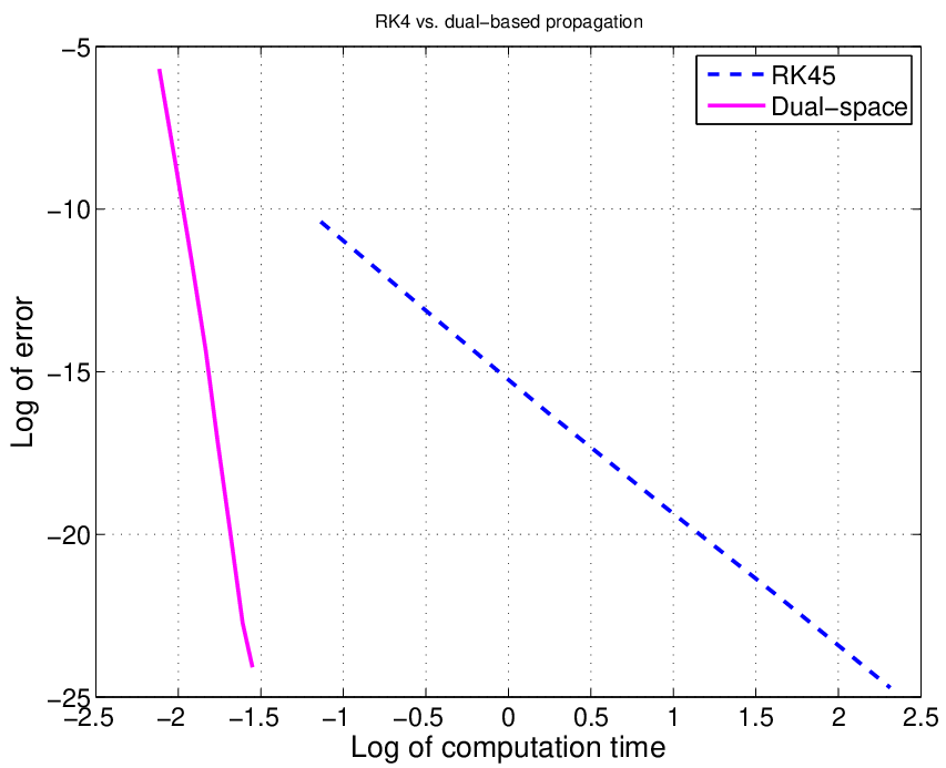
Refer to caption
Fig. 1: Approximation error versus computation time for standard (RK45) and dual-space propagation methods.

5 Conclusion

By exploiting a connection between an operator differential Riccati equation and a specific infinite dimensional optimal control problem, dynamic programming is employed to develop an evolution operator for propagating solutions of this equation. Examination of this evolution in a dual space, defined via semiconvexity and the Legendre-Fenchel transform, reveals the existence of a time indexed dual space operator that can be used to propagate the solution of the operator differential Riccati equation from any initial condition in a particular class. By demonstrating that these time indexed dual space operators inherit a semigroup property from dynamic programming, the set of such time indexed operators is shown to define a fundamental solution semigroup for the operator differential Riccati equation.

References

  • [1] J. Atwell, J. Borggaard, and B. King, Reduced order controllers for Burgers’ equation with a nonlinear observer, Int. J. Appl. Math. Comput. Sci., 11 (2001), pp. 1311–1330.
  • [2] G. Bachman and L. Narici, Functional Analysis, Dover (orig. Acad. Press, 1966), 2000.
  • [3] H. Banks and C. Wang, Optimal feedback control of infinite-dimensional parabolic evolution systems: Approximation techniques, SIAM Journal on Control and Optimization, 27 (1989), pp. 1182–1219.
  • [4] M. Bardi and I. Capuzzo-Dolcetta, Optimal control and viscosity solutions of Hamilton-Jacobi-Bellman equations, Systems & Control: Foundations & Application, Birkhauser, 1997.
  • [5] R. Bellman, Dynamic programming, Princeton University Press, 1957.
  • [6] P. Benner and H. Mena, Numerical solution of the infinite-dimensional LQR-problem and the associated differential riccati equations, MPI Magdeburg Preprint MPIMD/12-13 (August), (2012).
  • [7] A. Bensoussan, G. D. Prato, M. Delfour, and S. Mitter, Representation and control of infinite dimensional systems, Birkhaüser, second ed., 2007.
  • [8] R. Curtain and H. Zwart, An introduction to infinite-dimensional linear systems theory, vol. 21 of Texts in Applied Mathematics, Springer-Verlag, New York, 1995.
  • [9] P. Dower and W. McEneaney, A max-plus based fundamental solution for a class of infinite dimensional Riccati equations, in Proc. Joint 50t​h50^{th} IEEE Conference on Decision and Control and European Control Conference (Orlando FL, USA), 2011, pp. 615–620.
  • [10]  , A max-plus method for the optimal control of a diffusion equation, in proc. 51s​t51^{st} IEEE Conference on Decision & Control (Maui HI, USA), 2012, pp. 618–623.
  • [11]  , A max-plus dual space fundamental solution semigroup for operator differential Riccati equations, in proc., 21s​t21^{st} International Symposium on Mathematical Theory of Networks and Systems (Groningen, The Netherlands), 2014, pp. 148–153.
  • [12] J. Gibson and I. Rosen, Numerical approximation for the infinite-dimensional discrete-time optimal linear-quadratic regulator problem, SIAM Journal on Control and Optimization, 26 (1988), pp. 428–451.
  • [13] S. Görner and P. Benner, MPC for the Burgers equation based on an LQG design, Proc. Appl. Math. Mech., 6 (2006), pp. 781—782.
  • [14] R. Hagen, S. Roch, and B. Silbermann, C∗\mbox{C}^{*}-algebras and numerical analysis, vol. 236 of Pure and Applied Math., Marcel Dekker, 2001.
  • [15] E. Kreyszig, Introductory functional analysis with applications, Wiley, 1978.
  • [16] W. McEneaney, Max-plus methods for nonlinear control and estimation, Systems & Control: Foundations & Application, Birkhauser, 2006.
  • [17]  , A new fundamental solution for differential Riccati equations arising in control, Automatica, 44 (2008), pp. 920–936.
  • [18] A. Pazy, Semigroups of linear operators and applications to partial differential equations, vol. 44 of Applied Mathematical Sciences, Springer-Verlag, 1983.
  • [19] W. Ray, Real Analysis, Prentice-Hall, 1988.
  • [20] R. Rockafellar, Conjugate duality and optimization, SIAM Regional Conf. Series in Applied Math., 16 (1974).
  • [21] I. Rosen, Convergence of Galerkin approximations for operator Riccati equations - a nonlinear evolution equation approach, J. Math. Anal. Appl., 155 (1991), pp. 226–248.
  • [22] A. Taylor and D. Lay, Introduction to functional analysis, John Wiley, second ed., 1980.

Appendix A Continuous and strongly continuous operators

Some well-known facts concerning the continuity of operator-valued functions are recalled for completeness, see for example [18, 8, 7] and the references therein.

An operator-valued function ℱ:ℝ→ℒ⁡(𝒳){\mathcal{F}}:{\mathbb{R}}\rightarrow{\mathcal{L}}({\mathscr{X}}) is continuous at t0∈ℝt_{0}\in{\mathbb{R}} if given ϵ∈ℝ>0{\epsilon}\in{\mathbb{R}}_{>0} there exists an δ∈ℝ>0\delta\in{\mathbb{R}}_{>0} such that |t−t0|<δ⟹‖ℱ⁡(t)−ℱ⁡(t0)‖ℒ⁡(𝒳)<ϵ|t-t_{0}|<\delta\Longrightarrow\|{\mathcal{F}}(t)-{\mathcal{F}}(t_{0})\|_{{\mathcal{L}}({\mathscr{X}})}<{\epsilon}, in which ‖ℱ⁡(t)‖ℒ⁡(𝒳)≐sup‖x‖=1‖ℱ⁡(t)​x‖\|{\mathcal{F}}(t)\|_{{\mathcal{L}}({\mathscr{X}})}\doteq\sup_{\|x\|=1}\|{\mathcal{F}}(t)\,x\| denotes the induced operator norm of ℱ⁡(t)∈ℒ⁡(𝒳){\mathcal{F}}(t)\in{\mathcal{L}}({\mathscr{X}}), and ∥⋅∥\|\cdot\| is the norm on 𝒳{\mathscr{X}}. An operator-valued function ℱ:ℝ→ℒ⁡(𝒳){\mathcal{F}}:{\mathbb{R}}\rightarrow{\mathcal{L}}({\mathscr{X}}) is continuous on an interval I⊂ℝI\subset{\mathbb{R}} if it is continuous at every t0∈It_{0}\in I. The space of operator-valued functions C⁡(I,ℒ⁡(𝒳))C(I;{\mathcal{L}}({\mathscr{X}})) is defined as the space of all such continuous operator-valued functions defined on II.

Similarly, an operator-valued function ℱ:ℝ→ℒ⁡(𝒳){\mathcal{F}}:{\mathbb{R}}\rightarrow{\mathcal{L}}({\mathscr{X}}) is strongly continuous on an interval I⊂ℝI\subset{\mathbb{R}} if, for every x∈𝒳x\in{\mathscr{X}}, the function ℱ⁡(⋅)​x:I→𝒳{\mathcal{F}}(\cdot)\,x:I\rightarrow{\mathscr{X}} is continuous. That is, for any t0∈It_{0}\in I and x∈𝒳x\in{\mathscr{X}}, given ϵ∈ℝ>0{\epsilon}\in{\mathbb{R}}_{>0}, there exists a δ∈ℝ>0\delta\in{\mathbb{R}}_{>0} such that |t−t0|<δ⟹‖ℱ⁡(t)​x−ℱ⁡(t0)​x‖<ϵ|t-t_{0}|<\delta\Longrightarrow\|{\mathcal{F}}(t)\,x-{\mathcal{F}}(t_{0})\,x\|<{\epsilon}, in which ∥⋅∥\|\cdot\| denotes the norm on 𝒳{\mathscr{X}}. The space of strongly continuous operator-value functions C0​(I,ℒ​(𝒳))C_{0}(I;{\mathcal{L}}({\mathscr{X}})) is defined as the space of all such strongly continuous operator-valued functions defined on II.

These definitions are employed in (2.1) and (2.1).

Lemma A.31.

For any compact interval I⊂ℝI\subset{\mathbb{R}},

C⁡(I,ℒ⁡(𝒳))⊂C0​(I,ℒ⁡(𝒳))≡ℒ⁡(𝒳,C⁡(I,𝒳)),\displaystyle C(I;{\mathcal{L}}({\mathscr{X}}))\subset C_{0}(I;{\mathcal{L}}({\mathscr{X}}))\equiv{\mathcal{L}}({\mathscr{X}};C(I;{\mathscr{X}}))\,, (108)

in which ‖f‖C⁡(I,𝒳)≐supt∈I‖f⁡(t)‖\|f\|_{C(I;{\mathscr{X}})}\doteq\sup_{t\in I}\|f(t)\|.

Proof A.32.

Fix any ℱ∈C⁡(I,ℒ⁡(𝒳)){\mathcal{F}}\in C(I;{\mathcal{L}}({\mathscr{X}})), ϵ∈ℝ>0{\epsilon}\in{\mathbb{R}}_{>0}, and x∈𝒳x\in{\mathscr{X}}, ‖x‖≠0\|x\|\neq 0. Set ϵ1≐ϵ/‖x‖{\epsilon}_{1}\doteq{\epsilon}/\|x\|. As ℱ{\mathcal{F}} is continuous by definition, there exists a δ⁡(ϵ1)∈ℝ>0\delta({\epsilon}_{1})\in{\mathbb{R}}_{>0} such that |t−t0|<δ⁡(ϵ1)⟹‖ℱ⁡(t)−ℱ⁡(t0)‖ℒ⁡(𝒳)<ϵ1|t-t_{0}|<\delta({\epsilon}_{1})\Longrightarrow\|{\mathcal{F}}(t)-{\mathcal{F}}(t_{0})\|_{{\mathcal{L}}({\mathscr{X}})}<{\epsilon}_{1}. However, as ℱ⁡(t),ℱ⁡(t0)∈ℒ⁡(𝒳){\mathcal{F}}(t),\,{\mathcal{F}}(t_{0})\in{\mathcal{L}}({\mathscr{X}}), ‖ℱ⁡(t)​x−ℱ⁡(t0)​x‖≤‖ℱ⁡(t)−ℱ⁡(t0)‖𝒳​‖x‖<ϵ1|x|=ϵ\|{\mathcal{F}}(t)\,x-{\mathcal{F}}(t_{0})\,x\|\leq\|{\mathcal{F}}(t)-{\mathcal{F}}(t_{0})\|_{{\mathcal{{\mathscr{X}}}}}\,\|x\|<{\epsilon}_{1}\|x\|={\epsilon}. That is, |t−t0|≤δ⁡(ϵ/‖x‖)⇒‖ℱ⁡(t)​x−ℱ⁡(t0)​x‖<ϵ|t-t_{0}|\leq\delta({\epsilon}/\|x\|)\Rightarrow\|{\mathcal{F}}(t)\,x-{\mathcal{F}}(t_{0})\,x\|<{\epsilon}. As ϵ∈ℝ>0{\epsilon}\in{\mathbb{R}}_{>0} and x∈𝒳x\in{\mathscr{X}}, ‖x‖≠0\|x\|\neq 0, are arbitrary, it follows by definition that ℱ{\mathcal{F}} is strongly continuous. As ℱ∈C⁡(I,ℒ⁡(𝒳)){\mathcal{F}}\in C(I;{\mathcal{L}}({\mathscr{X}})) is arbitrary, the left-hand relation in (108) follows immediately.

The right-hand equivalence may be proved by showing that C0​(I,ℒ⁡(𝒳))⊆ℒ⁡(𝒳,C⁡(I,𝒳))C_{0}(I;{\mathcal{L}}({\mathscr{X}}))\subseteq{\mathcal{L}}({\mathscr{X}};C(I;{\mathscr{X}})) and ℒ⁡(𝒳,C⁡(I,𝒳))⊆C0​(I,ℒ⁡(𝒳)){\mathcal{L}}({\mathscr{X}};C(I;{\mathscr{X}}))\subseteq C_{0}(I;{\mathcal{L}}({\mathscr{X}})). To this end, first fix any ℱ∈C0​(I,ℒ⁡(𝒳)){\mathcal{F}}\in C_{0}(I;{\mathcal{L}}({\mathscr{X}})). As per [7, p.387], define f​(x)​(t)≐ℱ​(t)​xf(x)(t)\doteq{\mathcal{F}}(t)\,x, and note that ℱ{\mathcal{F}} is strongly continuous. Hence, given any x∈𝒳x\in{\mathscr{X}}, t0∈It_{0}\in I, ϵ∈ℝ>0{\epsilon}\in{\mathbb{R}}_{>0}, there exists a δ∈ℝ>0\delta\in{\mathbb{R}}_{>0} such that |t−t0|<δ⟹‖f⁡(x)​(t)−f⁡(x)​(t0)‖<ϵ|t-t_{0}|<\delta\Longrightarrow\|f(x)(t)-f(x)(t_{0})\|<{\epsilon}. That is, f⁡(x)∈C⁡(I,𝒳)f(x)\in C(I;{\mathscr{X}}) for each x∈𝒳x\in{\mathscr{X}}. Consequently, for each x∈𝒳x\in{\mathscr{X}}, the function ‖f⁡(x)​(⋅)‖:I→ℝ≥0\|f(x)(\cdot)\|:I\rightarrow{\mathbb{R}}_{\geq 0} must achieve a finite maximum Mx∈ℝ≥0M_{x}\in{\mathbb{R}}_{\geq 0} on II by the Extreme Value Theorem. That is, for each x∈𝒳x\in{\mathscr{X}}, ‖f⁡(x)​(t)‖=‖ℱ⁡(t)​x‖≤Mx<∞\|f(x)(t)\|=\|{\mathcal{F}}(t)\,x\|\leq M_{x}<\infty for all t∈It\in I. Hence, the Uniform Boundedness Theorem (e.g. [15, Theorem 4.7-3, p.249]) implies that there exists an M∈ℝ≥0M\in{\mathbb{R}}_{\geq 0} such that supt∈I‖ℱ⁡(t)‖ℒ⁡(𝒳)≤M<∞\sup_{t\in I}\|{\mathcal{F}}(t)\|_{{\mathcal{L}}({\mathscr{X}})}\leq M<\infty. Consequently,

‖f⁡(x)‖C⁡(I,𝒳)\displaystyle\|f(x)\|_{C(I;{\mathscr{X}})} ≐supt∈I‖f⁡(x)​(t)‖=supt∈I‖ℱ⁡(t)​x‖≤supt∈I‖ℱ⁡(t)‖ℒ⁡(𝒳)​‖x‖≤M​‖x‖.\displaystyle\doteq\sup_{t\in I}\|f(x)(t)\|=\sup_{t\in I}\|{\mathcal{F}}(t)\,x\|\leq\sup_{t\in I}\|{\mathcal{F}}(t)\|_{{\mathcal{L}}({\mathscr{X}})}\,\|x\|\leq M\,\|x\|\,.{}

That is f:𝒳→C⁡(I,𝒳)f:{\mathscr{X}}\rightarrow C(I;{\mathscr{X}}) is bounded. Furthermore, as f:𝒳→C⁡(I,𝒳)f:{\mathscr{X}}\rightarrow C(I;{\mathscr{X}}) satisfies by definition f⁡(x)=ℱ⁡(⋅)​xf(x)={\mathcal{F}}(\cdot)\,x for all x∈𝒳x\in{\mathscr{X}}, it is linear. Hence, f∈ℒ⁡(𝒳,C⁡(I,𝒳))f\in{\mathcal{L}}({\mathscr{X}};C(I;{\mathscr{X}})).

Conversely, select any f∈ℒ⁡(𝒳,C⁡(I,𝒳))f\in{\mathcal{L}}({\mathscr{X}};C(I;{\mathscr{X}})). By definition, there exists a K∈ℝ≥0K\in{\mathbb{R}}_{\geq 0} such that for all x∈𝒳x\in{\mathscr{X}}, supt∈I‖f⁡(x)​(t)‖=‖f⁡(x)‖C⁡(I,𝒳)≤K​‖x‖\sup_{t\in I}\|f(x)(t)\|=\|f(x)\|_{C(I;{\mathscr{X}})}\leq K\,\|x\|. Define ℱ​(t)​x≐f​(x)​(t){\mathcal{F}}(t)\,x\doteq f(x)(t), t∈It\in I. Hence, ‖ℱ⁡(t)​x‖≤K​‖x‖\|{\mathcal{F}}(t)\,x\|\leq K\,\|x\| for all x∈𝒳x\in{\mathscr{X}}, so that

ℱ⁡(t)\displaystyle{\mathcal{F}}(t) ∈ℒ⁡(𝒳)∀t∈I.\displaystyle\in{\mathcal{L}}({\mathscr{X}})\quad\quad\forall\ t\in I\,. (109)

Furthermore, as f⁡(x)∈C⁡(I,𝒳)f(x)\in C(I;{\mathscr{X}}) for every x∈𝒳x\in{\mathscr{X}}, given any x∈𝒳x\in{\mathscr{X}}, t0∈It_{0}\in I and ϵ∈ℝ>0{\epsilon}\in{\mathbb{R}}_{>0}, there exists a δ∈ℝ>0\delta\in{\mathbb{R}}_{>0} such that

|t−t0|<δ⟹\displaystyle|t-t_{0}|<\delta\quad\Longrightarrow\quad |f(x)(t)−f(x)(t0)|<ϵ⟺|ℱ(t)x−ℱ(t0)x|<ϵ.\displaystyle|f(x)(t)-f(x)(t_{0})|<{\epsilon}\quad\Longleftrightarrow\quad|{\mathcal{F}}(t)\,x-{\mathcal{F}}(t_{0})\,x|<{\epsilon}\,.{}

That is, ℱ:I→ℒ⁡(𝒳){\mathcal{F}}:I\rightarrow{\mathcal{L}}({\mathscr{X}}) is strongly continuous. Recalling (2.1) and (109), it follows that ℱ∈C0​(I,ℒ⁡(𝒳)){\mathcal{F}}\in C_{0}(I;{\mathcal{L}}({\mathscr{X}})).

In view of Lemma A.31, spaces C⁡(I,ℒ⁡(𝒳))C(I;{\mathcal{L}}({\mathscr{X}})) and C0​(I,ℒ​(𝒳))C_{0}(I;{\mathcal{L}}({\mathscr{X}})) of (2.1) and (2.1) may be equipped with the respective norms

‖ℱ‖C​{I}≐supt∈I‖ℱ⁡(t)‖ℒ⁡(𝒳),ℱ∈C⁡(I,ℒ⁡(𝒳)),‖ℱ‖C0​{I}≐sup‖x‖=1‖ℱ⁡(⋅)​x‖C⁡(I,𝒳),ℱ∈C0​(I,ℒ⁡(𝒳)).\displaystyle\begin{aligned} &\hskip-5.69054pt\|{\mathcal{F}}\|_{C\{I\}}\doteq\sup_{t\in I}\|{\mathcal{F}}(t)\|_{{\mathcal{L}}({\mathscr{X}})}\,,&&\hskip-5.69054pt{\mathcal{F}}\in C(I;{\mathcal{L}}({\mathscr{X}}))\,,\\ &\hskip-5.69054pt\|{\mathcal{F}}\|_{C_{0}\{I\}}\doteq\sup_{\|x\|=1}\|{\mathcal{F}}(\cdot)\,x\|_{C(I;{\mathscr{X}})}\,,&&\hskip-5.69054pt{\mathcal{F}}\in C_{0}(I;{\mathcal{L}}({\mathscr{X}}))\,.\end{aligned} (110)
Lemma A.33.

∥⋅∥C​{I}\|\cdot\|_{C\{I\}} may be extended to C0​(I,ℒ​(𝒳))C_{0}(I;{\mathcal{L}}({\mathscr{X}})), whereupon it is equivalent to ∥⋅∥C0​{I}\|\cdot\|_{C_{0}\{I\}}.

Proof A.34.

Fix ℱ∈C0​(I,ℒ⁡(𝒳)){\mathcal{F}}\in C_{0}(I;{\mathcal{L}}({\mathscr{X}})). By definition (110),

‖ℱ‖C0​{I}=sup‖x‖=1‖ℱ⁡(⋅)​x‖C⁡(I,𝒳)=sup‖x‖=1supt∈I‖ℱ⁡(t)​x‖\displaystyle\|{\mathcal{F}}\|_{C_{0}\{I\}}=\sup_{\|x\|=1}\|{\mathcal{F}}(\cdot)\,x\|_{C(I;{\mathscr{X}})}=\sup_{\|x\|=1}\sup_{t\in I}\|{\mathcal{F}}(t)\,x\|{}
=supt∈Isup‖x‖=1‖ℱ⁡(t)​x‖=supt∈I‖ℱ⁡(t)‖ℒ⁡(𝒳)≡‖ℱ‖C​{I}.\displaystyle=\sup_{t\in I}\sup_{\|x\|=1}\|{\mathcal{F}}(t)\,x\|=\sup_{t\in I}\|{\mathcal{F}}(t)\|_{{\mathcal{L}}({\mathscr{X}})}\equiv\|{\mathcal{F}}\|_{C\{I\}}\,.{}
Lemma A.35.

Given any closed interval I⊂ℝI\subset{\mathbb{R}}, the normed spaces

(C(I;ℒ(𝒳)),∥⋅∥C​{I}),(C0(I;ℒ(𝒳)),∥⋅∥C0​{I}),(C(I;{\mathcal{L}}({\mathscr{X}})),\,\|\cdot\|_{C\{I\}})\,,\qquad(C_{0}(I;{\mathcal{L}}({\mathscr{X}})),\,\|\cdot\|_{C_{0}\{I\}})\,,

defined via (2.1), (2.1), and (110), are Banach spaces.

Proof A.36.

The proof that (C(I;ℒ(𝒳)),∥⋅∥C​{I})(C(I;{\mathcal{L}}({\mathscr{X}})),\,\|\cdot\|_{C\{I\}}) is a Banach space follows a standard argument (for example, see the proof of [19, Theorem 4.3.2, p.115]) generalized to this setting. In particular, let {ℱn}\{{\mathcal{F}}_{n}\} denote a Cauchy sequence in C⁡(I,ℒ⁡(𝒳))C(I;{\mathcal{L}}({\mathscr{X}})). By inspection of (110), ‖ℱn​(t)−ℱm​(t)‖ℒ⁡(𝒳)≤‖ℱn−ℱm‖C​{I}\|{\mathcal{F}}_{n}(t)-{\mathcal{F}}_{m}(t)\|_{{\mathcal{L}}({\mathscr{X}})}\leq\|{\mathcal{F}}_{n}-{\mathcal{F}}_{m}\|_{C\{I\}} for any t∈It\in I, and n,m∈ℕn,m\in{\mathbb{N}}. Fixing any t∈It\in I, {ℱn​(t)}\{{\mathcal{F}}_{n}(t)\} defines a Cauchy sequence in (ℒ(𝒳),∥⋅∥ℒ⁡(𝒳))({\mathcal{L}}({\mathscr{X}}),\,\|\cdot\|_{{\mathcal{L}}({\mathscr{X}})}), which is a Banach space (see for example [15, Theorem 2.10-1, p.118]). Hence, there exists a ℱ⁡(t)∈ℒ⁡(𝒳){\mathcal{F}}(t)\in{\mathcal{L}}({\mathscr{X}}) such that ℱ⁡(t)=limn→∞ℱn​(t){\mathcal{F}}(t)=\lim_{n\rightarrow\infty}{\mathcal{F}}_{n}(t). Let {tn}n∈ℕ\{t_{n}\}_{n\in{\mathbb{N}}} denote a sequence in II such that limn→∞tn=t\lim_{n\rightarrow\infty}t_{n}=t. Fix ϵ∈ℝ>0{\epsilon}\in{\mathbb{R}}_{>0} and N∈ℕN\in{\mathbb{N}} sufficiently large such that ‖ℱN−ℱ‖C​{I}<ϵ3\|{\mathcal{F}}_{N}-{\mathcal{F}}\|_{C\{I\}}<{\textstyle{\frac{{\epsilon}}{3}}}. Hence, applying (110),

‖ℱN​(tn)−ℱ⁡(tn)‖\displaystyle\|{\mathcal{F}}_{N}(t_{n})-{\mathcal{F}}(t_{n})\| ≤ϵ3∀n∈ℕ.\displaystyle\leq{\textstyle{\frac{{\epsilon}}{3}}}\qquad\forall\ n\in{\mathbb{N}}. (111)

As ℱN∈C⁡(I,ℒ⁡(𝒳)){\mathcal{F}}_{N}\in C(I;{\mathcal{L}}({\mathscr{X}})), there exists a δ∈ℝ>0\delta\in{\mathbb{R}}_{>0} such that

|s−t|<δs∈I}\displaystyle\left.\begin{array}[]{r}|s-t|<\delta\\ \ s\in I\end{array}\right\} ⟹‖ℱN​(s)−ℱN​(t)‖ℒ⁡(𝒳)<ϵ3.\displaystyle\ \Longrightarrow\ \|{\mathcal{F}}_{N}(s)-{\mathcal{F}}_{N}(t)\|_{{\mathcal{L}}({\mathscr{X}})}<{\textstyle{\frac{{\epsilon}}{3}}}\,.

Furthermore, by definition of {tn}n∈ℕ\{t_{n}\}_{n\in{\mathbb{N}}}, there exists an M∈ℕM\in{\mathbb{N}} sufficiently large such that

n≥M\displaystyle n\geq M ⟹|tn−t|<δ.\displaystyle\quad\Longrightarrow\quad|t_{n}-t|<\delta\,. (114)

Hence, for all n≥Mn\geq M, the triangle inequality combined with (111), (A.36). and (114) implies that

‖ℱ⁡(tn)−ℱ⁡(t)‖ℒ⁡(𝒳)≤‖ℱ⁡(tn)−ℱN​(tn)‖ℒ⁡(𝒳)\displaystyle\|{\mathcal{F}}(t_{n})-{\mathcal{F}}(t)\|_{{\mathcal{L}}({\mathscr{X}})}\leq\|{\mathcal{F}}(t_{n})-{\mathcal{F}}_{N}(t_{n})\|_{{\mathcal{L}}({\mathscr{X}})}{}
+‖ℱN​(tn)−ℱN​(t)‖ℒ⁡(𝒳)+‖ℱN​(t)−ℱ⁡(t)‖ℒ⁡(𝒳)<ϵ.\displaystyle\quad+\|{\mathcal{F}}_{N}(t_{n})-{\mathcal{F}}_{N}(t)\|_{{\mathcal{L}}({\mathscr{X}})}+\|{\mathcal{F}}_{N}(t)-{\mathcal{F}}(t)\|_{{\mathcal{L}}({\mathscr{X}})}<{\epsilon}\,.{}

Hence, as ϵ∈ℝ>0{\epsilon}\in{\mathbb{R}}{>0} is arbitrary, ℱ{\mathcal{F}} must be continuous. That is, ℱ∈C⁡(I,ℒ⁡(𝒳)){\mathcal{F}}\in C(I;{\mathcal{L}}({\mathscr{X}})), which implies that (C(I;ℒ(𝒳)),∥⋅∥C​{I})(C(I;{\mathcal{L}}({\mathscr{X}})),\,\|\cdot\|_{C\{I\}}) is complete, and hence is a Banach space.

In order to prove that C0​(I,ℒ​(𝒳))C_{0}(I;{\mathcal{L}}({\mathscr{X}})) is a Banach space, recall by the right-hand equivalence of Lemma A.31 that C0​(I,ℒ⁡(𝒳))≡ℒ⁡(𝒳,ℒ⁡(I,𝒳))C_{0}(I;{\mathcal{L}}({\mathscr{X}}))\equiv{\mathcal{L}}({\mathscr{X}};{\mathcal{L}}(I;{\mathscr{X}})), where ℒ⁡(I,𝒳){\mathcal{L}}(I;{\mathscr{X}}) is equipped with the norm ‖f‖C⁡(I,𝒳)≐supt∈I‖f⁡(t)‖\|f\|_{C(I;{\mathscr{X}})}\doteq\sup_{t\in I}\|f(t)\|. Using the same argument as above, it may be shown that 𝒴≐(C(I;𝒳),∥⋅∥C⁡(I,𝒳)){\mathscr{Y}}\doteq(C(I;{\mathscr{X}}),\,\|\cdot\|_{C(I;{\mathscr{X}})}) is a Banach space. Hence, applying [15, Theorem 2.10-2, p.118], ℒ⁡(𝒳,𝒴){\mathcal{L}}({\mathscr{X}};{\mathscr{Y}}) is also a Banach space.

Appendix B Yosida approximation

The Yosida approximations [18, 7] of an unbounded densely defined operator 𝒜:dom​(𝒜)⊂𝒳→𝒳{\mathcal{A}}:{\textsf{dom}}({\mathcal{A}})\subset{\mathscr{X}}\rightarrow{\mathscr{X}} refer to a sequence {𝒜n}\{{\mathcal{A}}_{n}\}, n∈ℕn\in{\mathbb{N}}, of approximating bounded linear operators 𝒜n∈ℒ⁡(𝒳){\mathcal{A}}_{n}\in{\mathcal{L}}({\mathscr{X}}) that are strongly convergent to 𝒜{\mathcal{A}}. The following result is classical, see for example [18, 7], and is provided here for completeness.

Theorem B.37 (Yosida approximation).

Given an unbounded and densely defined operator 𝒜{\mathcal{A}} satisfying Assumption 1, there exists a sequence of operators {𝒜n}n∈ℕ⊂ℒ⁡(𝒳)\{{\mathcal{A}}_{n}\}_{n\in{\mathbb{N}}}\subset{\mathcal{L}}({\mathscr{X}}), such that the following properties hold:

  1. (i)

    the sequence {𝒜n}n∈ℕ\{{\mathcal{A}}_{n}\}_{n\in{\mathbb{N}}} is strongly convergent to 𝒜{\mathcal{A}} on 𝒳{\mathscr{X}}, i.e.

    limn→∞𝒜nx=𝒜x,∀x∈dom(𝒜); and\displaystyle\lim_{n\rightarrow\infty}{\mathcal{A}}_{n}\,x={\mathcal{A}}\,x\,,\qquad\forall\ x\in{\textsf{dom}}({\mathcal{A}});\text{ and} (115)
  2. (ii)

    there exists constants M∈ℝ≥1M\in{\mathbb{R}}_{\geq 1} and ω∈ℝ≥0\omega\in{\mathbb{R}}_{\geq 0} such that the (respectively, strongly and uniformly continuous) semigroups generated by 𝒜{\mathcal{A}} and 𝒜n{\mathcal{A}}_{n} satisfy the bound

    max⁡(‖e𝒜​t‖ℒ⁡(𝒳),‖e𝒜n​t‖ℒ⁡(𝒳))\displaystyle\max\left(\left\|e^{{\mathcal{A}}\,t}\right\|_{{\mathcal{L}}({\mathscr{X}})},\,\left\|e^{{\mathcal{A}}_{n}\,t}\right\|_{{\mathcal{L}}({\mathscr{X}})}\right) ≤M​eω​t∀t∈ℝ≥0,n∈ℕ.\displaystyle\leq M\,e^{\omega\,t}\qquad\forall\ t\in{\mathbb{R}}_{\geq 0},\,n\in{\mathbb{N}}\,. (116)

The proof of Theorem B.37 is standard, see for example [18]. It may be constructed via a sequence of lemmas. Its foundation is the resolvent ℛ𝒜:dom​(ℛ𝒜)⊂ℂ→ℒ⁡(𝒳){\mathcal{R}}_{{\mathcal{A}}}:{\textsf{dom}}({\mathcal{R}}_{\mathcal{A}})\subset{\mathbb{C}}\rightarrow{\mathcal{L}}({\mathscr{X}}) of operator 𝒜{\mathcal{A}}, which is defined by

ℛ𝒜​(λ)≐(λℐ−𝒜)−1,λ∈dom(ℛ𝒜),dom​(ℛ𝒜)≐{λ∈ℂ|λ​ℐ−𝒜 is invertible, with(λ​ℐ−𝒜)−1∈ℒ⁡(𝒳)}.\displaystyle\begin{aligned} {\mathcal{R}}_{{\mathcal{A}}}(\lambda)&\doteq(\lambda\,{\mathcal{I}}-{\mathcal{A}})^{-1}\,,\qquad\lambda\in{\textsf{dom}}({\mathcal{R}}_{\mathcal{A}})\,,\\ {\textsf{dom}}({\mathcal{R}}_{{\mathcal{A}}})&\doteq\left\{\lambda\in{\mathbb{C}}\,\left|\,\begin{array}[]{c}\text{$\lambda\,{\mathcal{I}}-{\mathcal{A}}$ is invertible, with}\\ (\lambda\,{\mathcal{I}}-{\mathcal{A}})^{-1}\in{\mathcal{L}}({\mathscr{X}})\end{array}\right.\right\}.\end{aligned} (117)

(Note that ρ⁡(𝒜)≐dom​(ℛ𝒜)⊂ℂ\rho({\mathcal{A}})\doteq{\textsf{dom}}({\mathcal{R}}_{\mathcal{A}})\subset{\mathbb{C}} is referred to as the resolvent set of 𝒜{\mathcal{A}}, while its complement σ⁡(𝒜)≐ℂ∖ρ⁡(𝒜)\sigma({\mathcal{A}})\doteq{\mathbb{C}}\setminus\rho({\mathcal{A}}) is referred to as the spectrum of 𝒜{\mathcal{A}}.)

Lemma B.38.

Given an unbounded and densely defined linear operator 𝒜{\mathcal{A}} satisfying Assumption 1, there exists M∈ℝ≥1M\in{\mathbb{R}}_{\geq 1}, ω0∈ℝ≥0\omega_{0}\in{\mathbb{R}}_{\geq 0}, and nω0≐⌈ω0⌉+1∈ℕn_{\omega_{0}}\doteq\lceil\omega_{0}\rceil+1\in{\mathbb{N}} such that

n∈ℕ≥nω0\displaystyle n\in{\mathbb{N}}_{\geq n_{\omega_{0}}} ⟹{‖ℛ𝒜​(n)‖ℒ⁡(𝒳)≤Mn−ω0,ℛ𝒜​(n)​x∈dom​(𝒜)∀x∈𝒳.\displaystyle\quad\Longrightarrow\quad\left\{\begin{aligned} &\|{\mathcal{R}}_{\mathcal{A}}(n)\|_{{\mathcal{L}}({\mathscr{X}})}\leq\frac{M}{n-\omega_{0}}\,,\\ &{\mathcal{R}}_{\mathcal{A}}(n)\,x\in{\textsf{dom}}({\mathcal{A}})\quad\forall\ x\in{\mathscr{X}}\,.\end{aligned}\right. (118)
Proof B.39.

By Assumption 1, 𝒜{\mathcal{A}} is the generator of a C0C_{0}-semigroup of bounded linear operators, with elements e𝒜​t∈ℒ⁡(𝒳)e^{{\mathcal{A}}\,t}\in{\mathcal{L}}({\mathscr{X}}) indexed by t∈ℝ≥0t\in{\mathbb{R}}_{\geq 0}. Hence, applying [18, Theorem 2.2, p.4], there exists an M∈ℝ≥1M\in{\mathbb{R}}_{\geq 1}, ω0∈ℝ≥0\omega_{0}\in{\mathbb{R}}_{\geq 0}, such that ‖e𝒜​t‖ℒ⁡(𝒳)≤M​eω0​t\|e^{{\mathcal{A}}\,t}\|_{{\mathcal{L}}({\mathscr{X}})}\leq M\,e^{\omega_{0}\,t} for all t∈ℝ≥0t\in{\mathbb{R}}_{\geq 0}. Define nω0≐⌈ω0⌉+1n_{\omega_{0}}\doteq\lceil\omega_{0}\rceil+1 as per the lemma statement. Fix any n∈ℕ≥nω0n\in{\mathbb{N}}_{\geq n_{\omega_{0}}}. The Hille-Yosida Theorem (for example, [18, Theorem 5.3, p.20]) implies that

‖ℛ𝒜​(n)‖ℒ⁡(𝒳)≤Mn−ω0,\displaystyle\|{\mathcal{R}}_{\mathcal{A}}(n)\|_{{\mathcal{L}}({\mathscr{X}})}\leq\frac{M}{n-\omega_{0}}\,, (119)

which is as per first assertion of (118). Fix any x∈𝒳x\in{\mathscr{X}}. Inequality (119) immediately implies that n​ℛ𝒜​(n)−ℐ∈ℒ⁡(𝒳)n\,{\mathcal{R}}_{\mathcal{A}}(n)-{\mathcal{I}}\in{\mathcal{L}}({\mathscr{X}}), so that ξ≐(n​ℛ𝒜​(n)−ℐ)​x∈𝒳\xi\doteq(n\,{\mathcal{R}}_{\mathcal{A}}(n)-{\mathcal{I}})\,x\in{\mathscr{X}}. However,

ξ\displaystyle\xi =(n​ℛ𝒜​(n)−ℐ)​x=[n​ℛ𝒜​(n)−(n​ℐ−𝒜)​ℛ𝒜​(n)]​x=𝒜​ℛ𝒜​(n)​x.\displaystyle=(n\,{\mathcal{R}}_{\mathcal{A}}(n)-{\mathcal{I}})\,x=\left[n\,{\mathcal{R}}_{\mathcal{A}}(n)-(n\,{\mathcal{I}}-{\mathcal{A}})\,{\mathcal{R}}_{\mathcal{A}}(n)\right]x={\mathcal{A}}\,{\mathcal{R}}_{\mathcal{A}}(n)\,x\,.{}

Consequently, as ξ∈𝒳\xi\in{\mathscr{X}}, it follows immediately that ℛ𝒜​(n)​x∈dom​(𝒜){\mathcal{R}}_{\mathcal{A}}(n)\,x\in{\textsf{dom}}({\mathcal{A}}). As n∈ℕ≥nω0n\in{\mathbb{N}}_{\geq n_{\omega_{0}}} and x∈𝒳x\in{\mathscr{X}} are both arbitrary, the proof is complete.

Lemma B.40.

Given an unbounded and densely defined linear operator 𝒜{\mathcal{A}} satisfying Assumption 1, and nω0∈ℕn_{\omega_{0}}\in{\mathbb{N}} as per Lemma B.38, the operator

𝒜n†\displaystyle{\mathcal{A}}_{n}^{\dagger} ≐n​𝒜​ℛ𝒜​(n),\displaystyle\doteq n\,{\mathcal{A}}\,{\mathcal{R}}_{\mathcal{A}}(n)\,, dom​(𝒜n†)≐𝒳,\displaystyle{\textsf{dom}}({\mathcal{A}}_{n}^{\dagger})\doteq{\mathscr{X}}\,, (120)

is well-defined for all n∈ℕ≥nω0n\in{\mathbb{N}}_{\geq n_{\omega_{0}}} and satisfies the following properties:

  1. (i)

    𝒜n†=n⁡(n​ℛ𝒜​(n)−ℐ)∈ℒ⁡(𝒳){\mathcal{A}}_{n}^{\dagger}=n\,(n\,{\mathcal{R}}_{\mathcal{A}}(n)-{\mathcal{I}})\in{\mathcal{L}}({\mathscr{X}}) for all n∈ℕ≥nω0n\in{\mathbb{N}}_{\geq n_{\omega_{0}}}; and

  2. (ii)

    limn→∞𝒜n†​x=𝒜​x\lim_{n\rightarrow\infty}{\mathcal{A}}_{n}^{\dagger}\,x={\mathcal{A}}\,x on 𝒳{\mathscr{X}} for all x∈𝒳x\in{\mathscr{X}}.

Proof B.41.

(The following proof is standard, see for example [7].) Define nω0∈ℕn_{\omega_{0}}\in{\mathbb{N}} as per Lemma B.38, and fix any n∈ℕ≥nω0n\in{\mathbb{N}}_{\geq n_{\omega_{0}}}, x∈𝒳x\in{\mathscr{X}}. Applying Lemma B.38, it is immediate from (118) that n​ℛ𝒜​(n)∈ℒ⁡(𝒳)n\,{\mathcal{R}}_{\mathcal{A}}(n)\in{\mathcal{L}}({\mathscr{X}}). Similarly, it is also immediate from (118) that ℛ𝒜​(n)​x∈dom​(𝒜){\mathcal{R}}_{\mathcal{A}}(n)\,x\in{\textsf{dom}}({\mathcal{A}}). Hence, the operator composition 𝒜​ℛ𝒜​(n){\mathcal{A}}\,{\mathcal{R}}_{\mathcal{A}}(n) in (120) is well-posed on dom​(ℛ𝒜​(n))=𝒳{\textsf{dom}}({\mathcal{R}}_{\mathcal{A}}(n))={\mathscr{X}}, which implies that 𝒜n†{\mathcal{A}}_{n}^{\dagger} as per (120) is well-defined with dom​(𝒜n†)=𝒳{\textsf{dom}}({\mathcal{A}}_{n}^{\dagger})={\mathscr{X}}. Furthermore, by definition (117) of ℛ𝒜​(n){\mathcal{R}}_{\mathcal{A}}(n),

𝒜n†​x\displaystyle{\mathcal{A}}_{n}^{\dagger}\,x =n​𝒜​ℛ𝒜​(n)​x=n​𝒜​(n​ℐ−𝒜)−1​x\displaystyle=n\,{\mathcal{A}}\,{\mathcal{R}}_{\mathcal{A}}(n)\,x=n\,{\mathcal{A}}\,(n\,{\mathcal{I}}-{\mathcal{A}})^{-1}\,x{}
=n2​(n​ℐ−𝒜)−1​x−n⁡(n​ℐ−𝒜)​(n​ℐ−𝒜)−1​x\displaystyle=n^{2}\,(n\,{\mathcal{I}}-{\mathcal{A}})^{-1}\,x-n\,(n\,{\mathcal{I}}-{\mathcal{A}})\,(n\,{\mathcal{I}}-{\mathcal{A}})^{-1}\,x{}
=n2​ℛ𝒜​(n)​x−n​ℐ​x=n⁡(n​ℛ𝒜​(n)−ℐ)​x.\displaystyle=n^{2}\,{\mathcal{R}}_{\mathcal{A}}(n)\,x-n\,{\mathcal{I}}\,x=n\,(n\,{\mathcal{R}}_{\mathcal{A}}(n)-{\mathcal{I}})\,x\,. (121)

As ℛ𝒜​(n)∈ℒ​(𝒳){\mathcal{R}}_{\mathcal{A}}(n)\in{\mathcal{L}}({\mathscr{X}}) by Lemma B.38,

‖𝒜n†‖ℒ⁡(𝒳)\displaystyle\|{\mathcal{A}}_{n}^{\dagger}\|_{{\mathcal{L}}({\mathscr{X}})} ≤n⁡(n​‖ℛ𝒜​(n)‖ℒ⁡(𝒳)+1)≤n⁡(n​Mn−ω0+1)<∞.\displaystyle\leq n\,(n\,\|{\mathcal{R}}_{\mathcal{A}}(n)\|_{{\mathcal{L}}({\mathscr{X}})}+1)\leq n\left(\frac{n\,M}{n-\omega_{0}}+1\right)<\infty\,.{}

As n∈ℕ≥nω0n\in{\mathbb{N}}_{\geq n_{\omega_{0}}} is arbitrary, it follows immediately that assertion (i) holds. In order to prove assertion (ii), fix any n∈ℕ≥nω0n\in{\mathbb{N}}_{\geq n_{\omega_{0}}}, x,ξ∈dom​(𝒜)x,\xi\in{\textsf{dom}}({\mathcal{A}}), and set y≐𝒜​xy\doteq{\mathcal{A}}\,x. Further manipulation of (121) yields

𝒜n†​x\displaystyle{\mathcal{A}}_{n}^{\dagger}\,x =n2​ℛ𝒜​(n)​x−n​ℐ​x=n​ℛ𝒜​(n)​[n​ℐ−(n​ℐ−𝒜)]​x=n​ℛ𝒜​(n)​𝒜​x,\displaystyle=n^{2}\,{\mathcal{R}}_{\mathcal{A}}(n)\,x-n\,{\mathcal{I}}\,x=n\,{\mathcal{R}}_{\mathcal{A}}(n)\left[n\,{\mathcal{I}}-(n\,{\mathcal{I}}-{\mathcal{A}})\right]x=n\,{\mathcal{R}}_{\mathcal{A}}(n)\,{\mathcal{A}}\,x\,, (122)

while

(n​ℛ𝒜​(n)−ℐ)​ξ\displaystyle(n\,{\mathcal{R}}_{\mathcal{A}}(n)-{\mathcal{I}})\,\xi =[n​ℛ𝒜​(n)−ℛ𝒜​(n)​(n​ℐ−𝒜)]​ξ=ℛ𝒜​(n)​𝒜​ξ.\displaystyle=[n\,{\mathcal{R}}_{\mathcal{A}}(n)-{\mathcal{R}}_{\mathcal{A}}(n)\,(n\,{\mathcal{I}}-{\mathcal{A}})]\,\xi={\mathcal{R}}_{\mathcal{A}}(n)\,{\mathcal{A}}\,\xi\,. (123)

Hence, writing (n​ℛ𝒜​(n)−ℐ)​y=(n​ℛ𝒜​(n)−ℐ)​ξ+(n​ℛ𝒜​(n)−ℐ)​(y−ξ)(n\,{\mathcal{R}}_{\mathcal{A}}(n)-{\mathcal{I}})\,y=(n\,{\mathcal{R}}_{\mathcal{A}}(n)-{\mathcal{I}})\,\xi+(n\,{\mathcal{R}}_{\mathcal{A}}(n)-{\mathcal{I}})\,(y-\xi),

‖(n​ℛ𝒜​(n)−ℐ)​y‖\displaystyle\|(n\,{\mathcal{R}}_{\mathcal{A}}(n)-{\mathcal{I}})\,y\| ≤‖(n​ℛ𝒜​(n)−ℐ)​ξ‖+‖(n​ℛ𝒜​(n)−ℐ)​(y−ξ)‖\displaystyle\leq\|(n\,{\mathcal{R}}_{\mathcal{A}}(n)-{\mathcal{I}})\,\xi\|+\|(n\,{\mathcal{R}}_{\mathcal{A}}(n)-{\mathcal{I}})\,(y-\xi)\|{}
=‖ℛ𝒜​(n)​𝒜​ξ‖+‖(n​ℛ𝒜​(n)−ℐ)​(y−ξ)‖\displaystyle=\|{\mathcal{R}}_{\mathcal{A}}(n)\,{\mathcal{A}}\,\xi\|+\|(n\,{\mathcal{R}}_{\mathcal{A}}(n)-{\mathcal{I}})\,(y-\xi)\|{}
≤‖ℛ𝒜​(n)‖ℒ⁡(𝒳)​‖𝒜​ξ​‖+‖n​ℛ𝒜​(n)−ℐ‖ℒ⁡(𝒳)‖​y−ξ‖\displaystyle\leq\|{\mathcal{R}}_{\mathcal{A}}(n)\|_{{\mathcal{L}}({\mathscr{X}})}\,\|{\mathcal{A}}\,\xi\|+\|n\,{\mathcal{R}}_{\mathcal{A}}(n)-{\mathcal{I}}\|_{{\mathcal{L}}({\mathscr{X}})}\,\|y-\xi\|{}
≤‖ℛ𝒜​(n)‖ℒ⁡(𝒳)​‖𝒜​ξ​‖+(n​‖ℛ𝒜​(n)‖ℒ⁡(𝒳)+1)‖​y−ξ‖\displaystyle\leq\|{\mathcal{R}}_{\mathcal{A}}(n)\|_{{\mathcal{L}}({\mathscr{X}})}\,\|{\mathcal{A}}\,\xi\|+\left(n\,\|{\mathcal{R}}_{\mathcal{A}}(n)\|_{{\mathcal{L}}({\mathscr{X}})}+1\right)\,\|y-\xi\| (124)

where the inequalities follow respectively by the triangle inequality and Lemma B.38 (i.e. that n​ℛ𝒜​(n)∈ℒ⁡(𝒳)n\,{\mathcal{R}}_{\mathcal{A}}(n)\in{\mathcal{L}}({\mathscr{X}})), while the equality follows by (123). Subtracting y=𝒜​xy={\mathcal{A}}\,x from both sides of (122), taking the norm, and applying (124) then yields

‖𝒜n†​x−𝒜​x‖\displaystyle\|{\mathcal{A}}_{n}^{\dagger}\,x-{\mathcal{A}}\,x\| =‖(n​ℛ𝒜​(n)−ℐ)​𝒜​x‖\displaystyle=\|(n\,{\mathcal{R}}_{\mathcal{A}}(n)-{\mathcal{I}})\,{\mathcal{A}}\,x\|{}
≤‖ℛ𝒜​(n)‖ℒ⁡(𝒳)​‖𝒜​ξ​‖+(n​‖ℛ𝒜​(n)‖ℒ⁡(𝒳)+1)‖​𝒜​x−ξ‖.\displaystyle\leq\|{\mathcal{R}}_{\mathcal{A}}(n)\|_{{\mathcal{L}}({\mathscr{X}})}\,\|{\mathcal{A}}\,\xi\|+(n\,\|{\mathcal{R}}_{\mathcal{A}}(n)\|_{{\mathcal{L}}({\mathscr{X}})}+1)\,\|{\mathcal{A}}\,x-\xi\|\,. (125)

As n∈ℕ≥nω0n\in{\mathbb{N}}_{\geq n_{\omega_{0}}} is arbitrary, (125) holds in particular for any n∈{ni}i∈ℕn\in\{n_{i}\}_{i\in{\mathbb{N}}}, where {ni}i∈ℕ\{n_{i}\}_{i\in{\mathbb{N}}} is any sequence in ℕ≥nω0{\mathbb{N}}_{\geq n_{\omega_{0}}} satisfying limi→∞ni=∞\lim_{i\rightarrow\infty}n_{i}=\infty. Hence,

limn→∞\displaystyle\lim_{n\rightarrow\infty} ‖𝒜n†​x−𝒜​x‖≤(limn→∞‖ℛ𝒜​(n)‖)​‖𝒜​ξ‖+(limn→∞n​‖ℛ𝒜​(n)‖ℒ⁡(𝒳)+1)​‖𝒜​x−ξ‖\displaystyle\|{\mathcal{A}}_{n}^{\dagger}\,x-{\mathcal{A}}\,x\|\leq\left(\lim_{n\rightarrow\infty}\|{\mathcal{R}}_{\mathcal{A}}(n)\|\right)\|{\mathcal{A}}\,\xi\|+\left(\lim_{n\rightarrow\infty}n\,\|{\mathcal{R}}_{\mathcal{A}}(n)\|_{{\mathcal{L}}({\mathscr{X}})}+1\right)\,\|{\mathcal{A}}\,x-\xi\|{}
≤(limn→∞Mn−ω0)​‖𝒜​ξ‖+(limn→∞n​Mn−ω0+1)​‖𝒜​x−ξ‖=M​‖𝒜​x−ξ‖,\displaystyle\leq\left(\lim_{n\rightarrow\infty}\frac{M}{n-\omega_{0}}\right)\|{\mathcal{A}}\,\xi\|+\left(\lim_{n\rightarrow\infty}\frac{n\,M}{n-\omega_{0}}+1\right)\,\|{\mathcal{A}}\,x-\xi\|=M\,\|{\mathcal{A}}\,x-\xi\|\,,{}

where the right-hand side limits follow by Lemma B.38. As ξ∈dom​(𝒜)\xi\in{\textsf{dom}}({\mathcal{A}}) is arbitrary,

limn→∞‖𝒜n†​x−𝒜​x‖\displaystyle\lim_{n\rightarrow\infty}\|{\mathcal{A}}_{n}^{\dagger}\,x-{\mathcal{A}}\,x\| ≤M⁡[infξ∈dom​(𝒜)‖𝒜​x−ξ‖]=0,\displaystyle\leq M\left[\inf_{\xi\in{\textsf{dom}}({\mathcal{A}})}\|{\mathcal{A}}\,x-\xi\|\right]=0\,,{}

where 𝒜​x∈𝒳{\mathcal{A}}\,x\in{\mathscr{X}} and dom​(𝒜){\textsf{dom}}({\mathcal{A}}) dense in 𝒳{\mathscr{X}} yields the final equality. As x∈𝒳x\in{\mathscr{X}} is arbitrary, it follows that assertion (ii) holds.

Lemma B.42.

Given an unbounded and densely defined linear operator 𝒜{\mathcal{A}} satisfying Assumption 1, there exists M∈ℝ≥1M\in{\mathbb{R}}_{\geq 1} and ω∈ℝ≥0\omega\in{\mathbb{R}}_{\geq 0} such that the operators 𝒜n†∈ℒ⁡(𝒳){\mathcal{A}}_{n}^{\dagger}\in{\mathcal{L}}({\mathscr{X}}) of (120) are well-defined for all n∈ℕ≥nωn\in{\mathbb{N}}_{\geq n_{\omega}}, nω≐⌈ω⌉+1∈ℕn_{\omega}\doteq\lceil\omega\rceil+1\in{\mathbb{N}}, with the (respectively C0C_{0}- and uniformly continuous) semigroups e𝒜​te^{{\mathcal{A}}\,t} and e𝒜n†​te^{{\mathcal{A}}_{n}^{\dagger}\,t} generated by 𝒜{\mathcal{A}} and 𝒜n†{\mathcal{A}}_{n}^{\dagger} satisfying the common bound

max⁡(‖e𝒜​t‖,‖e𝒜n†​t‖)≤M​eω​t∀t∈ℝ≥0,n∈ℕ≥nω.\displaystyle\max(\|e^{{\mathcal{A}}\,t}\|,\,\|e^{{\mathcal{A}}_{n}^{\dagger}\,t}\|)\leq M\,e^{\omega\,t}\qquad\forall\ t\in{\mathbb{R}}_{\geq 0},\,n\in{\mathbb{N}}_{\geq n_{\omega}}\,. (126)
Proof B.43.

The proof follows that provided in [7]. In particular, by Assumption 1, 𝒜{\mathcal{A}} is the generator of a C0C_{0}-semigroup of bounded linear operators, with elements e𝒜​t∈ℒ⁡(𝒳)e^{{\mathcal{A}}\,t}\in{\mathcal{L}}({\mathscr{X}}) indexed by t∈ℝ≥0t\in{\mathbb{R}}_{\geq 0}. Hence, applying [18, Theorem 2.2, p.4] (and as per the proof of Lemma B.38), there exists M∈ℝ≥1M\in{\mathbb{R}}_{\geq 1} and ω0∈ℝ≥0\omega_{0}\in{\mathbb{R}}_{\geq 0} such that

‖e𝒜​t‖\displaystyle\|e^{{\mathcal{A}}\,t}\| ≤M​eω0​t∀t∈ℝ≥0.\displaystyle\leq M\,e^{\omega_{0}\,t}\qquad\forall\ t\in{\mathbb{R}}_{\geq 0}\,. (127)

Define ω≐2​ω0∈ℝ≥0\omega\doteq 2\,\omega_{0}\in{\mathbb{R}}_{\geq 0} and nω≐⌈ω⌉+1n_{\omega}\doteq\lceil\omega\rceil+1 as per the lemma statement (see also [7, p.102]). Fix any t∈ℝ≥0t\in{\mathbb{R}}_{\geq 0} and n∈ℕ≥nωn\in{\mathbb{N}}_{\geq n_{\omega}}. Note in particular that n≥nω≥max⁡(⌈ω0⌉+1,⌈2​ω0⌉)n\geq n_{\omega}\geq\max(\lceil\omega_{0}\rceil+1,\,\lceil 2\,\omega_{0}\rceil). Hence, as n≥⌈ω0⌉+1n\geq\lceil\omega_{0}\rceil+1, assertion (i) of Lemma B.40 implies that 𝒜n†∈ℒ⁡(𝒳){\mathcal{A}}_{n}^{\dagger}\in{\mathcal{L}}({\mathscr{X}}) is well-defined by (120). Subsequently, [18, Theorem 1.2, p.2] implies that 𝒜n†{\mathcal{A}}_{n}^{\dagger} generates a uniformly continuous semigroup of bounded linear operators, each of which enjoys an explicit series representation. In particular, for the t∈ℝ≥0t\in{\mathbb{R}}_{\geq 0} fixed above,

e𝒜n†​t\displaystyle e^{{\mathcal{A}}_{n}^{\dagger}\,t} =∑k=0∞tkk!​(𝒜n†)k=e−n​t​∑k=0∞(n2​t)kk!​(ℛ𝒜​(n))k,\displaystyle=\sum_{k=0}^{\infty}\frac{t^{k}}{k!}\,({\mathcal{A}}_{n}^{\dagger})^{k}=e^{-n\,t}\sum_{k=0}^{\infty}\frac{(n^{2}\,t)^{k}}{k!}\,({\mathcal{R}}_{\mathcal{A}}(n))^{k}\,, (128)

where the second equality follows by assertion (i) of Lemma B.40 (see [7, equation (2.30), p.102]). The Hille-Yosida Theorem [18, Theorem 5.3, p.20] also implies that

‖ℛ𝒜​(n)k‖ℒ⁡(𝒳)\displaystyle\|{\mathcal{R}}_{\mathcal{A}}(n)^{k}\|_{{\mathcal{L}}({\mathscr{X}})} ≤M(n−ω0)k\displaystyle\leq\frac{M}{(n-\omega_{0})^{k}} (129)

for all k∈ℕk\in{\mathbb{N}}, where MM and ω0\omega_{0} are as per (127). Hence, returning to (128),

‖e𝒜n†​t‖ℒ⁡(𝒳)=e−n​t​‖∑k=0∞(n2​t)kk!​(ℛ𝒜​(n))k‖ℒ⁡(𝒳)≤e−n​t​∑k=0∞(n2​t)kk!​‖ℛ𝒜​(n)k‖ℒ⁡(𝒳)\displaystyle\|e^{{\mathcal{A}}_{n}^{\dagger}\,t}\|_{{\mathcal{L}}({\mathscr{X}})}=e^{-n\,t}\left\|\sum_{k=0}^{\infty}\frac{(n^{2}\,t)^{k}}{k!}\,({\mathcal{R}}_{\mathcal{A}}(n))^{k}\right\|_{{\mathcal{L}}({\mathscr{X}})}\leq e^{-n\,t}\sum_{k=0}^{\infty}\frac{(n^{2}\,t)^{k}}{k!}\,\|{\mathcal{R}}_{\mathcal{A}}(n)^{k}\|_{{\mathcal{L}}({\mathscr{X}})}{}
≤e−n​t​∑k=0∞(n2​t)kk!​M(n−ω0)k=M​e−n​t​en2​t/(n−ω0)=M​en​ω0​t/(n−ω0).\displaystyle\leq e^{-n\,t}\sum_{k=0}^{\infty}\frac{(n^{2}\,t)^{k}}{k!}\,\frac{M}{(n-\omega_{0})^{k}}=M\,e^{-n\,t}\,e^{n^{2}\,t/(n-\omega_{0})}=M\,e^{n\,\omega_{0}\,t/(n-\omega_{0})}\,. (130)

Recalling the definition of n∈ℕ≥nωn\in{\mathbb{N}}_{\geq n_{\omega}}, note that n≥2​ω0n\geq 2\,\omega_{0}. As α:[2​ω0,∞)→ℝ\alpha:[2\,\omega_{0},\infty)\rightarrow{\mathbb{R}} defined by α⁡(r)≐r​ω0/(r−ω0)\alpha(r)\doteq r\,\omega_{0}/(r-\omega_{0}) for all r≥2​ω0r\geq 2\,\omega_{0} is monotone decreasing,

n​ω0n−ω0\displaystyle\frac{n\,\omega_{0}}{n-\omega_{0}} ≤α⁡(2​ω0)=2​ω022​ω0−ω0=2​ω0=ω.\displaystyle\leq\alpha(2\,\omega_{0})=\frac{2\,\omega_{0}^{2}}{2\,\omega_{0}-\omega_{0}}=2\,\omega_{0}=\omega\,. (131)

Consequently,

‖e𝒜​t‖ℒ⁡(𝒳)\displaystyle\|e^{{\mathcal{A}}\,t}\|_{{\mathcal{L}}({\mathscr{X}})} ≤M​eω​t,‖e𝒜n†​t‖ℒ⁡(𝒳)≤M​eω​t,\displaystyle\leq M\,e^{\omega\,t}\,,\qquad\|e^{{\mathcal{A}}_{n}^{\dagger}\,t}\|_{{\mathcal{L}}({\mathscr{X}})}\leq M\,e^{\omega\,t}\,, (132)

where the first inequality follows by inspection of (127) and noting that ω0≤2​ω0=ω\omega_{0}\leq 2\,\omega_{0}=\omega, and the second inequality follows by substituting (131) in (130). As t∈ℝ≥0t\in{\mathbb{R}}_{\geq 0} and n∈ℕ≥nωn\in{\mathbb{N}}_{\geq n_{\omega}} are arbitrary, the proof is complete.

The proof of Theorem B.37 is straightforward in view of Lemmas B.40 and B.42.

Proof B.44 (Theorem B.37).

With operator 𝒜{\mathcal{A}} fixed as per the theorem statement, let nω0,nω∈ℕn_{\omega_{0}},\,n_{\omega}\in{\mathbb{N}} be defined respectively by Lemmas B.40 and Lemma B.42. Recalling the proof of the latter lemma, note in particular that nω≥nω0n_{\omega}\geq n_{\omega_{0}}. Consequently, Lemma B.40 implies that the operator 𝒜n†{\mathcal{A}}_{n}^{\dagger} of (120) is well-defined for all n∈ℕ≥nωn\in{\mathbb{N}}_{\geq n_{\omega}}. It follows immediately that the operator

𝒜n\displaystyle{\mathcal{A}}_{n} ≐𝒜n−nω+1†,\displaystyle\doteq{\mathcal{A}}_{n-n_{\omega}+1}^{\dagger}\,, dom​(𝒜n)=𝒳\displaystyle{\textsf{dom}}({\mathcal{A}}_{n})={\mathscr{X}} (133)

is well defined for every n∈ℕn\in{\mathbb{N}}. Hence, assertion (ii) of Lemma B.40 implies that assertion (i) of the hypothesis holds. Similarly, Lemma B.42 immediately implies that assertion (ii) of the hypothesis holds, thereby completing the proof.

Remark B.45.

As indicated in the statement of Theorem B.37, the operator 𝒜n{\mathcal{A}}_{n}, n∈ℕn\in{\mathbb{N}}, of (133) is referred to throughout as a Yosida approximation. Elsewhere, for example [18], this terminology is reserved for the operator 𝒜n†{\mathcal{A}}_{n}^{\dagger}, n∈ℕ≥nωn\in{\mathbb{N}}_{\geq n_{\omega}}, of (120).

Appendix C Proof of Theorem 2.9

Fix any ℳ∈Σ⁡(𝒳){\mathcal{M}}\in\Sigma({\mathscr{X}}) such that Assumption 2.8 holds, any ℳ~∈Σℳ​(𝒳){\widetilde{{\mathcal{{M}}}}}\in\Sigma_{\mathcal{M}}({\mathscr{X}}), and any n∈ℕn\in{\mathbb{N}}. Theorem 2.4 implies that there exists a τ^0∈ℝ>0\hat{\tau}_{0}\in{\mathbb{R}}_{>0} (independent of n∈ℕn\in{\mathbb{N}}), 𝒫n,𝒫~n∈C⁡([0,τ^0],Σ⁡(𝒳)){\mathcal{P}}_{n},\,{\widetilde{{\mathcal{{P}}}}}_{n}\in C([0,\hat{\tau}_{0}];\Sigma({\mathscr{X}})), and 𝒫∈C0​([0,τ^0],Σ⁡(𝒳)){\mathcal{P}}\in C_{0}([0,\hat{\tau}_{0}];\Sigma({\mathscr{X}})) such that 𝒫n{\mathcal{P}}_{n} and 𝒫~n{\widetilde{{\mathcal{{P}}}}}_{n} are unique solutions of (11) satisfying 𝒫n​(0)=ℳ{\mathcal{P}}_{n}(0)={\mathcal{M}} and 𝒫~n​(0)=ℳ~{\widetilde{{\mathcal{{P}}}}}_{n}(0)={\widetilde{{\mathcal{{M}}}}} respectively, and 𝒫{\mathcal{P}} is the unique mild solution of (1) satisfying 𝒫⁡(0)=ℳ{\mathcal{P}}(0)={\mathcal{M}}. Hence, ℰ~n∈C⁡([0,τ^0],Σ⁡(𝒳)){\widetilde{{\mathcal{{E}}}}}_{n}\in C([0,\hat{\tau}_{0}];\Sigma({\mathscr{X}})) is well defined by

ℰ~n​(t)≐𝒫~n​(t)−𝒫n​(t)\displaystyle{\widetilde{{\mathcal{{E}}}}}_{n}(t)\doteq{\widetilde{{\mathcal{{P}}}}}_{n}(t)-{\mathcal{P}}_{n}(t) (134)

for all t∈[0,τ^0]t\in[0,\hat{\tau}_{0}], where it may be noted that ℰ~n​(0)=ℳ~−ℳ{\widetilde{{\mathcal{{E}}}}}_{n}(0)={\widetilde{{\mathcal{{M}}}}}-{\mathcal{M}}, which is coercive by definition of ℳ~∈Σℳ​(𝒳){\widetilde{{\mathcal{{M}}}}}\in\Sigma_{\mathcal{M}}({\mathscr{X}}). Formally differentiating (134) and applying (11) twice (for 𝒫~n{\widetilde{{\mathcal{{P}}}}}_{n} and 𝒫n{\mathcal{P}}_{n}) yields the evolution equation

ℰ~˙n​(t)\displaystyle\dot{{\widetilde{{\mathcal{{E}}}}}}_{n}(t) =ℒ~n​(t)′​ℰ~n​(t)+ℰ~n​(t)​ℒ~n​(t),\displaystyle={\widetilde{{\mathcal{{L}}}}}_{n}(t)^{\prime}\,{\widetilde{{\mathcal{{E}}}}}_{n}(t)+{\widetilde{{\mathcal{{E}}}}}_{n}(t)\,{\widetilde{{\mathcal{{L}}}}}_{n}(t)\,, (135)

which holds for all t∈[0,τ^0]t\in[0,\hat{\tau}_{0}], with ℒ~n​(t)≐𝒜n+12​σ​σ′​(𝒫n​(t)+𝒫~n​(t)){\widetilde{{\mathcal{{L}}}}}_{n}(t)\doteq{\mathcal{A}}_{n}+{\textstyle\frac{1}{2}}\,\sigma\,\sigma^{\prime}\,({\mathcal{P}}_{n}(t)+{\widetilde{{\mathcal{{P}}}}}_{n}(t)), with 𝒜n{\mathcal{A}}_{n} denoting the Yosida approximation of 𝒜{\mathcal{A}}. In order to define the notion of solution for (135), it is also useful to consider the related operator evolution equation

𝒴~˙n​(t)\displaystyle\dot{{\widetilde{{\mathcal{{Y}}}}}}_{n}(t) =ℒ~n​(t)′​𝒴~n​(t).\displaystyle={\widetilde{{\mathcal{{L}}}}}_{n}(t)^{\prime}\,{\widetilde{{\mathcal{{Y}}}}}_{n}(t)\,. (136)

A solution of (136) on a time interval [0,T][0,T], T∈[0,τ^1]T\in[0,\hat{\tau}_{1}], is any operator-valued function 𝒴~n∈C⁡([0,T],Σ⁡(𝒳)){\widetilde{{\mathcal{{Y}}}}}_{n}\in C([0,T];\Sigma({\mathscr{X}})) satisfying

𝒴~n​(t)​x\displaystyle{\widetilde{{\mathcal{{Y}}}}}_{n}(t)\,x =e𝒜n′​t​𝒴~n​(0)​x+12​∫0te𝒜n′​(t−s)​(σ​σ′​[𝒫n​(s)+𝒫~n​(s)])′​𝒴~n​(s)​x​𝑑s\displaystyle=e^{{\mathcal{A}}_{n}^{\prime}\,t}\,{\widetilde{{\mathcal{{Y}}}}}_{n}(0)\,x+{\textstyle\frac{1}{2}}\,\int_{0}^{t}e^{{\mathcal{A}}_{n}^{\prime}\,(t-s)}\,(\sigma\,\sigma^{\prime}\,[{\mathcal{P}}_{n}(s)+{\widetilde{{\mathcal{{P}}}}}_{n}(s)])^{\prime}\,{\widetilde{{\mathcal{{Y}}}}}_{n}(s)\,x\,ds (137)

for all x∈𝒳x\in{\mathscr{X}}, t∈[0,T]t\in[0,T], where e𝒜n′⋅e^{{\mathcal{A}}_{n}^{\prime}\,\cdot} denotes the uniformly continuous semigroup generated by the Yosida approximation 𝒜n′∈ℒ⁡(𝒳){\mathcal{A}}_{n}^{\prime}\in{\mathcal{L}}({\mathscr{X}}) of 𝒜′{\mathcal{A}}^{\prime}.

Claim 1.

Given any 𝒴0∈Σ⁡(𝒳){\mathcal{Y}}_{0}\in\Sigma({\mathscr{X}}), there exists a τ1∈(0,τ^1]\tau_{1}\in(0,\hat{\tau}_{1}] such that the operator evolution equation (136) exhibit a unique solution 𝒴~n∈C⁡([0,τ1],Σ⁡(𝒳)){\widetilde{{\mathcal{{Y}}}}}_{n}\in C([0,\tau_{1}];\Sigma({\mathscr{X}})) satisfying 𝒴~n​(0)=𝒴0{\widetilde{{\mathcal{{Y}}}}}_{n}(0)={\mathcal{Y}}_{0} for all n∈ℕn\in{\mathbb{N}}.

Proof C.46 (Claim 1).

The argument largely follows that of the proof of Theorem 2.4, with the only significant departure being that it must be shown that ‖𝒫n‖C⁡[0,τ^1]\|{\mathcal{P}}_{n}\|_{C[0,\hat{\tau}_{1}]} (and ‖𝒫~n‖C⁡[0,τ^1]\|{\widetilde{{\mathcal{{P}}}}}_{n}\|_{C[0,\hat{\tau}_{1}]}) can be bounded above uniformly with respect to n∈ℕn\in{\mathbb{N}}. To this end, recall that 𝒫n∈C⁡([0,τ^1],Σ⁡(𝒳))⊂ℒ⁡(𝒳,C⁡([0,τ^1],𝒳)){\mathcal{P}}_{n}\in C([0,\hat{\tau}_{1}];\Sigma({\mathscr{X}}))\subset{\mathcal{L}}({\mathscr{X}};C([0,\hat{\tau}_{1}];{\mathscr{X}})) by Lemma A.31. Furthermore, Theorem 2.4 and the triangle inequality imply that

0\displaystyle 0 =limn→∞‖𝒫n​(⋅)​x−𝒫⁡(⋅)​x‖C⁡([0,t],𝒳)≥limn→∞|‖𝒫n​(⋅)​x‖C⁡([0,t],𝒳)−‖𝒫⁡(⋅)​x‖C⁡([0,t],𝒳)|\displaystyle=\lim_{n\rightarrow\infty}\left\|{\mathcal{P}}_{n}(\cdot)\,x-{\mathcal{P}}(\cdot)\,x\right\|_{C([0,t];{\mathscr{X}})}\geq\lim_{n\rightarrow\infty}\left|\left\|{\mathcal{P}}_{n}(\cdot)\,x\right\|_{C([0,t];{\mathscr{X}})}-\left\|{\mathcal{P}}(\cdot)\,x\right\|_{C([0,t];{\mathscr{X}})}\right|{}

for all x∈𝒳x\in{\mathscr{X}}. That is, the sequence {pn}n∈ℕ⊂ℝ≥0\{p_{n}\}_{n\in{\mathbb{N}}}\subset{\mathbb{R}}_{\geq 0}, pn≐‖𝒫n​(⋅)​x‖C⁡([0,t],𝒳)p_{n}\doteq\left\|{\mathcal{P}}_{n}(\cdot)\,x\right\|_{C([0,t];{\mathscr{X}})}, is convergent, and hence bounded. In particular, for each x∈𝒳x\in{\mathscr{X}}, there exists an Mx∈ℝ≥0M_{x}\in{\mathbb{R}}_{\geq 0} (independent of n∈ℕn\in{\mathbb{N}}) such that ‖𝒫n​(⋅)​x‖C⁡([0,t],𝒳)≤Mx<∞\|{\mathcal{P}}_{n}(\cdot)\,x\|_{C([0,t];{\mathscr{X}})}\leq M_{x}<\infty for all n∈ℕn\in{\mathbb{N}}. Consequently, as 𝒫n​(⋅)=𝒫n∈ℒ⁡(𝒳,C⁡([0,τ^1],𝒳)){\mathcal{P}}_{n}(\cdot)={\mathcal{P}}_{n}\in{\mathcal{L}}({\mathscr{X}};C([0,\hat{\tau}_{1}];{\mathscr{X}})) for all n∈ℕn\in{\mathbb{N}}, the Uniform Boundedness Theorem (for example [15, Theorem 4.7-3, p.249]) implies that there exists an M∈ℝ≥0M\in{\mathbb{R}}_{\geq 0} such that ‖𝒫n‖ℒ⁡(𝒳,C⁡([0,τ^1],𝒳))≤M<∞\|{\mathcal{P}}_{n}\|_{{\mathcal{L}}({\mathscr{X}};C([0,\hat{\tau}_{1}];{\mathscr{X}}))}\leq M<\infty for all n∈ℕn\in{\mathbb{N}}. Hence, Lemma A.33 implies that ‖𝒫n‖C⁡[0,τ^1]\|{\mathcal{P}}_{n}\|_{C[0,\hat{\tau}_{1}]} is indeed uniformly bounded as required, with

supn∈ℕ‖𝒫n‖C⁡[0,τ^1]\displaystyle\sup_{n\in{\mathbb{N}}}\|{\mathcal{P}}_{n}\|_{C[0,\hat{\tau}_{1}]} ≤M<∞.\displaystyle\leq M<\infty\,.{}

With this bound in place (along with the corresponding uniform bound for ‖𝒫~n‖C⁡[0,τ^1]\|{\widetilde{{\mathcal{{P}}}}}_{n}\|_{C[0,\hat{\tau}_{1}]}), the proof proceeds as per Theorem 2.4, with the details omitted for brevity.

Existence of a unique solution 𝒴~n{\widetilde{{\mathcal{{Y}}}}}_{n} of (136) on [0,τ1][0,\tau_{1}] as per Claim 1 implies the existence of an evolution operator that propagates 𝒴~n{\widetilde{{\mathcal{{Y}}}}}_{n} forward in time. In particular, it defines 𝒰~n:Δτ1→Σ⁡(𝒳){\widetilde{{\mathcal{{U}}}}}_{n}:\Delta_{\tau_{1}}\rightarrow\Sigma({\mathscr{X}}), Δτ1≐{(t,s)∈ℝ2|t∈[0,τ1],s∈[0,t]}\Delta_{\tau_{1}}\doteq\left\{(t,s)\in{\mathbb{R}}^{2}\,\big|\,t\in[0,\tau_{1}],\ s\in[0,t]\right\}, via

𝒰~n​(t,s)​𝒴~n​(s)​x=𝒴~n​(t)​x,\displaystyle{\widetilde{{\mathcal{{U}}}}}_{n}(t,s)\,{\widetilde{{\mathcal{{Y}}}}}_{n}(s)\,x={\widetilde{{\mathcal{{Y}}}}}_{n}(t)\,x\,, (138)

for all x∈𝒳x\in{\mathscr{X}}, (t,s)∈Δτ1(t,s)\in\Delta_{\tau_{1}}. This evolution operator 𝒰~n{\widetilde{{\mathcal{{U}}}}}_{n} satisfy a catalog of properties, see [18, Theorem 5.2, p.128] or [7, Proposition 3.6, p.138]. A subset of these is summarized as follows:

  1. (i)

    𝒰~n∈C⁡(Δτ1,ℒ⁡(𝒳)){\widetilde{{\mathcal{{U}}}}}_{n}\in C(\Delta_{\tau_{1}};{\mathcal{L}}({\mathscr{X}}));

  2. (ii)

    𝒰~n​(t,t)=ℐ{\widetilde{{\mathcal{{U}}}}}_{n}(t,t)={\mathcal{I}}, 𝒰~n​(t,s)=𝒰~n​(t,r)​𝒰~n​(r,s){\widetilde{{\mathcal{{U}}}}}_{n}(t,s)={\widetilde{{\mathcal{{U}}}}}_{n}(t,r)\,{\widetilde{{\mathcal{{U}}}}}_{n}(r,s) for all (r,s),(s,t)∈Δτ1(r,s),(s,t)\in\Delta_{\tau_{1}}; and

  3. (iii)

    𝒰~n{\widetilde{{\mathcal{{U}}}}}_{n} is differentiable, with ∂∂s​𝒰~n​(t,s)=−𝒰~n​(t,s)​ℒ~n​(s)′{\textstyle{{\frac{\partial{}}{\partial{s}}}}}\,{\widetilde{{\mathcal{{U}}}}}_{n}(t,s)=-{\widetilde{{\mathcal{{U}}}}}_{n}(t,s)\,{\widetilde{{\mathcal{{L}}}}}_{n}(s)^{\prime} for all (t,s)∈Δτ1(t,s)\in\Delta_{\tau_{1}}.

(Where ℒ~n​(t)=ℒ~n∈ℒ⁡(𝒳){\widetilde{{\mathcal{{L}}}}}_{n}(t)={\widetilde{{\mathcal{{L}}}}}_{n}\in{\mathcal{L}}({\mathscr{X}}) is independent of tt, the resulting evolution operator 𝒰~n​(t,s)=𝒰~n​(t−s){\widetilde{{\mathcal{{U}}}}}_{n}(t,s)={\widetilde{{\mathcal{{U}}}}}_{n}(t-s) defined by (138) simplifies to the element e(ℒ~n)′​(t−s)∈ℒ⁡(𝒳)e^{({\widetilde{{\mathcal{{L}}}}}_{n})^{\prime}\,(t-s)}\in{\mathcal{L}}({\mathscr{X}}) of the uniformly continuous semigroup generated by ℒ~n′{\widetilde{{\mathcal{{L}}}}}_{n}^{\prime}.)

Evolution operator 𝒰~n{\widetilde{{\mathcal{{U}}}}}_{n} facilitates the definition of the notion of solution for the evolution equation (135). In particular, a solution of (135) on a time interval [0,T][0,T], T∈[0,τ1]T\in[0,\tau_{1}], is any operator-valued function ℰ~n∈C⁡([0,T],Σ⁡(𝒳)){\widetilde{{\mathcal{{E}}}}}_{n}\in C([0,T];\Sigma({\mathscr{X}})) satisfying

ℰ~n​(t)​x\displaystyle{\widetilde{{\mathcal{{E}}}}}_{n}(t)\,x =𝒰~n​(t,0)​ℰ~n​(0)​𝒰~n​(t,0)′​x\displaystyle={\widetilde{{\mathcal{{U}}}}}_{n}(t,0)\,{\widetilde{{\mathcal{{E}}}}}_{n}(0)\,{\widetilde{{\mathcal{{U}}}}}_{n}(t,0)^{\prime}\,x (139)

for all x∈𝒳x\in{\mathscr{X}}, t∈[0,T]t\in[0,T]. (See also Appendix D.) Recalling the definition (134) of ℰ~n{\widetilde{{\mathcal{{E}}}}}_{n}, its required initialization ℰ~n​(0)=ℳ~−ℳ{\widetilde{{\mathcal{{E}}}}}_{n}(0)={\widetilde{{\mathcal{{M}}}}}-{\mathcal{M}} is coercive by definition of ℳ~∈Σℳ​(𝒳){\widetilde{{\mathcal{{M}}}}}\in\Sigma_{\mathcal{M}}({\mathscr{X}}). Furthermore, 𝒫⁡(t)−ℳ{\mathcal{P}}(t)-{\mathcal{M}} is coercive for all t∈(0,τ1]t\in(0,\tau_{1}] by Assumption 2.8. That is, there exists ϵ0∈ℝ>0{\epsilon}_{0}\in{\mathbb{R}}_{>0} and ϵ1:[0,τ1]→ℝ≥0{\epsilon}_{1}:[0,\tau_{1}]\rightarrow{\mathbb{R}}_{\geq 0}, satisfying ϵ1​(0)=0{\epsilon}_{1}(0)=0 and ϵ1​(s)>0{\epsilon}_{1}(s)>0 for all s∈(0,τ1]s\in(0,\tau_{1}], such that

⟨x,(ℳ~−ℳ)​x⟩≥ϵ0​‖x‖2,⟨x,(𝒫⁡(t)−ℳ)​x⟩≥ϵ1​(t)​‖x‖2\displaystyle\langle x,\,({\widetilde{{\mathcal{{M}}}}}-{\mathcal{M}})\,x\rangle\geq{\epsilon}_{0}\,\|x\|^{2}\,,\qquad\langle x,\,({\mathcal{P}}(t)-{\mathcal{M}})\,x\rangle\geq{\epsilon}_{1}(t)\,\|x\|^{2} (140)

for all x∈𝒳x\in{\mathscr{X}} and t∈[0,τ1]t\in[0,\tau_{1}]. Note in particular that ϵ1{\epsilon}_{1} is independent of n∈ℕn\in{\mathbb{N}}. Hence, recalling (134) and (139),

⟨x,\displaystyle\langle x,\, (𝒫~n(t)−ℳ)x⟩=⟨x,ℰ~n(t)x⟩+⟨x,(𝒫n(t)−𝒫(t))x⟩+⟨x,(𝒫(t)−ℳ)x⟩\displaystyle({\widetilde{{\mathcal{{P}}}}}_{n}(t)-{\mathcal{M}})\,x\rangle=\langle x,\,{\widetilde{{\mathcal{{E}}}}}_{n}(t)\,x\rangle+\langle x,\,({\mathcal{P}}_{n}(t)-{\mathcal{P}}(t))\,x\rangle+\langle x,\,({\mathcal{P}}(t)-{\mathcal{M}})\,x\rangle{}
=⟨𝒰~n​(t,0)′​x,(ℳ~−ℳ)​𝒰~n​(t,0)′​x⟩+⟨x,(𝒫n​(t)−𝒫⁡(t))​x⟩+⟨x,(𝒫⁡(t)−ℳ)​x⟩\displaystyle=\langle{\widetilde{{\mathcal{{U}}}}}_{n}(t,0)^{\prime}\,x,\,({\widetilde{{\mathcal{{M}}}}}-{\mathcal{M}})\,{\widetilde{{\mathcal{{U}}}}}_{n}(t,0)^{\prime}\,x\rangle+\langle x,\,({\mathcal{P}}_{n}(t)-{\mathcal{P}}(t))\,x\rangle+\langle x,\,({\mathcal{P}}(t)-{\mathcal{M}})\,x\rangle{}
≥ϵ0​‖𝒰~n​(t,0)′​x‖2−‖x‖​sups∈[0,t]‖𝒫n​(s)​x−𝒫​x​‖+ϵ1​(t)‖​x‖2\displaystyle\geq{\epsilon}_{0}\,\|{\widetilde{{\mathcal{{U}}}}}_{n}(t,0)^{\prime}\,x\|^{2}-\|x\|\,\sup_{s\in[0,t]}\|{\mathcal{P}}_{n}(s)\,x-{\mathcal{P}}\,x\|+{\epsilon}_{1}(t)\,\|x\|^{2}{}
≥ϵ1​(t)​‖x‖2−‖x‖​‖𝒫n​(⋅)​x−𝒫​x‖C⁡([0,t],𝒳),\displaystyle\geq{\epsilon}_{1}(t)\,\|x\|^{2}-\|x\|\,\|{\mathcal{P}}_{n}(\cdot)\,x-{\mathcal{P}}\,x\|_{C([0,t];{\mathscr{X}})}\,,{}

where the first inequality follows by (140) and Cauchy-Schwartz, and the second inequality follows by positivity of ϵ0{\epsilon}_{0}. Hence, taking the limit as n→∞n\rightarrow\infty, the limit relationship (14) of Theorem 2.4 implies that

⟨x,(𝒫~​(t)−ℳ)​x⟩\displaystyle\langle x,\,({\widetilde{{\mathcal{{P}}}}}(t)-{\mathcal{M}})\,x\rangle ≥ϵ1​(t)​‖x‖2\displaystyle\geq{\epsilon}_{1}(t)\,\|x\|^{2} (141)

for all x∈𝒳x\in{\mathscr{X}}, t∈[0,τ1]t\in[0,\tau_{1}], where ϵ1​(0)=0{\epsilon}_{1}(0)=0 and ϵ1​(t)>0{\epsilon}_{1}(t)>0 for all t∈(0,τ1]t\in(0,\tau_{1}]. That is, 𝒫~∈C⁡([0,τ1],Σ⁡(𝒳))∩C⁡((0,τ1],Σℳ​(𝒳)){\widetilde{{\mathcal{{P}}}}}\in C([0,\tau_{1}];\Sigma({\mathscr{X}}))\cap C((0,\tau_{1}];\Sigma_{\mathcal{M}}({\mathscr{X}})), as required. □\square

Appendix D Integral forms of operator differential equations

The notion of a mild solution of an operator differential equation is defined with respect to the corresponding operator integral equation, see for example (9), (23), (24), (32), (137), (139), etc. In each case, the integral equation is derived formally from the operator differential equation. Two example derivations are included here.

(i) Operator differential Riccati equation (1). For convenience, let Σ𝒜​(𝒳)≐{𝒫∈Σ⁡(𝒳)|𝒫​x∈dom​(𝒜)​∀x∈dom​(𝒜)}\Sigma^{\mathcal{A}}({\mathscr{X}})\doteq\{{\mathcal{P}}\in\Sigma({\mathscr{X}})\,\bigl|\,{\mathcal{P}}\,x\in{\textsf{dom}}({\mathcal{A}})\ \forall\ x\in{\textsf{dom}}({\mathcal{A}})\}. Given some horizon t∈ℝ>0t\in{\mathbb{R}}_{>0}, let 𝒫∈C01​([0,t],Σ𝒜​(𝒳)){\mathcal{P}}\in C_{0}^{1}([0,t];\Sigma^{\mathcal{A}}({\mathscr{X}})) denote a (strict) solution of the operator differential Riccati equation (9), where C01​([0,t],Σ𝒜​(𝒳))C_{0}^{1}([0,t];\Sigma^{\mathcal{A}}({\mathscr{X}})) denotes the corresponding space of strongly Frechet differentiable operator-valued functions defined on [0,t][0,t]. Define πt:[0,t]→ℒ⁡(𝒳)\pi_{t}:[0,t]\rightarrow{\mathcal{L}}({\mathscr{X}}) by πt​(s)​x≐e𝒜′​(t−s)​𝒫​(s)​e𝒜⁡(t−s)​x\pi_{t}(s)\,x\doteq e^{{\mathcal{A}}^{\prime}\,(t-s)}\,{\mathcal{P}}(s)\,e^{{\mathcal{A}}\,(t-s)}\,x, s∈[0,t]s\in[0,t], x∈𝒳x\in{\mathscr{X}}, and note that πt​(0)​x=e𝒜′​t​𝒫​(0)​e𝒜​t\pi_{t}(0)\,x=e^{{\mathcal{A}}^{\prime}\,t}\,{\mathcal{P}}(0)\,e^{{\mathcal{A}}\,t}, πt​(t)​x=𝒫⁡(t)​x\pi_{t}(t)\,x={\mathcal{P}}(t)\,x, and π⁡(⋅)​x\pi(\cdot)\,x is Fréchet differentiable. In particular, recalling [18, Theorem 2.4, p.4], the chain rule for Fréchet differentiation, and (1),

dd​s​[πt​(s)​x]\displaystyle{\textstyle{{\frac{d{}}{d{s}}}}}[\pi_{t}(s)\,x] =e𝒜′​(t−s)​[−𝒜′​𝒫​(s)+𝒫˙​(s)+𝒫⁡(s)​𝒜]​e𝒜⁡(t−s)​x\displaystyle=e^{{\mathcal{A}}^{\prime}\,(t-s)}\left[-{\mathcal{A}}^{\prime}\,{\mathcal{P}}(s)+{\dot{{\mathcal{P}}}}(s)+{\mathcal{P}}(s)\,{\mathcal{A}}\right]e^{{\mathcal{A}}\,(t-s)}\,x{}
=e𝒜′​(t−s)​[𝒫⁡(s)​σ​σ′​𝒫​(s)+𝒞]​e𝒜⁡(t−s)​x.\displaystyle=e^{{\mathcal{A}}^{\prime}\,(t-s)}\left[{\mathcal{P}}(s)\,\sigma\,\sigma^{\prime}\,{\mathcal{P}}(s)+{\mathcal{C}}\right]e^{{\mathcal{A}}\,(t-s)}\,x\,.{}

Hence, integration yields that

𝒫⁡(t)​x\displaystyle{\mathcal{P}}(t)\,x =πt​(t)​x=πt​(0)​x+∫0tdd​s​[πt​(s)​x]​𝑑s\displaystyle=\pi_{t}(t)\,x=\pi_{t}(0)\,x+\int_{0}^{t}{\textstyle{{\frac{d{}}{d{s}}}}}[\pi_{t}(s)\,x]\,ds{}
=e𝒜′​t​𝒫​(0)​e𝒜​t​x+∫0te𝒜′​s​[𝒫⁡(s)​σ​σ′​𝒫​(s)+𝒞]​e𝒜⁡(t−s)​x​𝑑s=γ⁡(𝒫)​(t)​x,\displaystyle=e^{{\mathcal{A}}^{\prime}\,t}\,{\mathcal{P}}(0)\,e^{{\mathcal{A}}\,t}\,x+\int_{0}^{t}e^{{\mathcal{A}}^{\prime}\,s}\left[{\mathcal{P}}(s)\,\sigma\,\sigma^{\prime}\,{\mathcal{P}}(s)+{\mathcal{C}}\right]e^{{\mathcal{A}}\,(t-s)}\,x\,ds=\gamma({\mathcal{P}})(t)\,x\,,{}

which is the integral form (9) of the operator differential Riccati equation (1).

(ii) Operator evolution equation (135). Given a time horizon t∈ℝ>0t\in{\mathbb{R}}_{>0}, let ℰ~n∈C1​([0,t],Σ⁡(𝒳)){\widetilde{{\mathcal{{E}}}}}_{n}\in C^{1}([0,t];\Sigma({\mathscr{X}})) denote a (strict) solution of the operator evolution equation (135), where C1​([0,t],Σ⁡(𝒳))C^{1}([0,t];\Sigma({\mathscr{X}})) denotes the corresponding space of uniformly Fréchet differentiable operator-valued functions defined on [0,t][0,t]. Define πt:[0,t]→ℒ⁡(𝒳)\pi_{t}:[0,t]\rightarrow{\mathcal{L}}({\mathscr{X}}) by πt​(s)≐𝒰~n​(t,s)​ℰ~n​(s)​𝒰~n​(t,s)′\pi_{t}(s)\doteq{\widetilde{{\mathcal{{U}}}}}_{n}(t,s)\,{\widetilde{{\mathcal{{E}}}}}_{n}(s)\,{\widetilde{{\mathcal{{U}}}}}_{n}(t,s)^{\prime} where the evolution operator 𝒰~n{\widetilde{{\mathcal{{U}}}}}_{n} is as per (138), and note that πt​(0)=𝒰~n​(t,0)​ℰ~n​(0)​𝒰~n​(t,0)′\pi_{t}(0)={\widetilde{{\mathcal{{U}}}}}_{n}(t,0)\,{\widetilde{{\mathcal{{E}}}}}_{n}(0)\,{\widetilde{{\mathcal{{U}}}}}_{n}(t,0)^{\prime}, πt​(t)=ℰ~n​(t)\pi_{t}(t)={\widetilde{{\mathcal{{E}}}}}_{n}(t), and πt​(⋅)\pi_{t}(\cdot) is Fréchet differentiable. In particular, recalling property (iii) of 𝒰~{\widetilde{{\mathcal{{U}}}}} as set out in Appendix C (or [18, Theorem 5.2, p.128]), the chain rule for Fréchet differentiation, and (135),

dd​s​[πt​(s)]\displaystyle{\textstyle{{\frac{d{}}{d{s}}}}}[\pi_{t}(s)] =𝒰~n​(t,s)​[−ℒ~n​(s)′​ℰ~n​(s)+ℰ~˙n​(s)−ℰ~n​(s)​ℒ~n​(s)]​𝒰~n​(t,s)′=0.\displaystyle={\widetilde{{\mathcal{{U}}}}}_{n}(t,s)\left[-{\widetilde{{\mathcal{{L}}}}}_{n}(s)^{\prime}\,{\widetilde{{\mathcal{{E}}}}}_{n}(s)+\dot{{\widetilde{{\mathcal{{E}}}}}}_{n}(s)-{\widetilde{{\mathcal{{E}}}}}_{n}(s)\,{\widetilde{{\mathcal{{L}}}}}_{n}(s)\right]{\widetilde{{\mathcal{{U}}}}}_{n}(t,s)^{\prime}=0\,.{}

Hence, integration yields that

ℰ~n​(t)=πt​(t)\displaystyle{\widetilde{{\mathcal{{E}}}}}_{n}(t)=\pi_{t}(t) =πt​(0)=𝒰~n​(t,0)​ℰ~n​(0)​𝒰~n​(t,0)′,\displaystyle=\pi_{t}(0)={\widetilde{{\mathcal{{U}}}}}_{n}(t,0)\,{\widetilde{{\mathcal{{E}}}}}_{n}(0)\,{\widetilde{{\mathcal{{U}}}}}_{n}(t,0)^{\prime}\,,{}

which yields the integral form (139) of the operator evolution equation (135).

Appendix E Quadratic functionals

Lemma E.47.

Given any ℱ∈Σ⁡(𝒳){\mathcal{F}}\in\Sigma({\mathscr{X}}), the quadratic functional f:𝒳→ℝf:{\mathscr{X}}\rightarrow{\mathbb{R}} defined by f⁡(x)≐12​⟨x,ℱ​x⟩f(x)\doteq{\textstyle\frac{1}{2}}\langle x,\,{\mathcal{F}}\,x\rangle, x∈𝒳x\in{\mathscr{X}}, satisfies the following properties: (i) ff is closed; and (ii) ff is convex if and only if ff is nonnegative.

Proof E.48.

(i) Fix any x∈𝒳x\in{\mathscr{X}}, δ∈(0,1]\delta\in(0,1], and any h∈𝒳h\in{\mathscr{X}} such that ‖h−x‖≤δ\|h-x\|\leq\delta.

|f⁡(x+h)−f⁡(x)|\displaystyle\left|f(x+h)-f(x)\right| ≤12​|⟨h,(ℱ+ℱ′)​x⟩|+12​|⟨h,ℱ​h⟩|\displaystyle\leq{\textstyle\frac{1}{2}}\left|\left\langle h,\,\left({\mathcal{F}}+{\mathcal{F}}^{\prime}\right)\,x\right\rangle\right|+{\textstyle\frac{1}{2}}\left|\langle h,\,{\mathcal{F}}\,h\rangle\right|{}
≤12​‖h‖​(‖(ℱ+ℱ′)​x‖+‖ℱ​h‖)≤K​‖h‖\displaystyle\leq{\textstyle\frac{1}{2}}\|h\|\left(\left\|\left({\mathcal{F}}+{\mathcal{F}}^{\prime}\right)x\right\|+\|{\mathcal{F}}\,h\|\right)\leq K\,\|h\|{}

for some K∈ℝ>0K\in{\mathbb{R}}_{>0}, where the inequalities follow respectively by the triangle inequality, Cauchy-Schwartz, and boundedness of ℱ{\mathcal{F}}. Hence, ff is continuous everywhere on 𝒳{\mathscr{X}}, and hence closed.

(ii) Given α∈[0,1]\alpha\in[0,1] and applying the definition of the quadratic functional ff, define the functional Δα:𝒳×𝒳→ℝ\Delta_{\alpha}:{\mathscr{X}}\times{\mathscr{X}}\rightarrow{\mathbb{R}} by

Δα​(x,ξ)\displaystyle\Delta_{\alpha}(x,\xi) ≐α​f​(x)+(1−α)​f​(ξ)−f⁡(α​x+(1−α)​ξ)\displaystyle\doteq\alpha f(x)+(1-\alpha)f(\xi)-f\left(\alpha\,x+(1-\alpha)\,\xi\right){}
=α⁡(1−α)​(⟨x,ℱ​x⟩+⟨ξ,ℱ​ξ⟩−⟨x,ℱ​ξ⟩−⟨ξ,ℱ​x⟩)\displaystyle=\alpha(1-\alpha)\left(\langle x,\,{\mathcal{F}}\,x\rangle+\langle\xi,\,{\mathcal{F}}\,\xi\rangle-\langle x,\,{\mathcal{F}}\,\xi\rangle-\langle\xi,\,{\mathcal{F}}\,x\rangle\right){}
=α⁡(1−α)​⟨x−ξ,ℱ⁡(x−ξ)⟩=α⁡(1−α)​f​(x−ξ),\displaystyle=\alpha(1-\alpha)\,\langle x-\xi,\,{\mathcal{F}}\left(x-\xi\right)\rangle=\alpha(1-\alpha)\,f(x-\xi)\,,{}

where linearity of ℱ{\mathcal{F}} and properties of the inner product have been used. Supposing that ff is nonnegative, Δα​(x,ξ)≥0\Delta_{\alpha}(x,\xi)\geq 0 for all x,ξ∈𝒳x,\,\xi\in{\mathscr{X}}. That is, ff is convex. Conversely, if ff is convex, then it follows by inspection that ff must be nonnegative.

Lemma E.49.

Given any ℱ:𝒳→𝒳{\mathcal{F}}:{\mathscr{X}}\rightarrow{\mathscr{X}}, ξ∈𝒳\xi\in{\mathscr{X}}, suppose that the quadratic functional f:𝒳→ℝf:{\mathscr{X}}\rightarrow{\mathbb{R}} defined by f⁡(x)≐12​⟨x,ℱ​x⟩+⟨x,ξ⟩f(x)\doteq{\textstyle\frac{1}{2}}\langle x,\,{\mathcal{F}}\,x\rangle+\langle x,\,\xi\rangle, x∈𝒳x\in{\mathscr{X}}, satisfies the property that supx∈𝒳f⁡(x)<∞\sup_{x\in{\mathscr{X}}}f(x)<\infty. Then, the following properties hold:

  1. (i)

    ℱ{\mathcal{F}} is non-positive;

  2. (ii)

    the Moore-Penrose inverse ℱ+{\mathcal{F}}^{+} of ℱ{\mathcal{F}} exists; and

  3. (iii)

    there exists an x∗∈𝒳x^{*}\in{\mathscr{X}} such that

    f⁡(x∗)\displaystyle f(x^{*}) =supx∈𝒳f⁡(x)=−12​⟨ξ,ℱ+​ξ⟩,wherex∗=−ℱ+​ξ.\displaystyle=\sup_{x\in{\mathscr{X}}}f(x)=-{\textstyle\frac{1}{2}}\langle\xi,\,{\mathcal{F}}^{+}\,\xi\rangle\,,\quad\text{where}\quad x^{*}=-{\mathcal{F}}^{+}\,\xi\,. (142)
Proof E.50.

Assume that supx∈𝒳f⁡(x)<∞\sup_{x\in{\mathscr{X}}}f(x)<\infty. Fix ξ∈𝒳\xi\in{\mathscr{X}}.

(i) Suppose that ℱ{\mathcal{F}} is positive. Given ϵ∈ℝ>0{\epsilon}\in{\mathbb{R}}_{>0}, there exists an x¯∈𝒳\bar{x}\in{\mathscr{X}} such that ϕξ​(x¯)>ϵ\phi_{\xi}(\bar{x})>{\epsilon}, where ϕξ:𝒳→ℝ\phi_{\xi}:{\mathscr{X}}\rightarrow{\mathbb{R}} is defined by

ϕξ​(x¯)\displaystyle\phi_{\xi}(\bar{x}) ≐{2​min⁡{12​⟨x¯,ℱ​x¯⟩,⟨x¯,ξ⟩},ξ≠0,12​⟨x¯,ℱ​x¯⟩,ξ=0.\displaystyle\doteq\left\{\begin{array}[]{cl}2\min\{{\textstyle\frac{1}{2}}\langle\bar{x},\,{\mathcal{F}}\,\bar{x}\rangle,\,\langle\bar{x},\,\xi\rangle\}\,,&\xi\neq 0\,,\\[2.84526pt] {\textstyle\frac{1}{2}}\langle\bar{x},\,{\mathcal{F}}\,\bar{x}\rangle\,,&\xi=0\,.\end{array}\right.{}

With k∈ℝ>1k\in{\mathbb{R}}_{>1}, f⁡(k​x¯)=k22​⟨x¯,ℱ​x¯⟩+k⁡⟨x¯,ξ⟩≥k⁡[12​⟨x¯,ℱ​x¯⟩+⟨x¯,ξ⟩]≥k​ϕξ​(x¯)>k​ϵf(k\,\bar{x})=\textstyle{\frac{k^{2}}{2}}\langle\bar{x},\,{\mathcal{F}}\,\bar{x}\rangle+k\langle\bar{x},\,\xi\rangle\geq k\,[{\textstyle\frac{1}{2}}\,\langle\bar{x},\,{\mathcal{F}}\,\bar{x}\rangle+\langle\bar{x},\,\xi\rangle]\geq k\,\phi_{\xi}(\bar{x})>k\,{\epsilon}. Hence, supx∈𝒳f⁡(x)≥supk>1f⁡(k​x¯)≥ϵ​supk>1k=∞\sup_{x\in{\mathscr{X}}}f(x)\geq\sup_{k>1}f(k\,\bar{x})\geq{\epsilon}\,\sup_{k>1}k=\infty, which is a contradiction. That is, ℱ{\mathcal{F}} must be non-positive.

(ii), (iii) As −ℱ-{\mathcal{F}} is a non-negative, self-adjoint, bounded linear operator, a square-root operator ℱ^{\widehat{{\mathcal{{F}}}}} exists [2] such that −ℱ=ℱ^′​ℱ^=ℱ^​ℱ^-{\mathcal{F}}={\widehat{{\mathcal{{F}}}}}^{\prime}\,{\widehat{{\mathcal{{F}}}}}={\widehat{{\mathcal{{F}}}}}\,{\widehat{{\mathcal{{F}}}}}, where ℱ^{\widehat{{\mathcal{{F}}}}} is also non-negative, self-adjoint, bounded and linear. Hence, ⟨x,ℱ​x⟩=−⟨x,ℱ^′​ℱ^​x⟩=−⟨ℱ^​x,ℱ^​x⟩\langle x,\,{\mathcal{F}}\,x\rangle=-\langle x,\,{\widehat{{\mathcal{{F}}}}}^{\prime}\,{\widehat{{\mathcal{{F}}}}}\,x\rangle=-\langle{\widehat{{\mathcal{{F}}}}}\,x,\,{\widehat{{\mathcal{{F}}}}}\,x\rangle, and

f⁡(x)\displaystyle f(x) =−12​⟨ℱ^​x,ℱ^​x⟩+⟨x,ξ⟩.\displaystyle=-{\textstyle\frac{1}{2}}\langle{\widehat{{\mathcal{{F}}}}}\,x,\,{\widehat{{\mathcal{{F}}}}}\,x\rangle+\langle x,\,\xi\rangle\,. (145)

Let 𝒩⁡(ℱ^){\mathscr{N}}({\widehat{{\mathcal{{F}}}}}) and ℛ⁡(ℱ^){\mathscr{R}}({\widehat{{\mathcal{{F}}}}}) denote the null and range spaces of ℱ^{\widehat{{\mathcal{{F}}}}} respectively. As ℱ^{\widehat{{\mathcal{{F}}}}} is self-adjoint, 𝒩⟂​(ℱ^)=ℛ⁡(ℱ^){{{\mathscr{N}}}^{\perp}}({\widehat{{\mathcal{{F}}}}})={\mathscr{R}}({\widehat{{\mathcal{{F}}}}}) and ℛ⁡(ℱ^){\mathscr{R}}({\widehat{{\mathcal{{F}}}}}) is closed (c.f. [22, Theorem 4.10.1]). Furthermore, 𝒳=𝒩⁡(ℱ^)​⊕^​𝒩⟂​(ℱ^){\mathscr{X}}={\mathscr{N}}({\widehat{{\mathcal{{F}}}}})\,\hat{\oplus}\,{{{\mathscr{N}}}^{\perp}}({\widehat{{\mathcal{{F}}}}}), where ⊕^\hat{\oplus} denotes the direct sum (c.f. [22, Theorem 2.7.4]). In particular, with ξ∈𝒳\xi\in{\mathscr{X}} as per the lemma statement,

ξ\displaystyle\xi =ξN+ξR,whereξN∈𝒩⁡(ℱ^),ξR∈ℛ⁡(ℱ^),⟨ξN,ξR⟩=0.\displaystyle=\xi^{N}+\xi^{R}\,,\quad\text{where}\quad\xi^{N}\in{\mathscr{N}}({\widehat{{\mathcal{{F}}}}})\,,\ \xi^{R}\in{\mathscr{R}}({\widehat{{\mathcal{{F}}}}})\,,\ \langle\xi^{N},\,\xi^{R}\rangle=0\,.{}

Suppose ξN≠0\xi^{N}\neq 0. Recalling (145), f⁡(k​ξN)=k⁡⟨ξN,ξN+ξR⟩−k22​⟨ℱ^​ξN,ℱ^​ξN⟩=k​‖ξN‖2f(k\,\xi^{N})=k\langle\xi^{N},\,\xi^{N}+\xi^{R}\rangle-\textstyle{\frac{k^{2}}{2}}\langle{\widehat{{\mathcal{{F}}}}}\,\xi^{N},\,{\widehat{{\mathcal{{F}}}}}\,\xi^{N}\rangle=k\|\xi^{N}\|^{2} for any k∈ℝk\in{\mathbb{R}}. In particular, supx∈𝒳f⁡(x)≥‖ξN‖2​supk∈ℝ>0k=∞\sup_{x\in{\mathscr{X}}}f(x)\geq\|\xi^{N}\|^{2}\sup_{k\in{\mathbb{R}}_{>0}}k=\infty, which is a contradiction. That is, ξN=0\xi^{N}=0, so that ξ∈ℛ⁡(ℱ^)\xi\in{\mathscr{R}}({\widehat{{\mathcal{{F}}}}}). Hence, there exists a y∈𝒳y\in{\mathscr{X}} such that ξ=ℱ^​y\xi={\widehat{{\mathcal{{F}}}}}\,y. Again recalling (145), completion of squares yields

f⁡(x)=⟨x,ℱ^​y⟩−12​⟨ℱ^​x,ℱ^​x⟩\displaystyle f(x)=\langle x,\,{\widehat{{\mathcal{{F}}}}}\,y\rangle-{\textstyle\frac{1}{2}}\langle{\widehat{{\mathcal{{F}}}}}\,x,\,{\widehat{{\mathcal{{F}}}}}\,x\rangle =12​⟨y,y⟩−12​‖ℱ^​x−y‖2.\displaystyle={\textstyle\frac{1}{2}}\langle y,\,y\rangle-{\textstyle\frac{1}{2}}\|{\widehat{{\mathcal{{F}}}}}\,x-y\|^{2}. (146)

As ℛ⁡(ℱ^){\mathscr{R}}({\widehat{{\mathcal{{F}}}}}) is closed, ℱ^{\widehat{{\mathcal{{F}}}}} has a pseudo inverse [14], denoted by ℱ^+{\widehat{{\mathcal{{F}}}}}^{+}. Consequently, by inspection of (146), the supremum over 𝒳{\mathscr{X}} in (142) is attained at x∗=ℱ^+​y=ℱ^+​ℱ^+​ξx^{*}={\widehat{{\mathcal{{F}}}}}^{+}\,y={\widehat{{\mathcal{{F}}}}}^{+}{\widehat{{\mathcal{{F}}}}}^{+}\,\xi. As ℱ{\mathcal{F}} is self-adjoint, and −ℱ=ℱ^​ℱ^-{\mathcal{F}}={\widehat{{\mathcal{{F}}}}}\,{\widehat{{\mathcal{{F}}}}}, it follows that the pseudo-inverse of ℱ{\mathcal{F}} also exists and is given by ℱ+=−ℱ^+​ℱ^+{\mathcal{F}}^{+}=-{\widehat{{\mathcal{{F}}}}}^{+}\,{\widehat{{\mathcal{{F}}}}}^{+}. That is, the maximizer may be rewritten as x∗=−ℱ+​ξx^{*}=-{\mathcal{F}}^{+}\,\xi, as per (142). Substituting in (146) yields

f⁡(x∗)\displaystyle f(x^{*}) =12​⟨y,y⟩=12​⟨ℱ^+​ξ,ℱ^+​ξ⟩=12​⟨ξ,ℱ^+​ℱ^+​ξ⟩=−12​⟨ξ,ℱ+​ξ⟩,\displaystyle={\textstyle\frac{1}{2}}\langle y,\,y\rangle={\textstyle\frac{1}{2}}\langle{\widehat{{\mathcal{{F}}}}}^{+}\,\xi,\,{\widehat{{\mathcal{{F}}}}}^{+}\,\xi\rangle={\textstyle\frac{1}{2}}\langle\xi,\,{\widehat{{\mathcal{{F}}}}}^{+}\,{\widehat{{\mathcal{{F}}}}}^{+}\,\xi\rangle=-{\textstyle\frac{1}{2}}\langle\xi,\,{\mathcal{F}}^{+}\,\xi\rangle\,,{}

as per (142).

Appendix F Max-plus integral operators

Lemma F.51.

Consider any max-plus integral operator 𝒪⊕{\mathcal{O}}^{\oplus} of the form (73) with

𝒪⊕​a=(𝒪⊕​a)​(⋅)\displaystyle{\mathcal{O}}^{\oplus}\,a=\left({\mathcal{O}}^{\oplus}\,a\right)(\cdot) ≐∫𝒳⊕O⁡(⋅,z)⊗a⁡(z)​𝑑z,\displaystyle\doteq\int_{{\mathscr{X}}}^{\oplus}O(\cdot,z)\otimes a(z)\,dz\,, (147)

defined with respect to kernel functional O:𝒳×𝒳→ℝ−O:{\mathscr{X}}\times{\mathscr{X}}\rightarrow{\mathbb{R}}^{-} and functionals a:𝒳→ℝ−a:{\mathscr{X}}\rightarrow{\mathbb{R}}^{-}. Suppose there exists a functional a^:𝒳→ℝ\widehat{a}:{\mathscr{X}}\rightarrow{\mathbb{R}} such that a^,(𝒪⊕​a^):𝒳→ℝ−\widehat{a},({\mathcal{O}}^{\oplus}\,\widehat{a}):{\mathscr{X}}\rightarrow{\mathbb{R}}^{-} are finite-valued everywhere on 𝒳{\mathscr{X}}. Then, the kernel functional OO is also finite-valued everywhere on 𝒳×𝒳{\mathscr{X}}\times{\mathscr{X}}. That is, O⁡(y,z)<∞O(y,z)<\infty for all y,z∈𝒳y,z\in{\mathscr{X}}.

Proof F.52.

Fix any y,z∈𝒳y,z\in{\mathscr{X}}. From (147), O⁡(y,z)≤(𝒪⊕​a)​(y)−a^​(z)<∞O(y,z)\leq({\mathcal{O}}^{\oplus}\,a)(y)-\widehat{a}(z)<\infty by finiteness of (𝒪⊕​a^)​(y)({\mathcal{O}}^{\oplus}\,\widehat{a})(y) and a^​(z)\widehat{a}(z).