Relations between Information and Estimation in Discrete-Time Lévy Channels

Jiantao Jiao, Kartik Venkat and Tsachy Weissman Affiliation: Department of Electrical Engineering
Stanford University
Email: {jiantao,kvenkat,tsachy}@stanford.edu

Abstract

Fundamental relations between information and estimation have been established in the literature for the discrete-time Gaussian and Poisson channels. In this work, we demonstrate that such relations hold for a much larger class of observation models. We introduce the natural family of discrete-time Lévy channels where the distribution of the output conditioned on the input is infinitely divisible. For Lévy channels, we establish new representations relating the mutual information between the channel input and output to an optimal expected estimation loss, thereby unifying and considerably extending results from the Gaussian and Poisson settings. We demonstrate the richness of our results by working out two examples of Lévy channels, namely the gamma channel and the negative binomial channel, with corresponding relations between information and estimation. Extensions to the setting of mismatched estimation are also presented.

Index Terms:

Mutual information, relative entropy, estimation error, SNR (signal-to-noise ratio), generalized linear models, Lévy process, exponential family, infinite divisibility, Gaussian channel, Poisson channel, Bregman divergence

I Introduction

Deep and elegant relations between fundamental measures of information and fundamental measures of estimation have been discovered for several interesting probabilistic models. Over time, such relations have been subject to interest in communities ranging from information theory to probability and statistical decision theory. For a recent comprehensive treatment of this topic and its implications, we refer to [1]. While both discrete-time and continuous-time observation models have been extensively discussed in the literature, and intriguing interconnections between both regimes drawn, in this work we focus exclusively on the discrete-time case.

Our story can be traced back to the early work by Stam [2] in 1959, where “de Bruijn’s identity” relating the differential entropy of a Gaussian noise corrupted random variable to its Fisher information was presented. However, a more concrete starting point is the recent work by Guo, Shamai and Verdú [3] in 2005. In [3], the authors proposed the I-MMSE formula, which presents the derivative with respect to the signal-to-noise ratio (SNR) of the mutual information between the input and output of a Gaussian channel, as half the minimum mean squared error in estimating the channel input based on the output. Formally, if $X$ , a random variable with finite variance¹¹ 1 This condition can be weakened to that the mutual information $I(X;Y_{\gamma})<\infty$ for some $\gamma>0$ , as shown in [4, Thm. 6]., denotes the channel input, and $Y_{\gamma}=\gamma\,X+W_{\gamma}$ indicates the channel output at SNR level $\gamma>0$ , where $W_{\gamma}\sim\mathcal{N}(0,\gamma)$ is an independent Gaussian random variable, then the I-MMSE relationship can be stated as,

\displaystyle\frac{\partial}{\partial\gamma}I(X;Y_{\gamma})=\mathbb{E}[\ell_{{\cal G}}(X,\mathbb{E}[X|Y_{\gamma}])],

(1)

where the Gaussian loss function $\ell_{{\cal G}}:\mathbb{R}\times\mathbb{R}\to[0,\infty)$ is defined as,

\displaystyle\ell_{{\cal G}}(x,\hat{x})\doteq\frac{1}{2}\,(x-\hat{x})^{2}.

(2)

In other words, for any choice of input distribution, the derivative of the mutual information is equal to half the minimum mean squared error in estimation. It turns out that such a relationship between mutual information and optimal estimation loss is not unique to the Gaussian channel. Similar relations were found for the discrete-time and continuous-time Poisson Channel in [5] and [6]. Remarkably, the exact same relationship holds in the Poisson context as well, when the squared error loss is replaced by a natural loss function for the Poisson channel.

Indeed, consider a non-negative random variable $X$ , satisfying $\mathbb{E}[X\ln X]<\infty$ , and conditioned on $X$ , $Y_{\gamma}\sim\mathsf{Poi}(\gamma\,X)$ , now denote the Poisson channel input and output at SNR level $\gamma$ , respectively. Invoking results from [5] and [6], we can express the relationship corresponding to (1) for the Poisson channel as,

\displaystyle\frac{\partial}{\partial\gamma}I(X;Y_{\gamma})=\mathbb{E}[\ell_{{\cal P}}(X,\mathbb{E}[X|Y_{\gamma}])],

(3)

where the Poisson loss²² 2 It turns out that conditional expectation minimizes the expected loss under $\ell_{\cal P}$ . For additional properties and discussion, the reader is referred to [6]. function $\ell_{{\cal P}}:[0,\infty)\times[0,\infty)\to[0,\infty]$ is defined as,

\displaystyle\ell_{{\cal P}}(x,\hat{x})\doteq x\,\ln\left(\frac{x}{\hat{x}}\right)-x+\hat{x}.

(4)

The similarity between (1) and (3) is quite striking. Indeed, the kinship between these two channel models does not end here. In [7], Verdú extended the I-MMSE result to incorporate mismatch at the decoder. In this setting, the underlying clean signal $X$ is distributed according to $P$ , while the decoder believes the true law to be $Q$ . For the discrete-time Gaussian channel model with SNR level $\gamma$ , which could be infinity, [7] presents the following relationship between the relative entropy of the true and mismatched output laws, and the difference between the mismatched and matched estimation losses:

\displaystyle D(P_{Y_{\gamma}}||Q_{Y_{\gamma}})=\int_{0}^{\gamma}\mathbb{E}_{P}[\ell_{{\cal G}}(X,\mathbb{E}_{Q}[X|Y_{\alpha}])-\ell_{{\cal G}}(X,\mathbb{E}_{P}[X|Y_{\alpha}])]\,d\alpha.

(5)

An essentially identical result was established by Atar and Weissman in [6] for the Poisson channel:

\displaystyle D(P_{Y_{\gamma}}||Q_{Y_{\gamma}})=\int_{0}^{\gamma}\mathbb{E}_{P}[\ell_{{\cal P}}(X,\mathbb{E}_{Q}[X|Y_{\alpha}])-\ell_{{\cal P}}(X,\mathbb{E}_{P}[X|Y_{\alpha}])]\,d\alpha,

(6)

where, as in (3), the overloaded symbol $Y_{\gamma}$ now denotes the output of the Poisson channel with input $X$ at SNR level $\gamma$ . The first terms in the right hand sides of the integrands in (5) and (6) denote the average loss incurred when the decoder employs the estimator optimized for law $Q$ . The right hand sides therefore indicate the cost incurred due to mismatch in estimation, integrated over a range of SNR values.

Thus, we observe the connection between the Gaussian and Poisson observation models, wherein a direct relationship between mutual information, relative entropy and average estimation loss holds verbatim in both models, under the appropriate loss function. Further, the I-MMLE (Mutual Information-Minimum Mean Loss in Estimation) formulae stated in (1), (3), and their mismatched D-MLE (Relative Entropy-Mean Loss in Estimation) counterparts in (5), (6), hold for any choice of input distributions, as long as they satisfy benign regularity conditions.

In this work, we aim to understand this special connection, and present a clear, unified picture assimilating both classical as well as unknown results in the world of information and estimation for a wide class of discrete-time observation models. Our main contributions here are fivefold:

1.

The introduction (to our knowledge, for the first time in the literature) of discrete-time Lévy channels, which are a sub-family of the well-known generalized linear models [8] in statistics. Lévy channels satisfy the property that conditioned on the inputs, the outputs are random variables with infinitely divisible distributions. Additionally, they have a natural SNR parameter, which captures the channel quality.
2.

For discrete-time Lévy channels, we present a simple relationship between mutual information and an optimal estimation loss. We also present the generalization of this result to incorporate mismatch at the decoder. Additionally, we provide new formulae for expressing the entropy and relative entropy in terms of estimation risks.
3.

We recover results for both the Gaussian and Poisson settings, for matched and mismatched estimation scenarios, as special cases of our general result. To our knowledge, this is the first unified presentation of information and estimation relationships for these two canonical discrete-time channels.
4.

We present two natural channels, namely the gamma channel and the negative binomial channel, both of which are instances of Lévy channels. For these channels, we use our general result to explicitly derive the information and estimation relationship.
5.

We investigate the loss function that emerges in the characterization of mutual information in Lévy channels. In particular, we show that when the inputs to the channel are deterministic values, the loss function reduces to a single Bregman divergence that is generated by the Fenchel–Legendre transform of the channel’s cumulant generating function.

The remainder of this paper is organized as follows. In Section II, we introduce discrete-time Lévy channels as a natural discrete-time observation model, and discuss some properties underlying this family. In Section III, we present our main theorems on relations between information and estimation for Lévy channels. In Section IV, we recover, as corollaries of our main result, the fundamental relationships already known for the Gaussian and Poisson channels. In Section V, we introduce and study two special Lévy channels, namely the gamma channel and the negative binomial channel, from an information and optimal estimation viewpoint. In Section VI we discuss the natural loss function associated with Lévy channels. We present the proofs of our results in Section VII and conclude in Section VIII.

II Discrete-time Lévy channels

Note that $\ln(\cdot)$ denotes the natural logarithm, and $\sigma\{X_{\alpha},\alpha\in\mathcal{A}\}$ denotes the smallest $\sigma$ -algebra with respect to which the random variables $X_{\alpha},\alpha\in\mathcal{A}$ are measurable.

II-A Lévy processes and infinitely divisible distributions

A general one-dimensional Lévy process is defined as follows.

Definition 1 (Lévy process)

A process $Y=\{Y_{t}:t\geq 0\}$ defined on a probability space $(\Omega,\mathcal{F},\mathbb{P})$ is said to be a Lévy process if it possesses the following properties:

1.

The paths of $Y$ are $\mathbb{P}$ -almost surely right continuous with left limits.
2.

$\mathbb{P}(Y_{0}=0)=1$ .
3.

For $0\leq s\leq t$ , $Y_{t}-Y_{s}$ is equal in distribution to $Y_{t-s}$ .
4.

For $0\leq s\leq t,Y_{t}-Y_{s}$ is independent of $\{Y_{u}:u\leq s\}$ .

Important examples of Lévy processes include include Brownian motion and Poisson processes. We refer the reader to Sato [9] for a comprehensive treatment of Lévy processes.

The infinitely divisible distribution is defined as follows:

Definition 2 (Infinitely divisible distributions)

We say that a real-valued random variable $T$ has an infinitely divisible distribution if for each $n\in\mathbb{N},n\geq 1$ , there exists a sequence of i.i.d. random variables $T_{1,n},T_{2,n},\ldots,T_{n,n}$ such that

\displaystyle T\stackrel{{\scriptstyle d}}{{=}}T_{1,n}+T_{2,n}+\ldots+T_{n,n},

(7)

where $\stackrel{{\scriptstyle d}}{{=}}$ is equality in distribution.

The Gaussian, Poisson, negative binomial, gamma and Cauchy distributions are all infinitely divisible distributions on $\mathbb{R}$ .

From the definition of a Lévy process we see that for any $t>0$ , $Y_{t}$ is a random variable belonging to the class of infinitely divisible distributions. Indeed, it follows from the fact that for any $n=1,2,\ldots$ ,

\displaystyle Y_{t}=Y_{t/n}+(Y_{2t/n}-Y_{t/n})+\ldots+(Y_{t}-Y_{(n-1)t/n})

(8)

together with the fact that $\{Y_{t}\}$ has stationary independent increments.

The following lemma relates the characteristic exponent of $Y_{t}$ with that of $Y_{1}$ .

Lemma 1

[10, Chap. 2.1.] For a Lévy process $Y_{t}$ , if $\mathbb{E}e^{i\theta Y_{t}}=e^{\Psi_{t}(\theta)}$ , then $\Psi_{t}(\theta)=t\Psi_{1}(\theta)$ .

Indeed, for two positive integers we have

\displaystyle m\Psi_{1}(\theta)=\Psi_{m}(\theta)=n\Psi_{m/n}(\theta),

(9)

which proves the statement for all rational $t>0$ . The irrational cases follows from taking a limit and applying the right continuity of $X_{t}$ and the dominated convergence theorem.

The full extent to which we may characterize infinitely divisible distributions is described by the Lévy–Khintchine formula.

Lemma 2 (Lévy–Khintchine formula)

[9] A real-valued random variable $Y$ is infinitely divisible with characteristic function represented as

\displaystyle\mathbb{E}e^{i\theta Y}

\displaystyle=e^{\Psi(\theta)},\quad\theta\in\mathbb{R},

(10)

if and only if there exists a triple $(a,\sigma,\nu)$ , where $a\in\mathbb{R},\sigma\geq 0$ , and $\nu(\cdot)$ is a measure concentrated on $\mathbb{R}\backslash\{0\}$ satisfying $\int_{\mathbb{R}}(1\wedge x^{2})\nu(dx)<\infty$ , such that

\displaystyle\Psi(\theta)

\displaystyle=ia\theta-\frac{1}{2}\sigma^{2}\theta^{2}+\int_{\mathbb{R}}(e^{i\theta z}-1-i\theta z\mathbbm{1}_{|z|<1})\nu(dz).

(11)

Moreover, for $\theta\in\{\theta:\mathbb{E}e^{\theta Y}<\infty,\theta\in\mathbb{R}\}$ , we have the cumulant generating function of $Y$ as

\displaystyle\kappa(\theta)

\displaystyle=a\theta+\frac{1}{2}\sigma^{2}\theta^{2}+\int_{\mathbb{R}}(e^{\theta z}-1-\theta z\mathbbm{1}_{|z|<1})\nu(dz).

(12)

We call the tuple $(a,\sigma,\nu(dz))$ Lévy characteristics of the Lévy process $\{Y_{t}\}$ if the characteristic function of $Y_{1}$ follows the Lévy–Khintchine formula with triplet $(a,\sigma,\nu(dz))$ . Particularly, we call the number $\sigma$ diffusion coefficient, and the measure $\nu(dz)$ the Lévy measure of the Lévy process $\{Y_{t}\}$ .

We have seen so far, that every Lévy process can be associated with the law of an infinitely divisible distribution. The opposite, i.e. that given any random variable $X$ , whose law of infinitely divisible, we can construct a Lévy process $\{Y_{t}\}$ such that $Y_{1}\stackrel{{\scriptstyle d}}{{=}}X$ . This is the subject of the Lévy–It $\hat{\mathrm{o}}$ decomposition.

Lemma 3

[9, Chap. 4][Lévy–It $\hat{\mathrm{o}}$ decomposition] Consider a triplet $(a,\sigma,\nu)$ where $a\in\mathbb{R},\sigma\geq 0$ and $\nu$ is a measure satisfying $\nu(\{0\})=0$ and $\int_{\mathbb{R}}(1\wedge x^{2})\nu(dx)<\infty$ . Then, there exists a probability space $(\Omega,\mathcal{F},\mathbb{P})$ on which a Lévy process $\{Y_{t}\}$ exists and decomposes as four independent processes as

\displaystyle Y_{t}=at+\sigma W_{t}+\int_{0}^{t}\int_{|z|<1}z(\mu(ds,dz)-\nu(dz)ds)+\int_{0}^{t}\int_{|z|\geq 1}z\mu(ds,dz),

(13)

where $W_{t}$ is a standard Brownian motion, $\int_{0}^{t}\int_{|z|<1}z(\mu(ds,dz)-\nu(dz)ds)$ is a square integrable pure jump martingale with an almost surely countable number of jumps of magnitude less than one on each finite time interval, and $\int_{0}^{t}\int_{|z|\geq 1}z\mu(ds,dz)$ is a compound Poisson process. The $\mu(dt,dz)$ is a jump measure defined to satisfy the following relations: $\forall\,\Gamma\in\mathcal{B}(\mathbb{R}\backslash\{0\})$ ,

\mu((0,t]\times\Gamma)=\sum_{0<s\leq t}\mathbb{I}(\Delta Y_{s}\in\Gamma),

(14)

where $\Delta Y_{s}=Y_{s}-Y_{s-},Y_{s-}=\lim_{u\to s-}Y_{u}$ . The measure $\nu(dz)$ is defined such that

\int_{0}^{t}\int_{|z|<1}z(d\mu-\nu(dz)ds)

(15)

is a martingale indexed by $t$ . The measure $\nu(dz)ds$ is called the compensator for the multivariate point process $\mu(ds,dz)$ .

Moreover, the process $\{Y_{t}\}$ satisfies that

\displaystyle\ln\mathbb{E}e^{i\theta Y_{1}}

\displaystyle=ia\theta-\frac{1}{2}\sigma^{2}\theta^{2}+\int_{\mathbb{R}}(e^{i\theta z}-1-i\theta z\mathbbm{1}_{|z|<1})\nu(dz).

(16)

II-B Natural exponential family

We briefly recall some notation and elementary properties of natural exponential families, which are widely used in statistics and probability [10].

Suppose $\mu$ is a probability measure on $\mathbb{R}$ with cumulant generating function $\kappa_{\mu}(\theta)$ defined as

\displaystyle\kappa_{\mu}(\theta)

\displaystyle=\ln\int_{\mathbb{R}}e^{\theta y}\mu(dy).

(17)

We assume that the domain of $\theta$ , $\Theta(\mu)=\{\theta:\kappa_{\mu}(\theta)<\infty\}$ is not empty.

Definition 3 (Natural exponential family)

The family of distributions given by

\displaystyle P_{\theta,\mu}(dy)=e^{\theta y-\kappa_{\mu}(\theta)}\mu(dy)

(18)

is called the natural exponential family generated by $\mu$ .

If the measure $\mu$ follows an infinitely divisible distribution, so does all the distribution $P_{\theta,\mu}$ . We omit the dependence on $\mu$ in $P_{\theta,\mu}(dy),\kappa_{\mu}(\theta),\Theta(\mu)$ and other quantities when the measure $\mu$ used is evident from context.

The function $\kappa_{\mu}(\theta)$ is strictly convex and real analytic on $\Theta(\mu)$ . We define the Fenchel–Legendre transform of the function $\kappa_{\mu}(\theta)$ as

\displaystyle\phi_{\mu}(x)

\displaystyle=\sup_{\theta\in\Theta(\mu)}(\theta x-\kappa_{\mu}(\theta)).

(19)

Denoting

\displaystyle x(\theta)=\kappa_{\mu}^{\prime}(\theta)=\int_{\mathbb{R}}yP_{\theta,\mu}(dy)

(20)

as the expectation of distribution $P_{\theta,\mu}$ , it follows from convex duality that there exists an one-to-one function $\theta(x)$ such that

\displaystyle\theta(x)

\displaystyle=\phi^{\prime}_{\mu}(x(\theta))

(21)

Hence, we can index the distribution $P_{\theta,\mu}$ with either $\theta$ or $x$ . The domain of $\theta$ is $\Theta(\mu)$ , and the domain of $x$ is $M(P_{\theta,\mu})=\{x:x=\kappa^{\prime}_{\mu}(\theta),\theta\in\Theta(\mu)\}$ .

To introduce the mean-value parametrized natural exponential family, we introduce the notion of the Bregman divergence below.

Definition 4

Let $f:\Omega\mapsto\mathbb{R}$ be a convex, continuously differentiable function, the domain $\Omega\subset\mathbb{R}^{d}$ . Then, the Bregman divergence associated with $f$ , denoted as $d_{f}(x,y)$ , is defined as

\displaystyle d_{f}(x,y)=f(x)-f(y)-\langle\nabla f(y),x-y\rangle,

(22)

where $\langle x,y\rangle$ denotes the inner product of $x$ and $y$ .

It follows from Jensen’s inequality that $d_{f}(x,y)\geq 0$ . The Bregman divergence satisfies the following property when used as a loss function in Bayesian decision theory:

Lemma 4

Suppose $X$ is a random variable taking values in $\Omega$ . Then, for any non-random element $u\in\Omega$ ,

\displaystyle\mathbb{E}[d_{f}(X,u)]

\displaystyle=\mathbb{E}[d_{f}(X,\mathbb{E}[X])]+d_{f}(\mathbb{E}[X],u),

(23)

where the expectations are taken with respect to the distribution of $X$ .

Proof:

It follows from straightforward algebra that

\displaystyle d_{f}(X,u)

\displaystyle=d_{f}(X,\mathbb{E}[X])+d_{f}(\mathbb{E}[X],u)+\langle f^{\prime}(\mathbb{E}[X])-f^{\prime}(u),X-\mathbb{E}[X]\rangle.

(24)

Taking expectations on both sides finishes the proof. ∎

It follows from Lemma 4 that

\displaystyle\mathbb{E}[X]

\displaystyle=\mathop{\mbox{{\rm argmin}}}\limits_{u\in\Omega}\mathbb{E}[d_{f}(X,u)].

(25)

Further, if $f$ is strictly convex, then $\mathbb{E}[X]$ uniquely solves $\min_{u}\mathbb{E}[d_{f}(X,u)]$ .

The following well known lemma (see, e.g., [11]) characterizes the likelihood ratio and relative entropy between distributions from the same natural exponential family.

Lemma 5

Suppose $P_{\theta}$ is the natural exponential family in (18), $\phi(x)$ is defined in (19), and $x(\theta)=\kappa^{\prime}(\theta)$ is the mean parameter. Let $x_{1}=x(\theta_{1}),x_{2}=x(\theta_{2})$ .

Then,

	$\displaystyle\frac{dP_{\theta_{1}}}{dP_{\theta_{2}}}$	$\displaystyle=e^{-d_{\phi}(y,x_{1})+d_{\phi}(y,x_{2})}$		(26)
	$\displaystyle D(P_{\theta_{1}}\\|P_{\theta_{2}})$	$\displaystyle=\phi(x_{1})-\phi(x_{2})-\phi^{\prime}(x_{2})(x_{1}-x_{2}),$		(27)

where $d_{\phi}(x_{1},x_{2})$ is the Bregman divergence generated by convex function $\phi(\cdot)$ .

Proof:

It follows from convex duality that

\displaystyle\kappa(\theta(x))

\displaystyle=\theta(x)x-\phi(x),

(28)

where $\theta(x)=\phi^{\prime}(x)$ .

Then, it follows from the definition of $P_{\theta}$ that

$\displaystyle\ln\frac{dP_{\theta_{1}}}{dP_{\theta_{2}}}$	$\displaystyle=\theta_{1}y-\kappa(\theta_{1})-(\theta_{2}y-\kappa(\theta_{2}))$	(29)
	$\displaystyle=\phi^{\prime}(x_{1})y-(\phi^{\prime}(x_{1})x_{1}-\phi(x_{1}))-\phi^{\prime}(x_{2})y+(\phi^{\prime}(x_{2})x_{2}-\phi(x_{2}))$	(30)
	$\displaystyle=\left(\phi(y)-\phi(x_{2})-\phi^{\prime}(x_{2})(y-x_{2})\right)-\left(\phi(y)-\phi(x_{1})-\phi^{\prime}(x_{1})(y-x_{1})\right)$	(31)
	$\displaystyle=d_{\phi}(y,x_{2})-d_{\phi}(y,x_{1}).$	(32)

Taking expectation on both sides with respect to $P_{\theta_{1}}$ , we have

$\displaystyle D(P_{\theta_{1}}\\|P_{\theta_{2}})$	$\displaystyle=\int\ln\frac{dP_{\theta_{1}}}{dP_{\theta_{2}}}dP_{\theta_{1}}$	(33)
	$\displaystyle=\phi^{\prime}(x_{1})x_{1}-(\phi^{\prime}(x_{1})x_{1}-\phi(x_{1}))-\phi^{\prime}(x_{2})x_{1}+(\phi^{\prime}(x_{2})x_{2}-\phi(x_{2}))$	(34)
	$\displaystyle=\phi(x_{1})-\phi(x_{2})-\phi^{\prime}(x_{2})(x_{1}-x_{2})$	(35)
	$\displaystyle=d_{\phi}(x_{1},x_{2}).$	(36)

∎

II-C The Discrete-time Lévy channel

The discrete-time Lévy channel is a special case of the natural exponential family.

Definition 5 (Discrete-time Lévy channel)

For a Lévy process $Y_{t}$ with characteristic triplet $(a,\sigma,\nu)$ , denote $\kappa(\theta)=\ln\mathbb{E}e^{\theta Y_{1}}$ and $\phi(x)=\sup_{\theta}(\theta x-\kappa(\theta))$ . Let $\gamma>0$ , and $\mu_{\gamma}$ be an infinitely divisible probability distribution with cumulant generating function $\gamma\cdot\kappa(\theta)$ . Then, the discrete-time Lévy channel generated by Lévy characteristics $(a,\sigma,\nu)$ (or by cumulant generating function $\kappa(\theta)$ ) at SNR $\gamma$ is given by

\displaystyle P_{Y_{\gamma}|X}=P_{\phi^{\prime}(X),\mu_{\gamma}},

(37)

where $P_{\theta,\mu}$ is the natural exponential family in Definition 3. Concretely, for any Borel set $A\subset\mathbb{R}$ , we have

\displaystyle P_{Y_{\gamma}|X}(A)=\int_{z\in A}e^{\phi^{\prime}(X)z-\gamma\kappa(\phi^{\prime}(X))}\mu_{\gamma}(dz),

(38)

where the input $X$ lies in set $\{\kappa^{\prime}(\theta):\int_{\mathbb{R}}\frac{z^{2}}{1+z^{2}}e^{\theta z}\nu(dz)<\infty\}$ that is assumed to have non-empty interior.

The input domain of $X$ is determined by the values of $\theta$ that make $P_{Y_{\gamma}|X}$ a valid infinitely divisible distribution (See [10, Eqn. 2.1.10.]). We further emphasize that the domain of inputs having non-empty interior is necessary. For example, in the case of the Cauchy distribution of probability density function $\frac{1}{\pi(1+x^{2})},x\in\mathbb{R}$ , we have $\sigma=0,\nu(dz)=\frac{dz}{\pi z^{2}},z\in\mathbb{R},z\neq 0$ , whose cumulant generating function $\kappa(\theta)$ is not infinity only when $\theta=0$ .

In short, the discrete-time Lévy channel is the natural exponential family generated by a distribution with cumulant generating function $\gamma\cdot\kappa(\theta)$ , while $\theta=\phi^{\prime}(X),X=\kappa^{\prime}(\theta)$ . We have the following lemma characterizing the distribution of $Y_{\gamma}$ conditioned on $\theta$ (or equivalently, $X$ ):

Lemma 6

Suppose $P_{Y_{\gamma}|X}$ is the discrete-time Lévy channel generating by cumulant generating function $\kappa(\theta)$ at SNR $\gamma$ . Then, with the convention of $\theta=\phi^{\prime}(X),X=\kappa^{\prime}(\theta)$ ,

	$\displaystyle\ln\mathbb{E}_{Y_{\gamma}\|X}e^{sY_{\gamma}}$	$\displaystyle=\gamma(\kappa(\theta+s)-\kappa(\theta))$		(39)
		$\displaystyle=\gamma(\kappa(\phi^{\prime}(X)+s)-\kappa(\phi^{\prime}(X))).$		(40)

Proof:

We compute the cumulant generating function as follows:

$\displaystyle\ln\mathbb{E}_{Y_{\gamma}\|X}e^{sY_{\gamma}}$	$\displaystyle=\ln\int e^{sz}e^{\theta z-\gamma\kappa(\theta)}\mu_{\gamma}(dz)$	(41)
	$\displaystyle=\ln e^{-\gamma\kappa(\theta)}\int e^{(s+\theta)z}\mu_{\gamma}(dz)$	(42)
	$\displaystyle=-\gamma\kappa(\theta)+\gamma\kappa(s+\theta)$	(43)
	$\displaystyle=\gamma\left(\kappa(s+\theta)-\kappa(\theta)\right),$	(44)

where we used the fact that $\mu_{\gamma}$ has cumulant generating function $\gamma\kappa(\theta)$ . ∎

The following lemma characterizes the change of the Lévy characteristics while one varies the input to the discrete-time Lévy channel. It suffices to consider the case of SNR equal to one.

Lemma 7

Suppose $P_{Y_{1}|X}$ is the discrete-time Lévy channel generated by Lévy characteristics $(a,\sigma,\nu)$ at SNR $\gamma=1$ . Then, with the convention that $\theta=\phi^{\prime}(X),X=\kappa^{\prime}(\theta)$ , the Lévy characteristics of the output conditioned on $\theta$ is as follows:

$\displaystyle a_{\theta}$	$\displaystyle=a+\sigma^{2}\theta+\int_{\mathbb{R}}x\mathbbm{1}_{\|x\|<1}(e^{\theta x}-1)\nu(dx)$	(45)
$\displaystyle\sigma_{\theta}$	$\displaystyle=\sigma$	(46)
$\displaystyle\nu_{\theta}(dz)$	$\displaystyle=e^{\theta z}\nu(dz)$	(47)

Proof:

It follows from the Lévy–Khintchine formula that the cumulant generating function of $Y_{1}$ admits the expression

\displaystyle\kappa(s)

\displaystyle=as+\frac{1}{2}\sigma^{2}s^{2}+\int_{\mathbb{R}}(e^{sz}-1-sz\mathbbm{1}_{|z|<1})\nu(dz).

(48)

It follows from Lemma 6 that

	$\displaystyle\kappa_{\theta}(s)$	$\displaystyle=\kappa(s+\theta)-\kappa(\theta)$		(49)
		$\displaystyle=as+\frac{1}{2}\sigma^{2}s^{2}+\sigma^{2}s\theta+s\int_{\mathbb{R}}z\mathbbm{1}_{\|z\|<1}(e^{\theta z}-1)\nu(dz)+\int_{\mathbb{R}}(e^{sz}-1-sz\mathbbm{1}_{\|z\|<1})e^{\theta z}\nu(dz),$		(50)

which implies the claimed result. ∎

We now shed some light on the parameter $\gamma$ which is an integral part of our characterization of the Lévy channel above. An important feature of the channel in Definition 5 is that it endows $\gamma$ with a very natural interpretation as the “SNR level” for the Lévy channel. It turns out, that we can place the different $\{Y_{\gamma}\}$ on the same probability space to construct a Lévy process $\{Y_{\gamma}\}_{0\leq\gamma\leq T}$ indexed by $\gamma$ , such that the marginal distribution of $Y_{\gamma}$ follows the distribution specified in Definition 5 for every $\gamma\in[0,T]$ .

We construct the coupling as follows. For the Lévy process $\{Y_{t}\}$ that satisfies $\ln\mathbb{E}e^{\theta Y_{1}}=\kappa(\theta)$ , it follows from Lemma 1 that $\ln\mathbb{E}e^{\theta Y_{t}}=t\kappa(\theta)$ . We have the following result.

Lemma 8

[10, Chap. 2] Let $P_{\theta}^{[0,T]}$ denote the probability measure for the Lévy process $\{Z_{t},t\in[0,T]\}$ restricted to the natural filtration $\mathcal{F}_{t}^{Z}=\sigma\{Z_{s}:0\leq s\leq t\}$ that satisfies $\ln\mathbb{E}_{P_{\theta}^{[0,T]}}e^{sZ_{1}}=\kappa(s+\theta)-\kappa(\theta)$ , and $P_{0}^{[0,T]}$ denote the measure when $\theta=0$ . Then, $P_{\theta}^{[0,T]}\ll P_{0}^{[0,T]}$ , and the Radon–Nikodym derivative can be expressed as

\displaystyle\frac{dP_{\theta}^{[0,T]}}{dP_{0}^{[0,T]}}=e^{\theta Z_{T}-T\kappa(\theta)}.

(51)

It is clear that the marginal distribution of $Z_{t}$ under $P_{\theta}^{[0,T]}$ is equal to the distribution of $Y_{\gamma}$ in Definition 5 when we set $t=\gamma$ and $\theta=\phi^{\prime}(X)$ . Hence, for a fixed $\theta$ (or equivalently, $X$ ), one can view the output of the discrete-time Lévy channel, $Y_{\gamma}$ , as the value of the random process $Z_{t}$ at time $t=\gamma$ .

In this context, (51) shows that for a statistical problem where the goal is to infer $\theta$ (or equivalently, $X$ ) from observing the whole process $\{Z_{t}:0\leq t\leq T\}$ , the final observation $Z_{T}$ is the sufficient statistic. In other words, we have a natural degradedness in the observations, in terms of the index $\gamma$ . This in our opinion gives the parameter $\gamma$ the most suitable interpretation as the signal-to-noise ratio of the channel.

Before we proceed, it would be instructive to understand how the Gaussian and Poisson channels are subsumed in our framework of Lévy channels.

Example 1 (Gaussian channel)

Let $\kappa(\theta)=\frac{1}{2}\theta^{2}$ , which corresponds to $\mathcal{N}(0,1)$ . We have $X=\kappa^{\prime}(\theta)=\theta$ . It follows from (40) that the output random variable $Y_{\gamma}|X$ has cumulant generating function

\displaystyle\gamma\cdot(\kappa(X+s)-\kappa(X))

\displaystyle=\gamma Xs+\frac{\gamma s^{2}}{2},

(52)

which corresponds to distribution $\mathcal{N}(\gamma X,\gamma)$ , recovering the definition of the Gaussian channel at SNR $\gamma$ .

Example 2 (Poisson channel)

Let $\kappa(\theta)=e^{\theta}-1$ , which corresponds to $\mathsf{Poi}(1)$ . We have $X=\kappa^{\prime}(\theta)=e^{\theta}$ , hence $\theta=\ln X$ . It follows from (40) that the output random variable $Y_{\gamma}|X$ has cumulant generating function

\displaystyle\gamma\cdot(\kappa(\ln X+s)-\kappa(\ln X))

\displaystyle=\gamma X(e^{s}-1),

(53)

which corresponds to distribution $\mathsf{Poi}(\gamma X)$ , recovering the definition of the Poisson channel at SNR $\gamma$ .

III Main results

“It is even speculated (in [3]) that information and estimation satisfy similar relationships as long as the output has independent increments conditioned on the input.” – Guo, Shamai and Verdú [5]

To some extent, our work gives a clear affirmative answer to the above suspicion raised in the context of the Gaussian and Poisson results from Section I. In this section, we will observe that analogous to the Gaussian and Poisson channel, we are able to obtain, for the Lévy channel, a precise formula expressing the mutual information as an optimal estimation loss. As we will shortly demonstrate, the “correct” loss function that presents itself in this formula, is intimately connected with the Gaussian and Poisson loss functions that we visited in Section I.

Formally, let ${\cal X}\subset\mathbb{R}$ denote the space of channel inputs as defined in Definition 5. The reconstruction space for estimating the channel input $x\in{\cal X}$ , denoted by $\hat{{\cal X}}$ is a function space. Each reconstruction $\hat{x}\in\hat{{\cal X}}$ is a collection of scalars indexed by $\mathbb{R}$ . In other words, $\hat{x}=\{\hat{x}_{z}:z\in\mathbb{R},\hat{x}_{z}\geq 0\}$ . We will now introduce the loss function for the Lévy channel.

Definition 6 (Loss function for discrete-time Lévy Channels)

The loss function $\ell_{{\cal L}}:{\cal X}\times\hat{{\cal X}}\to[0,\infty]$ , for the Lévy channel with characteristics $(a,\sigma,\nu(dz))$ , is defined as,

\displaystyle\ell_{{\cal L}}(x,\hat{x})\doteq\sigma^{2}\ell_{{\cal G}}(\phi^{\prime}(x),\hat{x}_{0})+\int_{\mathbb{R}}\ell_{{\cal P}}(e^{\phi^{\prime}(x)z},\hat{x}_{z})\,\nu(dz),

(54)

where the loss functions $\ell_{{\cal G}}$ (2) and $\ell_{{\cal P}}$ (4) are as defined in Section I.

The loss function for Lévy channels has some interesting properties. It is always non-negative, and achieves zero if and only if

\hat{x}_{0}=\phi^{\prime}(x),\hat{x}_{z}=e^{\phi^{\prime}(x)z},z\neq 0,\nu\text{-a.s.}

(55)

The reconstruction can be viewed as performing an individual estimate for every jump size $z$ for the pure jump part of the Lévy process indexed by SNR level, in addition to a single estimate for the continuous part of the channel output. Applying Lemma 4 to the Bregman divergence $\ell_{{\cal L}}(x,\hat{x})$ , we have the following result.

Lemma 9

Suppose $X$ is a random variable on probability space $(\Omega,\mathcal{F},\mathbb{P})$ . Then, for any $\mathcal{H}$ -measurable reconstruction $\hat{x}\in\hat{\mathcal{X}}$ , where $\mathcal{H}\subset\mathcal{F}$ , we have

	$\displaystyle\mathbb{E}[\ell_{{\cal L}}(X,\hat{x})\|\mathcal{H}]$	$\displaystyle=\sigma^{2}\ell_{{\cal G}}(\phi^{\prime}(X),\mathbb{E}[\phi^{\prime}(X)\|\mathcal{H}])+\int_{\mathbb{R}}\ell_{{\cal P}}(e^{\phi^{\prime}(X)z},\mathbb{E}[e^{\phi^{\prime}(X)z}\|\mathcal{H}])\nu(dz)$		(56)
		$\displaystyle\quad+\sigma^{2}\ell_{{\cal G}}(\mathbb{E}[\phi^{\prime}(X)\|\mathcal{H}],\hat{x}_{0})+\int_{\mathbb{R}}\ell_{{\cal P}}(\mathbb{E}[e^{\phi^{\prime}(X)z}\|\mathcal{H}],\hat{x}_{z})\nu(dz)$		(57)

Lemma 9 shows that the unique $\mathcal{H}$ -measurable reconstructions that minimizes the conditional Bayes risk is the conditional expectations (optimal reconstructions) for each jump size $z$ , separately. We are now in a position to present our first main result for information and estimation in the Lévy channel, which presents a formula for the mutual information between the input and output of the Lévy channel.

Theorem 10

Let $X$ be a real-valued random variable distributed according to law $P$ . For the discrete-time Lévy channel generated by Lévy characteristics $(a,\sigma,\nu)$ , suppose the following is true:

1.

If $\sigma\neq 0$ , then $\mathbb{E}_{P}(\phi^{\prime}(X))^{2}<\infty$ .
2.

If $\int_{\mathbb{R}}\nu(dz)<\infty$ , then $\mathbb{E}_{P}\int_{\mathbb{R}}|\phi^{\prime}(X)z|e^{\phi^{\prime}(X)z}\nu(dz)<\infty$ .

If $\int_{\mathbb{R}}\nu(dz)=\infty$ , then $\mathbb{E}_{P}\int_{\mathbb{R}}|\phi^{\prime}(X)z|e^{\phi^{\prime}(X)z}\nu(dz)<\infty$ , and for any $0<\gamma<\infty$ ,

\displaystyle\int_{0}^{\gamma}\int_{\mathbb{R}}\mathbb{E}\left(e^{\phi^{\prime}(X)z}\hbox{$\left|\vbox to0.0pt{}\right.$}\ln\mathbb{E}_{P}[e^{\phi^{\prime}(X)z}|Y_{\alpha}]\hbox{$\left|\vbox to0.0pt{}\right.$}\right)\nu(dz)d\alpha

\displaystyle<\infty.

(59)

Then,

\displaystyle\frac{\partial}{\partial\gamma}I(X;Y_{\gamma})=\mathbb{E}[\ell_{{\cal L}}(X,\hat{X}^{P}_{\gamma})],

(60)

where $\hat{X}^{P}_{\gamma}$ , defined as,

\displaystyle\hat{X}^{P}_{\gamma,z}=\left\{\begin{array}[]{ll}\mathbb{E}_{P}[\phi^{\prime}(X)|Y_{\gamma}]&\mbox{if }z=0,\\ \mathbb{E}_{P}[e^{\phi^{\prime}(X)z}|Y_{\gamma}]&\mbox{if }z\neq 0,\end{array}\right.

is the optimal (minimum mean loss) reconstruction as shown in Lemma 9.

It is evident from Theorem 10 that only for the Gaussian and Poisson channels with a single jump size can the reconstructions be reduced to a single estimator. The result in (60) presents the derivative of the mutual information between the input and output with respect to the SNR as the optimal mean loss in estimating the channel input, according to the loss function specified in (54). It is strikingly similar to the I-MMLE results encountered in Section I for the Gaussian (1) and Poisson (3) channels. In fact, in the next section we will demonstrate that Theorem 10 directly implies both these results. We mention that for certain special cases, such as the Gaussian setting, the assumptions can be weakened to the condition that the mutual information $I(X;Y_{\gamma})<\infty$ for some $\gamma>0$ , as shown in [4, Thm. 6].

A particularly interesting case arises when $\gamma=\infty$ , since it gives us a new expression for the entropy of a random variable.

Theorem 11

If $X$ is a discrete real-valued random variable. For the discrete-time Lévy channel generated by Lévy characteristics $(a,\sigma,\nu)$ , suppose the following is true:

1.

If $\sigma\neq 0$ , then $\mathbb{E}_{P}(\phi^{\prime}(X))^{2}<\infty$ .
2.

If $\int_{\mathbb{R}}\nu(dz)<\infty$ , then $\mathbb{E}_{P}\int_{\mathbb{R}}|\phi^{\prime}(X)z|e^{\phi^{\prime}(X)z}\nu(dz)<\infty$ .

If $\int_{\mathbb{R}}\nu(dz)=\infty$ , then $\mathbb{E}_{P}\int_{\mathbb{R}}|\phi^{\prime}(X)z|e^{\phi^{\prime}(X)z}\nu(dz)<\infty$ , and for any $0<\gamma<\infty$ ,

\displaystyle\int_{0}^{\gamma}\left(\int_{\mathbb{R}}\mathbb{E}\left(e^{\phi^{\prime}(X)z}\hbox{$\left|\vbox to0.0pt{}\right.$}\ln\mathbb{E}_{P}[e^{\phi^{\prime}(X)z}|Y_{\alpha}]\hbox{$\left|\vbox to0.0pt{}\right.$}\right)\nu(dz)\right)d\alpha

\displaystyle<\infty.

(63)

Then,

H(X)=\int_{0}^{\infty}\mathbb{E}[\ell_{{\cal L}}(X,\hat{X}^{P}_{\gamma})]\,d\gamma.

(64)

The above representation of entropy in Theorem 11 is quite intriguing. In particular, it holds for any Lévy channel. Further, the left hand side, as is well known, is invariant to one-to-one transformations, a fact that is not at all intuitive for the right hand side. Indeed, the fact that such a functional representation for the entropy of a random variable holds in general, is surprising.

We will now visit the mismatched estimation setting, and present a result analogous to Theorem 10 in this direction. Recall that in the case of the mismatched decoder, the true law governing the channel input is $P$ while the decoder incorrectly believes it to be $Q$ . It thus employs the estimator optimized for $Q$ . Using a sub-optimal decoder will incur an additional loss. This loss is also termed “cost of mismatch”. In the following theorem, we demonstrate that two quantities, namely the relative entropy between the true and mismatched channel output laws, and the integral with respect to SNR of the “cost of mismatch” - are exactly equal.

Theorem 12

Let $X\in\mathcal{X}$ be a real-valued random variable, and $P$ and $Q$ be two laws on $\mathcal{X}$ . For the discrete-time Lévy channel generated by Lévy characteristics $(a,\sigma,\nu)$ , suppose the following is true at SNR $\gamma>0$ :

If $\sigma\neq 0$ , then

\displaystyle\mathbb{E}_{P}\int_{0}^{\gamma}\left(\mathbb{E}_{P}[\phi^{\prime}(X)|Y_{\alpha}]-\mathbb{E}_{Q}[\phi^{\prime}(X)|Y_{\alpha}]\right)^{2}d\alpha

\displaystyle<\infty

(65)

\displaystyle\int_{0}^{\gamma}\left(\int_{\mathbb{R}}\mathbb{E}_{P}\left(\mathbb{E}_{P}[e^{\phi^{\prime}(X)z}|Y_{\alpha}]\hbox{$\left|\vbox to0.0pt{}\right.$}\ln\left(\frac{\mathbb{E}_{P}[e^{\phi^{\prime}(X)z}|Y_{\alpha}]}{\mathbb{E}_{Q}[e^{\phi^{\prime}(X)z}|Y_{\alpha}]}\right)\hbox{$\left|\vbox to0.0pt{}\right.$}\right)\nu(dz)\right)d\alpha

\displaystyle<\infty

(66)

Then,

\displaystyle D(P_{Y_{\gamma}}||Q_{Y_{\gamma}})=\int_{0}^{\gamma}\mathbb{E}_{P}[\ell_{{\cal L}}(X,\hat{X}^{Q}_{\alpha})-\ell_{{\cal L}}(X,\hat{X}^{P}_{\alpha})]\,d\alpha,

(67)

where $P_{Y_{\gamma}}$ ( $Q_{Y_{\gamma}}$ ) denotes the law of the channel output at SNR level $\gamma$ , when the true (mismatched) input law is $P$ ( $Q$ ).

When we consider the case $\gamma=\infty$ , we obtain the following representation of relative entropy:

Theorem 13

D(P\|Q)=\int_{0}^{\infty}\mathbb{E}_{P}[\ell_{{\cal L}}(X,\hat{X}^{Q}_{\gamma})-\ell_{{\cal L}}(X,\hat{X}^{P}_{\gamma})]\,d\gamma,

(68)

IV Recovering Gaussian and Poisson results

IV-A Gaussian channel

As we showed in Example 1, the discrete-time Lévy channel specialized to the Gaussian setting corresponds to the channel

\displaystyle Y_{\gamma}=\gamma X+W,

(69)

where $W$ is a Gaussian random variable $\mathcal{N}(0,\gamma)$ independent of $X$ . We have $\kappa(\theta)=\frac{1}{2}\theta^{2},X=\kappa^{\prime}(\theta)$ , and the Lévy characteristics are $a=0,\sigma=1,\nu(dz)\equiv 0$ .

Under this framework, it is easy to see that the loss function in (6) collapses to $\ell_{\cal G}$ , i.e., the squared error loss function defined in (2). Also recall, from Section II, that for the Gaussian channel we have $\theta=X,\kappa(\theta)=\frac{1}{2}\theta^{2},\phi(X)=\frac{1}{2}X^{2}$ . The assumptions reduce to $\mathbb{E}[X^{2}]<\infty$ , which is consistent with classical results, cf. [3, Theorem 1]. Further, an application of Theorem 10 directly gives us the I-MMSE formula [3], as stated in (1)-(2),

\displaystyle\frac{\partial}{\partial\gamma}I(X;Y_{\gamma})=\mathbb{E}[\ell_{{\cal G}}(X,\mathbb{E}[X|Y_{\gamma}])].

(70)

By an essentially identical argument, we know from Theorem 13 that if $\int_{0}^{\gamma}\mathbb{E}_{P}(\mathbb{E}_{P}[X|Y_{\alpha}]-\mathbb{E}_{Q}[X|Y_{\alpha}])^{2}d\alpha<\infty$ for all $\gamma>0$ , we have

\displaystyle D(P\|Q)=\int_{0}^{\infty}\mathbb{E}_{P}[\ell_{{\cal G}}(X,\mathbb{E}_{Q}[X|Y_{\alpha}])-\ell_{{\cal G}}(X,\mathbb{E}_{P}[X|Y_{\alpha}])]\,d\alpha,

(71)

which is Verdú’s result in [7].

IV-B Poisson channel

As we showed in Example 2, the discrete-time Lévy channel specialized to the Poisson setting corresponds to the channel

\displaystyle Y_{\gamma}|X\sim\mathsf{Poi}(\gamma X).

(72)

We have $\kappa(\theta)=e^{\theta}-1,X=e^{\theta},\theta=\ln X$ . The Lévy characteristics are $a=0,\sigma=0,\nu(dz)=\delta_{1}$ , where the measure $\delta_{x}$ denotes a point mass at $x$ .

Again, it is straightforward to see that the loss function in (54) collapses to the natural Poisson loss function $\ell_{\cal P}$ defined in (4). The assumptions reduce to $\mathbb{E}[X\ln X]<\infty$ , a condition identical to the treatment in the literature, cf. [6, Section V.A]. An application of Theorem 10 to this specialized setting, gives us the relationship between mutual information and minimum mean loss in estimation for the Poisson channel,

\displaystyle\frac{\partial}{\partial\gamma}I(X;Y_{\gamma})=\mathbb{E}[\ell_{{\cal P}}(X,\mathbb{E}[X|Y_{\gamma}])].

(73)

Applying Theorem 13 to the Poisson channel, we obtain the following corollary:

Corollary 14

Let non-negative random variable $X\in\mathcal{X}$ be the input to the Poisson channel, $P,Q$ are two probability measures on $\mathcal{X}$ . Suppose for all $0<\gamma<\infty$ ,

\displaystyle\int_{0}^{\gamma}\mathbb{E}_{P}\left(\mathbb{E}_{P}[X|Y_{\alpha}]\left|\ln\frac{\mathbb{E}_{P}[X|Y_{\alpha}]}{\mathbb{E}_{Q}[X|Y_{\alpha}]}\right|\right)d\alpha<\infty.

(74)

Then,

\displaystyle D(P\|Q)=\int_{0}^{\infty}\mathbb{E}_{P}[\ell_{{\cal P}}(X,\mathbb{E}_{Q}[X|Y_{\alpha}])-\ell_{{\cal P}}(X,\mathbb{E}_{P}[X|Y_{\alpha}])]\,d\alpha.

(75)

It is worth mentioning that Corollary 14 is a strengthened version of Atar and Weissman[6, Thm 4.1]. In [6, Thm 4.1] and [1], the mismatched estimation results are stated with the very strong condition that $P$ and $Q$ are probability measures supported on interval $[a,b],0<a<b<\infty$ . This condition appears to be restrictive to the authors, since it eliminates the possibility of using zero input in the Poisson channels. Indeed, it was conjectured in [6] that their Theorem 4.1 holds under weaker assumptions, which Corollary 14 presents.

V Two new examples: the gamma and negative binomial channels

V-A gamma channel

Recall that the gamma distribution is a continuous-valued two-parameter probability distribution. We say that a random variable $Z$ follows the gamma distribution with “shape” parameter $k>0$ and “scale” parameter $\alpha>0$ , or equivalently $Z\sim\Gamma(k,\alpha)$ , if it has the following probability density function:

\displaystyle f(z;k,\alpha)=\frac{z^{k-1}e^{-z/\alpha}}{\alpha^{k}\Gamma(k)},z>0.

(76)

The gamma distribution satisfies infinite divisibility with respect to the shape parameter, for a fixed scale. The cumulant generating function of $Z\sim\Gamma(k,\alpha)$ is $k\ln\left(\frac{1}{1-\alpha\theta}\right),\theta<\frac{1}{\alpha}$ .

Definition 7 (gamma channel)

Set $\kappa_{\Gamma}(\theta)=\ln\left(\frac{1}{1-\theta}\right),\theta<1$ . Then, the output of the discrete-time Lévy channel generated by $\kappa_{\Gamma}(\theta)$ follows

\displaystyle Y_{\gamma}|X\sim\Gamma(\gamma,X),\quad X>0.

(77)

Indeed, we have $X=\kappa_{\Gamma}^{\prime}(\theta)=\frac{1}{1-\theta},\theta=1-\frac{1}{X}$ . It follows from Lemma 6 that the cumulant generating function of the output is

	$\displaystyle\ln\mathbb{E}_{Y_{\gamma}\|X}e^{sY_{\gamma}}$	$\displaystyle=\gamma\left(\ln\left(\frac{1}{1-s-\theta}\right)-\ln\left(\frac{1}{1-\theta}\right)\right)$		(78)
		$\displaystyle=\gamma\ln\left(\frac{1}{1-Xs}\right),$		(79)

which implies that $Y_{\gamma}|X\sim\Gamma(\gamma,X)$ .

Now we compute the Lévy characteristics corresponding to $\kappa_{\Gamma}(\theta)=\ln\left(\frac{1}{1-\theta}\right)$ . We have

	$\displaystyle\kappa_{\Gamma}^{\prime}(\theta)$	$\displaystyle=\frac{1}{1-\theta}$		(80)
		$\displaystyle=\int_{0}^{\infty}e^{-(1-\theta)z}dz.$		(81)

Integrating on both sides with respect to $\theta$ and utilizing $\kappa_{\Gamma}(0)=0$ , we have

	$\displaystyle\kappa_{\Gamma}(\theta)$	$\displaystyle=\int_{0}^{\infty}\frac{e^{\theta z}-1}{z}e^{-z}dz$		(82)
		$\displaystyle=\int_{0}^{\infty}(e^{\theta z}-1)\nu(dz),$		(83)

where $\nu(dz)=e^{-z}z^{-1}dz,z>0$ . Note that $\int_{\mathbb{R}}\nu(dz)=\infty$ .

Hence, we know that for the gamma channel, $\sigma=0,\nu(dz)=e^{-z}z^{-1}dz,z>0$ . The channel defined in (77) is a very simple observation model. The input simply modulates the scale parameter of a gamma distributed random variable. It is therefore striking that this probabilistic model joins the elite group of channels which enjoy a unique relationship between mutual information and optimal estimation. We summarize this in the following result, a direct consequence of Theorem 10.

Theorem 15

Let non-negative random variable $X\sim P$ be the input to the gamma channel that satisfies $\mathbb{E}X<\infty$ and for any $0<\gamma<\infty$ ,

\displaystyle\int_{0}^{\gamma}\left(\int_{z\geq 0}\mathbb{E}z^{-1}\left(e^{-z/X}\hbox{$\left|\vbox to0.0pt{}\right.$}\ln\mathbb{E}_{P}[e^{z-z/X}|Y_{\alpha}]\hbox{$\left|\vbox to0.0pt{}\right.$}\right)dz\right)d\alpha

\displaystyle<\infty.

(84)

Let $Y_{\gamma}$ denote the channel output at SNR $\gamma$ . Then, we have,

\displaystyle\frac{\partial}{\partial\gamma}I(X;Y_{\gamma})=\mathbb{E}[\ell_{\Gamma}(X,\hat{X}^{P}_{\gamma})],

(85)

where the loss function $\ell_{\Gamma}$ is defined as,

\displaystyle\ell_{\Gamma}(x,\hat{x})=\int_{\mathbb{R}^{+}}\ell_{\cal P}(e^{(1-1/x)z},\hat{x}_{z})z^{-1}e^{-z}\,dz

(86)

and the reconstruction $\hat{X}^{P}_{\gamma}=\{\hat{X}^{P}_{\gamma,z}:z>0\}\in\mathcal{X}$ satisfies

\displaystyle\hat{X}^{P}_{\gamma,z}=\mathbb{E}[e^{(1-1/X)z}|Y_{\gamma}],\quad\forall z>0.

(87)

Recall that $\ell_{\cal P}$ is the Poisson loss function introduced in (4).

Theorem 15 can also be extended to incorporate mismatch. We now state this extension in the following result.

Theorem 16

Let $X$ be the input to the gamma channel, and conditions in Theorem 12 are satisfied. Let $P_{Y_{\gamma}}$ and $Q_{Y_{\gamma}}$ denote the output laws when the input is distributed according to $P$ and $Q$ respectively. Then, we have,

\displaystyle D(P_{Y_{\gamma}}||Q_{Y_{\gamma}})=\int_{0}^{\gamma}\mathbb{E}_{P}[\ell_{\Gamma}(X,\hat{X}^{Q}_{\alpha})-\ell_{\Gamma}(X,\hat{X}^{P}_{\alpha})]\,d\alpha,

(88)

The loss function $\ell_{\Gamma}$ is defined in (86), and the reconstructions $\hat{X}_{\alpha}^{P}$ and $\hat{X}_{\alpha}^{Q}$ are defined in (87).

V-B negative binomial channel

We now turn our attention to another interesting example from the family of discrete-time Lévy channels - the negative binomial channel. Recall that the negative binomial distribution is a discrete law, that governs the number of independent Bernoulli trials required to obtain a specified number of failures. Specifically, we say that $Z$ is distributed according to the negative binomial distribution with parameters $r$ and $p$ , or equivalently, $Z\sim\mathsf{NB}(r,p)$ , with $r>0,0\leq p\leq 1$ , if it has the probability mass function,

\displaystyle p(k;r,p)=\frac{1}{k!}\,\frac{\Gamma(k+r)}{\Gamma(r)}(1-p)^{r}p^{k},k=0,1,2\ldots.

(89)

The negative binomial distribution is infinitely divisible in the first parameter. The cumulant generating function of $Z\sim\mathsf{NB}(r,p)$ is $r\ln\left(\frac{1-p}{1-pe^{\theta}}\right)$ .

We define the negative binomial channel as follows.

Definition 8 (negative binomial channel)

Set $\kappa_{\mathsf{NB}}(\theta)=\ln\left(\frac{1/2}{1-e^{\theta}/2}\right)$ . Then, the discrete-time Lévy channel generated by $\kappa_{\mathsf{NB}}(\theta)$ at SNR $\gamma$ is given by

Y_{\gamma}|X\sim\mathsf{NB}(\gamma,\frac{X}{1+X}),\quad X\geq 0.

(90)

Indeed, we have $X=\kappa_{\mathsf{NB}}^{\prime}(\theta)=\frac{\frac{1}{2}e^{\theta}}{1-\frac{1}{2}e^{\theta}},\theta=\ln\left(\frac{2X}{1+X}\right)$ . It follows from Lemma 6 that the cumulant generating function of the output is

	$\displaystyle\ln\mathbb{E}_{Y_{\gamma}\|X}e^{sY_{\gamma}}$	$\displaystyle=\gamma\left(\ln\left(\frac{1/2}{1-e^{\theta+s}/2}\right)-\ln\left(\frac{1/2}{1-e^{\theta}/2}\right)\right)$		(91)
		$\displaystyle=\gamma\ln\left(\frac{1-\frac{X}{1+X}}{1-e^{s}\frac{X}{1+X}}\right),$		(92)

which follows the distribution $\mathsf{NB}(\gamma,X/(1+X))$ .

Now we compute the Lévy characteristics corresponding to $\kappa_{\mathsf{NB}}(\theta)$ . We have

$\displaystyle\kappa_{\mathsf{NB}}(\theta)$	$\displaystyle=\ln\left(\frac{1}{2}\right)-\ln\left(1-\frac{e^{\theta}}{2}\right)$	(93)
	$\displaystyle=\ln\left(\frac{1}{2}\right)-\sum_{i=1}^{\infty}(-1)^{i+1}\frac{1}{i}\left(-\frac{e^{\theta}}{2}\right)^{i}$	(94)
	$\displaystyle=\ln\left(\frac{1}{2}\right)+\sum_{i=1}^{\infty}e^{i\theta}\frac{1}{i2^{i}}$	(95)
	$\displaystyle=\sum_{i=1}^{\infty}\left(e^{i\theta}-1\right)\frac{1}{i2^{i}}$	(96)
	$\displaystyle=\int_{z\in\mathbb{N}_{+}}(e^{\theta z}-1)\nu(dz),$	(97)

where $\nu(k)=\frac{1}{k2^{k}},k\in\mathbb{N}_{+}$ . It is clear that $\sigma=0$ .

Specializing Theorem 10 to the negative binomial channel leads to the following.

Theorem 17

Let non-negative random variable $X$ satisfy $\mathbb{E}X\ln\left|\frac{2X}{1+X}\right|<\infty$ . Let $Y_{\gamma}$ denote the output of the negative binomial channel with input $X$ at SNR level $\gamma$ . Then,

\displaystyle\frac{\partial}{\partial\gamma}I(X;Y_{\gamma})=\mathbb{E}[\ell_{\mathsf{NB}}(X,\hat{X}^{P}_{\gamma})],

(98)

where the loss function $\ell_{\mathsf{NB}}$ is defined as,

\displaystyle\ell_{\mathsf{NB}}(x,\hat{x})=\sum_{z\in\mathbb{N}_{+}}\ell_{\cal P}(e^{z\ln\left(2x/(1+x)\right)},\hat{x}_{z})\frac{1}{z2^{z}},

(99)

and the reconstruction $\hat{X}^{P}_{\gamma}=\{\hat{X}^{P}_{\gamma,z}:z\geq 1,z\in\mathbb{N}\}\in\mathcal{X}$ satisfies

\displaystyle\hat{X}^{P}_{\gamma,z}=\mathbb{E}\left[\left(\frac{2X}{1+X}\right)^{z}\hbox{$\left|\vbox to0.0pt{}\right.$}Y_{\gamma}\right],\quad\forall z\geq 1,z\in\mathbb{N}.

(100)

Recall that $\ell_{\cal P}$ is the Poisson loss function introduced in (4).

Analogous to our discussion so far, we now present the corresponding result for mismatched estimation.

Theorem 18

Let non-negative random variable $X$ be the input to the negative binomial channel, and conditions in Theorem 12 are satisfied. Let $P_{Y_{\gamma}}$ and $Q_{Y_{\gamma}}$ denote the output laws when the input is distributed according to $P$ and $Q$ respectively. Then, we have,

\displaystyle D(P_{Y_{\gamma}}||Q_{Y_{\gamma}})=\int_{0}^{\gamma}\mathbb{E}_{P}[\ell_{\mathsf{NB}}(X,\hat{X}^{Q}_{\alpha})-\ell_{\mathsf{NB}}(X,\hat{X}^{P}_{\alpha})]\,d\alpha.

(101)

The loss function $\ell_{\mathsf{NB}}$ is defined in (99). The reconstructions $\hat{X}^{P}_{\alpha}$ and $\hat{X}^{Q}_{\alpha}$ are defined in (100).

The so called negative binomial channel has appeared in the literature before, in the context of relations between information and estimation, cf. [12]. However, our approach is quite different from existing approaches, and in our point of view, much more natural. We will illustrate the key differences between our approach and existing approaches in negative binomial channels in the next section.

VI Channels and loss functions: a discussion

VI-A Special case of deterministic inputs

Applying Lemma 5 to discrete-time Lévy channels, we obtain a closed form representation of the relative entropy.

Corollary 19

Let $P^{\gamma}_{x}$ denote the output distribution of the discrete-time Lévy channel generated by $\kappa(\theta)$ with input $x$ at SNR $\gamma$ . Then, for two deterministic values $x_{1},x_{2}$ ,

\displaystyle\frac{\partial}{\partial\gamma}D(P_{x_{1}}^{\gamma}\|P_{x_{2}}^{\gamma})=\phi(x_{1})-\phi(x_{2})-\phi^{\prime}(x_{2})(x_{1}-x_{2}).

(102)

Proof:

Noting that the Fenchel–Legendre transform of $\gamma\kappa(\theta)$ is $\gamma\phi(x/\gamma)$ , and the expectation of the outputs of the discrete-time Lévy channels are $\gamma\kappa^{\prime}(\theta_{i})=\gamma x_{i}$ , we have

	$\displaystyle D(P_{x_{1}}^{\gamma}\\|P_{x_{2}}^{\gamma})$	$\displaystyle=\gamma\left(\phi\left(\frac{\gamma x_{1}}{\gamma}\right)-\phi\left(\frac{\gamma x_{2}}{\gamma}\right)-\frac{1}{\gamma}\phi^{\prime}\left(\frac{\gamma x_{2}}{\gamma}\right)\left(\gamma x_{1}-\gamma x_{2}\right)\right)$		(103)
		$\displaystyle=\gamma\left(\phi(x_{1})-\phi(x_{2})-\phi^{\prime}(x_{2})(x_{1}-x_{2})\right).$		(104)

The claim follows by taking the derivative on both sides with respect to $\gamma$ . ∎

In retrospect, it is Corollary 19 that motivated us to define the discrete-time Lévy channels, and extend nearly all aspects of information-estimation results in the literature about Gaussian and Poisson models to these channels.

Interesting, Theorem 12 also contains the deterministic inputs as a special case. Specializing Theorem 12 to the case of $P=\delta_{x_{1}},Q=\delta_{x_{2}}$ and comparing with Corollary 19, we obtain:

Theorem 20

	$\displaystyle\frac{\partial}{\partial\gamma}D(P_{x_{1}}^{\gamma}\\|P_{x_{2}}^{\gamma})$	$\displaystyle=\sigma^{2}\ell_{{\cal G}}(\phi^{\prime}(x_{1}),\phi^{\prime}(x_{2}))+\int_{\mathbb{R}}\ell_{{\cal P}}(e^{\phi^{\prime}(x_{1})z},e^{\phi^{\prime}(x_{2})z})\,\nu(dz)$		(105)
		$\displaystyle=\phi(x_{1})-\phi(x_{2})-\phi^{\prime}(x_{2})(x_{1}-x_{2}).$		(106)

Proof:

We give a direct proof below. Denoting $\theta_{1}=\phi^{\prime}(x_{1}),\theta_{2}=\phi^{\prime}(x_{2})$ , it follows from Definition 5 that

\displaystyle\ln\frac{dP^{\gamma}_{x_{1}}}{dP^{\gamma}_{x_{2}}}

\displaystyle=\theta_{1}Y_{\gamma}-\gamma\kappa(\theta_{1})-\left(\theta_{2}Y_{\gamma}-\gamma\kappa(\theta_{2})\right).

(107)

Taking expectation on both sides with respect to $P^{\gamma}_{x_{1}}$ and utilizing the fact that $\mathbb{E}_{P^{\gamma}_{x_{1}}}Y_{\gamma}=\gamma\kappa^{\prime}(\theta_{1})$ , we have

	$\displaystyle D(P^{\gamma}_{x_{1}}\\|P^{\gamma}_{x_{2}})$	$\displaystyle=\theta_{1}\gamma\kappa^{\prime}(\theta_{1})-\gamma\kappa(\theta_{1})-\theta_{2}\gamma\kappa^{\prime}(\theta_{1})+\gamma\kappa(\theta_{2})$		(108)
		$\displaystyle=\gamma\left(\kappa(\theta_{2})-\kappa(\theta_{1})-\kappa^{\prime}(\theta_{1})(\theta_{2}-\theta_{1})\right),$		(109)

implying that

\displaystyle\frac{\partial}{\partial\gamma}D(P^{\gamma}_{x_{1}}\|P^{\gamma}_{x_{2}})

\displaystyle=\kappa(\theta_{2})-\kappa(\theta_{1})-\kappa^{\prime}(\theta_{1})(\theta_{2}-\theta_{1}).

(110)

Now, it suffices to show that

\displaystyle\kappa(\theta_{2})-\kappa(\theta_{1})-\kappa^{\prime}(\theta_{1})(\theta_{2}-\theta_{1})

\displaystyle=\sigma^{2}\ell_{{\cal G}}(\phi^{\prime}(x_{1}),\phi^{\prime}(x_{2}))+\int_{\mathbb{R}}\ell_{{\cal P}}(e^{\phi^{\prime}(x_{1})z},e^{\phi^{\prime}(x_{2})z})\,\nu(dz),

(111)

for $\theta_{i}=\phi^{\prime}(x_{i})$ .

Applying the representation (12), since the Bregman divergence is a linear operator on the function $\kappa$ and maps affine functions to zero, we have

$\displaystyle\kappa(\theta_{2})-\kappa(\theta_{1})-\kappa^{\prime}(\theta_{1})(\theta_{2}-\theta_{1})$	$\displaystyle=\frac{1}{2}\sigma^{2}(\theta_{2}-\theta_{1})^{2}+\int_{\mathbb{R}}\left(e^{\theta_{2}z}-e^{\theta_{1}z}-ze^{\theta_{1}z}(\theta_{2}-\theta_{1})\right)\nu(dz)$	(112)
	$\displaystyle=\sigma^{2}\ell_{{\cal G}}(\theta_{1},\theta_{2})+\int_{\mathbb{R}}\left(e^{\theta_{1}z}\ln\left(\frac{e^{\theta_{1}z}}{e^{\theta_{2}z}}\right)-e^{\theta_{1}z}+e^{\theta_{2}z}\right)\nu(dz)$	(113)
	$\displaystyle=\sigma^{2}\ell_{{\cal G}}(\theta_{1},\theta_{2})+\int_{\mathbb{R}}\ell_{{\cal P}}(e^{\theta_{1}z},e^{\theta_{2}z})\,\nu(dz)$	(114)
	$\displaystyle=\sigma^{2}\ell_{{\cal G}}(\phi^{\prime}(x_{1}),\phi^{\prime}(x_{2}))+\int_{\mathbb{R}}\ell_{{\cal P}}(e^{\phi^{\prime}(x_{1})z},e^{\phi^{\prime}(x_{2})z})\,\nu(dz).$	(115)

∎

Theorem 20 shows that under deterministic inputs, the seemingly convoluted loss function for Lévy channels collapses to a crisp closed form formula, which in turn is simply the Bregman divergence generated by the convex function $\phi(x)$ .

Now, we specialize Theorem 20 to the gamma and negative binomial channels for a simple representation of their respective loss functions, which were defined in Section V.

For the gamma channel, we have $\kappa_{\Gamma}(\theta)=-\ln(1-\theta)$ , whose Fenchel–Legendre transform is given by,

\phi_{\Gamma}(x)=x-1-\ln x,x>0.

(116)

Thus, we have,

\displaystyle d_{\Gamma}(x_{1},x_{2})=\frac{x_{1}}{x_{2}}-\ln\left(\frac{x_{1}}{x_{2}}\right)-1.

(117)

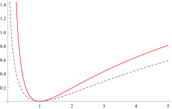
The loss function $d_{\Gamma}(x_{1},x_{2})$ is also called Itakura-Saito distance [13], and has proved to play an important role in linear inverse problems as investigated by Csiszár [14]. To visualize this loss function, we fix $x_{1}=1$ and vary $x_{2}$ to obtain the solid curve in Figure 1.

Refer to caption — Fig. 1: Visualization of $d_{\mathsf{NB}}(1,x)$ and $d_{\Gamma}(1,x)$ . The solid curve is $d_{\Gamma}(1,x)$ . The dashed curve is $d_{\mathsf{NB}}(1,x)$ .

For negative binomial channels, we have $\kappa_{\mathsf{NB}}(\theta)=\ln\left(\frac{\frac{1}{2}}{1-\frac{1}{2}e^{\theta}}\right)$ . The Fenchel–Legendre dual of $\kappa_{\mathsf{NB}}(\theta)$ is

\phi_{\mathsf{NB}}(x)=x\ln x-(1+x)\ln(1+x)+x\ln 2+\ln 2,\quad x\geq 0.

(118)

Hence,

\displaystyle d_{\mathsf{NB}}(x_{1},x_{2})=x_{1}\ln\left(\frac{x_{1}}{x_{2}}\right)+(1+x_{1})\ln\left(\frac{1+x_{2}}{1+x_{1}}\right).

(119)

To visualize $d_{\mathsf{NB}}(x_{1},x_{2})$ , we fix $x_{1}=1$ and vary $x_{2}$ to obtain the dashed curve in Figure 1.

VI-B Relations to other generalizations

We briefly discuss the key differences between our approach and existing approaches to establishing information-estimation results in channels beyond Gaussian and Poisson. From now on we discuss the general natural exponential families introduced in Section II-B and do not constrain ourselves to the discrete-time Lévy channels. Targeting at several members of the natural exponential family, [12] took a view different from ours. They called an input amplification factor $a$ to be the parameter of interest. In other words, suppose $ax_{1}=\kappa^{\prime}(\theta_{1}),ax_{2}=\kappa^{\prime}(\theta_{2}),a>0$ , and consider deterministic inputs $ax_{1},ax_{2}$ , we have

D(P_{1}\|P_{2})=\phi(ax_{1})-\phi(ax_{2})-\phi^{\prime}(ax_{2})(ax_{1}-ax_{2}),

(120)

and the parameter $a$ is the parameter with respect to which [12] analyze the derivatives of mutual information and relative entropy.

Essentially, [12] worked on generalizing (120) to random inputs $X$ . However, it seems to the authors that even in the deterministic inputs case (120), the parameter $a$ may not display consistent properties for different channel models. Indeed, if we take derivatives on both sides of (120), we will obtain

a\frac{\partial}{\partial a}D(P_{1}\|P_{2})=d_{f}(ax_{1},ax_{2}),

(121)

where $f(x)=x\phi^{\prime}(x),d_{f}(x,y)=f(x)-f(y)-f^{\prime}(y)(x-y)$ . However, $\phi(x)$ being a convex function does not imply $f(x)=x\phi^{\prime}(x)$ is also a convex function, hence $d_{f}(x,y)$ may not be a Bregman divergence, and is not necessarily non-negative. Coincidentally, for Gaussian and Poisson models, the Bregman divergence generated by $x\phi^{\prime}(x)$ and $\phi(x)$ are equal up to a multiplicative factor. Indeed, we have

	$\displaystyle\phi(x)=\frac{1}{2}x^{2},$	$\displaystyle\quad d_{\phi}(x,y)=\frac{1}{2}(x-y)^{2},$		(122)
	$\displaystyle x\phi^{\prime}(x)=x^{2},$	$\displaystyle\quad d_{x\phi^{\prime}(x)}(x,y)=(x-y)^{2},$		(123)

for the Gaussian model, and

	$\displaystyle\phi(x)=x\ln x-x+1,$	$\displaystyle\quad d_{\phi}(x,y)=x\ln\left(\frac{x}{y}\right)-x+y,$		(124)
	$\displaystyle x\phi^{\prime}(x)=x\ln x,$	$\displaystyle\quad d_{x\phi^{\prime}(x)}(x,y)=x\ln\left(\frac{x}{y}\right)-x+y,$		(125)

for the Poisson model.

The Bregman divergences listed in [12] for binomial and negative binomial models are all Bregman divergences generated by $x\phi^{\prime}(x)$ , and it so happens that they are both strictly convex. However, if we consider the gamma distribution, we have

\phi_{\Gamma}(x)=x-1-\ln(x),

(126)

which implies

f(x)=x\phi_{\Gamma}^{\prime}(x)=x-1,\quad d_{f}(x,y)\equiv 0.

(127)

As a consequence of this parametrization, results in [12] do not take the forms of (1) and (3).

Further, we can show that even if we consider random inputs in the gamma distribution, if we follow the definition of parameter $a$ in [12], we would obtain that the mutual information between input and output is invariant with respect to the parameter $a$ . In our definition of the gamma channel, we have

Y_{\gamma}|X\sim\Gamma(\gamma,X),

(128)

however, if we follow [12], then we have

Y_{a}|X\sim\Gamma(k,aX/k),

(129)

where $k$ is some fixed positive constant.

Lemma 21

Suppose $P,Q$ are two probability measures of non-negative random variable $X$ . If we have $Y_{a}|X\sim\Gamma(k,aX/k),k>0$ , then

	$\displaystyle\frac{\partial}{\partial a}I(X;Y_{a})$	$\displaystyle\equiv 0$		(130)
	$\displaystyle\frac{\partial}{\partial a}D(P_{Y_{a}}\\|Q_{Y_{a}})$	$\displaystyle\equiv 0.$		(131)

Lemma 21 shows the parameterization in [12] may lead to some strange results that do not capture the infinite-divisibility of the gamma distribution.

We hope to have convinced the reader that the parametrization in our framework is natural and captures the core properties of the Gaussian and Poisson distributions. In fact, we conjecture that discrete-time Lévy channels are the largest family of channels for which one can establish information-estimation results paralleling all existing results in the Gaussian and Poisson observation models.

VII Proofs

VII-A Proof of Theorem 10

Theorem 10 can be obtained via direct application of Theorem 12. Indeed, mutual information $I(X;Y_{\gamma})$ is expressible as

I(X;Y_{\gamma})=\mathbb{E}_{X}D(P_{Y_{\gamma}|X}\|P_{Y_{\gamma}}),

(132)

where $P_{Y_{\gamma}|X}$ is the marginal distribution of output of the Lévy channel under point mass input $\delta_{X}$ , and $P_{Y_{\gamma}}$ is the marginal distribution of $Y_{\gamma}$ under input $P_{X}$ .

It suffices to verify that the conditions of Theorem 12 are satisfied for $P$ corresponding to point mass $\delta_{X}$ and $Q$ corresponding to input distribution $P_{X}$ . Indeed, it suffices to show that with probability one,

	$\displaystyle\int_{0}^{\gamma}\mathbb{E}_{Y_{\alpha}\|X}\left(\phi^{\prime}(X)-\mathbb{E}[\phi^{\prime}(X)\|Y_{\alpha}]\right)^{2}d\alpha$	$\displaystyle<\infty$		(133)
	$\displaystyle\int_{0}^{\gamma}\int_{\mathbb{R}}\mathbb{E}_{Y_{\alpha}\|X}\left(e^{\phi^{\prime}(X)z}\hbox{$\left\|\vbox to0.0pt{}\right.$}\ln\left(\frac{e^{\phi^{\prime}(X)z}}{\mathbb{E}_{P}[e^{\phi^{\prime}(X)z}\|Y_{\alpha}]}\right)\hbox{$\left\|\vbox to0.0pt{}\right.$}\right)\nu(dz)d\alpha$	$\displaystyle<\infty.$		(134)

We have the following lemma.

Lemma 22

Suppose $\sigma\neq 0$ and $\mathbb{E}_{P}(\phi^{\prime}(X))^{2}<\infty$ . Then with probability one for any $0<\gamma<\infty$ ,

\displaystyle\int_{0}^{\gamma}\mathbb{E}_{Y_{\alpha}|X}\left(\phi^{\prime}(X)-\mathbb{E}[\phi^{\prime}(X)|Y_{\alpha}]\right)^{2}d\alpha

\displaystyle<\infty.

(135)

Suppose $\int_{\mathbb{R}}\nu(dz)<\infty$ and $\mathbb{E}_{P}\int_{\mathbb{R}}|\phi^{\prime}(X)z|e^{\phi^{\prime}(X)z}\nu(dz)<\infty$ . Then with probability one for any $0<\gamma<\infty$ ,

\displaystyle\int_{0}^{\gamma}\int_{\mathbb{R}}\mathbb{E}_{Y_{\alpha}|X}\left(e^{\phi^{\prime}(X)z}\hbox{$\left|\vbox to0.0pt{}\right.$}\ln\left(\frac{e^{\phi^{\prime}(X)z}}{\mathbb{E}_{P}[e^{\phi^{\prime}(X)z}|Y_{\alpha}]}\right)\hbox{$\left|\vbox to0.0pt{}\right.$}\right)\nu(dz)d\alpha

\displaystyle<\infty.

(136)

Suppose $\int_{\mathbb{R}}\nu(dz)=\infty$ , $\mathbb{E}_{P}\int_{\mathbb{R}}|\phi^{\prime}(X)z|e^{\phi^{\prime}(X)z}\nu(dz)<\infty$ , and

\displaystyle\int_{0}^{\gamma}\int_{\mathbb{R}}\mathbb{E}\left(e^{\phi^{\prime}(X)z}\hbox{$\left|\vbox to0.0pt{}\right.$}\ln\mathbb{E}_{P}[e^{\phi^{\prime}(X)z}|Y_{\alpha}]\hbox{$\left|\vbox to0.0pt{}\right.$}\right)\nu(dz)d\alpha

\displaystyle<\infty.

(137)

Then with probability one for any $0<\gamma<\infty$ ,

\displaystyle\int_{0}^{\gamma}\int_{\mathbb{R}}\mathbb{E}_{Y_{\alpha}|X}\left(e^{\phi^{\prime}(X)z}\hbox{$\left|\vbox to0.0pt{}\right.$}\ln\left(\frac{e^{\phi^{\prime}(X)z}}{\mathbb{E}_{P}[e^{\phi^{\prime}(X)z}|Y_{\alpha}]}\right)\hbox{$\left|\vbox to0.0pt{}\right.$}\right)\nu(dz)d\alpha

\displaystyle<\infty.

(138)

Proof:

1.

The desired claim follows from showing

$\displaystyle\int_{0}^{\gamma}\mathbb{E}(\phi^{\prime}(X)-\mathbb{E}[\phi^{\prime}(X)|Y_{\alpha}])^{2}d\alpha<\infty,$ (139)

which is implied by observing that $\mathbb{E}(\phi^{\prime}(X)-\mathbb{E}[\phi^{\prime}(X)|Y_{\alpha}])^{2}\leq\mathbb{E}(\phi^{\prime}(X))^{2}$ .

It suffices to prove that

\displaystyle\int_{0}^{\gamma}\int_{\mathbb{R}}\mathbb{E}\left(e^{\phi^{\prime}(X)z}\hbox{$\left|\vbox to0.0pt{}\right.$}\ln\mathbb{E}_{P}[e^{\phi^{\prime}(X)z}|Y_{\alpha}]\hbox{$\left|\vbox to0.0pt{}\right.$}\right)\nu(dz)d\alpha

\displaystyle<\infty.

(140)

We have

\displaystyle\int_{0}^{\gamma}\int_{\mathbb{R}}\mathbb{E}\left(e^{\phi^{\prime}(X)z}\hbox{$\left|\vbox to0.0pt{}\right.$}\ln\mathbb{E}_{P}[e^{\phi^{\prime}(X)z}|Y_{\alpha}]\hbox{$\left|\vbox to0.0pt{}\right.$}\right)\nu(dz)d\alpha

\displaystyle=\int_{0}^{\gamma}\int_{\mathbb{R}}\mathbb{E}\left(\mathbb{E}_{P}[e^{\phi^{\prime}(X)z}|Y_{\alpha}]\hbox{$\left|\vbox to0.0pt{}\right.$}\ln\mathbb{E}_{P}[e^{\phi^{\prime}(X)z}|Y_{\alpha}]\hbox{$\left|\vbox to0.0pt{}\right.$}\right)\nu(dz)d\alpha

(141)

The claim follows from observing that

(a)

For any $x\geq 0$ , $x|\ln x|\leq-2x\ln x\mathbbm{1}_{0\leq x\leq 1}+x\ln x$ ;
(b)

For $x\in[0,1]$ , $0\leq-2x\ln x\leq\frac{2}{e}$ ;
(c)

$\int_{\mathbb{R}}\nu(dz)<\infty$ ;
(d)

The function $x\ln x$ is convex on $\mathbb{R}_{+}$ ; hence $\mathbb{E}[X]\ln(\mathbb{E}[X])\leq\mathbb{E}[X\ln X]$ ;
(e)

$\mathbb{E}_{P}\int_{\mathbb{R}}|\phi^{\prime}(X)z|e^{\phi^{\prime}(X)z}\nu(dz)<\infty$ .

3.

It follows from the triangle inequality.

∎

Thus,

I(X;Y_{\gamma})=\int_{0}^{\gamma}\mathbb{E}_{P}\ell_{\mathcal{L}}(X,\hat{X}_{\alpha}^{P})d\alpha.

(143)

The final claim follows from taking derivatives on both sides with respect to $\gamma$ .

VII-B Proof of Theorem 11

According to Theorem 10, for any $\gamma$ ,

I(X;Y_{\gamma})=\int_{0}^{\gamma}\mathbb{E}_{P}\ell_{\mathcal{L}}(X,\hat{X}_{\alpha}^{P})d\alpha.

(144)

Taking $\gamma\to\infty$ on both sides, we have

\lim_{\gamma\to\infty}I(X;Y_{\gamma})=\int_{0}^{\infty}\mathbb{E}_{P}\ell_{\mathcal{L}}(X,\hat{X}_{\alpha}^{P})d\alpha,

(145)

For discrete random variables $X$ ,

\lim_{\gamma\to\infty}I(X;Y_{\gamma})=H(X).

(146)

VII-C Proof of Theorem 12

Applying the coupling in Lemma 8, we define the non-negative martingale process with respect to filtration $\mathcal{F}_{t}={\cal F}_{t}^{Y}\vee\sigma\{X\}$ :

L_{t}\doteq\frac{dP^{[0,t]}_{\theta}}{dP^{[0,t]}_{0}}(Y_{s},0\leq s\leq t)=e^{\theta Y_{t}-t\kappa(\theta)},

(147)

where $\{Y_{s}:0\leq s\leq t\}$ follows distribution $P^{[0,t]}_{0}$ . The random variable $\theta=\phi^{\prime}(X)$ is a function of the input $X$ (see Definition 5). Note that $A\vee B$ denotes the smallest $\sigma$ -algebra that contains both $\sigma$ -algebras $A$ and $B$ , and $\mathcal{F}_{t}^{Y}$ denotes the filtration $\sigma\{Y_{s}:0\leq s\leq t\}$ .

Applying (12) in Lemma 2, Lemma 3 and plugging those in the expression of $L_{t}$ , we have

	$\displaystyle L_{t}$	$\displaystyle=e^{\theta\left(at+\sigma W_{t}+\int_{0}^{t}\int_{\|z\|<1}z(\mu(ds,dz)-\nu(dz)ds)+\int_{0}^{t}\int_{\|z\|\geq 1}z\mu(ds,dz)\right)-t\kappa(\theta)}$		(148)
		$\displaystyle=e^{\sigma\theta W_{t}-\frac{1}{2}\sigma^{2}\theta^{2}t+\int_{0}^{t}\int_{\mathbb{R}}\left(\theta z\mu(ds,dz)-(e^{\theta z}-1)\nu(dz)ds\right)}.$		(149)

We have the following It $\hat{\mathrm{o}}$ ’s formula for general semimartingales, and we refer the readers to [15] for the general theory of semimartingales.

Lemma 23

[15, Thm. 6.46] If $\{Z(t):t\geq 0\}$ is a semimartingale and $f(x)\in C^{2}(\mathbb{R})$ , then

\displaystyle f(Z(t))-f(Z(0))

\displaystyle=\int_{0}^{t}f^{\prime}(Z_{-})dZ+\frac{1}{2}\int_{0}^{t}f^{\prime\prime}(Z_{-})d[Z]^{c}+\sum_{0<s\leq t}\left(f(Z(s))-f(Z(s-))-f^{\prime}(Z(s-))\Delta Z(s)\right),

(150)

where the process $[Z]^{c}_{t}$ is the quadratic variation process of the continuous part of the semimartingale $Z(t)$ , $\Delta Z(s)=Z(s)-Z(s-)$ , and $Z(s-)=\lim_{u\to s-}Z(u)$ .

Setting

$\displaystyle Z(t)$	$\displaystyle=\sigma\theta W_{t}-\frac{1}{2}\sigma^{2}\theta^{2}t+D(t)$	(151)
$\displaystyle D(t)$	$\displaystyle=\int_{0}^{t}\int_{\mathbb{R}}\left(\theta z\mu(ds,dz)-(e^{\theta z}-1)\nu(dz)ds\right)$	(152)
$\displaystyle f(z)$	$\displaystyle=e^{z},$	(153)

we know

\displaystyle[Z]_{t}^{c}

\displaystyle=\sigma^{2}\theta^{2}t.

(154)

Applying Lemma 23, we get the following representation of the martingale $L_{t}$ :

$\displaystyle L_{t}$	$\displaystyle=1+\int_{0}^{t}L_{s-}dZ(t)+\frac{1}{2}\sigma^{2}\theta^{2}\int_{0}^{t}L_{s-}ds+\sum_{0<s\leq t}f(Z(s-))\left(\frac{f(Z(s))}{f(Z(s-))}-1-\Delta Z(s)\right)$	(155)
	$\displaystyle=1+\int_{0}^{t}\sigma\theta L_{s-}dW_{s}+\int_{0}^{t}L_{s-}dD(s)+\sum_{0<s\leq t}L_{s-}\left(e^{\Delta Z(s)}-1-\Delta Z(s)\right)$	(156)
	$\displaystyle=1+\int_{0}^{t}\sigma\theta L_{s-}dW_{s}+\int_{0}^{t}L_{s-}dD(s)+\sum_{0<s\leq t}L_{s-}\left(e^{\theta z}-1-\theta z\right)\mu(ds,dz)$	(157)
	$\displaystyle=1+\int_{0}^{t}L_{s-}dM_{t},$	(158)

where

	$\displaystyle M_{t}$	$\displaystyle=\sigma\theta W_{t}+\int_{0}^{t}\int_{\mathbb{R}}\left(\theta z\mu(ds,dz)-(e^{\theta z}-1)\nu(dz)ds+e^{\theta z}\mu(ds,dz)-(1+\theta z)\mu(ds,dz)\right)$		(159)
		$\displaystyle=\sigma\theta W_{t}+\int_{0}^{t}\int_{\mathbb{R}}(e^{\theta z}-1)\left(\mu(ds,dz)-\nu(dz)ds\right).$		(160)

The equation (158) is called the Doléans–Dade equation [15, Def. 6.53], whose solution is unique and is given by

L_{t}=e^{\varphi_{t}},

(161)

where

\varphi_{t}=M_{t}-\frac{1}{2}[M]_{t}^{c}+\sum_{s\leq t}\left(\ln(1+\Delta M_{s})-\Delta M_{s}\right).

(162)

Plugging $M_{t}$ into the general solution, one can also verify that $L_{t}$ is indeed the unique solution.

In order to characterize the relative entropy, we need to compute the marginal distribution of $Y_{t}$ . Let $P_{Y_{t}}$ denote the probability measure of $\{Y_{s}:0\leq s\leq t\}$ with respect to the filtration $\mathcal{F}_{t}^{Y}$ when the input $X$ has distribution $P$ , $Q_{Y_{t}}$ denote that when the input has distribution $Q$ , and $R_{Y_{t}}$ denote that when there the input corresponds to $\theta=0$ .

We have the following lemma.

Lemma 24

Given probability space $(\Omega,\mathcal{F},\mathbb{P})$ , consider another probability measure $Q$ such that $Q\ll P$ . Denote the Radon–Nikodym derivative as $Z=\frac{d\mathbb{Q}}{d\mathbb{P}}$ . Then,

1.

For sub- $\sigma$ -algebra $\mathcal{G}\subset\mathcal{F}$ , we have

$\displaystyle\frac{d\mathbb{Q}_{|\mathcal{G}}}{d\mathbb{P}_{|\mathcal{G}}}$ $\displaystyle=\mathbb{E}_{P}[Z|\mathcal{G}].$ (163)
2.

For any $\mathcal{F}$ -measurable random variable $X$ , we have

$\displaystyle\mathbb{E}_{P}[ZX|\mathcal{G}]$ $\displaystyle=\mathbb{E}_{P}[Z|\mathcal{G}]\mathbb{E}_{Q}[X|\mathcal{G}].$ (164)

It follows from Lemma 24 that

\frac{dP_{Y_{t}}}{dR_{Y_{t}}}=\mathbb{E}_{R}\left[L_{t}|{\cal F}_{t}^{Y}\right],\quad R_{Y_{t}}-a.s.

(165)

Denote $\frac{dP_{Y_{t}}}{dR_{Y_{t}}}$ by $\bar{L}_{t}^{P}$ . We have

L_{t}=1+\int_{0}^{t}\sigma L_{s-}\theta dW_{s}+\int_{0}^{t}L_{s-}\left(\int_{\mathbb{R}}(e^{\theta z}-1)(\mu(ds,dz)-\nu(dz)ds)\right).

(166)

Taking conditional expectations with respect to ${\cal F}_{t}^{Y}$ on both sides under $R_{Y_{t}}$ , noting that $W_{t}$ and $\mu(dt,sz)$ are measurable with respect to $\mathcal{F}_{t}^{Y}$ and applying the Fubini-type theorem for conditional expectations in [16, Thm. 2], we have

\bar{L}_{t}^{P}=1+\int_{0}^{t}\sigma\mathbb{E}_{R}[L_{s-}\theta|{\cal F}_{s}^{Y}]dW_{s}+\int_{0}^{t}\left(\int_{\mathbb{R}}(\mathbb{E}_{R}[L_{s-}(e^{\theta z}-1)|{\cal F}_{s}^{Y}])(\mu(ds,dz)-\nu(dz)ds)\right).

(167)

It follows from Lemma 24 that

	$\displaystyle\mathbb{E}_{R}[L_{s-}\theta\|{\cal F}_{s}^{Y}]$	$\displaystyle=\bar{L}^{P}_{s-}\mathbb{E}_{P}[\theta\|{\cal F}_{s}^{Y}]$		(168)
	$\displaystyle\mathbb{E}_{R}[L_{s-}(e^{\theta z}-1)\|{\cal F}_{s}^{Y}])$	$\displaystyle=\bar{L}^{P}_{s-}(\mathbb{E}_{P}[e^{\theta z}\|{\cal F}_{s}^{Y}]-1),$		(169)

which implies

\bar{L}_{t}^{P}=1+\int_{0}^{t}\sigma\bar{L}^{P}_{s-}\mathbb{E}_{P}[\theta|{\cal F}_{s}^{Y}]dW_{s}+\int_{0}^{t}\bar{L}^{P}_{s-}\left(\int_{\mathbb{R}}(\mathbb{E}_{P}[e^{\theta z}|{\cal F}_{s}^{Y}]-1)(\mu(ds,dz)-\nu(dz)ds)\right).

(170)

Solving this stochastic differential equation using the general solutions given by (161) and (162), we have

\bar{L}_{t}^{P}=e^{\rho_{t}^{P}},

(171)

where

\rho_{t}^{P}=\sigma\int_{0}^{t}\mathbb{E}_{P}[\theta|{\cal F}_{s}^{Y}]dW_{s}-\frac{1}{2}\sigma^{2}\int_{0}^{t}(\mathbb{E}_{P}[\theta|{\cal F}_{s}^{Y}])^{2}ds+\int_{0}^{t}\int_{\mathbb{R}}\left(\ln\left(\mathbb{E}_{P}[e^{\theta z}|{\cal F}_{s}^{Y}]\right)\mu(ds,dz)-(\mathbb{E}_{P}[e^{\theta z}|{\cal F}_{s}^{Y}]-1)\nu(dz)ds\right).

(172)

We have similar expressions for $\bar{L}_{t}^{Q}=\frac{dQ_{Y_{t}}}{dR_{Y_{t}}}$ . In order to calculate the relative entropy, we have

$\displaystyle\ln\frac{dP_{Y_{t}}}{dQ_{Y_{t}}}$	$\displaystyle=\ln\left(\frac{dP_{Y_{t}}}{dR_{Y_{t}}}\frac{dR_{Y_{t}}}{dQ_{Y_{t}}}\right)$	(173)
	$\displaystyle=\ln\frac{dP_{Y_{t}}}{dR_{Y_{t}}}-\ln\frac{dQ_{Y_{t}}}{dR_{Y_{t}}}$	(174)
	$\displaystyle=\rho_{t}^{P}-\rho_{t}^{Q}$	(175)
	$\displaystyle=\sigma\int_{0}^{t}\left(\mathbb{E}_{P}[\theta\|{\cal F}_{s}^{Y}]-\mathbb{E}_{Q}[\theta\|{\cal F}_{s}^{Y}]\right)dW_{s}-\frac{1}{2}\sigma^{2}\int_{0}^{t}\left(\mathbb{E}_{P}[\theta\|{\cal F}_{s}^{Y}]^{2}-\mathbb{E}_{Q}[\theta\|{\cal F}_{s}^{Y}]^{2}\right)ds$	(176)
	$\displaystyle\quad+\int_{0}^{t}\int_{\mathbb{R}}\left(\ln\left(\frac{\mathbb{E}_{P}[e^{\theta z}\|{\cal F}_{s}^{Y}]}{\mathbb{E}_{Q}[e^{\theta z}\|{\cal F}_{s}^{Y}]}\right)\mu(ds,dz)-(\mathbb{E}_{P}[e^{\theta z}\|{\cal F}_{s}^{Y}]-\mathbb{E}_{Q}[e^{\theta z}\|{\cal F}_{s}^{Y}])\nu(dz)ds\right)$	(177)

It follows from [17, Chap. 4, Sec. 6, Thm. 5] that under probability measure $P_{Y_{t}}$ , the process

\tilde{W}_{t}=W_{t}-\int_{0}^{t}\mathbb{E}_{P}[\theta|{\cal F}_{s}^{Y}]ds

(178)

is a Brownian motion. Also, under $P_{Y_{t}}$ , the compensator of $\mu(ds,dz)$ is no longer $\nu(dz)ds$ , but $\mathbb{E}_{P}[e^{\theta z}|{\cal F}_{s}^{Y}]\nu(dz)ds$ .

Bearing these in mind, we represent $\ln\frac{dP_{Y_{t}}}{dQ_{Y_{t}}}$ as

$\displaystyle\ln\frac{dP_{Y_{t}}}{dQ_{Y_{t}}}$	$\displaystyle=\sigma\int_{0}^{t}\left(\mathbb{E}_{P}[\theta\|{\cal F}_{s}^{Y}]-\mathbb{E}_{Q}[\theta\|{\cal F}_{s}^{Y}]\right)d\tilde{W}_{s}+\frac{1}{2}\sigma^{2}\int_{0}^{t}\left(\mathbb{E}_{P}[\theta\|{\cal F}_{s}^{Y}]-\mathbb{E}_{Q}[\theta\|{\cal F}_{s}^{Y}]\right)^{2}ds$	(179)
	$\displaystyle\quad+\int_{0}^{t}\int_{\mathbb{R}}\ln\left(\frac{\mathbb{E}_{P}[e^{\theta z}\|{\cal F}_{s}^{Y}]}{\mathbb{E}_{Q}[e^{\theta z}\|{\cal F}_{s}^{Y}]}\right)\left(\mu(ds,dz)-\mathbb{E}_{P}[e^{\theta z}\|{\cal F}_{s}^{Y}]\nu(dz)ds\right)$	(180)
	$\displaystyle\quad+\int_{0}^{t}\int_{\mathbb{R}}\left(\mathbb{E}_{P}[e^{\theta z}\|{\cal F}_{s}^{Y}]\ln\left(\frac{\mathbb{E}_{P}[e^{\theta z}\|{\cal F}_{s}^{Y}]}{\mathbb{E}_{Q}[e^{\theta z}\|{\cal F}_{s}^{Y}]}\right)-\mathbb{E}_{P}[e^{\theta z}\|{\cal F}_{s}^{Y}]+\mathbb{E}_{Q}[e^{\theta z}\|{\cal F}_{s}^{Y}]\right)\nu(dz)ds$	(181)

Now we take expectations with respect to $P_{Y_{t}}$ on both sides. If the integrand of the stochastic integral with respect to $\tilde{W}_{s}$ is square integrable, i.e.

\mathbb{E}_{P}\int_{0}^{t}\left(\mathbb{E}_{P}[\theta|{\cal F}_{s}^{Y}]-\mathbb{E}_{Q}[\theta|{\cal F}_{s}^{Y}]\right)^{2}ds<\infty,

(182)

then

\sigma\int_{0}^{t}\left(\mathbb{E}_{P}[\theta|{\cal F}_{s}^{Y}]-\mathbb{E}_{Q}[\theta|{\cal F}_{s}^{Y}]\right)d\tilde{W}_{s}

(183)

is a martingale, hence has mean zero.

Meanwhile, according to [18, Thm 18.7], if

\int_{0}^{t}\int_{\mathbb{R}}\mathbb{E}_{P}\left(\mathbb{E}_{P}[e^{\theta z}|{\cal F}_{s}^{Y}]\hbox{$\left|\vbox to0.0pt{}\right.$}\ln\left(\frac{\mathbb{E}_{P}[e^{\theta z}|{\cal F}_{s}^{Y}]}{\mathbb{E}_{Q}[e^{\theta z}|{\cal F}_{s}^{Y}]}\right)\hbox{$\left|\vbox to0.0pt{}\right.$}\right)\nu(dz)ds<\infty,

(184)

then

\int_{0}^{t}\int_{\mathbb{R}}\ln\left(\frac{\mathbb{E}_{P}[e^{\theta z}|{\cal F}_{s}^{Y}]}{\mathbb{E}_{Q}[e^{\theta z}|{\cal F}_{s}^{Y}]}\right)\left(\mu(ds,dz)-\mathbb{E}_{P}[e^{\theta z}|{\cal F}_{s}^{Y}]\nu(dz)ds\right)

(185)

is a zero mean martingale.

Both conditions are guaranteed by the assumptions. Hence,

$\displaystyle D(P_{Y_{t}}\\|Q_{Y_{t}})$	$\displaystyle=\frac{1}{2}\sigma^{2}\int_{0}^{t}\mathbb{E}_{P}\left(\mathbb{E}_{P}[\theta\|{\cal F}_{s}^{Y}]-\mathbb{E}_{Q}[\theta\|{\cal F}_{s}^{Y}]\right)^{2}ds$	(186)
	$\displaystyle\quad+\int_{0}^{t}\int_{\mathbb{R}}\mathbb{E}_{P}\left(\mathbb{E}_{P}[e^{\theta z}\|{\cal F}_{s}^{Y}]\ln\left(\frac{\mathbb{E}_{P}[e^{\theta z}\|{\cal F}_{s}^{Y}]}{\mathbb{E}_{Q}[e^{\theta z}\|{\cal F}_{s}^{Y}]}\right)-\mathbb{E}_{P}[e^{\theta z}\|{\cal F}_{s}^{Y}]+\mathbb{E}_{Q}[e^{\theta z}\|{\cal F}_{s}^{Y}]\right)\nu(dz)ds.$	(187)
	$\displaystyle=\mathbb{E}_{P}\int_{0}^{t}\ell_{\mathcal{L}}(X,\hat{X}_{s}^{Q})-\ell_{\mathcal{L}}(X,\hat{X}_{s}^{P})ds,$	(188)

where in the last step we have used the following facts:

\displaystyle\mathbb{E}_{P}(X-\mathbb{E}_{Q}[X|Y])^{2}-\mathbb{E}_{P}(X-\mathbb{E}_{P}[X|Y])^{2}

\displaystyle=\mathbb{E}_{P}\left(\mathbb{E}_{P}[X|Y]-\mathbb{E}_{Q}[X|Y]\right)^{2},

(189)

\displaystyle\mathbb{E}_{P}\ell_{{\cal P}}(X,\mathbb{E}_{Q}[X|Y])-\mathbb{E}_{P}\ell_{{\cal P}}(X,\mathbb{E}_{P}[X|Y])

\displaystyle=\mathbb{E}_{P}\ell_{{\cal P}}(\mathbb{E}_{P}[X|Y],\mathbb{E}_{Q}[X|Y]).

(190)

VII-D Proof of Theorem 13

According to Theorem 12, we know for all $\gamma<\infty$ ,

D(P_{Y_{\gamma}}||Q_{Y_{\gamma}})=\int_{0}^{\gamma}\mathbb{E}_{P}[\ell_{{\cal L}}(X,\hat{X}^{Q}_{\alpha})-\ell_{{\cal L}}(X,\hat{X}^{P}_{\alpha})]\,d\alpha.

(191)

We will first show that

\lim_{\gamma\to\infty}D(P_{Y_{\gamma}}||Q_{Y_{\gamma}})=D(P\|Q).

(192)

Note that

$\displaystyle D(P_{Y_{\gamma}}\|\|Q_{Y_{\gamma}})$	$\displaystyle\leq D(P_{X,Y_{\gamma}}\\|Q_{X,Y_{\gamma}})$	(193)
	$\displaystyle=D(P\\|Q)+D(P_{Y_{\gamma}\|X}\\|Q_{Y_{\gamma}\|X}\|P)$	(194)
	$\displaystyle=D(P\\|Q),$	(195)

where the last equality is due to the fact that $P_{X}$ -a.s. $P_{Y_{\gamma}|X}=Q_{Y_{\gamma}|X}$ provided that $P\ll Q$ . The monotonicity of $D(P_{Y_{\gamma}}||Q_{Y_{\gamma}})$ (which follows from (191)) implies that the limit exists when $\gamma\to\infty$ , and

\lim_{\gamma\to\infty}D(P_{Y_{\gamma}}||Q_{Y_{\gamma}})\leq D(P\|Q).

(196)

On the other hand, by the Law of Large Numbers, $Y_{\gamma}/\gamma$ converges weakly to $X$ when $\gamma\to\infty$ . Since relative entropy is lower semi-continuous under weak convergence, we have

	$\displaystyle\liminf_{\gamma\to\infty}D(P_{Y_{\gamma}}\|\|Q_{Y_{\gamma}})$	$\displaystyle=\liminf_{\gamma\to\infty}D(P_{Y_{\gamma}/\gamma}\\|Q_{Y_{\gamma}/\gamma})$		(197)
		$\displaystyle\geq D(P\\|Q).$		(198)

We conclude that $\lim_{\gamma\to\infty}D(P_{Y_{\gamma}}||Q_{Y_{\gamma}})=D(P\|Q)$ .

Since

\lim_{\gamma\to\infty}\int_{0}^{\gamma}\mathbb{E}_{P}[\ell_{{\cal L}}(X,\hat{X}^{Q}_{\alpha})-\ell_{{\cal L}}(X,\hat{X}^{P}_{\alpha})]\,d\alpha=\int_{0}^{\infty}\mathbb{E}_{P}[\ell_{{\cal L}}(X,\hat{X}^{Q}_{\alpha})-\ell_{{\cal L}}(X,\hat{X}^{P}_{\alpha})]\,d\alpha,

(199)

we have

D(P\|Q)=\int_{0}^{\infty}\mathbb{E}_{P}[\ell_{{\cal L}}(X,\hat{X}^{Q}_{\alpha})-\ell_{{\cal L}}(X,\hat{X}^{P}_{\alpha})]\,d\alpha.

(200)

VII-E Proof of Lemma 21

We first prove that, in the gamma distribution indexed by $\Gamma(k,aX/k)$ , the following relationship holds:

a\frac{\partial p(y)}{\partial a}=-\frac{d(yp(y))}{dy}.

(201)

Indeed, we have

p(y)=\int_{\mathcal{X}}\frac{k^{k}y^{k-1}e^{-\frac{ky}{ax}}}{(ax)^{k}\Gamma(k)}dP_{X},

(202)

and

	$\displaystyle a\frac{\partial p(y)}{\partial a}$	$\displaystyle=\int_{\mathcal{X}}\frac{ak^{k}y^{k-1}}{\Gamma(k)}\left(\frac{e^{-\frac{ky}{ax}}\frac{ky}{xa^{2}}(ax)^{k}-k(ax)^{k-1}xe^{-\frac{ky}{ax}}}{(ax)^{2k}}\right)dP_{X}$		(203)
		$\displaystyle=\int_{\mathcal{X}}\frac{k^{k}y^{k-1}e^{-\frac{ky}{ax}}}{\Gamma(k)(ax)^{k}}\left(\frac{ky}{ax}-k\right)dP_{X},$		(204)

as well as

$\displaystyle-\frac{d(yp(y))}{dy}$	$\displaystyle=-\frac{d}{dy}\int_{\mathcal{X}}\frac{k^{k}y^{k}e^{-\frac{ky}{ax}}}{(ax)^{k}\Gamma(k)}dP_{X}$	(205)
	$\displaystyle=-\int_{\mathcal{X}}\frac{k^{k}e^{-\frac{ky}{ax}}}{(ax)^{k}\Gamma(k)}\left(ky^{k-1}-\frac{ky^{k}}{ax}\right)dP_{X}$	(206)
	$\displaystyle=\int_{\mathcal{X}}\frac{k^{k}y^{k-1}e^{-\frac{ky}{ax}}}{\Gamma(k)(ax)^{k}}\left(\frac{ky}{ax}-k\right)dP_{X}$	(207)
	$\displaystyle=a\frac{\partial p(y)}{\partial a}.$	(208)

Based on (201), we have the following steps:

$\displaystyle a\frac{\partial D(P_{Y}\\|Q_{Y})}{\partial a}$	$\displaystyle=-\int\frac{d(yp(y))}{dy}\ln\frac{p(y)}{q(y)}dy+\int\frac{p(y)}{q(y)}d(yq(y))$	(209)
	$\displaystyle=\int\ln q(y)d(yp(y))-\int\ln p(y)d(yp(y))+\int\frac{p(y)}{q(y)}d(yq(y))$	(210)
	$\displaystyle=-\int\frac{dq(y)}{q(y)}yp(y)+\int\frac{dp(y)}{p(y)}yp(y)+\int\frac{p(y)}{q(y)}(ydq(y)+q(y)dy)$	(211)
	$\displaystyle=-\int y\frac{p(y)}{q(y)}dq(y)+\int ydp(y)+\int y\frac{p(y)}{q(y)}dq(y)+\int p(y)dy$	(212)
	$\displaystyle=\int ydp(y)+1$	(213)
	$\displaystyle=\int\left[-\frac{\partial p(y)}{\partial a}\right]dy-\int p(y)dy+1$	(214)
	$\displaystyle=\frac{\partial}{\partial a}\int p(y)dy$	(215)
	$\displaystyle=0.$	(216)

The result for mutual information follows from expressing $I(X;Y_{a})$ via

I(X;Y_{a})=D(P_{Y_{a}|X}\|P_{Y_{a}}|P_{X}).

(217)

VII-F Proof of Lemma 24

The first claim follows from showing that for any $B\in\mathcal{G}$ ,

\displaystyle\mathbb{Q}(B)=\mathbb{E}_{P}[Z\mathbbm{1}_{B}]=\mathbb{E}_{P}[\mathbb{E}_{P}[Z\mathbbm{1}_{B}|\mathcal{G}]]=\mathbb{E}_{P}[\mathbb{E}_{P}[Z|\mathcal{G}]\mathbbm{1}_{B}]=\int_{B}\mathbb{E}_{P}[Z|\mathcal{G}]d\mathbb{P}.

(218)

Regarding the second claim, denote $Y=\mathbb{E}_{P}[Z|\mathcal{G}]$ . Then, for any $B\in\mathcal{G}$ , we have

$\displaystyle\int_{B}\mathbb{E}_{P}[ZX\|\mathcal{G}]d\mathbb{Q}$	$\displaystyle=\int_{B}Y\mathbb{E}_{P}[ZX\|\mathcal{G}]d\mathbb{P}$	(219)
	$\displaystyle=\mathbb{E}_{P}[\mathbb{E}_{P}[Y\mathbbm{1}_{B}ZX\|\mathcal{G}]]$	(220)
	$\displaystyle=\mathbb{E}_{P}[Y\mathbbm{1}_{B}ZX]$	(221)
	$\displaystyle=\mathbb{E}_{Q}[Y\mathbbm{1}_{B}X]$	(222)
	$\displaystyle=\mathbb{E}_{Q}[\mathbb{E}_{Q}[Y\mathbbm{1}_{B}X\|\mathcal{G}]]$	(223)
	$\displaystyle=\mathbb{E}_{Q}[Y\mathbbm{1}_{B}\mathbb{E}_{Q}[X\|\mathcal{G}]]$	(224)
	$\displaystyle=\int_{B}Y\mathbb{E}_{Q}[X\|\mathcal{G}]d\mathbb{Q}.$	(225)

Since $B\in\mathcal{G}$ is arbitrary, we have

\displaystyle\mathbb{E}_{P}[ZX|\mathcal{G}]

\displaystyle=Y\mathbb{E}_{Q}[X|\mathcal{G}].

(226)

VIII Conclusions

We have introduced the family of discrete-time Lévy channels, where the output conditioned on the input is a random variable having an infinitely divisible law. We establish new and general relations between fundamental information measures and optimal estimation loss for this class of channels, under natural and explicitly identified loss functions. We conjecture that the discrete-time Lévy channels are the largest family of channels admitting information-estimation relations that fully parallel the known results for the Gaussian and Poisson models. It would be an interesting challenge to prove our main results without using the tools from continuous time stochastic process theory.

Acknowledgment

We are grateful to the associate editor and the anonymous reviewers for various constructive suggestions that helped significantly improve the presentation of the paper.

References

[1] D. Guo, S. Shamai, and S. Verdú, “The interplay between information and estimation measures,” Foundations and Trends in Signal Processing, vol. 6, no. 4, pp. 243–429, 2013.
[2] A. J. Stam, “Some inequalities satisfied by the quantities of information of Fisher and Shannon,” Information and Control, vol. 2, pp. 101–112, 1959.
[3] D. Guo, S. Shamai, and S. Verdú, “Mutual information and minimum mean-square error in Gaussian channels,” Information Theory, IEEE Transactions on, vol. 51, no. 4, pp. 1261–1282, 2005.
[4] Y. Wu and S. Verdú, “Functional properties of minimum mean-square error and mutual information,” IEEE Transactions on Information Theory, vol. 58, no. 3, pp. 1289–1301, 2012.
[5] D. Guo, S. Shamai, and S. Verdú, “Mutual information and conditional mean estimation in Poisson channels,” Information Theory, IEEE Transactions on, vol. 54, no. 5, pp. 1837–1849, 2008.
[6] R. Atar and T. Weissman, “Mutual information, relative entropy, and estimation in the Poisson channel,” Information Theory, IEEE Transactions on, vol. 58, no. 3, pp. 1302–1318, 2012.
[7] S. Verdú, “Mismatched estimation and relative entropy,” Information Theory, IEEE Transactions on, vol. 56, no. 8, pp. 3712–3720, 2010.
[8] P. MacCullagh and J. A. Nelder, Generalized linear models. CRC press, 1989, vol. 37.
[9] K.-i. Sato, Lévy processes and infinitely divisible distributions. Cambridge university press, 1999.
[10] U. Küchler and M. Sorensen, Exponential families of stochastic processes. Springer, 1997, vol. 3.
[11] F. Nielsen and R. Nock, “Entropies and cross-entropies of exponential families,” in Image Processing (ICIP), 2010 17th IEEE International Conference on. IEEE, 2010, pp. 3621–3624.
[12] C. G. Taborda, D. Guo, and F. Perez-Cruz, “Information-estimation relationships over binomial and negative binomial models,” IEEE Transactions on Information Theory, vol. 60, no. 5, pp. 2630–2646, 2014.
[13] A. Banerjee, S. Merugu, I. S. Dhillon, and J. Ghosh, “Clustering with Bregman divergences,” The Journal of Machine Learning Research, vol. 6, pp. 1705–1749, 2005.
[14] I. Csiszár, “Why least squares and maximum entropy? an axiomatic approach to inference for linear inverse problems,” The Annals of Statistics, vol. 19, no. 4, pp. 2032–2066, 12 1991. [Online]. Available: http://dx.doi.org/10.1214/aos/1176348385
[15] P. Medvegyev, Stochastic integration theory. Oxford University Press on Demand, 2007, no. 14.
[16] T. Kailath, A. Segall, and M. Zakai, “Fubini-type theorems for stochastic integrals,” Sankhyā: The Indian Journal of Statistics, Series A, pp. 138–143, 1978.
[17] R. Liptser and A. Shiryaev, Theory of martingales. Kluwer Academic Publishers (Dordrecht and Boston), 1989, vol. 49.
[18] R. Liptser and A. N. Shiryaev, Statistics of Random Processes II: Applications, 2nd ed. Springer-Verlag, 2001.

	$\displaystyle\mathbb{E}[\ell_{{\cal L}}(X,\hat{x})\|\mathcal{H}]$	$\displaystyle=\sigma^{2}\ell_{{\cal G}}(\phi^{\prime}(X),\mathbb{E}[\phi^{\prime}(X)\|\mathcal{H}])+\int_{\mathbb{R}}\ell_{{\cal P}}(e^{\phi^{\prime}(X)z},\mathbb{E}[e^{\phi^{\prime}(X)z}\|\mathcal{H}])\nu(dz)$		(56)
		$\displaystyle\quad+\sigma^{2}\ell_{{\cal G}}(\mathbb{E}[\phi^{\prime}(X)\|\mathcal{H}],\hat{x}_{0})+\int_{\mathbb{R}}\ell_{{\cal P}}(\mathbb{E}[e^{\phi^{\prime}(X)z}\|\mathcal{H}],\hat{x}_{z})\nu(dz)$		(57)

	$\displaystyle\mathbb{E}_{R}[L_{s-}\theta\|{\cal F}_{s}^{Y}]$	$\displaystyle=\bar{L}^{P}_{s-}\mathbb{E}_{P}[\theta\|{\cal F}_{s}^{Y}]$		(168)
	$\displaystyle\mathbb{E}_{R}[L_{s-}(e^{\theta z}-1)\|{\cal F}_{s}^{Y}])$	$\displaystyle=\bar{L}^{P}_{s-}(\mathbb{E}_{P}[e^{\theta z}\|{\cal F}_{s}^{Y}]-1),$		(169)

$\displaystyle D(P_{Y_{\gamma}}\|\|Q_{Y_{\gamma}})$	$\displaystyle\leq D(P_{X,Y_{\gamma}}\\|Q_{X,Y_{\gamma}})$	(193)
	$\displaystyle=D(P\\|Q)+D(P_{Y_{\gamma}\|X}\\|Q_{Y_{\gamma}\|X}\|P)$	(194)
	$\displaystyle=D(P\\|Q),$	(195)

	$\displaystyle\liminf_{\gamma\to\infty}D(P_{Y_{\gamma}}\|\|Q_{Y_{\gamma}})$	$\displaystyle=\liminf_{\gamma\to\infty}D(P_{Y_{\gamma}/\gamma}\\|Q_{Y_{\gamma}/\gamma})$		(197)
		$\displaystyle\geq D(P\\|Q).$		(198)