Quality Sensitive Price Competition in Secondary Market Spectrum Oligopoly- Multiple Locations
Abstract
We investigate a spectrum oligopoly market where each primary seeks to sell secondary access to its channel at multiple locations. Transmission qualities of a channel evolve randomly. Each primary needs to select a price and a set of non-interfering locations (which is an independent set in the conflict graph of the region) at which to offer its channel without knowing the transmission qualities of the channels of its competitors. At each location each secondary selects a channel depending on the price and the quality of the channels. We formulate the above problem as a non-cooperative game. We consider two scenarios-i) when the region is small, ii) when the region is large. In the first setting, we focus on a class of conflict graphs, known as mean valid graphs which commonly arise when the region is small. We explicitly compute a symmetric Nash equilibrium (NE) that selects only a small number of independent sets with positive probability. The NE is threshold type in that primaries only choose independent set whose cardinality is greater than a certain threshold. The threshold on the cardinality increases with increase in quality of the channel on sale. We show that the symmetric NE strategy profile is unique in a special class of conflict graphs (linear graph) which commonly arises in practice. In the second setting, we consider node symmetric conflict graphs which arises when the number of locations is large (potentially, infinite). We explicitly compute a symmetric NE that randomizes equally among the maximum independent sets at a given channel state vector. In the NE a primary only selects the maximum independent set at a given channel state vector. We show that the two symmetric NEs computed in two settings exhibit important structural difference. We numerically evaluate the ratio of the expected payoff attained by primaries in the game and the payoff attained by primaries when all the primaries collude.
Index Terms:
Game Theory, Nash Equilibrium, Secondary Spectrum Access, Quality of Service, Conflict Graph, Random Graphs, Independent Sets, Automorphism, Isomorphism, Branching Process.I Introduction
I-A Motivation
Secondary access of the spectrum where license holders (primaries) allow unlicensed users (secondaries) to use their channels can enhance the efficiency of the spectrum usage. However, secondary access will only proliferate when it is rendered profitable to the primaries. We investigate a spectrum oligopoly where primaries lease their spectrum to secondaries in lieu of financial remuneration. Each primary owns a channel throughout a large region consisting of several locations. The channel of a primary provides a transmission rate to a secondary depending on the state which evolves randomly and reflects the usage of the primary as well as the transmission rate due to fading. We consider the state of a channel is or where higher state corresponds to higher transmission rate. A secondary receives a payoff from a channel depending on the transmission rate offered by the channel and the price quoted by the primary. Secondaries buy those channels which give them the highest payoff, which leads to a competition among primaries.
Price competition in economics and wireless setting ignore two important properties which distinguish spectrum oligopoly from standard oligopolies: First, a primary selects a price knowing only the state of its own channel; it is unaware of states of its competitors’ channels. Thus, if a primary quotes a high price, it will earn a large profit if it sells its channel, but it may not be able to sell at all; on the other hand a low price will enhance the probability of a sale but may also fetch lower profits in the event of a sale. Second, the same spectrum band can be utilized simultaneously at geographically dispersed locations without interference; but the same band can not be utilized simultaneously at interfering locations. This special feature known as spatial reuse adds another dimension in the strategic interaction as now a primary has to cull a set of non-interfering locations, which is denoted as an independent set in the conflict graph representation of the region[2]; at which to offer its channel apart from selecting a price at every node of that set. Intuitively, a primary would like to make its channel available at an independent set of the maximum size (cardinality). However, if the competition at the largest independent set is intense, a primary may achieve higher payoff by setting high price at small independent sets (where the competition is not so intense).
I-B Our Contributions
We devise the problem as a game in which each primary’s strategy space consists of independent set selection strategy and the pricing strategy at each node of the independent set when the channel is available for sale. When the channel is in state , the transmission rate is very low and thus, we consider the channel is not available for sale. We first show that there may exist multiple asymmetric NEs. Asymmetric NEs are difficult to implement in the symmetric game that we consider (Section II-E). We, therefore, focus only on finding symmetric NEs subsequently. We prove a separation theorem (Section III-C) which entails that the NE pricing strategy at each location can be uniquely computed if the independent set selection strategy is known. By virtue of our previous work [3, 4] which characterizes pricing strategies of primaries for different transmission rates when the region has only one location (i.e. no spatial reuse). We then focus only on the independent set selection strategy.
Scenario 1: We consider two possible scenarios (Section II-F). First, we consider the setting when the region is small consisting of few locations (Section IV). Therefore, the usage statistics and the propagation condition of a channel do not vary substantially over the region. Thus, we assume that the channel state is identical at each location in this setting. In the initial stages of deployment of the secondary market, it is expected that the secondary market will be introduced in small regions consisting of a few locations. Hence, the price competition in this setting reduces to a price selection problem where the transmission quality of each primary remains the same throughout the region.
In this setting, we focus on a particular class of graphs, introduced as mean valid graph[5] since most of the small graphs observed in practice are mean valid graphs (Section IV-B). In a mean valid graph, nodes can be partitioned in disjoint maximal independent sets namely [5]. But the total number of independent sets in such a graph may be substantially large; generally, the number of independent sets grows exponentially with the number of nodes. We show that there exists a symmetric NE strategy which selects independent sets only amongst which characterize the mean valid graph (Section IV-E); we explicitly compute the strategy (Section IV-D). Such a strategy profile can be stored using a dimensional vector. Thus, the space required to store strategy profile scales with rather than increasing exponentially with nodes. Primaries also need to know only rather than the entire graph in order to compute a symmetric NE.
The characterization of the symmetric NE strategy profile reveals that a primary only selects an independent set whose cardinality is greater than or equal to a certain threshold (Section IV-D). This threshold turns out to be a non-decreasing function of channel quality (Section IV-F). Thus, when the channel quality is high, a primary restricts itself only to independent sets of large cardinalities; when the channel quality is poor, the primary diversifies among independent sets of different sizes. We show using an example that arises in practice that primaries only offer their poor quality channels at independent sets of lower cardinalities (Section IV-F). Thus, a social planner may have to provide some incentives to primaries so as to ensure that users of those locations can get access to higher quality channels.
Next, we examine the uniqueness among symmetric NE strategy profiles in mean valid graphs (Section IV-G). Nodes in such a graph can be partitioned into different collections of maximal independent sets (Fig. 7). A primary in general would not know the partition other primaries are selecting. Our result reveals that each such partition leads to a unique symmetric NE; yet primaries need not co-ordinate with each other regarding the partition one is selecting (Theorem 5). Hence the symmetric NE strategy profile is easy to implement. Theorem 5 also reveals that all these symmetric NEs lead to the same node selection probabilities. The NE pricing strategy at a node depends only on the probability with which it is selected. Thus, all these symmetric NEs are functionally unique. Finally, we focus on a special class of mean valid graphs known as linear graphs (Figure 1) which frequently arises in practice such as in the modeling of communication nodes over a highway or a row of shops. We prove that the symmetric NE strategy is unique (is not merely functionally unique) in linear graphs (Theorem 6).
Scenario 2: We subsequently consider the scenario when the secondary spectrum market is operated on a large region consisting of several locations. In this setting the transmission quality of a channel may be different at different locations in the region. Thus, a primary needs to specify a strategy for each possible channel state across the network (Section V). The number of channel states and thus, the strategy space increases exponentially with number of nodes. The conflict graph representation of the region depends on the channel state across each location since a primary must select an independent set of nodes only among those nodes where the channel is available for sale. A primary is not aware of the conflict graph from which other primaries are selecting their independent sets let alone their channel states. The characterization of a symmetric NE strategy profile in the above setting is thus, more challenging. We simplify the model by assuming that the channel is either available or not (i.e. ), but the availability can differ across the nodes.
We focus on node symmetric or node transitive graphs (Section V-A2) [6] such as finite cyclic graph, infinite lattice graphs (e.g. infinite linear graph (infinite in both directions), infinite square graph, infinite grid graph, infinite triangular graphs)[7] which arise in practice when the region becomes large. We allow some statistical correlations which arise naturally among the channel states at different locations (Section V-A3). We show that there exists a symmetric NE strategy profile ( ) for those graphs (Theorem 7). In the symmetric NE strategy profile, a primary randomizes uniformly among the maximum independent sets (the independent set of the highest cardinality). A primary thus only need to enumerate the maximum independent sets in order to determine . In contrast to the setting where the channel state remains the same through the network, in the channel is offered at every node with equal probability. We also show that may not be an NE in a finite linear graph which is not a node symmetric graph. We show that the symmetric NE may not be unique for a linear graph unlike the setting where the channel state remains the same throughout the network (Lemma 13).
In each primary needs to enumerate the maximum independent sets. The number of independent sets grow exponentially with the nodes. However, at a given channel state vector over the region, the conflict graph may consist of several components. A primary can find maximum independent sets and in each component in parallel. However, the number of maximum independent sets in a component grows exponentially with the number of nodes in the component. We, thus, investigate the size of the expected component size both analytically and empirically (Section V-C). Empirical result shows that the average size of components is often moderate and the upper bound computed analytically is often loose. However, the component size can be substantially large when the channel availability probability is large. In order to control the component size we, thus, consider the setting where each primary decides to estimate the channel state at a node with a certain probability (). A primary then sells its channel at nodes only amongst the nodes where it estimates the channel. We show that is a NE strategy in this setting as well. However, if is small, then a primary can only sell its channel at few locations which will potentially reduce the payoff. A primary thus needs to select judiciously in order to attain a required trade-off between the computation cost and the expected payoff.
Finally, we numerically compare the expected profit obtained by the primaries using our NE strategy profile in both of the settings to the maximum possible profit allowing for collusion among primaries (Section VII). The proofs do not follow from the standard game theory results. The proofs rely on the specific properties of the conflict graphs, and the game under consideration. Thus, both the results and the proofs are the central contributions of this paper.
I-C Related Literature
Price selection in oligopolies has been extensively investigated in economics as a non co-operative Bertrand Game [8] and its modifications [9, 10]. Price competition among wireless service providers have also been explored to a great extent [11, 12, 13, 14, 15, 16, 17, 18, 19, 20, 21, 22, 23, 24, 25]. But all these papers did not consider the uncertainty of competition and the spatial reuse property of the spectrum oligopoly.
We now distinguish our contributions compared to [5] which is the closest to our work. First, [5] considered that the channel state remains the same throughout the region and the state of the channel can be either (not available for sale) or (available); this assumption does not capture the different transmission qualities offered by the available channels. When we consider that the channel state remains the same throughout the network we consider that the available channel can be in one of the states depending on the transmission qualities. Thus, in our setting a primary now needs to employ different pricing strategies and different independent set selection strategies for different channel states while in the former case a single pricing and independent set selection strategy would suffice as the price need not be quoted for an unavailable commodity. Second, we also consider the setting where the channel state need not be the same unlike in [5]. In our setting a primary does not know the conflict graph of other primaries from which they will select their independent sets. Thus, the collection of independent sets from which a primary selects an independent set may be different for different primaries at a given time slot since the channel state vector may be different for different primaries. Whereas in [5] the channel is either available at all locations or unavailable at any location. Thus in [5], a primary knows the conflict graph from which other primaries will select their independent sets when their channels are available. Thus, the characterization of an NE becomes significantly challenging in our setting compare to [5]. The result we obtain also significantly differs from [5]. For example, in [5] a primary can select an independent set of lower cardinalities, however, in our setting, a primary only selects the maximum independent set. Additionally, the symmetric NE is unique in a finite linear graph in [5], whereas there are infinitely many symmetric NEs in our setting.
II System Model
Each primary owns a channel over a region. Unless otherwise stated, we consider that there are number of primaries and number of secondaries at each location throughout this paper. We, however, generalize our result for random apriori unknown in Section VI. Different channels constitute disjoint frequency bands. Each primary only allows at most secondary to transmit at a given location.
II-A Transmission Rate and Channel State
The channel of a primary provides a certain transmission rate at a location to a secondary who is granted access. Transmission rate (i.e. Shannon Capacity) at a location depends on-- 1) the number of subscribers of a primary that are using the channel at that location11 1 Shannon Capacity [26] for user at a channel is equal to where is the transmitted power of user , is the power of white noise, is the channel gain between transmitter and receiver which depends on the propagation condition. If a secondary is using the channel then of the numerator are the attributes associated with the secondary while are those of the subscribers of the primaries. In general, the power for subscriber of primaries is constant for subscriber of primary, but the number of subscribers vary randomly over time. The power with which a secondary will transmit may be a constant or may decrease with the number of subscribers of primaries in order to limit the interference caused to each subscriber. The above factors contributes to the random fluctuation in the capacity of a channel offered to a secondary. and 2) the propagation condition of the radio signal[4]. The transmission rate at a location evolves randomly over time owing to the randomness of the usage of subscribers of primaries and the propagation condition22 2 Referring to footnote 1, and evolve randomly owing to the random scattering of the particles in the atmosphere; this phenomenon is also known as fading[27].. We discretize the transmission rate into a number of states . State provides a lower transmission rate to a secondary than state if and state33 3 Generally a minimum transmission rate is required to send data. State indicates that the transmission rate is below that threshold due to either the excessive usage of subscribers of primaries or the transmission condition. arises when the secondary can not use the channel making the channel unavailable for sale.
Let denote the channel state vector which indicates the channel state at each node. For example, when the number of nodes are 3, then is a channel state vector which indicates that the channel is in state , , and at nodes and respectively. We assume that the channels are statistically identical, specifically the probability that the channel state vector of a primary is is . We also assume that the probability of the event where the channel state is at every location is non-zero i.e.
| (1) |
II-B Penalty functions
Secondaries are passive entities. At a given location they select channels considering the price and the transmission rate offered by the channel. We assume that the preference of secondaries can be modeled by a penalty function. If a primary selects a price at channel state at a given location, then the channel incurs a penalty for all secondaries at that location. As the name suggests, a secondary prefers a channel with a lower penalty. Since lower prices should induce lower penalty, thus, we assume that each is strictly increasing; therefore, is invertible. For a given price, a channel of higher transmission rate must induce lower penalty, thus, if . No secondary will buy any channel whose penalty exceeds . Secondaries have the same penalty function and the same upper bound for penalty value (), thus, secondaries are statistically identical[3, 4].
We denote as the inverse of . Thus, denotes the price when the penalty is at channel state . We assume that is continuous, thus is continuous and strictly increasing. Also, for each and .
We focus on penalty functions of the form , where and are strictly increasing in their arguments. Note that may be considered as the utility that a secondary gets at channel state and price . Since utility functions are generally assumed to concave, thus, we consider is convex.
We show in [4] that when is convex, then penalty functions satisfy the following property:
Assumption 1.
| (2) |
Moreover, we also show in[3, 4] that when , then, the inequality in (2) is satisfied for some certain convex functions like . In addition, there is also a large set of functions that satisfy (2), such as: where is continuous and strictly increasing. Moreover, Assumption 1 is satisfied by penalty functions whose inverses are of the form , where is any strictly increasing function. In this setting, we consider penalty functions which satisfy Assumption 1.
In the special class, when i.e. the channel is either available or not, then the available channels offer the same transmission rates. Hence, we do not need the penalty functions to capture the preference order of secondaries for available channels having different transmission rates. Thus, the penalty functions are redundant when . But to be consistent with the notations, we still use the penalty function and the inverse penalty function when . We do not need Assumption 1 when and we only assume that penalty function is strictly increasing.
II-C Conflict Graph
Each primary owns a channel over a broad region consisting of several locations. Typically, secondary users can not transmit simultaneously using the same channel at adjacent locations due to interference. In order to sell its channel a primary needs to find a set of locations which do not interfere with each other. Wireless networks have been traditionally modeled as conflict graphs (Figures 1, 2, 3) in most of the existing literature including in several seminal papers [28, 29, 30]. Let be the overall conflict graph of the region where is the set of nodes and is the set of edges; an edge exists between two nodes iff transmission at the corresponding locations interfere. In a conflict graph, the set of nodes in which no edge exists between any pair of nodes is called an independent set (Fig. 1, 3). Thus, secondaries at all nodes in an independent set, can transmit simultaneously using the same channel without any interference.
Note that when the channel of a primary is at state at a node, then the primary can not sell its channel at that node. Thus, a primary ought to offer its channel at a set of non interfering locations among the locations where the channel is available for sale (i.e. the state of the channel is not ). Let be the conflict graph representation of the channel state vector : is the set of nodes (locations) where the channel is available for sale at channel state vector of a primary and is the set of edges in between the nodes of . is obtained by removing nodes and the edges corresponding to those nodes from where the channel is not available i.e. the channel is at state . Thus, is a subgraph of . Figure 4 represents a conflict graph of a region and the conflict graph when the channel state vector is . A primary needs to select an independent set from when the channel state vector is .


II-D Strategy and Payoff of Each Primary
Let denote the set of all possible channel state vectors except when the channel state is across all the locations. Note that .
For each channel state vector a primary selects44 4 A primary does not need to select a strategy when the channel state is at all locations.: a) an independent set of the conflict graph where it will sell its channel; b) a price at every node of that independent set. A primary arrives at its decision with the knowledge of its own channel state vector but without knowing the channel state vector of other primaries. A primary however knows and . Secondaries strictly prefer a channel which induces lower penalty compared to the higher penalty one as discussed in Section II-B. Since there is a one-to-one correspondence between the price and the penalty at a given channel state, thus, for the ease of analysis we consider that primaries select penalties instead of prices. The ties among channels with identical penalties are broken randomly and symmetrically among the primaries. We formulate the decision problem of primaries as a non-cooperative game with primaries as players.
Definition 1.
A strategy of a primary provides the probability mass function (p.m.f) for selection among the independent sets (I.S.s) and the penalty distribution it uses at each node, when its channel state vector is . denotes the strategy of primary , and denotes the strategy profile of all primaries (players).
denotes the strategy profile of primaries other than
Each primary incurs a transition cost at each location where it is able to sell its channel. If primary selects a penalty at node when the channel state is , then its payoff at node is55
5
Note that if is the number of channels offered for sale at a node , for which the penalties are upper bounded by , then
those with lowest penalties are sold since secondaries select channels in the increasing order of penalties.
The payoff of a primary over an independent set is the sum of payoff that it gets at each node of that independent set. Thus, if a primary is unable to sell at any node of an independent set, then its payoff is over that independent set.
Definition 2.
is the expected payoff when primary ’s channel state vector is and selects strategy and other primaries use strategy .
II-E Solution Concept
We seek to obtain a Nash Equilibrium (NE) strategy profile which we define below using (Definition 2), and (Definition 1):
Definition 3.
[8] A Nash equilibrium is a strategy profile such that no primary can improve its expected profit by unilaterally deviating from its strategy. So, with , , is a Nash equilibrium (NE) if for each primary and channel state vector
| (3) |
An NE is a symmetric NE if for all
If for some in an NE strategy profile, then the strategy profile is an asymmetric NE.
In a symmetric game, as the one we consider, it is difficult to implement an asymmetric NE. For example, if there are two players and is an asymmetric NE i.e. , then is also an NE due to the symmetry of the game. The realization of such an NE is only possible when one player knows whether the other is using or . But, apriori coordination among players is infeasible as the game is non co-operative.
Note that if , then primaries select the highest penalty at each node and will select one of the maximum independent sets of at channel state vector with probability . This is because, when , then, the channel of a primary will always be sold at a location. Hence, a primary will be always be able to sell its channel at the highest possible penalty. Henceforth, we will consider that .
II-F Two Different Settings
We consider two different settings: i) First, we consider that the region is small and consists of a few (but, multiple) locations (Section IV). Initially, it is expected that the secondary market will be introduced in a small region consisting of few locations. In a small region, the usage statistic and the propagation condition of a channel will be similar at each location, thus, in an analytical abstraction we consider that the transmission rate offered by a channel is the same at each location. In this setting, the interference relations amongst the locations may not be symmetric in general which we accommodate in our model. Since we only consider that the channel state is the same across the nodes, thus, for all those channel state vectors where the channel state is not identical at each location.
ii) Second, we consider the region consists of large number of locations (Section V). This is likely to happen in later stages of deployment of the secondary market. Since the geographical region is large, the transmission rate offered by a channel at different locations may be different. Thus, we consider that the channel state of a primary can be different at different locations. Given the large region, there will be an inherent symmetry in the interference relations among the locations which we characterize and exploit.
III Initial Results, Multiple NEs, and A Separation Result
III-A Results Of One-shot Single Location Game
Now, we briefly summarize the main results of the game when it is limited to only one location, which we have studied in [3, 4]. Since there is only node, thus, the channel state vector reduces to a scalar and we denote when the channel is in state at that node. Note that there is no spatial reuse constraint in this setting, thus a primary’s decision is only to select a penalty.
We start with following definitions. Let be the probability of at least m successes out of independent Bernoulli trials, each of which occurs with probability Thus,
| (4) |
Note that is continuous and strictly increasing in , so its inverse exists.
Now, let for ,
| (5) | |||||
| (6) |
Since , thus we obtain (which in turn gives ) recursively starting from using (5) and (6). Note that and [3]. We have shown
At channel state a primary selects a penalty using . Note that not only depends on but also depends on . The support of is the closed interval . or is the upper endpoint of the support of . is strictly increasing from to and there is no “gap” between the support sets of [3]. Fig. 5 illustrates s and s in an example scenario. Since a secondary always prefers a channel of the lower quality thus, Lemma 1 entails that primaries select prices to render the channel of the highest quality as more preferable to the secondaries at a location.


Theorem 1.
[3, 4] The strategy profile, in which each primary randomizes over the penalties in the range using the continuous distribution function (Lemma 1) when the channel state is , is the unique NE strategy profile. The expected payoff that a primary attains at every penalty within the interval is at channel state .
III-B Multiple Asymmetric NEs
We first show that there can be multiple NEs in this game unlike in the single location game. Consider the linear conflict graph (Fig. 1) with 2 nodes, 2 primaries and 1 secondary.
We show multiple asymmetric NEs for two different settings which we have discussed in Section II-F. First, we consider the setting where the channel state is the same across the network. Thus, a primary needs to select a strategy when the channel state is not across the network. Note that if primaries selects different nodes, then each primary can attain a maximum profit of at the channel state which corresponds to selecting penalty . Thus, both the following strategy profiles are asymmetric NE: 1) primary 1 (2, respectively) selects (, respectively) w.p. and selects penalty irrespective of the channel state; 2) primary 1 (2, respectively) selects (, respectively) w.p. and selects penalty w.p. irrespective of the channel state across the network. The realization of one of the above NEs is possible only when a primary knows other’s strategy apriori; this is ruled out due to non-cooperation. Thus, asymmetric NE can not be realized in this game.
Now, we will provide multiple asymmetric NE strategies for the above linear conflict graph when the channel state can be different at different locations using the NE penalty strategy for single location as presented in Section III-A. We need to specify strategy at each possible channel state vector. We consider i.e. at any given node the channel is either available (state ) or not (state ). We also consider that the channel state of a primary is at a given location w.p. independent of the channel state at other location. The following strategy profiles are NE strategy profiles: i) When the channel state vector is ( respv.) then a primary selects node ( respv.) w.p. and selects the single location penalty strategy stated in Theorem 1 with in place of 66 6 is the probability that the channel state vector is either or .. When the channel state vector is then primary (primary respv.) selects node (node respv.) w.p. and selects penalty w.p. .
ii) When the channel state vector is either or then the strategy profile is the same as before. When channel state vector is then primary (primary respv.) selects node (node respv.) w.p. and selects penalty w.p. .
Note that NE strategy profiles cited above are asymmetric. The game is a symmetric one since primaries have the same action sets, payoff functions and their channels are statistically identical. In a symmetric game, we have already discussed in Section II-D that implementing an asymmetric NE is difficult. We therefore focus on finding a symmetric NE and investigate whether it is unique. Clearly, for any symmetric NE, we can represent the strategy of any primary as where we drop the index corresponding to the primary.
III-C A Separation Result
We now observe that the NE penalty selection at a node in an independent set can be uniquely computed using the single location NE penalty selection strategy stated in Section III-A once the independent set selection strategy is known.
Lemma 2.
Suppose, under a symmetric NE, each primary offers its channel which is at state at node for sale at node w.p. . Then, the unique NE penalty distribution of each primary is the d.f. as described in Lemma 1 with in place of at node .
We next obtain the expression for . We first introduce some notations: Let be the set of independent sets of the graph . Let be the set of channel state vectors where the channel state is at node .
Definition 4.
Let be the probability with which the independent set is selected by a primary, under a symmetric NE strategy when the channel state vector is .
Note that though depends on the symmetric NE strategy, we do not make it explicit in the notation in order to keep the notational simplicity. Thus,
| (8) |
IV Same Channel State Across the region
We first consider the setting where the channel state is the same across the network. Recall from Section II-F that this setting occurs when the region is of moderate size. We first introduce some notations specific to this setting (Section IV-A). We focus on symmetric NEs on a specific class of conflict graphs known as mean valid graph since conflict graphs of most of the commonly observed wireless networks of moderate sizes belong to this category (Section IV-B). We subsequently focus on a policy which provides a storage and computation efficient NE strategy (if it exists) (Section IV-C). We identify certain key properties that any NE strategy profile of the above policy (should it exist) must satisfy (Section IV-D). Then, we show that the identified structure is a unique and there exists a strategy profile which satisfies the identified structure (Theorem 3). We show that the strategy profile which satisfies the identified structure is an NE (Theorem 4). Finally, we investigate the uniqueness and implementation issues of the symmetric NE profile (Section IV-G).
IV-A Modifications of Notations
Since the channel state is the same across the region, we denote the channel state vector as the scalar in this setting when the channel state is at each location. For example, if the channel state is everywhere, we denote the channel state at the network as . for all where the channel state is not identical at each location and we denote the probability that the channel state is over the region as with slight abuse of notation. Note that in this setting, when the channel state is , then the channel is available at each node, hence, a primary always selects an independent set from the conflict graph when the channel is available.
We replace in Definition 4 with which denotes the probability with which a primary selects independent set under a symmetric NE strategy. Note that is now simply . is thus,
| (9) |
Also note from (1) that the channel state is over the network with some non zero probability i.e.
| (10) |
The cardinality of the strategy space in this setting is . The NE strategy profile is thus represented as in this setting. Note that though the state of a channel is the same across the nodes, the propagation condition and the usage level of different channels can be different, thus, a primary is still not aware of the states of the channel of other primaries.
IV-B Mean Valid Graphs
In practice most of the finite size wireless networks are of the following types:
- •
Wireless network of roadside shops.
- •
Wireless network of buildings.
- •
Cellular networks with hexagonal or square cells.
Conflict graphs of all the above wireless networks belong to a category, introduced as mean valid graphs[5].
Definition 5.
[5] A graph is said to be a mean valid graph if and only if
- 1.
Its vertex set can be partitioned into disjoint maximal77 7 An independent set is said to be maximal if for each , is not an independent set [2]. I.S. for some integer 88 8 For example, linear conflict graph (Fig. 1) is mean valid graph with , with being the set of odd numbered nodes and being the set of even numbered nodes. In Fig. 3 , with , where (respectively, ) denote the greatest odd (respectively, even) integer less than or equal to . where , is a maximal independent set and . Let, ,
(11) and
- 2.
Suppose contains nodes from , then ,
(12)
are said to characterize the mean valid graph. The following graphs are mean valid graphs[5].
- •
Linear Graph constitutes a conflict graph for locations along a highway or a row of shops (Fig. 1). It is a mean valid graph with .
- •
Grid Graph constitutes a conflict graph for a building (Fig. 3) or cellular network with square cells. It is a mean valid graph with . Three dimensional grid graph is also a mean valid graph with .
- •
Conflict graph of a cellular network with hexagonal cells is also a mean valid graph with , if it has an even number of rows and all rows have the same number of nodes which should be a multiple of 3.
Henceforth, we focus on mean valid graphs in this setting.
IV-C A storage & Computation efficient policy
As in any graph, in mean valid graphs, the number of independent sets grows exponentially with the number of nodes. We have to compute probability distribution over all independent sets in order to find an independent set selection strategy. Thus, computation and storage requirements grow exponentially as the number of nodes increases. However, mean valid graphs are characterized by maximal independent sets which partition the set of nodes. So, if there exists an NE strategy profile which only selects independent sets amongst , then we only need to store independent sets and the corresponding probability distribution. Thus, the storage and computation requirement only scales with and does not increase exponentially with the number of nodes. We therefore examine if there exists an NE strategy profile under which
- •
Each primary selects only independent sets in . Specifically, at channel state , independent set is selected with probability .
Under the policy, thus,
| (13) |
Thus, from (9) and (13) for any two nodes :
| (14) |
In the next section, we show that there exists a unique symmetric NE strategy which satisfies (14).
IV-D Characterization of Symmetric NE
We first, characterize the properties that any symmetric NE strategy profile of the form (14) must satisfy.
By virtue of Theorem 1 and Lemma 2, we know the penalty selection strategy for each state at a given node for a given NE independent set selection strategy. The support sets of penalty distributions are contiguous (Section III-A). However, the end-points of the support sets are not necessarily the same across the location. Surprisingly, we show that the upper endpoints of the penalty selection strategy at a particular channel state , are identical across different locations regardless of the choice of independent sets (Lemma 3). We show that there exists a threshold such that only those independent sets, whose cardinalities are equal to or greater than that threshold, are selected with positive probabilities (Lemma 4). Drawing from the above lemmas we characterize the structure that any NE strategy profile of the form (14) (if it exists) has to satisfy (Theorem 2). The proofs of the results have been provided at the end of this subsection.
We start with some notations which we use throughout.
Definition 6.
Let,
| (15) |
Since is continuous and strictly increasing (by (4)),thus, is a continuous and a strictly decreasing function with .
Definition 7.
Let denote the probability that a channel of state or higher is offered at a node of . Thus,
| (16) |
From (16), we obtain a recursive method to calculate .
| (17) |
In the class of policies of the form (14), is equal to for every node in independent set . Thus, by Lemma 2 the penalty selection strategy at any node of is given by Lemma 1 with in place of . Thus, by (5), (6), and Theorem 1, expected payoff obtained by a primary at every node of at channel state is–
| (18) |
where
| (19) | |||||
| (20) |
Remark 1.
Remark 2.
Since is the expected payoff that a primary gets at any node in at channel state when primaries select with probability , thus, the expected payoff to a primary at channel state over independent set when is
| (21) |
Now, we introduce some notations that we use throughout.
Definition 8.
Let denote the maximum expected payoff that a primary can get at independent set at channel state when other primaries select a symmetric NE strategy profile which is of the form (14) . Let be the maximum among i.e.
Let denote the set of indices out of which are selected with positive probability under a symmetric NE strategy profile at channel state .
At channel state an independent set is selected with positive probability in an NE strategy profile only if the expected payoff at that independent set is99 9 Consider that in an NE strategy profile is selected w.p. , but expected payoff is strictly less than which it obtains at (say). Let in the NE strategy profile is selected w.p. . Note that the expected payoff of a primary at an independent set only depends on the strategy of other primaries. Thus, a primary can unilaterally deviate by selecting w.p. and w.p. ; but under the new strategy profile its expected payoff is strictly higher. Hence, the original strategy profile can not be an NE. ; hence when the channel state is , then
| (22) |
Now, we are ready to state the results.
Lemma 3.
If , then .
The above lemma shows that upper end points of penalty selection strategy is the same across the nodes of the independent sets which are chosen with positive probability.1010 10 Note that we have not shown any relation between and . Thus, even though , it is possible that . But if , then from Lemma 3 we obtain ; since , thus we have . Hence, lower endpoint of penalty selection strategy at every node of independent sets is also the same if both are selected with positive probabilities for both the states and .
Next lemma characterizes the best response set .
Lemma 4.
There exists an integer , such that are selected with positive probability and are selected with zero probability at channel state .
Thus, from (11), only those independent sets whose cardinalities are greater than or equal to are selected with positive probabilities at channels state . We show in Lemma 8 that this above threshold is a non-decreasing function in channel state .
In an NE strategy only those independent sets are selected with positive probabilities which give an expected payoff of , thus we can evaluate the expected payoff under the NE strategy using Lemma 4. Since we know from Lemma 4 that NE strategy profile only selects those independent sets whose indices are less than or equal to , thus, under NE strategy expected payoff of a primary at channel state is given by
| (24) |
We will also show that for to prove Lemma 4 (Lemma 7 in Section IV-D2). Drawing from the above it readily follows that
Theorem 2.
The structure of a symmetric NE strategy profile which satisfies (14) (if it exists), is of the following form for
| (25) |
such that
| (26) |
Note that the number of equations increases linearly with the number of states .
Theorem 2 provides an iterative way to compute for all . Noting that , (26) has only one variable at for . Thus, we first compute for all using (25) and (26) for . From (17), depends on and . Since we have already computed or , thus we solve for from (25) and (26). Thus, recursively we obtain for all and . A primary only needs to know to compute the independent set selection strategy and does not need to know the information regarding the network (e.g. edges).
Example 1.
We consider a grid graph with and (Fig. 3) . Here, . We consider . We first calculate for all . We obtain , , . Thus, and the solution of (25) and (26) is: , where for . Next, we compute following the recursive algorithm we stated. We obtain and . Finally, we calculate . We obtain and Fig. 6 shows plots of for all and .

IV-D1 Proof of Lemma 3
We first deduce some results which we use throughout.
Since , thus . Hence,
| (27) |
Now, we provide the expression for expected payoff that a primary attains at at any node in at channel state . Note that players with channel state higher than select a penalty lower than or equal to with probability and players with channel state lower than or equal to select a penalty lower than or equal to with probability at every node of . Thus, the expected payoff to a primary when it selects penalty at channel state at any node of is
| (28) |
Observation 1.
for , .
Observation 2.
for if and only if (iff) . iff . Hence, iff .
Proof.
implies from (19) and (20) that ; thus by Observation 1 we have . On the other hand if then by Observation 1 . Thus, it follows that iff .
Since , hence iff . Hence, iff . On the other hand by (19) . Thus, the result follows. ∎
Since both , hence from (22)
Suppose, the statement is false, i.e. when . Without loss of generality, we can assume that . So, . Thus, by Observation 2, there exists such that , and . Thus, from (22)
| (30) |
If a primary selects penalty at a node of when its channel state is , then from (28) its expected payoff would be
Thus a primary obtains an expected payoff of at least
at independent set at channel state . By definition of ,
| (31) |
Since and thus (by (27)). Thus expected payoff at at channel state is at least which is
which is not possible by Definition 8.∎
IV-D2 Proof of Lemma 4
Lemma 5.
if .
Remark 4.
Note that if and , then from (19), . But, it is not apriori clear the relationship between and when but for . The above lemma provides the answer.
Since , thus expected payoff obtained at at channel state is (by (22)). If for some and , then it can be shown that by selecting independent set (where ) a primary can attain a strictly higher payoff compared to at channel state which is not possible by Definition 8. The argument will be similar to the proof of Lemma 3. Thus, we omit it.
It is not clear that if . Since , thus, a primary will not employ any penalty selection strategy at any node of when the channel state is . Thus, at any given node in , the expected payoff at is still unknown. The following lemma provides the answer.
Lemma 6.
If , then .
Proof.
Since , hence we must have . Suppose the statement is false, then for some , we must have
| (32) |
Now we show that a primary will attain an expected payoff which is strictly higher than at channel state at independent set .
Let, , if , then set . By definition of , . Thus by Observation 1, . Thus, from (28) the expected payoff at (if , then ) at channel state is
| (33) |
Now from Lemma 5 when . If , then by Observation 2. Thus, . Hence, from (33) total expected payoff at is at least
| (34) |
which contradicts from Definition 8. ∎
Lemma 7.
if for all .
Proof.
Suppose the statement is false i.e. for some and . Since (by (11)), thus there must exist a such that but with .
Now, we are ready to show Lemma 4.
proof of Lemma 4:
Suppose that , but for some . Note from Observation 1 that since . Since is strictly decreasing thus . On the other hand, since , thus . Thus, from Observation 1 and therefore, we obtain . Thus we obtain from Lemma 7–
But , thus the above inequality contradicts (35).∎
IV-E Existence
Theorem 2 characterizes the structure of independent set selection strategy which is of the form (14). We have not yet shown whether there exists such a distribution and whether such a distribution is unique. We resolve both the issues in the following theorem which we have proved in Appendix -A:
Theorem 4.
At channel state , consider the following strategy profile. The unique independent set selection strategy profile is given by (25) and (26) and at every node of , penalty selection strategy is with in place of as described in Lemma 1. Such a strategy profile constitutes an NE in the class of mean valid graphs.
Thus, there exists a symmetric NE which selects an independent set among . Such a selection strategy is storage and computationally efficient as explained in the first paragraph of Section IV-C. By virtue of Theorem 2 we also know how to compute the probabilities of these independent sets by solving equations.
IV-E1 Outline of Proof of Theorem 4
We first show that a primary at channel state attains an expected payoff of at each independent set , . Subsequently, we show that at any independent set , the maximum attainable payoff of a primary at channel state is less than when other primaries select strategies according to (25) and (26). Finally, we show that if a primary selects an independent set which does not belong to the partition, then, its maximum expected payoff is also less than Thus, it shows that a primary attains maximum expected payoff only at independent sets , hence, a primary does not have any incentive to deviate unilaterally from the strategy profile which proves the theorem. The detail of the proof is given in Appendix -B.
IV-F Properties of Threshold
Recall from Lemma 4 and Theorem 2 that a primary only selects those independent sets which have cardinalities greater than or equal to with positive probabilities at channel state . In this section, we discuss some important properties of .
Lemma 8.
Threshold is a non-decreasing function of transmission rate i.e.
From (11) and Lemma 8 we have . From Example 1, we obtain which validates the above lemma. In Example 1 only is selected when the channel state is the highest i.e. . Thus, a primary never selects and when its channel has the highest transmission rate.
This tells that in practice, secondary users in some locations can never get access to a channel of higher quality. In Example 1, users in the locations belonging to independent sets and will never get access to the highest quality channel. To avoid such socially unacceptable situation a social planner may have to provide some incentives to primaries so that they offer their high quality channels in independent sets of lower cardinalities. Designing such an incentive constitutes an important problem for future research.
Since for the following result is immediate from Lemma 8.
Corollary 1.
implies that where ; .
Thus, independent set is always selected with positive probability at every channel state (Fig. 6). Corollary 1 implies that if a given primary offers its channel at an independent set with positive probability when the channel provides higher transmission rate, then the primary also offers its channel at with positive probability when its channel provides lower transmission rate. But note that the converse is not always true.
IV-F1 Proof of Lemma 8
Suppose, the statement is false, i.e. for some .
IV-G Uniqueness of Symmetric NE & Implementation Issues
Till now we have shown that when primaries select among maximal independent sets characterizing the mean valid graphs, then there exists a unique symmetric NE (Theorems 3 and 4). Figure 7 reveals that partition of nodes amongst maximal independent sets need not be unique. We have shown that each such partition leads to a unique symmetric NE (Theorems 3 and 4). Thus, symmetric NE is not unique.
A primary would not know the partitions other primaries are selecting since the co-ordination among the primaries is infeasible in a non co-operative game. Theorem 5 entails that co-ordination among the players is not required when the independent set selection strategy is of the form (25) and (26). We obtain an even stronger result in a special case: we show that there is a unique symmetric NE in a linear conflict graph (Theorem 6).

Theorem 5.
Consider that nodes in a mean valid graph can be partitioned into two different sets of maximal independent sets: i) , and ii) . Suppose at channel state , number of primaries select independent sets among and number of primaries select independent sets among according to (25) and (26). Then the strategy profile constitutes an NE.
The first part of the above theorem implies that regardless of the partition other primaries select, a primary can attain its NE strategy profile by selecting independent sets using one of the partition. Hence, a primary needs not co-ordinate with other primaries in order to decide which partition it will choose. Thus, the strategy profile of the form (25) and (26) is easy to implement.
The second part of the theorem implies that regardless of the partition primary selects, the node selection probability will be identical. Thus, the independent set selection strategies are functionally unique. Note that when different primaries select independent set selection strategies using different partitions, then the strategy profile is not symmetric, however, the node selection probabilities will be identical.
In Theorem 5 we show that when primaries select independent sets which belong to a partition, then the symmetric NE will lead to the same node selection probability. But there are independent sets which do not belong to a partition characterizing the mean valid graph (Fig. 7). We have not ruled out a symmetric NE which selects an independent set which is outside of a partition characterizing the mean valid graph. We rule this out in the special class of linear conflict graphs. Linear conflict graphs frequently arise in practice: e.g. in the modeling of wireless access point across a highway or along a row of shops.
We show1111 11 In a linear conflict graph, the number of independent sets grows exponentially with . Since , are not the only independent sets (Fig. 1), thus, it is not apriori clear whether every NE strategy profile only selects independent sets among with positive probability. in Appendix -D–
Theorem 6.
There exists a unique (not merely functionally unique) symmetric NE strategy profile in a linear conflict graph. In the symmetric NE each primary selects only independent sets and , where (, respectively) consists of odd (even, respectively) numbered nodes (Fig. 1).
IV-G1 Proof of Theorem 5
First, we provide an outline of the proof.
Suppose both the partitions 1) and 2) characterize a mean valid graph (i.e. they satisfy conditions 1 and 2 of Definition 5). Let for with
We show in Appendix -C
Lemma 9.
, thus .
Thus, , . Since the solution of (25) and (26) only depend on the cardinalities of , hence if a primary selects the partition then a primary selects independent sets by solving (25) and (26). Since the solution of (25) and (26) is unique by Theorem 3, hence, if , they are selected with identical probability. Thus, if , and such that then, the node selection probability at node at any channel state will be identical. However, if and , then the node selection probability may be different. We eliminate the above possibility in the following which we also show in Appendix -C.
Lemma 10.
If , then .
We have explained the relationship between and in Fig. 8. The proof of Theorem 5 readily follows from the fact that the node selection probability is identical irrespective of the partitions selected by primaries. The detailed proof is given below:
Proof of Theorem 5: First, we show the following: if ( resp.) is the node selection probability when a primary selects among independent sets among ( resp.) such that (25) and (26) are satisfied, then . It will essentially prove the second part of the theorem.
Fix a node . Let and . By theorem 3 there exists a unique solution of (25) and (26). Since , thus,
| (40) |

Since and for all by Lemma 9, thus, (25) and (26) are identical irrespective of whether a primary selects independent sets among or . Since there exists unique solution of (26) and (25) (by Theorem 3) , thus is the only solution of (25) and (26). Hence, probability with which the independent set is selected at channel state is . Since node , thus, from (9)
| (41) |
So, it is clear that if , then and are identical (by (40) and (41)). Thus, we are only left to show when then (40) and (41) are equal which we show in the following.
By Lemma 10 and 9, we must have since and . Since the solution of (25) and (26) is the unique (by Theorem 3), thus,
Thus, and are also identical (by (40) and (41)) when . Hence, we show that .
Now, we show that if a primary selects independent sets among irrespective of partition the other primaries select such that (25) and (26) are satisfied, then the strategy profile is an NE. This will conclude the proof since by symmetry, it will follow that if a primary selects independent sets among irrespective of the partition other primaries select then the strategy profile is an NE.
We have so far showed that every node in is selected with identical probability by each primary irrespective of the partition selected by them when the independent set selection strategy is of the form (25) and (26). Thus, at every node , each primary offers its channel at node when the channel state is or higher w.p. which is equal to (recall from (16)) irrespective of the partition selected by the primaries. In proving that a primary does not have any incentive to deviate unilaterally from the strategy profile which is of the form (25) and (26) (Theorem 4), we only use the properties of . Hence, if a primary selects independent sets among according to (25) and (26) irrespective of the partitions selected by other primaries, then it is an NE. Hence, the result follows. ∎
V Different channel states at different locations
At later stages of deployment, the secondary market will operate at a region consisting of a large number of locations. The channel states will be different at different locations in this large region which we consider in this section. We first present specific assumptions that we have made in this scenario (Section V-A). For example, nodes of commonly observed large conflict graphs exhibit an inherent symmetry in the interference relations, we therefore consider a class of conflict graphs, known as node symmetric graphs in the literature [6]. We subsequently obtain a symmetric NE strategy profile in a node symmetric graph (Section V-B). We show some important structural properties of which are significantly different from the symmetric NE strategy profile obtained in the scenario where the channel state is identical across the network (Theorem 7, Lemmas 12, and 13). We show that may not be a NE when the conflict graph is not a node symmetric (Lemma 14). Finally, we analytically and empirically evaluate the computational issues of computing the strategy and how a primary can attain a desired trade-off between the expected payoff and the computational cost by selective estimation of channel states at randomly selected subset of nodes (Section V-C).
V-A Specific Assumptions
We revert to the notations introduced in Sections II and III. Specifically, we do not need simplifications of the notations used for the first setting which have been introduced in Section IV-A.
V-A1
In the previous setting (Section IV) we consider that the channel state is the same across the locations, thus, a primary always selects an independent set from the conflict graph whenever the channel is available (i.e. the channel is not in state ). Thus, a primary knows that its competitors always select independent sets from (a primary does not select any independent set when the channel state is ). In the current setting, the conflict graph representation of the region depends on the channel state vectors. Since the conflict graph representation can be different for different channel state vectors ( may not be equal to when ), thus, a primary does not know the conflict graphs from which its competitors are selecting their independent sets. Thus, the collection of independent sets from which a primary selects its independent set may be different for different primaries. Additionally, the strategy space () increase exponentially with the number of nodes. Thus, obtaining an NE in this setting is challenging. In order to simplify the setting, we consider
Assumption 2.
i.e. the channel is either available (i.e. at state ) or not available (i.e. at state ) at each node, but still the channel state can be different at different nodes.
Note that even though , the cardinality of strategy space is which is still exponential in the number of nodes and the conflict graph representation will be different for different channel state vectors.
Definition 9.
Since , we drop the index from and in (8) corresponding to the channel state at a given location. We denote as the probability with which an available channel at node is offered under a symmetric strategy profile and as the set of channel state vectors where the channel state is at node .
V-A2 Node Symmetric Graphs
We consider large size wireless networks. As an analytical abstraction, we mainly consider infinite size conflict graphs. In large conflict graphs, there is an inherent symmetry in the interference relations among the nodes in the network. We, therefore consider node symmetric graphs, which in the literature is also known as node transitive graphs [6].
First, we provide a formal definition of node symmetric graph. Towards that end, we first define an automorphism in a conflict graph . We denote as the set of nodes of .
Definition 10.
An automorphism is a bijective mapping such that nodes and are adjacent1212 12 In an undirected graph, two nodes are adjacent iff there is an edge between them. if and only if nodes , are adjacent in .
In an automorphism, the nodes are renumbered such that it maintains the adjacency between the nodes. For example, consider a linear graph consisting of nodes. Fig. 9 shows an automorphism on this graph. Now we are ready to define the node symmetric graph.

Definition 11.
[6] In a node symmetric graph, for every pair of vertices and of , there is some automorphism such that .
For a graph to be node symmetric every node should be mapped to every other node through an automorphism. Informally, in a node symmetric graph the graphs looks the same from each node.
For example cyclic graph is a node symmetric graph. But linear graph with nodes is not a node symmetric graph since there is no automorphism between nodes and (Fig. 9).
Now, we provide some examples of infinite node symmetric graphs which resemble the conflict graphs of large wireless networks.
- •
Infinite linear graph with no end points (Fig. 11): This is an abstraction of the conflict graph of the network of a large number of wireless access points arranged in a linear fashion.
- •
Infinite square graphs (Fig. 14): This is an abstraction of the conflict graph of wireless networks in a large region with square cells.
- •
Infinite grid graphs (Fig. 14): This is an abstraction of the conflict graph of a large shopping mall.
- •
There are also several commonly observed node symmetric conflict graphs which are finite. For example, cyclic graph of any size is a node symmetric graph 1313 13 Note that cyclic graph is not a mean valid graph if and is odd, thus, node symmetric graphs may not be mean valid graphs.. Cyclic conflict graph represents a collection of wireless access points arranged in a circular fashion, possibly circumambulating a city or ring size road. Figure 10 also shows a finite node symmetric graph and the corresponding wireless network. The complete graphs 1414 14 In a complete graph a node has edge with every other node. are also node symmetric graphs. We find a symmetric NE in a node symmetric graph irrespective of whether it is finite or infinite (Theorem 7).
Note from Section IV-B that the commonly observed conflict graphs of small networks are mean valid graphs which we analyze in the previous setting. These graphs may not be node symmetric graphs.


V-A3 Probability Distribution of Channel State Vectors
In the previous setting, we consider an extreme case where the channel state is identical across each location. In a large network, the channel states will be different. However, the channel states are often spatially proximal. Since the graph is large, like the interference relationship we expect that the statistical correlation pattern would also exhibit some symmetry. We consider one such symmetric relationship among the channel states across the network which arise naturally.
First, we define an isomorphism between two graphs:
Definition 12.
Two graphs and are isomorphic to each other if there is a bijective mapping such that any two vertices are adjacent in if and only if are adjacent in .
Informally, if two graphs look alike subject to renumbering of nodes, then they are isomorphic to each other. Note that automorphism is a special case of isomorphism which occurs when (Definition 10).
We assume that
Assumption 3.
and are identical whenever the and are isomorphic to each other.
Intuitively, since and are alike subject to the renumbering of nodes, we therefore expect . We show in Section V-A4 that the above assumption implies that
Lemma 11.
The probability that a channel of a primary is in state at a given location is the same across the network.
However, the converse of the above result not true in general.
We now provide some examples of joint probability distributions which arise in practice and satisfy Assumption 3.
Independent and identically distributed channel states: The state of the channel is w.p. at a given location independent of the channel states at other locations. At a given channel state vector , if the channel is available at number of nodes, then . When and are isomorphic, then both contain the same number of nodes, thus, the number of locations where the channel state is (, respv.) are the same in channel state vectors and . Hence, the probability distributions and are identical whenever and are isomorphic.
Correlated Channel states: We now show that Assumption 3 can accommodate statistical correlations across the channel states at different nodes. We provide an example in a small node symmetric graph. Consider a linear graph with nodes such that . Since and are the only possible isomorphic graphs in this case, thus, the above joint probability distribution satisfies Assumption 3. Now, if and , then, the channel states are not independent1515 15 Suppose that the channel is in state at node w.p. independent of the channel state at other location, then, implies that . Now, can not be less than both & , hence, independent channel states can not satisfy the above joint distribution.. Thus, Assumption 3 allows correlation among the channel states across the locations. Also note that the above probability distributions commonly arise in practice. This is because when the channel is in state ( respv.) at one location, then there is a higher probability that the channel is in state ( respv.) compared to state ( respv.) at other location.
The joint probability distributions of random variables associated with spatial locations and exhibiting correlations are often represented as Markov Random Field. We provide a formal definition of Markov random field in Appendix -F and show that the Markov random field modeling of channel states where the channel states in neighboring locations are correlated, satisfy Assumption 3 under some additional assumptions which naturally arise (Lemma 26 in Appendix -F).
V-A4 Proof of Lemma 11
Observation 3.
Proof.
We first show that for a channel state vector there exists a channel state vector such that is isomorphic to and in the isomorphic function . Since the graph is node symmetric, thus, there exists an automorphism (Definition 10) such that . Now consider the channel state vector where the channel is available only at nodes if . In the conflict graph representation of , the set of edges are the edges incident on where . Since is itself is an automorphism on , thus and are adjacent in if and only if and are adjacent in . Hence, is an isomorphic mapping from to such that .
Note that since is arbitrary, thus, if , then, following the above procedure we obtain an isomorphic graph such that in . Since is automorphism and thus, is bijective. Thus, if , then, using the function we obtain a channel state vector which is different from . Also note that since and . Hence, the result follows. ∎
Now, we show Lemma 11.
Proof.
Consider any two nodes and . Recall the definition of (Definition 9). First, note that since the channel state must be at node (node , respv.) for every channel state vector in ( respv.). Now, the probability that the channel state is at node is
and the probability that the channel state is at node is
Note that by Observation 3, for distinct channel state vectors there exist distinct channel state vectors such that , are isomorphic to and respectively. Also note that cardinalities of and are the same. Since whenever and are isomorphic to each other, thus, we obtain
| (43) |
Hence, the result follows. ∎
V-B Symmetric NE strategy Profile
We, first, obtain a symmetric NE strategy profile (Theorem 7). We then show that the NE strategy has an important structural difference compared to the NE strategy in the previous setting (Section IV) where the channel state is the same across the network (Lemmas 12, 13).
We first start with introducing a notation. Let be the set of maximum independent sets (i.e. independent sets of highest cardinalities) of the graph .
Strategy Profile (): A primary selects each of the independent set within the set with probability and select other independent sets with probability at channel state vector .
Theorem 7.
The Strategy profile is an NE strategy profile.
A primary only needs to find the maximum independent sets in order to find the NE strategy profile . In contrast to , a primary may select an independent set which is not a maximum independent set in the scenario where the channel state is identical across the locations (Theorems 2 and 4). Note that in a primary puts equal weight on each of the maximum independent sets in . Hence, a primary needs not communicate with other primaries to obtain its strategy. Hence, is easy to implement.
Lemma 12.
Expected payoff at every node is the same under .
Intuitively, since the graph is node symmetric, each node belongs to the same number of maximum independent sets, thus a channel is offered with the same probability at every node under ; thus, the expected payoff is the same at every node. Since each node is selected with the same probability, hence there is an equity in secondary access of the channel amongst different nodes as opposed to that scenario where the channel state is identical across the network (Example 1).
We show that unlike in the scenario where the channel state is the same across the network (Theorem 6), the symmetric NE may not be unique in linear conflict graph in this setting.
Lemma 13.
There may exist infinitely many symmetric NEs in the linear conflict graph.
The proof of the above lemma is algebraic and we relegate it to Appendix -E.
We also show in Appendix -E that symmetry in interference relations among the nodes is required for to be an NE.
Lemma 14.
may not be an NE for a finite linear graph which is not a node symmetric graph.
V-B1 Proof of Theorem 7
We use Observation 3 stated in previous subsection (Section V-A4). Since the strategy profile is symmetric, it is enough to show that primary does not have any incentive to deviate from when other primaries also select .
We first give an outline of the proof. First, we show that the maximum expected payoff attainable by primary is identical across the nodes using the node symmetric property and Assumption 3. Thus, it directly implies that primary will attain the maximum expected payoff by selecting a maximum independent set. Since only randomizes among the maximum independent sets, thus, primary will not have any incentive to deviate from which in turn proves Theorem 5. The details of the proof is given below.
In order to show Theorem 7 we show the following:
i) First, we show that the node selection probability for a primary is identical when Assumption 3 is satisfied for each node under using Node symmetric graph and Observation 3.
ii) Subsequently, we show that when all primaries other than primary select , then the maximum expected payoff obtained by primary is identical across the nodes.
iii) Finally, we show that primary does not have any incentive to deviate unilaterally from which shows that is indeed an NE.
Part i): First, we introduce some notations. Let be the set of maximum independent sets of which contains node . Note that the node can only be selected at a channel state vector if (Definition 9).
Thus, under the strategy profile the node selection probability at node i.e. is
| (44) |
Now, we show that where . By Observation 3 for every , there exists a distinct which is isomorphic to such that in the isomorphic mapping . Thus, . Since and are isomorphic to each other thus . Also note that, since is isomorphic to by Assumption 3. Finally, note that the cardinalities of and are the same. Hence, for any two nodes by (44). Hence, the node selection probability is the same at every node.
Part ii): When all the other primaries apart from primary selects , then at node , the channel is offered for sale at node w.p. by other primaries apart from primary . Thus, by Theorem 1, when all the other primaries select , then the maximum expected payoff obtained by primary at node is (from (42)). Moreover, by Theorem 1 the payoff is obtained by selecting any penalty within . Since ’s are identical, hence, the maximum attainable expected payoff by primary is identical at each node.
Part iii): Consider a channel state vector . Since the maximum attainable expected payoff at every node is identical, hence, primary can attain the total maximum expected payoff only by selecting a maximum independent set of when other primaries select the strategy . Under , primary randomizes among the maximum sets of . Hence, the total expected payoff of primary is equal to the maximum expected payoff. Hence, primary does not have any incentive to deviate from when other primaries select . Thus, is an NE. ∎
V-B2 Proof of Lemma 12
Note that the proof of this result directly follows from part (ii) of the Theorem 7 where we have shown that primary will attain the same expected payoff at every node of the conflict graph if primary selects when the other primaries also select strategy .∎
V-C Computational Complexity
In a primary needs to enumerate the maximum independent sets at a given channel state vector. In general, the number of maximum independent sets scales exponentially with the number of nodes. But if a graph consists of disjoint components, then a primary can compute the maximum independent sets of each component and compute the strategy profile in each component in parallel. Hence, the size of the component will govern the computation time.
The conflict graph of a primary depends on the channel state vector which evolves randomly. Hence, the conflict graphs are random graphs. Thus, it is important to find the average size of a component in a conflict graph which will govern the average computation time of maximum independent sets. In the following, we provide a bound on the expected size of a component for some node symmetric graphs that arise in practice. We also discuss how primaries can govern the component size using random sampling technique (selecting each node w.p. ) . Throughout this section, we consider that the channel states are I.I.D. where the channel state is at a given location w.p. .
Let be the degree of a node. We consider those node symmetric graphs where is finite. Nodes in most of the conflict graphs that we have discussed in Section V-A2 have finite degrees. For example, in cyclic graph (of any size) , in infinite linear graph , in infinite square graph (Fig. 11), (Fig. 14), in infinite grid graph (Fig. 14), in infinite triangular graph (Fig. 14).
We find out the expected size of a component originating from node in a conflict graph . Since the graph is a node symmetric graph, hence the expected size of a component originating from any other node will be the same. Each node has an expected degree of . The component grows when contains neighbors of node , the neighbors of the neighbors of node and so on. Thus, the growth of can be compared to the Galton-Watson branching process [32] where each individual gives birth to number of children on average. The only difference in our approach to the Galton-Watson process is that the number of nodes added each step may be smaller as some of the neighbors of a node may already be in , thus, reducing the number of neighbors that can be added in . Thus, the expected size of can be upper bounded by the expected umber of total descendants in Galton-Watson process [32]. Hence, the upper bound of expected size of is obtained from [32]
Lemma 15.
if .
A primary can not control , hence, the component size (and thus, the computational complexity) can be large for higher . Thus, a primary may estimate its channel quality only at a subset of the locations of the region instead of the whole region and sell its channel only among the locations where it knows the transmission quality in order to minimize the computation cost. Equivalently, a primary will consider that the channel state is at locations where it does not estimate its channel quality. In one simplistic setting which we consider, each primary computes the transmission quality at a node w.p. independent of the other nodes. A primary does not know the nodes where its competitors are estimating their channel states. But , it knows . Thus, a primary is aware of the fact that the channel state is at any given node of its competitor w.p. independent of the channel states at other locations. Thus, the probability distribution satisfies Assumption 3. Hence, the strategy profile will be a symmetric NE strategy profile in this setting where the channel states are I.I.D. and the channel is in state at a given location w.p. instead of . Thus, from Lemma 15 the expected size of component is now upper bounded by
| (45) |
Note that the above procedure also decreases the measurement and estimation cost, since a primary only estimates the channel states at a randomly selected subset of locations.
Note that the right hand side in (45) increases as increases. If a primary selects lower (higher, respv.) the expected component size will decrease (increase, respv.), and thus, the computation complexity will decrease (increase, respv.); The bound in (45) also decreases (increases, respv.). However, the expected payoff of a primary will also decrease (increase, respv.) with decrease in (increase, respv.) since the number of nodes where a primary can potentially sell its channel also decreases (increases, respv). Hence, a primary has to judiciously select in order to achieve a desired trade-off between the computation complexity, and the expected payoff.


We now empirically investigate the variation of the mean size of the largest component with the number of nodes and the parameter . For each value of , we generate a certain number of random graphs. We compute the average of the largest component over samples. The number has been chosen since the average converges in samples. Figure 16 shows the variation of the mean size of the largest component as the number of nodes increases. Figure 16 reveals that the growth of the average size of the largest component in a square graph is linear (not exponential) with the number of nodes whereas the growth of the mean size of the largest component in a linear graph is very slow with the number of nodes. Additionally, when , the upper bound in (45) is infinite both for square and linear graph, however, Fig. 16 shows that the expected size of the largest component is moderate in the square graph as well as in the linear graph even when the number of nodes are large. Fig. 16 reveals that when is exceeds a threshold the mean size of a largest component increases substantially in both linear conflict graph and square conflict graph. However, Fig. 16 reveals that the upper bound computed in (45) is loose. For example, when , the upper bound in (45) is infinite for square graph, however, Fig. 16 shows that the average size of the largest component is moderate. In the linear graph, the mean size of the largest component is small even when whereas the upper bound computed in (45) is infinite when .
VI Random Demand
Till now we have assumed that the number of secondaries () is constant at each node. But our analysis will readily generalize to the scenario where the number of secondaries at a given location is where is a random variable independent of the number of secondaries at other locations with an additional assumption the p.m.f. must satisfy the condition (i.e. the total number of primaries exceeds the total number of secondaries with positive probability but not w.p. ). A primary does not know apriori, however, it knows the p.m.f of . The analysis will go through with the following modifications in (4)
| (46) |
VII Numerical Evaluations
We numerically study the impact of competition on the payoffs of the primaries in the scenarios which we consider. Towards that end, we compare the payoff under the symmetric NE strategy, , with the maximum possible value of social welfare, which is obtained when all the primaries collude.
Definition 13.
The efficiency of NE is the ratio of the total expected payoff of primaries and the optimal value of social welfare ().
In other words, efficiency ().
Fig. 18 shows the variation of efficiency with the number of secondaries () in the scenario where the channel state remains the same throughout the network. Fig. 18 shows the variation of efficiency with in the scenario where the channel state can be different at different locations. Both the figures reveal that increases with increase in . This is because when is low, competition becomes intense and primaries select lower penalties. Primaries also select independent sets of lower cardinalities when the channel state is the same at each location in Fig. 18. But if they collude with each other, they still can offer highest penalty and only select the independent sets of the largest cardinalities in both of the settings, which lead to high payoff.

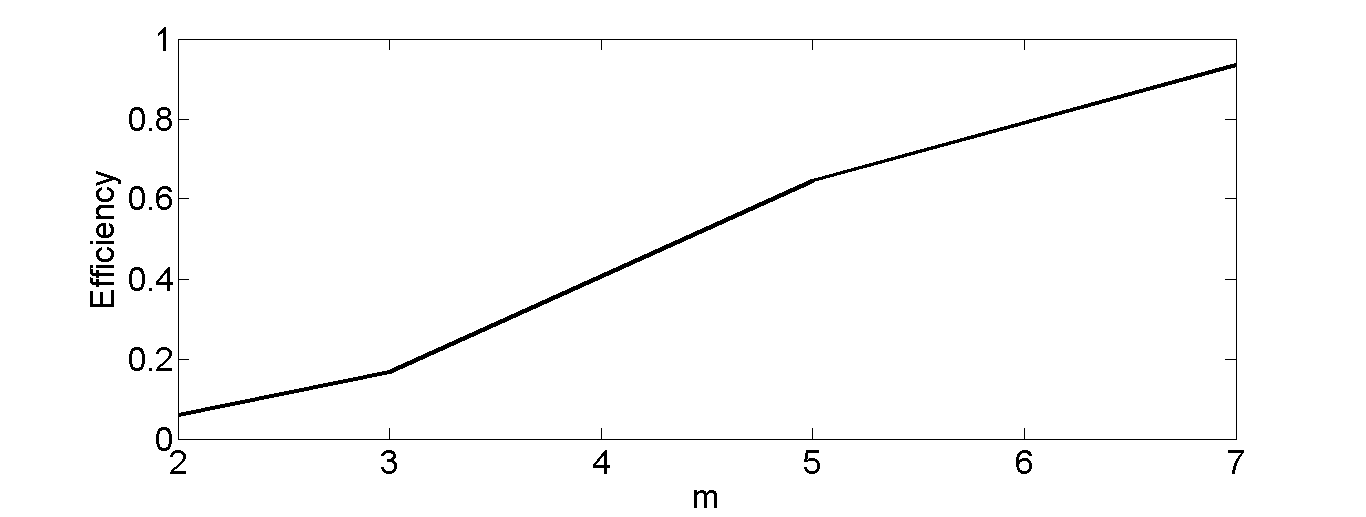
VIII Conclusions and Future Work
We have studied a price competition model with the spatial reuse property where each primary selects a price and a set of non-interfering locations depending on the quality of its channel. We have considered two settings. In the first setting, we consider that the channel state is the same across the networks. We have shown that there exists a symmetric NE strategy profile in the class of mean valid graphs and we have computed a storage and computational efficient NE. The NE strategy profile can be readily implemented as primaries need not communicate with each other even when the NE strategy is not unique. We show that the symmetric NE strategy profile is unique in a linear conflict graph.
In the second setting, we allow that the channel state can be different at different locations. The above consideration significantly complicates the analysis as we have discussed in Section V-A. We, therefore, consider that the channel is either available or unavailable at each node. We have shown that there exists a symmetric NE strategy profile in the class of node symmetric graphs. In order to obtain the symmetric NE strategy, a primary only needs to enumerate the maximum independent sets. The NE strategy is also easy to implement. We have shown that symmetric NE strategy may not be unique in a linear conflict graph in contrast to the first setting.
The characterization of an NE in the second setting where the available channel may belong to multiple states remains open. The analytical results and tools that we have provided in this paper may provide the basis for developing a framework for this problem.
References
- [1] A. Ghosh and S. Sarkar, “Quality sensitive price competition in spectrum oligopoly over multiple locations,” in Information Sciences and Systems (CISS), 2014 48th Annual Conference on. IEEE.
- [2] D. West, Introduction to Graph Theory. 2nd Edition, Prentice Hall, 2000.
- [3] A. Ghosh and S. Sarkar, “Quality sensitive price competition in spectrum oligopoly,” in Proceedings of IEEE International Symposium on Information Theory (ISIT), 2013, pp. 2770–2774.
- [4] A. Ghosh, and S. Sarkar “ Quality-Sensitive Price Competition in Secondary Market Spectrum Oligopoly-Single Location Game,” to appear in Networking, IEEE/ACM Transactions on, 2015. [Online]. Available: 10.1109/TNET.2015.2440422
- [5] G. Kasbekar and S. Sarkar, “Spectrum Pricing Game with Bandwidth Uncertainty and Spatial Reuse in Cognitive Radio Network,” IEEE Journal on Special Areas in Communication, vol. 30, no. 1, pp. 153–164, 2012.
- [6] G. Sabidussi, “Vertex-transitive graphs,” Monatshefte für Mathematik, vol. 68, no. 5, pp. 426–438, 1964.
- [7] E. Weisstein, “Lattice graphs,” 26th June, 2015. [Online]. Available: http://mathworld.wolfram.com/LatticeGraph.html
- [8] A. Mas Colell, M. Whinston, and J. Green, Microeconomic Theory. Oxford University Press, 1995.
- [9] M. Osborne and C. Pitchik, “Price Competition in a Capacity Constrained Duopoly,” Journal On Economic Theory, vol. 38, no. 2, pp. 238–260, 1986.
- [10] D. Kreps and J. Scheinkman, “Quantity Precommitment and Bertrand Competition yield Cournot Outcomes,” Bell Journal of Economics, vol. 14, pp. 326–337, Autumn, 1983.
- [11] O. Ileri, D. Samardzija, T. Sizer, and N. B. Mandayam, “Demand Responsive Pricing and Competitive Spectrum Allocation via a Spectrum Policy Server,” in IEEE Proceedings of DySpan, 2005, pp. 194–202.
- [12] P. Maille and B. Tuffin, “Price War with Partial Spectrum Sharing for Competitive Wireless Service Provider,” in Proceeding Of IEEE GLOBECOM, 2009, pp. 1–6.
- [13] ——, “Analysis Of Price Competition in a Slotted Resource Allocation Game,” in Proceeding of 27th IEEE INFOCOM, 2008, pp. 888–896.
- [14] Y. Xing, R. Chandramouli, and C. Cordeiro, “Price Dynamics in Competitive Agile Spectrum Access Markets,” IEEE Journal on Special Areas in Communication, vol. 25, no. 3, pp. 613–621, 2008.
- [15] D. Niyato and E. Hossain, “Competitive Pricing for Spectrum Sharing in Cognitive Radio Network: Dynamic Games, Inefficiency of Nash Equilibrium, and Collusion,” IEEE Journal on Special Areas in Communication, vol. 26, no. 1, pp. 192–202, 2008.
- [16] D. Niyato, E. Hossain, and Z. Han, “Dynamics of Multiple Seller and Multiple Buyer Spectrum Trading in Cognitive Radio Network: A Game theoretic Modeling approach,” IEEE Transaction on Mobile Computing, vol. 8, no. 8, pp. 1009–1022, 2009.
- [17] X. Zhou and H. Zheng, “TRUST: A General Framework for Truthful Double Spectrum Auctions,” in In the Proceedings of Infocom, April 2009.
- [18] A. M. Kavurmacioglu, E. and D. Starobinski, “Competition in secondary spectrum markets: Price war or market sharing?” in IEEE Proceedings of DYSPAN.
- [19] Y. Tan, S. Sengupta, and K. Subbalakshmi, “Competitive spectrum trading in dynamic spectrum access markets: A price war,” in Global Telecommunications Conference (GLOBECOM 2010), 2010 IEEE, Dec 2010, pp. 1–5.
- [20] L. Duan, J. Huang, and B. Shou, “Competition with dynamic spectrum leasing,” in New Frontiers in Dynamic Spectrum, 2010 IEEE Symposium on, April 2010, pp. 1–11.
- [21] F. Zhang and W. Zhang, “Competition between wireless service providers: Pricing, equilibrium and efficiency,” in Modeling Optimization in Mobile, Ad Hoc Wireless Networks (WiOpt), 2013 11th International Symposium on, May 2013, pp. 208–215.
- [22] J. Jia and Q. Zhang, “Bandwidth and price competitions of wireless service providers in two-stage spectrum market,” in Communications, 2008. ICC ’08. IEEE International Conference on, May 2008, pp. 4953–4957.
- [23] L. Yang, H. Kim, J. Zhang, M. Chiang, and C. wei Tan, “Pricing-based spectrum access control in cognitive radio networks with random access,” in INFOCOM, 2011 Proceedings IEEE, April 2011, pp. 2228–2236.
- [24] S. Sengupta and M. Chatterjee, “An economic framework for dynamic spectrum access and service pricing,” Networking, IEEE/ACM Transactions on, vol. 17, no. 4, pp. 1200–1213, Aug 2009.
- [25] H. Kim, J. Choi, and K. Shin, “Wi-fi 2.0: Price and quality competitions of duopoly cognitive radio wireless service providers with time-varying spectrum availability,” in INFOCOM, 2011 Proceedings IEEE, April 2011, pp. 2453–2461.
- [26] T. M. Cover and J. A. Thomas, Elements of Information Theory, 2nd ed. Wiley, 2006.
- [27] J. G. Proakis and M. Salehi, Digital Communications. McGraw Hill, 5th edition, 2008.
- [28] P. Gupta and P. Kumar, “The capacity of wireless networks,” Information Theory, IEEE Transactions on, vol. 46, no. 2, pp. 388–404, Mar 2000.
- [29] C. Joo, X. Lin, and N. Shroff, “Understanding the capacity region of the greedy maximal scheduling algorithm in multi-hop wireless networks,” in INFOCOM 2008. The 27th Conference on Computer Communications. IEEE, April 2008. (Best paper award).
- [30] A. Gupta, X. Lin, and R. Srikant, “Low-complexity distributed scheduling algorithms for wireless networks,” Networking, IEEE/ACM Transactions on.
- [31] M. I. D. W. Matula, “A 6-regular torus graph family with applications to cellular and interconnection networks,” Graph Algorithms and Applications 3, pp. 373–404, 2004.
- [32] T. E. Harris, “The theory of branching processes,” 1964.
- [33] A. Ghosh and S. Sarkar, “Quality sensitive price competition in spectrum oligopoly: Part ii,” CoRR, vol. abs/1404.6766, 2014.
- [34] S. Z. Li, Markov random field modeling in computer vision. Springer Science & Business Media, 2012.
We prove Theorem 3 (Section IV-E) in Appendix -A. Subsequently, we show Theorem 4 (Section IV-E) in Appendix -B. We show Lemmas 9 and 10 used in Section IV-G to prove Theorem 5 in Appendix -C. We show Theorem 6 (Section IV-G) in Appendix -D. We prove Lemmas 13 and 14 (Section V-B) in Section -E. Finally, in Appendix -F we provide a formal definition of Markov Random Field and show that Markov random field modeling of correlated channel states satisfy Assumption 3 (Section V-A3) under some additional assumptions which naturally arise in practice.
-A Proof of Theorem 3(Section IV-E)
We proceed in two parts. First, we will prove that there exists a distribution which satisfies (25) and (26). Subsequently, we will prove that such a distribution is the unique one.
Existence: First, we will show that the statement is true for . Now, let and . We will show that if then
| (47) |
has a unique solution in , which we will denote as . Let, , then
| (48) |
and
| (49) |
As is strictly decreasing and continuous, so is , thus from (48) and (49), there exists a unique solution between 0 and 1, such that . Note that
| (50) |
is strictly decreasing in . Hence, inverse exists and is also continuous as is continuous. But, . Hence, . Thus, is continuous for . For , define . With the above definition and (50) we obtain is continuous function on and thus
| (51) |
Now, let
| (52) |
As is strictly decreasing on for , is strictly decreasing for . Hence, is strictly decreasing for . Also, note that, for . Thus, for , , as , hence for ,
| (53) |
Now, for , , , thus
| (54) |
As are continuous, so is . Thus, from(53), (54) and intermediate value property, there exists a such that and this is unique as is strictly decreasing. Let, . By definition of , for , and for , (by (51)). Since (from (16)) and , thus for and for . Hence, constitute a probability distribution and satisfy the equations (25) and (26), with and . Thus, the result is true for .
Let, the statement be true for , we have to show that the statement is indeed true for . As the statement is true for , thus, there exists unique distribution such that (25) and (26) holds for . The argument will be similar to the case when with finding unique solution to the equation for for and making for . Hence we omit the proof. Thus, the result is true by the principle of mathematical induction.∎
Uniqueness:
We will prove the uniqueness by Induction hypothesis. First, consider the state .
To reach a contradiction, assume that there exists such that , , (respectively, ) for (respectively ) and for some and :
| (55) | ||||
| (56) |
First, suppose , if , then for . But, is a strictly decreasing and one-to-one mapping, thus for and for , which leads to a contradiction.
If , but , then for . As is strictly decreasing function, hence we must have . Now, for . Thus,
The above inequality lea leads to a contradiction. Thus is not possible, by symmetry, is not possible.
Now, suppose , thus . Since is strictly decreasing function, thus
| (57) |
Since , thus
| (58) |
Thus from (55), (56), (58) and (57), . So, for :
Hence, , thus, , which leads to a contradiction. Hence, is not possible, by symmetry, is not possible.
Thus, the result is true for .
Now, assume that the statement is true for states . Since, the statement is true for states , thus , . Hence, ,. From (16), . As , the proof will be similar to the case when state is .
The result follows from the induction hypothesis.∎
-B Proof of Theorem 4(Section IV-E)
In order to prove Theorem 4 we have to show that any independent set selection strategy of the form (25) and (26) is an NE. We can not use results derived in Section IV-D which we derive assuming that the strategy profile is an NE. However, we use Lemma 8, and Corollary 1 that any independent set selection strategy profile of the form (25) and (26) satisfies regardless of whether it is an NE or not. We also use the following result which can be easily seen from from Lemma 8. Since (by Lemma 8), hence from (25), . Thus, from (16) we obtain
| (59) |
Hence, we can write (26) as
| (60) |
Now we state and prove Lemmas 16 and 17 which are satisfied by any strategy profile of the form (25) and (26). We use these results to prove Theorem 4.
Lemma 16.
if
Proof.
We prove the statement using induction argument.
The statement is trivially true for because by (19).
Now, suppose the statement is true for . Then, for any , , we have
| (61) |
Now, let for . Note that and from (19). Thus, from (20),
| (62) | |||
| (63) |
From corollary 1 since . Using (61) for we have , hence from (19)
| (64) |
Now, since thus (the last inequality follows from lemma 8). Hence,using (26) for we obtain
| (65) | ||||
| (66) |
Thus, from (64), (65) and (66), we obtain
Hence, . The result follows from the induction hypothesis. ∎
Remark 5.
Lemma 17.
If ,then for , , where .
Proof.
Let . Thus, , , and . Since by corollary 1, thus , (or ) if . So, it is enough to show that because and thus .
Since , thus by Lemma 8. Thus, , thus (from observation 1) and thus . Thus, from (20)
| (67) |
Since and from (18); hence, from (20)
| (68) |
Since , hence using (60) for state , we obtain
| (69) |
Again using (60) for state and noting that , we obtain
| (70) |
Since is strictly increasing, in order to show that , from (67) and (68) it is sufficient to show the following
| (71) |
Now we are ready to show Theorem 4.
Proof of Theorem 4: We will show that for channel state , probability distribution as described in (25) and (26) for is a best response.
- 1.
First, we will show that under the strategy profile for , at any independent set ,maximum expected payoff is given by (equation (24)) and the maximum value is obtained at each penalty value in the interval at every node of . (Case i)
- 2.
Next, we will show that for any choice of penalty a primary can only attain at most an expected payoff of at any , (Case ii and Case iii).
- 3.
Finally, we will show that if a primary selects any other independent set i.e. apart from then its expected payoff is upper bounded by for any choice of penalty (Case iv).
Case i:At independent set .
In this case . From Theorem 1, Lemma 2 and (18) at a node , , a primary gets a maximum payoff of when the channel state is . Since , hence . Thus,
Thus, the expected payoff that a primary obtains when channel state is , at independent set ,
Hence, payoff at each node of independent set is
| (72) |
From Theorem 1, the best response penalty set is under at node . Thus, for any , payoff is atmost equal to (72). This completes case i.
Case ii: At independent set , where.
Note from Lemma 8 that . Thus, in this case we must have . As , hence this case arises only when . So, we have from Lemma 17.
Now, as from (59) and thus, . Thus, the expected payoff to a primary at , when the channel state is , is . So, any penalty less than will fetch a strictly lower payoff compared to penalty at any node at . Hence, it is enough to show that if a primary chooses penalty in the interval at a node of , then its payoff will be strictly less than .
If then must belong to interval for some , with . Without loss of generality, we can assume that where . From Corollary 1 , since ; thus is a best penalty response for channel state by Theorem 1. The expected payoff to a primary, when it selects penalty at channel state at a node , is given by
| (73) |
where, is the probability of winning, when a primary selects penalty at channel state , at any node .
Since , thus from (72) we obtain for state
| (74) |
Since and from (27), thus . Since probability of winning only depends on the penalty selected by a primary, thus, when a primary selects penalty at node , at channel state , its expected payoff is
| (75) |
Since , thus expected payoff at any node of at channel state is given by (20) and (72)
| (76) |
Again since , thus, at any node of independent set , maximum expected payoff obtained by a primary at channel state is as given in (72). Expected payoff at at channel state is
| (77) |
If , then ; on the other hand if , then by Lemma 17, . Hence, . Also, note that by definition of . Since (as ); hence, at penalty , at channel state and at a node , expected payoff to a primary is
| (78) |
Case iii: .
We have from (60)
| (79) |
Since thus the maximum expected payoff at is upper bounded by by (72). But, expected payoff to a primary at channel state at at any node of is
| (80) |
Since the expected payoff a primary can attain at a node is at most at channel state . Thus, a primary’s expected payoff at any node is always upper bounded by
| (81) |
Case iv: At any independent set other than :
From (72), (78) and (81), at any node at independent set , we obtain that maximum expected payoff a primary can obtain for state -
| (82) |
The graph we have considered, is a d-partite graph (Section IV-B) . Now, consider an independent set which contains number of nodes from . Then at channel state , expected payoff at independent set is sum of all payoffs at all the nodes contained in . Hence, from (82)
| Expected Payoff at | |||
Thus, at any independent set , expected payoff to a primary at channel state is at most for any selection of penalty. From case (i) a primary attains at following the strategy profile. Hence, the result follows. ∎
-C Proof of Lemmas 9 and 10
Throughout this section we use and ( and respv.) interchangeably.
-C1 Proof of Lemma 9
First we show that .
Let . Without loss of generality assume that . Let consists of number of nodes from . Then
| (83) |
which contradicts (12).
Suppose that for some smallest index . Without loss of generality, we assume that . By the definition of , for , thus . Note that
| (84) |
We consider two possible scenarios:
Case i: does not contain node from .
Since , thus, must consist of nodes of only . Let consist of nodes of . Then,
| (85) |
which is not possible by (12).
Case ii: contains at least one node from for some .
Let consist of number of nodes from . Since , thus, for any and . By (12) for each we have
| (86) |
Since s are disjoint, thus, . Thus, . Hence,
| (87) |
Since contains at least one node from , thus, the above expression is strictly positive. Note that
| (88) |
which contradicts (86), hence this case can not arise. Hence, the result follows. ∎
-C2 Proof of Lemma 10
Let the lowest index be such that but . Thus, contains at least one node from . Without loss of generality we can assume that .
Since for all by Lemma 9, thus, . Let . Let consists of number of nodes from . Thus,
| (89) |
Note that LHS of (89) is always non-negative. Now, we will show that (89) is strictly positive. If it is not strictly positive then we must have
| (90) |
But RHS of (90) is equal to
| (91) |
and LHS of (90) is equal to
| (92) |
Thus,
| (93) |
But contains at least one node from and . Thus, contains at least one node in common with which is not possible since s are disjoint. Thus (89) is strictly positive. Thus, there must exist a such that contains at least one node from . Since and , thus, . Hence, we have found a such that contains at least one node from such that which contradicts the definition of . Hence, the result follows.∎
-D Proof of Theorem 6 (Section IV-G)
In order to prove Theorem 6 we must consider all symmetric NE strategy profiles which need not be of the form (14); this precludes the use of the results in section IV-D. First, we characterize some properties that any symmetric NE strategy must follow (Lemmas 19, 21) in Appendix -D1. Then we deduce some important properties (Lemma 23 and 24) that any NE strategy profile must satisfy in a linear graph in Appendix -D2. We then use those properties to prove Theorem 6.
-D1 Properties of any symmetric NE strategy profile (Lemmas 19 and 21)
In order to prove Lemma 19 we state and prove Observations 4, and 5 and Lemma18. We subsequently state and prove Lemma 20 to prove Lemma 21.
We start with some notations, which we use throughout.
Definition 14.
denotes the maximum expected payoff under an NE strategy for state at node 1616 16 Even if node is selected with probability when the channel state is , we can still defined as the maximum expected payoff that a primary would have obtained if it would select node .
Recall from (9) that the channel is offered at node when the state is with probability . With slight abuse of notation, we define for node in the following manner:
| (94) |
Thus, denotes the probability that the channel is offered at node when the state is higher or equal to .
Since we have to consider all NE strategy profiles which may not be of the form (14), thus, the payoff, upper and lower endpoint need not be the identical at each node of at a given channel state. By Lemma 2 if is known then the above parameters can be obtained using Lemma 1 with in place of . With slight abuse of notation we denote and for node i.e. for
| (95) | |||||
| (96) |
By Theorem 1 is the expected payoff at node when the channel state is if node is selected with positive probability. By Theorem 1 a primary selected penalty from the interval when the channel state is using the distribution (4) with in place of .
Now we state some observations which we use throughout.
Observation 4.
At node , where .
Observation 4 readily follows from (94). Since from (94)
Similar to observation 2, using observation 4, (96) and (95) we obtain
Observation 5.
At node , for iff . iff . Hence, iff .
Lemma 18.
Maximum expected payoff under the NE strategy profile at a node is obtained at when channel states are and . When the channel state is , primary attains its maximum expected payoff at at any node.
Note that if then by Theorem 1 is a best penalty response at channel state . Here we show that even if , then the maximum expected payoff is obtained at at node under any NE strategy profile.
Proof.
First, we will prove the statement for channel state . The proof for channel state will readily follow.
Suppose the statement is false for channel state . Hence, there exists at which expected payoff is higher compared to the expected payoff at when the channel state is . First we rule out (case i) and then (case ii).
case i: :
Note that this case can not arise when . Hence, ; thus by observation 5 there must exist such that . If , then ; on the other hand if then by observation 5 . Expected payoff to a primary at state at is
| (97) |
where is the probability of winning at penalty at node . By theorem 1, is a best penalty response at node when the channel state is . Now, expected payoff at when channel state is , is
Note that players with channel state higher than select a penalty lower than or equal to with probability and players with channel state lower than or equal to select a penalty lower than or equal to with probability at node . Thus, the expected payoff to a primary when it selects penalty at channel state at node is
| (98) |
Note that by (96).
Since expected payoff at is strictly higher compared to the expected payoff at at node at channel state and , thus, we have from (97) and (98)
| (99) |
On the other hand, the expected payoff that a primary will obtain when it selects penalty at node at channel state -
| (100) |
which contradicts the fact that is a best penalty response at channel state .
Case ii :
Note that, if forall , then it is trivial that this case can not arise1717
17
In this case, (by observation 5) for all . Thus, expected payoff at any penalty strictly less than at will yield strictly lower payoff compared to payoff at . We only consider the scenario when for some . Note that . Now let, . By definition of and observation 5 . Since , thus expected payoff at is the maximum expected payoff at node when the channel state is (theorem 1). Expected payoff to a primary channel state at is
where denotes the probability of winning when a primary offers penalty at node . Since probability of winning does not depend on the channel state, hence, expected payoff to a primary at channel state and at penalty is
| (101) |
Let, probability of winning at penalty at node be . Since, probability of winning does not depend on the channel state , thus expected payoff to a primary when it offers penalty at channel state and at node is
Similarly expected payoff at node , at channel state and at penalty is-
Since is a best penalty response to channel state at node , thus
| (102) |
From (101), expected payoff at at node and at channel state is given by
| (103) |
which contradicts the fact that expected payoff at is higher compared to the expected payoff at when the channel state is .
Now, we show the result for channel state .
If , then by observation 5 . Hence, the same analysis will follow for channel state . On the other hand if which along with (by (96) implies that is the upper endpoint of the penalty selection strategy profile for channel state at node . Since the upper endpoint is also a best penalty response by theorem 1, thus the result follows. ∎
Since is a best response at channel state at any node in the network by Lemma 18, thus,
| (104) |
By (96) expected payoff at is
| (105) | |||
| (106) |
Lemma 19.
i) For, , if and , then .
ii) If and , , then .
Proof.
First we show part (i). Proof of part (ii) follows by simple modification of the proof of part (i).
Suppose, the statement is false, i.e. for some and . As thus,
| (107) |
Now, as , hence from (106)
| (108) |
Since (from (107)) is strictly decreasing, thus . Since is strictly increasing, thus we obtain from (108) . Now, from (108) and the fact that , we obtain
which contradicts the fact that .
Note that, if and , then we also obtain (107) by simple algebraic manipulation, hence the proof of part (ii) is exactly similar to the proof of part (i). ∎
We use the following result in proving lemma 21.
Lemma 20.
Suppose . Let, , then such that , we must have .
Proof.
Suppose the statement is false. So, there exists a such that , 1818 18 Note that the statement is true at state , since . Since , thus, there must exist a , such that but . Because otherwise we have .
Since , thus from observation 4
| (109) |
By definition of , for , since and , thus . Hence, from (109), we have .
But and , hence by lemma 19 we have which leads to a contradiction. ∎
Lemma 21.
Suppose, , then there must exist a state such that but .
Proof.
First we show that the statement is true when (case i) and then we show when (case ii); which completes the proof.
Case 1: Suppose . Since, is strictly decreasing, thus from (104) we obtain . Thus, from (94), there must exist . By lemma 20, such that . Since at , , thus, the statement is true for .
-D2 Properties of any symmetric NE strategy profile in a linear graph (lemmas 23 and 24)
We consider a linear graph (fig. 1) consisting of number of nodes. We use the properties of linear graph and a NE strategy profile to prove the results. First, we state and prove Lemma 22. Subsequently, we show that under an NE strategy profile the maximum expected payoff to a primary at a channel state at each node of must be equal (Lemma 23). Then, we show that under an NE strategy profile nodes of are selected with equal probability (Lemma 24). Finally, we show theorem 6 using lemmas 23 and 24.
In order to prove Lemma 22 we state and prove Observations 6,7,and 8.
Observation 6.
An NE independent set selection strategy profile only selects a maximal independent set with positive probability.
Proof.
Suppose not; so an independent set has been chosen with positive probability under an NE strategy profile, but it is not maximal which in turn implies that there exists a node , such that is an independent set. Since (from (10)), hence at node , primary will attain at least a payoff of for state when the primary selects the highest possible penalty . Hence, a primary can attain strictly higher payoff by choosing independent set compared to . Hence, the result follows. ∎
Observation 6 enables us to focus only on the maximal independent sets for an NE strategy profile.
Observation 7.
For a maximal independent set -
(i) If , but , then for some .
(ii) If , but , then for some .
Proof.
part (i): If it is not then is maximal, since (as and is an independent set); which contradicts that is maximal.
part (ii): If it is not then is an independent set since which contradicts that is maximal. ∎
Observation 8.
Consider an independent set , such that , but , for some ; NE independent selection strategy profile selects with positive probability, the following condition must be satisfied for
| (113) |
Proof.
Note that if , then does not contain node , hence is not maximal. Thus, an NE strategy profile can not select by Observation 6. Hence, we must have .
If , then we can replace node with node and we obtain an independent set as . But, we can get strictly higher payoff at the independent set , as all the nodes are same except and . This contradicts that NE strategy profile selects with positive probability.
Similarly if then we obtain an independent set by replacing node with in and can get a strictly higher payoff at that independent set. ∎
Lemma 22.
i) If , then for some .
ii)If , then for some .
Proof.
We prove (i). The proof of (ii) will be similar to the proof of part (i) by symmetry.
Since , hence, from Lemma 21, there exists such that , but . Hence, there must exist a maximal independent set such that , but , which is chosen with positive probability in an NE strategy profile when the channel state is . But, as is maximal, thus, from Observation 7. Also from Observation 8, we must have
| (114) |
Since , thus, from (114), we obtain
Hence, we obtain for some only using the fact that .Thus, by recurrence on the index we obtain the result. ∎
Next Lemma characterizes that under an NE strategy profile maximum expected payoff must be equal at every node of .
Lemma 23.
Under NE strategy profile, we must have
| (115) |
Proof.
First, we prove , .
We show that ; by symmetry we get . Suppose, for some . Then, there must exist a maximal independent set such that node , but node ; which is not possible (figure 1).
Now, we are ready to prove the lemma.
Suppose the statement is false. So, we must have for some and . We rule out , by symmetry it follows that ; which completes the proof.
Next, lemma shows that under an NE strategy profile nodes in are selected with equal probability.
Lemma 24.
For state , where .
Proof.
Let, be the lowest channel state, for which the statement is false. Thus, there must exist node such that, , but (by Lemma 23). First we rule out that (case i) and then (case ii).
Proof of Theorem 6: First, we will show that for any NE strategy profile we must have . Then, we will show that if a primary chooses a maximal independent set other than and with positive probability, then we must have , which completes the proof.
Suppose but it is an NE for some . Since and constitute a partition of , thus, the expected payoff that any primary at channel state will get is the following
| (117) |
Consider the following unilateral deviation for primary 1 at channel state : Primary 1 chooses with probability and with probability . Since remains the same, is strictly positive, and , hence primary 1 gets a strictly higher payoff following the above mentioned strategy by (117). This contradicts that is an NE distribution.
Next, consider an NE strategy profile which selects a maximal independent set , which has at least one node both from and , with positive probability. Hence, there exists a node such that . Since and are adjacent, hence both can not appear in any independent set otherwise can not be an independent set. Hence, by valid distribution property, we must have
| (118) |
On the other hand for independent set , both . Since is chosen with positive probability, hence from (118)
| (119) |
Without loss of generality, we can assume that , hence . Thus, and . We have already shown that for any NE strategy profile we must have which contradicts (119). Hence, a primary can not choose an independent set which contains at least one node from and under an NE strategy; since and constitute a partition of ; thus, only subsets of either or can be selected with positive probability. Since proper subsets of either or are not maximal, they can not be chosen with positive probability under an NE strategy by Observation 6. Hence, the result follows.∎
-E Proof of Lemmas 13 and 14 (Section V-B)
-E1 Proof of Lemma 13
:In order to prove Lemma 13 first, we describe an infinite set of strategy profile . Subsequently, we show that every strategy profile in is an NE.
Note that at a channel state vector , a linear graph consists of disjoint smaller linear graphs (Fig. 19). First, we introduce some notations. Let be the linear graph which starts from node i.e. the channel is not available at node if (fig. 19), but it is available at node .
In the two maximal independent sets which partition the set of nodes in are: which contains the nodes numbered and which contains the nodes numbered . In figure 19, and constitute two disconnected linear graphs. The cardinality of can be an even or odd number depending on the number of consecutive nodes where the channel is available starting from node . To illustrate the cardinalities of , consider the linear graph with nodes. Here, can take any value in . When , then the channel is available at node but not at node . When , then the channel is available at node and , but the channel is not available at node . Here and . When , then the channel is available at nodes , but the channel is unavailable at node . Here, and . When , the channel of the primary is available at all nodes. Thus, coincides with and coincides with where and .

Since for a given channel state vector , the graph can be partitioned into linear graphs (fig. 19), thus, a primary only needs to select strategy for each such linear graph. Thus,
Lemma 25.
Obtaining an NE strategy profile is equivalent to obtain an NE strategy at each possible mean valid graph , .
We use the following result to prove Theorem 13.
Observation 9.
When is odd, then the only maximum independent set is , if is even, then both and are maximum independent sets of .
Note that when is even, there can be other maximum independent sets apart from and 1919 19 For example, when , then, the following are maximum independent sets, , , and where the first two independent sets belong to and respectively.
Now, we consider a linear graph with nodes and the channel states are I.I.D. i.e. the channel is at state at a given node is w.p. . Let denote the probability of the event that . It is easy to show the following
| (120) |
| (121) |
| (122) |
| (123) |
Now, we describe an uncountable set of strategy profiles parameterized by parameters and .
Strategy profile : If is odd, then will be selected w.p. . If , then will be selected w.p. and will be selected w.p. . If i.e. when the channel is available at all nodes, then will be selected w.p. and will be selected w.p. . If , then will be selected w.p. and will be selected w.p. . If , then will be selected w.p. and will be selected w.p. .
where are such that
| (124) |
Since and , thus, it is easy to discern that the strategy profile described in constitutes a valid distribution. Note that there are uncountably infinite numbers of satisfying (124). Thus, gives rise an infinite number of strategies.
Towards this end we first show that under the strategy profile the channel is offered by a primary at every node with the same probability.
Node selection probability of node i.e. is
| (125) |
and node selection probability of node is
| (126) |
Node selection probability of node i.e. is
| (127) |
Node selection probability of node is
| (128) |
Note that
| (129) |
Thus, from (125) and (126), we obtain that is equal to
| (130) |
Note that by (120) and by (123). Since from (122), thus it readily follows from (130) that . From (127) and (126) we obtain is equal to
| (131) |
Note that by (120), and by (121). Thus, from (131)
| (132) |
Also note from (122) that . Thus, . Thus, from (129) and (132) it readily follows that . From (127) and (128) we obtain that is equal to
| (133) |
Note that by (120). Also note that by (123). Thus, from
| (134) |
Since by (122), thus, we obtain . Since by (121), thus, from (129) and (134) it readily follows that . Hence, we obtain .
Since node selection probability is identical across the nodes, thus, when all the other primaries select a strategy profile in the set , then, the maximum payoff of primary at a node is by Theorem 1 and (42) and this is obtained for any penalty in the interval with in place of by Lemma 2. Hence, the maximum attainable expected payoff of primary at each location is the same since ’s are identical.
Now, we show that primary does not have any incentive to deviate from a strategy profile for fixed when other primaries also select that strategy profile.
When is odd, then by Observation 9 is the only maximum independent set in . Since the maximum attainable expected payoff for primary is the same at every node, thus, the expected payoff at is the highest for primary when all the other primaries select a strategy profile in . Hence, primary does not have any incentive to deviate from when is odd since under primary selects w.p. when is odd.
When is even, then . By Observation 9 both , are the maximum independent sets. Since the maximum attainable expected payoff is the same at each node, thus, any strategy profile which randomizes between and gives the highest expected payoff to primary . Thus, primary does not have any incentive to deviate from when is even since under primary only randomizes between and .
Though we only consider primary since the every strategy in is symmetric, hence, no primary will have any incentive to deviate unilaterally from the strategy profile for a fixed . Thus, we show that every which satisfy (124), the strategy set in is an NE.
Since there are uncountable number of s which satisfy (124), hence there are multiple NEs in this setting.∎
-E2 Proof of Lemma 14
We show that is not a NE strategy profile in the above linear graph with nodes where the channel is in state at a given location w.p irrespective of the channel states at other locations. In order to prove the result we use some of the results which we derived in the previous section to prove Lemma 13.
First, we point out the how (described in Section V-B) is different from the class of strategy profile (described in the previous section). Then, we show that is not an NE in this setting.
Since and are the only maximum independent sets of when by Observation 9, thus, according to (Section V-B), when , and must be selected w.p . Note that in when , is selected w.p. , and is selected w.p. where . Thus, and are not selected with equal probabilities even though they are of same sizes. Thus, does not belong to . Now we show that can not be an NE.
puts equal weight on every maximum independent sets. When , then under , each of the maximum independent sets and with equal probabilities. Hence, the channel is offered at node w.p. when . Thus, under , the node selection probability is
| (135) |
and node selection probability of node is
| (136) |
Now, we show that . Since (by (120)) and , thus, we are left to show that . By simple algebraic calculation for , we have . Hence . Thus, .
Thus, by the single location pricing strategy the maximum expected payoff attained by a primary at node is (from (42)) and the expected payoff attained by a primary at node is ( by (42)) when the other primaries select . Since and is strictly increasing, thus, the expected payoff at node is strictly higher compared to the node . Thus, when , if a primary selects node w.p. , then it would attain strictly higher payoff compared to the strategy where a primary selects node w.p. and node w.p. when . Hence, a primary has an incentive to deviate unilaterally from its strategy profile. Hence, is not an NE.∎
-F Markov Random Field
-F1 Background
A Markov random field is a graphical model which represents the joint probability distributions of random variables having Markov property. It is represented by an undirected graph in which the nodes represents the random variables. The edges encodes the dependencies among the random variables in the following way: if is the set of neighbors of , then in a Markov random field[34],
Figure 21 provides a cyclic Markov random field. Here, .


The channel states in a conflict graph are random variables whose values are either or . Since the channel states at adjacent locations are likely to be correlated, we model the correlation amongst the adjacent locations in the conflict graph using the Markov Random field where the nodes in the Markov random field represent the channel states of the corresponding nodes of conflict graph . Figure 21 represents a Markov random field when the conflict graph is a cyclic graph with nodes and the values of the random variables represent the channel states at nodes of conflict graph respectively.
We now discuss the joint probability distribution in the Markov random field. Markov random fields provide a compact representation of the joint probability distribution in terms of product of potential functions. Potential functions are defined on the set of maximal cliques, , in the graphical representation of the Markov random field . A potential function represent the values of the random variable of the maximal clique . For example, in figure 21 the set is a maximal clique, thus, denote the value of the potential function when the random variables and , . Note that is defined on the vector which represents the values of the random variables represented by nodes in the clique . Formally, the probability of the channel state is given by:
| (137) |
where is a normalization factor and denote the channel states in clique when the overall channel state vector is .
For example, in figure 21 the set of maximal cliques is . The joint probability distribution is given by
Since only take values in , we can represent as a matrix where denote the value of the th position of the matrix. For example, can be the following:
| (138) |
In Figure 21, the maximal cliques are . Hence, the joint probability distributions are
| (139) |
Definition 15.
The Markov random field representation of random variables is symmetric if i) the maximal cliques are of identical sizes and ii) suppose corresponds to the channel state vector of maximal clique and corresponds to the channel state vector of maximal clique , then
| (140) |
for every and such that and contain the same number of s (and thus, the same number of s since are of same sizes).
(138) provides an example of potential functions which are symmetric and identical. But potential functions in Fig. 21 can not be symmetric since the sizes of the maximal cliques are different.
Now, we are ready to provide an example which satisfies Assumption 3.
-F2 Result
Lemma 26.
The probability distributions on the channel states satisfy Assumption 3 if
i) The channel states constitute a Markov random field,
ii) The graphical representation of the Markov random field is the same as the node symmetric graph ,
iii) The Markov random field relation is symmetric2020
20
In a node symmetric graph, the maximal cliques are of the same size, and
iv) There are fixed integers such that every clique containing number of nodes is a subset of identical () number of maximal cliques in .
First, it is easy to discern that the condition (iv) is satisfied by a large class of node symmetric conflict graphs including cyclic graph, infinite linear graph (Fig. 11), infinite square graph(Fig. 14), infinite grid graph (Fig. 14), infinite triangular graph (Fig. 14). For example, in the infinite triangular graph (Fig. 22), a clique containing nodes is a maximal clique and hence, it is a part of only maximal clique; any clique containing nodes is a subset of maximal cliques; a single node is a part of maximal cliques.

In order to prove the above lemma, we first show the following for any node symmetric graph which satisfies condition (iv):
Observation 10.
Let be the number of maximal cliques in which contains exactly nodes of , then there are exactly number of maximal cliques in which contains exactly nodes of , when is isomorphic to .
Proof.
Let and be isomorphic (Definition 12) to each other, where and are the conflict graphs corresponding to the channel state vectors and respectively. Since and are isomorphic, there is an isomorphic function between the nodes of and .
Suppose that there is a maximal clique which contains nodes of . Thus, this set of nodes is a subset of a maximal clique. The isomorphic function maps those nodes into different nodes of . Also note that since these nodes of belong to a clique in the original graph , hence they are adjacent to each other, since is isomorphic, thus, the mapped nodes must also be adjacent to each other, hence that set of mapped nodes is also a subset of a maximal clique in the original graph .
Suppose the statement in the result is false. Thus, there must exist a set of nodes of which is a subset of number of maximal cliques in the original graph, however the mapped set of nodes of is only a subset of number of maximal cliques in the original graph where . Thus, this violates the condition (iv). Hence, . By symmetry, we can also show that the situation where can not arise. Hence, the result follows. ∎
Now, we are ready to prove Lemma 26.
Proof.
Let and be isomorphic to each other, where and are the conflict graphs corresponding to the channel state vectors and respectively. We have to show that . Let be the channel state vector at the nodes of when the channel state vector is .
Now, at channel state vector , the potential function value at maximal clique is . Thus, the channel state vector and are given by
| (141) |
By Observation 10, the number of maximal cliques which contain number of nodes of and are identical. Note that at channel state vectors and , the nodes where the channel state is are only the nodes of and respectively. Hence, the number of maximal cliques which contain exactly number of s are the same (and thus, the number of s since in the node symmetric graph, the size of maximal cliques are the same) in the channel state vectors and . Hence, from (140) and (141). ∎