A Comparison of First-order Algorithms for Machine Learning

Fobos [5] and fast iterative shrinkage-thresholding algorithm [1] (FISTA) aim to solve a convex problem which is a sum of two convex functions. Neumaier [7] proposes a fast subgradient algorithm with optimal complexity for minimizing a convex function named optimal subgradient algorithm (OSGA). Chambolle and Pock [3] propose a primal-dual algorithm (hereinafter referred as PD CP) and applied it to several imaging problems. Tianbao Yang et al. [10] propose another primal-dual algorithm and applied it to machine learning tasks. However, PD CP is more general in the following aspects. The step size of PD CP is $\sqrt{2}$ times larger than [10] and PD CP makes steps in both primal and dual variables.

We summarize four solvers by Table  1. Each solver can achieve the convergence rate under the property of $F,G,E$ given by each row of Table  1. When we solve machine learning problems using four solvers, we need to set the value of parameters and format the machine learning problems to a suitable model for a solver. Setting the initial step size C in Fobos for a problem with non-smooth function is an open question. For PD CP, we do not know the best ratio $a=\sqrt{\tau/\sigma}$. When solving a problem with a non-smooth function by FISTA, we have to smooth the non-smooth loss function. This rises a problem of selecting the value of smoothness parameter $\epsilon$ in smoothing techniques. To make the comparison convincing, we examine several values for the above three parameters $C,a,\epsilon$ and choose the best one.

In this section, we review the primal dual algorithm proposed in [3]. Let $X,Y$ be two finite dimensional real vector spaces with an inner product $\left\langle\cdot,\cdot\right\rangle$ and norm $\left\lVert\cdot\right\rVert=\left\langle\cdot,\cdot\right\rangle^{\frac{1}{2}}$. The map $K:X\rightarrow Y$ is a continuous linear operator with induced norm

PD CP is to solve the generic saddle-point problem

where $x$ is the primal variable and $y$ is the dual variable. $G$ and $F^{*}$ both are proper convex, lower-semicontinuous functions. The primal form of  Equation (1) is $\min\limits_{x\in X}F(Kx)+G(x)$. To introduce the dual variable y, one way is using Lagrange multipliers, e.g., applicable when the function represents hard constraints. The other way is to calculate the convex conjugate $F^{*}$ of loss function $F$. Then the loss function can be expressed by its convex conjugate. Take the hinge loss for example. We simplify the definition of hinge loss as $f(z)=\left\lVert\max(0,z)\right\rVert_{1},z\in\mathbb{R}^{N}$. Its convex conjugate is,

where $P=\left\{y\in\mathbb{R}^{N}:\forall y_{i}\in\left[0,1\right]\right\}$, $y_{i}$ is the $i^{th}$ component of $y$. Let $z=1-Kx,x\in\mathbb{R}^{d}$ and $K\in\mathbb{R}^{N\times d}$. Then according to $f(z)=\max\limits_{y}\left\langle z,y\right\rangle-f^{*}(y)$, $f(1-Kx)$ can be defined as,

Therefore in the primal-dual model, $F^{*}$ should be formulated as $-\sum\limits_{i=1}^{N}y_{i}+f^{*}(y)$.

Before summarizing PD CP, we introduce the proximal operator. Let $G:\ X\rightarrow\mathbb{R}\cup\left\{+\infty\right\}$ be a proper convex, lower-semicontinuous function. The proximal operator of $G$ with parameter $\tau$ is defined by

Since Euclidean norm is strong convex, $\mathrm{prox}_{\tau G}(v)$ is unique. PD CP proceeds by iteratively maximizing with respect to the dual variable and minimizing with respect to the primal variable by proximal operators.

Now we summarize PD CP as follows,

$\bullet$ Initialization: $\tau\sigma\leq\frac{1}{\left\lVert K\right\rVert^{2}}$,$\theta\in\left[0,1\right]$,$(x^{0},y^{0})\in X\times Y$,$\overline{x}^{0}=x^{0},\lambda\in\mathbb{R}$ $\bullet$ Iterations $n\geq 0$: Update $x^{n},y^{n}$ as follows, $\displaystyle y^{n+1}$ $\displaystyle=(I+\sigma\partial F^{*})^{-1}(y^{n}+\sigma K\overline{x}^{n})$ (4) $\displaystyle x^{n+1}$ $\displaystyle=(I+\tau\lambda\partial G)^{-1}({x}^{n}-\tau K^{*}y^{n+1})$ (5) $\displaystyle\overline{x}^{n+1}$ $\displaystyle=x^{n+1}+\theta(x^{n+1}-x^{n})$ (6)

PD CP conducts proximal operators of $\sigma F^{*}$ and $\tau\lambda G$ respectively and then PD CP makes its scheme semi-implicit by letting $\overline{x}^{n+1}=x^{n+1}+\theta(x^{n+1}-x^{n})$. This operation equals to making one more step in the direction of $x^{n+1}-x^{n}$. We refer to [3] for more information. The condition of the convergence of PD CP is $\tau\sigma\leq\tfrac{1}{\left\lVert K\right\rVert^{2}}$.

In this section, we introduce two heuristic observations of the primal-dual algorithm proposed by Chambolle and Pock [3].

In PD CP, we define $a=\sqrt{\tau/\sigma}$. How to choose $a$ to achieve the best performance is still an unsolved problem. However, Chambolle and Pock [3] show that

where $x_{N}=(\sum\limits_{n=1}^{N}x^{n})/N$, $y_{N}=(\sum\limits_{n=1}^{N}y^{n})/N$ and $(\widehat{x},\widehat{y})$ is the saddle point. The RHS of  Equation (7) is non-negative because

And when $(x_{N},y_{N})$ is a saddle point, the LHS of  Equation (7) equals zero. To minimize the upper bound of $\left[\left\langle Kx_{N},\widehat{y}\right\rangle-F^{*}(\widehat{y})+G(x_{N})\right]-\left[\left\langle K\widehat{x},y_{N}\right\rangle-F^{*}(y_{N})+G(\widehat{x})\right]$, we plug $\tau=\frac{1}{\left\lVert K\right\rVert^{2}\sigma}$, the largest value that guarantees convergence, into the RHS of  Equation (7) and get

Equation (10) is a convex function of $\sigma$. We take the derivative of  Equation (10) with respect to $\sigma$,

Thus we can conclude that $\frac{1}{N}(\frac{\left\lVert\widehat{y}-y^{0}\right\rVert^{2}}{2\sigma}+\frac{\left\lVert\widehat{x}-x^{0}\right\rVert^{2}}{2\tau})$ reaches its minimum when $a=\sqrt{\frac{\tau}{\sigma}}=\frac{\left\lVert\widehat{x}-x^{0}\right\rVert}{\left\lVert\widehat{y}-y^{0}\right\rVert}$. However, $\widehat{x}$ and $\widehat{y}$ are not available because they are what we want to calculate.

We observe that the convergence condition [3] $\tau\sigma\leq\tfrac{1}{\left\lVert K\right\rVert^{2}}$ can be relaxed to accelerate the algorithm. We refer to the resulting scheme as Online PD CP. Although Online PD CP converges in the experiments of this paper, we do not prove its convergence theoretically. Online PD CP try to seek a larger step size. Once it finds one, it is faster than PD CP in the experiments of this paper. The difference between PD CP and Online PD CP is that Online PD CP starts with a larger step size ($\tau\sigma>\frac{1}{\left\lVert K\right\rVert^{2}}$) and decreases it according to a certain rule. We employ the following scheme,

Thus how to choose a proper $L$ is the main concern of Online PD CP. As shown in  Equation (11), we let $L^{n+1}=\max\left(L^{n},\widetilde{L}^{n+1}\right)$. If $L^{n}<\widetilde{L}^{n+1}$, we increase $L^{n+1}$ to $\widetilde{L}^{n+1}$. Thus, $\left\lVert K\right\rVert$ is a upper bound of $L$. Chambolle and Pock [3] proves the convergence when $L=\left\lVert K\right\rVert$.

Another observation is that the larger step size may lead to a large $L$. If $\widetilde{L}^{n+1}$ is smaller than $L^{n}$, Online PD CP does not update $L^{n+1}$. It is a sign of convergence and stability. That is, inappropriate large step sizes lead to divergence and a large $\widetilde{L}$ which may be close to $\left\lVert K\right\rVert$. This obeys the principle of Online PD CP. To explore more possible step sizes, we decrease the step size to an appropriate degree rather than choose the maximum between $L^{n}$ and $\widetilde{L}^{n+1}$. This is the reason that we smooth $L$. We can devise different rules to smooth $L$. For example, we let $L=(L+\kappa\max(L,{L}^{n+1}))/(1+\kappa),\kappa>0$. We set $\kappa=0.618$ for all experiments. The other use of Online PD CP is the case that $\left\lVert K\right\rVert$ is non-calculable, e.g., $K$ is not known explicitly.

When $\nabla F$ is with a Lipschitz constant $L$, the convergence rate of Fobos can be $O(1/n)$ [1]. Thus, we only compare Fobos with FISTA, OSGA and PD CP in the machine learning problems where $F$ and $G$ are both non-smooth. In all experiments, we initialize the primal variable and the dual variable to a null vector. All algorithms were implemented in Matlab and executed on a 2.66 GHz CPU, running a 64 Bit Windows system.

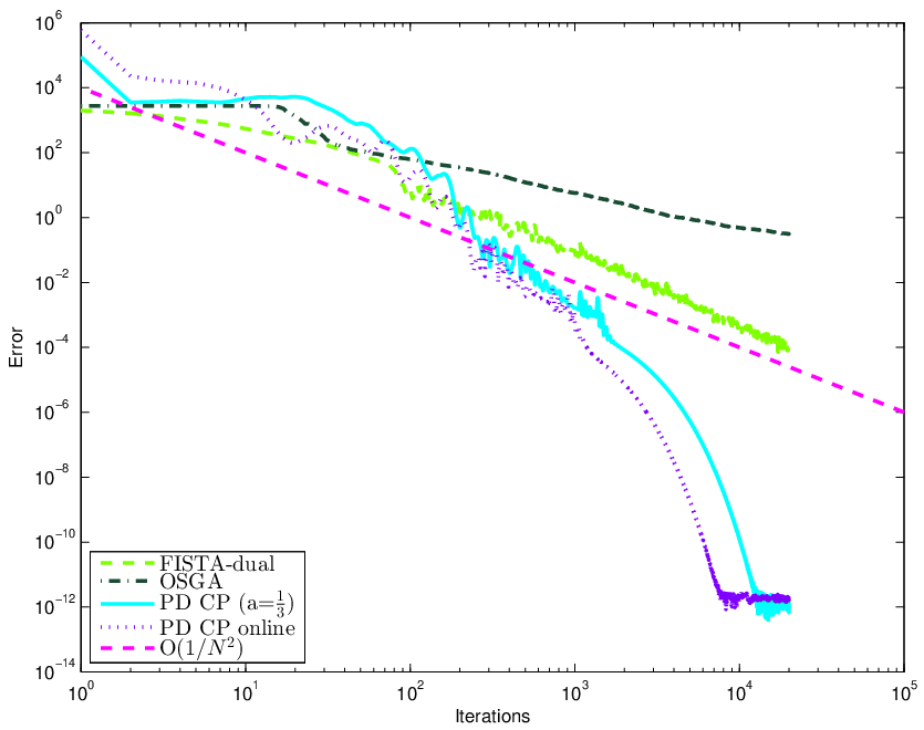
Figure  1 compares the practical convergence rate. During the different ranges of iterations, solvers can have different performances. For example, normally FISTA is faster within the first ten iterations but only reaches the optimal solution in the experiment of dimensionality reduction. When loss function and regularizer are both smooth as in Kernel SVM, FISTA shows exactly convergence rate $O(1/n^{2})$. If we prolong the line of FISTA in Figure  1(c), we can see FISTA needs about $10^{7.8}$ iterations to reach the optimal solution. However, PD CP only needs about $10^{4}$ iterations. For the last three experiments where loss functions and regularizers are both non-smooth, Fobos shows a convergence rate $O(1/\sqrt{n})$. But for all experiments, PD CP is the fastest to reach the optimal solution. Although the performances of PD CP with different values of $a$ are different, they show a similar practical convergence rate as shown in Figure  1(a) and  1(b). PD CP has a much better practical convergence rate which is even better than $O(1/n^{2})$. The experimental results show that FISTA is less capable to handle the case of two non-smooth terms. Furthermore, we may not get the optimal values by FISTA since we use the smoothing techniques. In all experiments, Online PD CP is better than or equal with PD CP. Refer the supplementary material for more results of machine learning problems. From Table  3, we can observe PD CP is still very competitive. Only in Multi-Task Learning, the running time per iteration of PD CP is slower than OSGA’s. However, by observing Figure  1(e), PD CP needs much less number of iterations to approach the optimal solution. Overall, PD CP have the superior performance among all machine learning problems considered in this paper.

References

- [1] Amir Beck and Marc Teboulle. A fast iterative shrinkage-thresholding algorithm for linear inverse problems. SIAM J. Img. Sci., 2(1):183–202, March 2009.
- [2] Kristin P. Bennett and Emilio Parrado-Hernández. The interplay of optimization and machine learning research. J. Mach. Learn. Res., 7:1265–1281, December 2006.
- [3] Antonin Chambolle and Thomas Pock. A first-order primal-dual algorithm for convex problems with applications to imaging. Journal of Mathematical Imaging and Vision, 40(1):120–145, 2011.
- [4] Olivier Chapelle. Training a support vector machine in the primal. Neural Computation, 19:1155–1178, 2007.
- [5] John Duchi and Yoram Singer. Efficient online and batch learning using forward backward splitting. J. Mach. Learn. Res., 10:2899–2934, December 2009.
- [6] Junbin Gao, Qinfeng Shi, and Tibério S. Caetano. Dimensionality reduction via compressive sensing. Pattern Recogn. Lett., 33(9):1163–1170, July 2012.
- [7] Arnold Neumaier. Osga: A fast subgradient algorithm with optimal complexity. Unpublished manuscript, 2014.
- [8] Ofir Pele, Ben Taskar, Amir Globerson, and Michael Werman. The pairwise piecewise-linear embedding for efficient non-linear classification. In ICML, 2013.
- [9] Haiqin Yang, Zenglin Xu, Irwin King, and Michael R. Lyu. Online learning for group lasso. In ICML, 2010.
- [10] Tianbao Yang, Mehrdad Mahdavi, Rong Jin, and Shenghuo Zhu. An efficient primal-dual prox method for non-smooth optimization. Mach Learn, 2014.