Non-Gaussianity after BICEP2
Abstract
We analyze primordial non-Gaussianity in single field inflationary models when the tensor/scalar ratio is large. Our results show that detectable levels of non-Gaussianity are still possible in the simplest class of models described by the effective theory of inflation. However, the shape is very tightly constrained, making a sharp prediction that could be confirmed or falsified by a future detection of non-Gaussianity.
Current cosmological data provides strong support for the simplest models of inflation. A single scalar field with a quadratic potential and canonical kinetic term [1, 2, 3, 4] predicts a tilt and tensor/scalar ratio that lie within about one sigma of the current central values reported by Planck and BICEP2 [5, 6]. It also predicts extremely Gaussian perturbations, with undetectably small non-Gaussian deviations [7].
Planck improved the constraints on non-Gaussianity in the CMB temperature spectrum [8] (Fig. 2). In addition the recent BICEP2 results indicate that the tensor/scalar ratio . At the level of inflationary model building, such a large value of at least naively poses difficulties for detectable non-Gaussianity. This is because the simplest way to achieve large is an inflationary model with a non-canonical kinetic term such that the speed of sound of perturbations during inflation . This produces non-Gaussianity peaked on equilateral triangles, with [9, 10]. But small also enhances the amplitude of scalar perturbations so that , making it difficult to obtain both large and large in this way.
In this note we will argue that in these “next-to-minimal” models of inflation – namely, single-field models described by the effective theory of inflation [10] up to cubic order in perturbations - it is still possible to achieve relatively large (and detectable) levels of primordial non-Gaussianity even with . This is because there are two independent parameters that determine : the speed of sound , and another parameter (that appears in the coefficient of ).
As mentioned above is fairly tightly constrained if . But is not, and, while generates via quantum loop corrections, the converse is not true. In other words, an effective theory with but is technically natural. Furthermore it can arise in a regime where higher derivative terms and modifications of Einstein gravity are small.
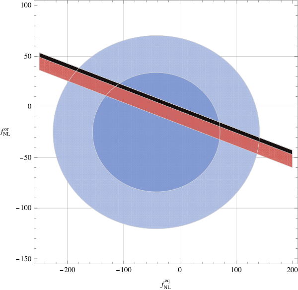
The main result we wish to report in this note is that not only a detectable is possible in this “next-to-minimal” scenario, but its shape is very tightly constrained (Fig. 2). This means – assuming that the tensor/scalar ratio is in fact large – that a detection of non-Gaussianity with a shape that does not lie in the narrow region plotted in Fig. 2 would have dramatic implications for the theory of inflation and fundamental physics in general.
I Effective Theory of Inflation
The effective theory of inflation is based on the fundamental organizing principle of effective field theory: one should write an action containing all terms compatible with the underlying symmetries, starting from the terms most relevant at low energies. In the case of inflation the symmetries are those of de Sitter spacetime, with time-translation invariance weakly broken by slow-roll corrections. The appropriate metric to describe background plus fluctuations can be written in ADM form:
| (1) |
where the background is quasi de Sitter: , , , with a slowly varying function of . The effective action for perturbations of single field inflation, in unitary gauge and to cubic order in perturbations, is
| (2) |
Here , where is the extrinsic curvature , and the are constants with dimensions of mass. The refers to terms of higher order in derivatives or fluctuations.
The first line in (2) incorporates all single-field models with canonical kinetic terms. As mentioned above, these models produce negligible non-Gaussianity. The terms in the second line arise from non-canonical kinetic terms, and can produce large . The main result of this paper is that the Planck and BICEP2 data constrain these terms in such a way that the shape of non-Gaussianity they produce is very sharply defined (Fig. 2). The terms in the third line come from higher derivative terms that cannot be removed by integration by parts, as in ghost condensation [11], or perhaps from Lorentz-breaking modifications of gravity. These terms can produce non-Gaussianity with various different shapes, and – because they indicate exotic physics – experimental confirmation that they are important for the dynamics of inflation would be of great importance.
We introduce the Goldstone boson of broken time translations by making the diffeomorphism:
| (3) |
As we are interested in non-negligible non-Gaussianities (), we can neglect metric perturbations.
| (4) |
where again indicate terms of higher order in derivatives or fluctuations.
In general, for a scalar field in de Sitter space with Lagrangian
| (5) |
the speed of propagation is and we get the power spectrum
| (6) |
where the dimensionless power spectrum is defined by .
Let us pause to briefly discuss tensors. The tensor perturbations are defined by setting
| (7) |
with , . The kinetic term for comes from the Einstein-Hilbert term in (2), with a correction from the term:
| (8) |
This shows there is a modification of the tensor speed of sound, . This differs significantly from only if is close to the Planck mass. Even in this case the resulting tensor non-Gaussianity will be only enhanced compared to its ordinary (undetectably small) value. For this reason we ignore tensors as a source for non-Gaussianity. The tensor power spectrum is given by
| (9) |
II “Next-to-minimal” models of inflation
The class of models with arise from theories with a non-canonical kinetic term for a scalar field , where is a function and . With , eq. (4) simplifies to
| (10) |
where we defined and , so that stays well defined in the limit . For reference, the parameter is defined by . The tensor-to-scalar ratio in this model is
| (11) |
Since and Planck measured [5], one concludes that cannot deviate substantially from :
| (12) |
The non-Gaussianity induced by the operator is proportional to , and therefore cannot be very large if is large. However, the term can still give a sizable contribution to the non-Gaussianity if .
Quantum loops in the effective theory generate [12, 13]. Hence, absent fine-tuning, generates . One might expect the converse to hold as well: that generates small . However this is not the case. Up to cubic order there is no diagram that generates from . Therefore, with is technically natural 11 1 Expanding (4) to quartic order in fluctuations gives a term , which together with generates , but this is suppressed both by a loop factor and the fact that it arises from a quartic term. Another way of seeing the same thing is to compute the 1-loop wave-function renormalization of due to the interaction . This gives rise at most to . [4].
In Fig. 1 we plot the shape of the bispectrum induced by the operator, as a function of the two independent ratios of the triangle sides. Notice that this shape has a large flattened limit (triangles with ).

In Fig. 2 we plot the possible values of in the equilateral/orthogonal plane [15] in (10), with the Planck constraints superimposed [5]. As is evident, (and therefore a large speed of sound) puts a very sharp constraint on the possible shape of non-Gaussianity in this class of models. In the “next-to-minimal” models the region above the line in Fig. 2 can be reached only allowing negative , and as such it would signal exotic physics even if is small.
Dirac-Born-Infeld inflation:
The case of DBI inflation [16] is . The non-Gaussianity is if , from the measurement of tensor modes.
III Other possibilities
If a future experiment detects primordial non-Gaussianity with a shape that does not fall in the narrow region indicated in Fig. 2, what are the implications? In this section we enumerate the set of models consistent with such an observation. All of them differ sharply from the simple model considered above, and correspond to novel physics.
III.1 Quasi-de Sitter
If the background evolution is such that , the standard gradient kinetic term for the perturbations vanishes. In this case, the additional terms in the effective action become important. To simplify the analysis, we consider two limiting cases, depending on whether or dominates, where , and . All the models in this class could potentially be tested by their prediction of near-exact scale invariance for tensor perturbations.
:
This case corresponds to a standard two-derivative kinetic term. The Lagrangian is
| (13) |
The last term seems to imply an additional shape of non-Gaussianity. However, using the linear equations of motion and integrating by parts, it can be rewritten in terms of the standard one-derivative cubic terms:
| (14) |
where the sound speed now is . The interesting fact is that the tensor-to-scalar ratio now does not put strong constraints on the speed of sound:
| (15) |
The requirement that the cutoff has to be gives the constraint . The resulting non-Gaussianity falls in the upper right corner of the plane, above the line in Fig. 2.
:
This case corresponds to the ghost inflation regime [17]. The Lagrangian has a non-relativistic scaling for the kinetic term, which results in non-standard scaling dimensions for energy, momentum, and fields. The most relevant operators are:
| (16) |
The cubic operators proportional to , are suppressed by . In this situation, the tensor-to-scalar ratio is
| (17) |
Again, does not impose strong constraints on the non-Gaussianity, which is very close to the equilateral template.
Notice that in the original work on ghost inflation [17], tensor modes are taken to be negligible because of constraints on the scale from solar system tests of gravity. However, in the effective theory approach, it is perfectly possible that the Lagrangian describing the inflationary perturbations is different from the one describing modifications of gravity today, so this constraint may not play a role. For a recent discussion, see [18].
III.2 Negative speed of sound
It is possible to have consistent models in which , which violate the null energy conditions and give a blue tensor tilt. The speed of sound squared will be negative, which naively implies an instability of the theory. However, the higher derivative gradient kinetic term will make the theory stable at short length scales, which renders these models viable. Depending on the relative size of the two gradient terms, the non-Gaussianity can be very small or extremely large (and already ruled out), but current constraints on do not put a stronger bound.
III.3 Higher-derivative operators
It is possible to impose a “Galilean” symmetry on the effective theory of perturbations which suppresses the single-derivative cubic interactions [19]. In this case, one has a standard kinetic term (with unit speed of sound), and a standard tensor-to-scalar ratio . However, there can be sizable non-Gaussianity induced by 5-derivative cubic terms. The shape of the resulting 3-point function is peculiar, being enhanced in the flattened configurations and somewhat suppressed in the equilateral one (see [19] for details). Also, because of the different scaling of the relevant operators, the size of the 4-point function scales as instead of the usual .
III.4 Modified tensor spectrum
As mentioned above, if it is possible to have . Generically this makes the term in (4) very important, which strongly affects the scalar spectrum. However if is tuned to be small or zero, the effect on scalars is small. In this case since , if the tensor/scalar ratio can be large even with [20], removing the constraint that allowed us to make a sharp prediction for the shape of non-Gaussianity.
III.5 Beyond single-field
Models with multiple fields are much less well constrained. For instance, a model in which a small fraction of the perturbations are generated by a curvaton can evade isocurvature constraints, but if the fluctuations of the curvaton are highly non-Gaussian this could produce relatively large . Another class of examples are dissipative models such as [21, 22, 23], which produces flattened non-Gaussianity. Yet another possibility is quasi-single field inflation [24], whose characteristic is a non-trivial squeezed limit, intermediate between the local and equilateral forms.
IV Conclusions
While the very simplest models of inflation predict undetectably small non-Gaussianity, our analysis shows that the “next-to-minimal” models can produce detectable , but with a shape that is very tightly constrained by BICEP2’s measurement of . Therefore, a measurement of non-Gaussianity with a shape that is inconsistent with this constraint indicates the presence of important new physics: either multiple light fields that strongly affect the inflationary dynamics, or some novel type of higher derivative coupling or violation of Lorentz invariance.
Acknowledgements.
It is a pleasure to thank Paolo Creminelli, Andrei Gruzinov, Nemanja Kaloper, Diana Lpez Nacir, Enrico Pajer, Marko Simonović, Grabriele Trevisan, Filippo Vernizzi, and Matias Zaldarriaga for useful discussions. The work of G. D’A. is supported by NASA through grant NNX10A171G and by NSF through AST-1109432. The work of MK is supported in part by the NSF through grant PHY-1214302 and by the John Templeton Foundation. The opinions expressed in this publication are those of the authors and do not necessarily reflect the views of the John Templeton Foundation.References
- [1] A. D. Linde, Phys.Lett. B129, 177 (1983).
- [2] N. Kaloper and L. Sorbo, Phys.Rev.Lett. 102, 121301 (2009), arXiv:0811.1989 [hep-th] .
- [3] N. Kaloper, A. Lawrence, and L. Sorbo, JCAP 1103, 023 (2011), arXiv:1101.0026 [hep-th] .
- [4] P. Creminelli, D. López Nacir, M. Simonovi?, G. Trevisan, and M. Zaldarriaga, Phys.Rev.Lett. 112, 241303 (2014), arXiv:1404.1065 [astro-ph.CO] .
- [5] P. Ade et al. (Planck Collaboration), (2013a), arXiv:1303.5076 [astro-ph.CO] .
- [6] P. Ade et al. (BICEP2 Collaboration), (2014), arXiv:1403.3985 [astro-ph.CO] .
- [7] J. M. Maldacena, JHEP 0305, 013 (2003), arXiv:astro-ph/0210603 [astro-ph] .
- [8] P. Ade et al. (Planck Collaboration), (2013b), arXiv:1303.5084 [astro-ph.CO] .
- [9] A. Gruzinov, Phys.Rev. D71, 027301 (2005), arXiv:astro-ph/0406129 [astro-ph] .
- [10] C. Cheung, P. Creminelli, A. L. Fitzpatrick, J. Kaplan, and L. Senatore, JHEP 0803, 014 (2008), arXiv:0709.0293 [hep-th] .
- [11] N. Arkani-Hamed, H.-C. Cheng, M. A. Luty, and S. Mukohyama, JHEP 0405, 074 (2004a), arXiv:hep-th/0312099 [hep-th] .
- [12] L. Senatore and M. Zaldarriaga, JCAP 1101, 003 (2011), arXiv:1004.1201 [hep-th] .
- [13] D. Baumann and D. Green, Phys.Rev. D85, 103520 (2012), arXiv:1109.0292 [hep-th] .
- [14] Expanding (4) to quartic order in fluctuations gives a term , which together with generates , but this is suppressed both by a loop factor and the fact that it arises from a quartic term. Another way of seeing the same thing is to compute the 1-loop wave-function renormalization of due to the interaction . This gives rise at most to .
- [15] L. Senatore, K. M. Smith, and M. Zaldarriaga, JCAP 1001, 028 (2010), arXiv:0905.3746 [astro-ph.CO] .
- [16] M. Alishahiha, E. Silverstein, and D. Tong, Phys.Rev. D70, 123505 (2004), arXiv:hep-th/0404084 [hep-th] .
- [17] N. Arkani-Hamed, P. Creminelli, S. Mukohyama, and M. Zaldarriaga, JCAP 0404, 001 (2004b), arXiv:hep-th/0312100 [hep-th] .
- [18] M. M. Ivanov and S. Sibiryakov, JCAP 1405, 045 (2014), arXiv:1402.4964 [astro-ph.CO] .
- [19] P. Creminelli, G. D’Amico, M. Musso, J. Norena, and E. Trincherini, JCAP 1102, 006 (2011), arXiv:1011.3004 [hep-th] .
- [20] T. Noumi and M. Yamaguchi, (2014), arXiv:1403.6065 [hep-th] .
- [21] D. Green, B. Horn, L. Senatore, and E. Silverstein, Phys.Rev. D80, 063533 (2009), arXiv:0902.1006 [hep-th] .
- [22] D. Lopez Nacir, R. A. Porto, L. Senatore, and M. Zaldarriaga, JHEP 1201, 075 (2012), arXiv:1109.4192 [hep-th] .
- [23] G. D’Amico, R. Gobbetti, M. Kleban, and M. Schillo, JCAP 1311, 013 (2013), arXiv:1306.6872 [astro-ph.CO] .
- [24] X. Chen and Y. Wang, JCAP 1004, 027 (2010), arXiv:0911.3380 [hep-th] .