Extreme CII emission in type 2 quasars at z2.5: a signature of -distributed electron energies?
Abstract
We investigate the flux ratio between the 1335 Å and 2326 Å lines of singly ionized carbon in the extended narrow line regions of type 2 quasars at z2.5. We find the observed CII 1335 / CII] 2326 flux ratio, which is not sensitive to the C/H abundance ratio, to be often several times higher than predicted by the canonical AGN photoionization models that use solar metallicity and a Maxwell-Boltzmann electron energy distribution. We study several potential solutions for this discrepancy: low gas metallicity, shock ionization, continuum fluorescence, and -distributed electron energies. Although we cannot definitively distinguish between several of the proposed solutions, we argue that a distribution gives the more natural explanation. We also provide a grid of AGN photoionization models using -distributed electron energies.
Keywords:
quasars: emission lines – galaxies: high-redshift – galaxies: ISM – galaxies: nuclei – galaxies: active1 Introduction
One of the many advantages of looking to the high-redshift Universe is the red-shifting of the rest-frame ultraviolet (UV) emission into the optical observational regime, allowing us to access the unique physics that can be probed using the UV emission or absorption lines.
In this paper we examine the ultraviolet CII 1335 / CII] 2326 flux ratio as a diagnostic of the excitation of extended narrow-line emitting gas associated with active galactic nuclei. Our interest in this flux ratio was initially motivated by the need for indicators of electron temperature (Te) in the rest-frame UV spectral region, to be used with high-z galaxies for which the rest-frame optical temperature diagnostics (i.e., [OIII] 4363 / [OIII] 5007) have been red-shifted out of the optical observational regime. The large difference in excitation energies of the two CII lines (9.3 vs 5.3 eV) makes their flux ratio strongly sensitive to Te, and hence the flux ratio potentially offers a means to determine Te. Furthermore, the use of lines from a singly-ionized species ought to make this diagnostic readily accessible for both high- and low-excitation objects, AGN and star-forming objects, alike (cf. the [NeIV], [NeV] and OIII] high-ionization temperature diagnostics discussed by Humphrey et al. 2008: H08 hereinafter).
In 2 we discuss the observational data used in this paper: the CII 1335 / CII] 2326 flux ratio in type 2, radio-loud quasars at z2.5. These data are compared against different excitation models in 3, and in 4 we discuss the case of the narrow line region of the nearby Seyfert 2 galaxy NGC 1068, which has been extensively observed at UV wavelengths. In 5 we summarize and discuss our findings, and in appendix A1, we give a subset of the exploratory grid of models, using -distributed electron energies, that were computed during the preparation of this paper; the full grid has been made available online.
2 Data from the literature
For this investigation we use line fluxes from the spectropolarimetric study of 9 radio-loud type 2 quasars (also known as radio galaxies), at z2.5 published by Vernet et al. (2001: V01). Of those 9 galaxies, V01 detected 5 of them in both CII 1335 and CII] 2326. The fluxes and line ratios of these two lines are listed in Table 1. Where both lines have been measured, the CII 1335 / CII] 2326 flux ratio occupies the range 0.180.02 - 0.480.07.
3 Comparison against models
3.1 Canonical AGN photoionization models
As has been shown in several previous studies, the UV-optical emission line ratios measured from the narrow line emitting nebulae associated with high redshift type 2 quasars can, in general, be well reproduced using photoionization models that use roughly solar gas metallicity11 1 For solar chemical abundances, we adopt the recent determination by Asplund et al. (2006). , and an ionizing spectrum defined by a power-law of (e.g., Villar-Martín et al. 1997, V01, H08). These models traditionally assume a Maxwell-Boltzmann equilibrium distribution (MBED hereinafter) of electron energies in the ionized plasma.
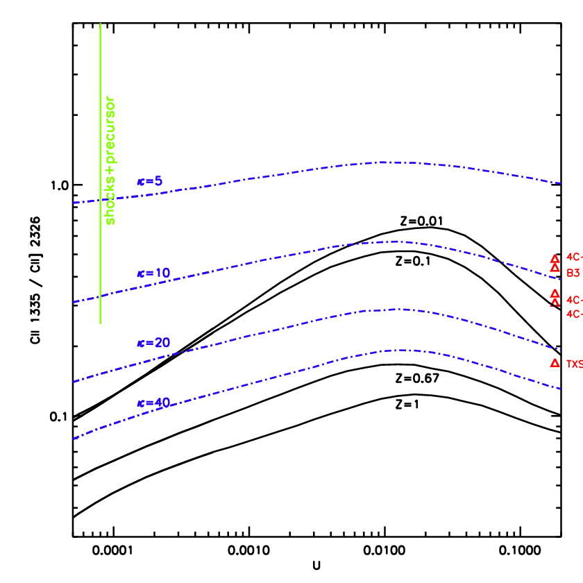
As a starting point, we compute a sequence of models with the above parameters using the photoionization code Mappings 1e (Binette, Dopita & Tuohy 1985; Ferruit et al. 1997; Binette et al. 2012). We adopted a plane-parallel, single-slab geometry with a constant hydrogen density of 100 cm-3. Each model computation was terminated when the hydrogen ionization fraction fell below 1 per cent of its maximum. The ionization parameter U was varied along the model sequence from 110-5 to 0.20. In this solar-metallicity model sequence, the maximum value for the CII 1335 / CII] 2326 flux is 0.11, occurring at U0.01 (Fig. 1). This is a factor of 3 lower than the observed mean value (Table 1), showing that the canonical AGN photoionization models for the extended narrow line emitting gas fail to adequately reproduce the observed CII 1335 / CII] 2326 ratios.
We note that the models also under predict the ratio of CII 1335 relative to several other lines, including Ly, by a similar factor. Furthermore, the low ionization resonant lines SiII 1265 and SiII 1309 are similarly under predicted relative to CII] 2326 and Ly. However, these particular line ratios are additionally subject to relative chemical abundance effects, and hence do not provide as strong a diagnostic power as the CII 1335 / CII] 2326 ratio. For this reason, for the remainder of this paper we will focus on the CII ratio.
While the CII ratio is also sensitive to reddening by dust, any de-reddening would result in an even larger discrepancy between the model and observed CII 1335 / CII] 2326 ratios. We also point out that the CII 1335 / CII] 2326 flux ratio is essentially insensitive to the C/H abundance ratio.
3.2 Sub-solar gas metallicity
Next, we investigate whether sub-solar metallicity ( hereinafter) in the photoionized gas can help to explain the CII 1335 / CII] 2326 ratios. We have repeated the above photoionization calculations, to obtain model sequences at of 0.5, 0.25 and 0.1. All metals were scaled linearly from solar abundances except for nitrogen, which we scaled quadratically (N/O O/H; see e.g. Henry, Edmunds & Köppen 2000; Vernet et al. 2001) from its solar abundance down to =0.25, below which we scaled linearly (N/H O/H). We find that decreasing the gas metallicity yields higher CII 1335 / CII] 2326 ratios, due to the increase in electron temperature as cooling via emission lines becomes less efficient at lower . Consequently, using sub-solar metallicity allows the observed flux ratios to be reproduced (Fig. 1).
While the degeneracy between and U makes it difficult to obtain a precise value of for each object, we can nonetheless use the maximum value of CII 1335 / CII] 2326 at a given to obtain an upper limit on metallicity . The observed values of the line ratio require 0.25, the exception being TXS 0828+193, for which we estimate 0.8. Taken at face value, such low gas metallicities are at odds with the values 1 for several of these type 2 quasars, as estimated in previous studies using the nitrogen lines such as NV 1240 or [NII] 6583 (see V01 and H08).
| Galaxy | z | CII 1335 | CII] 2326 | 1335 / 2326 |
| B3 0731+438 | 2.43 | 2.20.2 | 5.00.5 | 0.440.06 |
| TXS 0828+193 | 2.57 | 3.30.3 | 19.21.9 | 0.170.02 |
| 4C-00.54 | 2.36 | 1.10.1 | 3.60.4 | 0.310.04 |
| 4C+40.36 | 2.27 | 20.92.1 | 43.34.3 | 0.480.07 |
| 4C+48.48 | 2.34 | 3.90.4 | 11.61.2 | 0.340.05 |
| mean | 0.35 | |||
| median | 0.34 |
3.3 -distributed electron energies
Recently, Nicholls et al. (2012, 2013) explored the possibility that electrons in Hii regions and PNe depart from a standard Maxwell-Boltzmann equilibrium energy distribution. To represent non-Maxwell-Boltzmann electron energy distributions, these authors adopted the parametrization given by a –distribution, which is a generalized Lorentzian distribution initially introduced by Vasyliunas (1968). It is widely used in the studies of solar system plasmas (Livadiotis & McComas 2011; Livadiotis et al. 2011) where evidence of suprathermal electron energies abounds. Nicholls et al. found that –distributed electron energies resolved many of the difficulties encountered when attempting to reproduce the temperatures observed in nebulae.
The –distribution is a function of temperature and . When compared to the standard MBED, it results in an excess of electrons (or suprathermal tail) at high energies. The smaller , the larger the excess becomes. This has the effect of substantially enhancing the excitation rates of lines with a high excitation energy as well as reducing the recombination rates (see detailed study of Nicholls et al. 2013). In the limit as , the distribution becomes a MBED. Note that the electron mean energy is the same for a distribution as for a MBED (). Binette et al. (2012) found that a –distribution better reproduces the excess in [O iii] temperatures over that of the [S iii] temperatures, which is found in Hii galaxies, giant extragalactic Hii regions, Galactic Hii regions, and Hii regions from the Magellanic Clouds. Nicholls et al. proposed various mechanisms that would result in a suprathermal distribution, such as (1) magnetic reconnection followed by the migration of high-energy electrons along field lines, and by the development of inertial Alfvén waves, (2) the ejection of high-energy electrons from the photoionization process itself (when the ultraviolet source is very hard, as in PNe or AGN), (3) or from photoionization of dust (Dopita & Sutherland 2000), and (4) by X-ray ionization, resulting in highly energetic (keV) inner-shell (Auger process) electrons (e.g., Aldrovandi & Gruenwald 1985).
Mappings 1e allows the usage of a distribution of electron energies in place of the standard Maxwell-Boltzmann distribution (see Binette et al. 2012). We have computed a grid of models using identical parameters to those used for our canonical model grid described in 3.1, but with -distributed electron energy distributions corresponding to = 2.5, 5, 10, 20, 40, 80.
As described by Nicholls et al. (2012, 2013) and Binette et al. (2012), one of the effects of using a distribution is the general relative enhancement of collisionally excited lines with higher excitation energies. As shown in Fig. 1, this is indeed the case for the CII 1335 / CII] 2326 flux ratio. In order to reproduce the observed flux ratios, we require 1040. This is broadly consistent with the range 1020 deduced by Nicholls et al. (2012) for stellar-photoionized HII regions and planetary nebulae.
A subset of our distribution model grid is shown in Appendix A1, with the complete grid made available online.
3.4 Shock models
In addition to photoionization by the radiation field of the active nucleus, fast shocks driven by the radio jets have also been proposed to contribute to the ionization of the extended narrow line emitting gas in radio-loud active galaxies of the kind considered herein (e.g. Sutherland et al. 1993; Best, Longair & Röttgering 2000; De Breuck et al. 2000; Bicknell et al. 2000; Inksip et al. 2002; H08).
In Fig. 1 we also show the range of the CII 1335 / CII] 2326 ratio produced by the shock models of Allen et al. (2008), for shocks velocities ranging from 100 to 1000 km s-1, with =3.23 G cm3/2 and solar chemical abundances. For the line ratio under consideration, the models show no significant difference between the shock only and shock with precursor models, and thus we show only the latter. In the interest of clarity, the shock models have been plotted at an arbitrary value of U.
From Fig. 1 we can see that the shock models predict significantly higher values for the CII 1335 / CII] 2326 flux ratio than are predicted by our canonical photoionization models. With the exception of TXS 0828+193, the shock models are able to reproduce the measured CII ratios.
3.5 Continuum Fluorescence through CII 1335
The CII 1335 / CII] 2326 flux ratio can also be affected by resonance scattering. This is because the observed flux of a resonant line (i.e. CII 1335 ) can be diminished or enhanced relative to non-resonant lines (i.e., CII] 2326), depending on the gaseous geometry of a system (e.g. Villar-Martín, Binette & Fosbury 1996).
Indeed, recent detections of linearly polarized Ly emission from large-scale gaseous nebulae at high redshift have shown that Ly or continuum fluorescence, via illumination of neutral hydrogen by a central source, is partly responsible for some of the Ly emission for at least a fraction of giant Ly nebulae (Hayes, Scarlata & Siana 2011; Humphrey et al. 2013; see also Prescott et al. 2011). This process can also be expected to result in the continuum fluorescence through other resonant lines, provided that the relevant species are present and that the illuminating radiation field contains photons at the wavelength of the relevant line.
To accurately calculate the luminosity of CII 1335 photons arising by continuum fluorescence, detailed knowledge would be needed of the column density and covering factor of singly ionized carbon, in addition to the continuum luminosity of the quasar at 1335 Å, and would also require careful consideration of the radiative transfer of the CII 1335 through the gaseous environment of the galaxies. Nevertheless, we can provide a ball-park estimate using some simplifying assumptions.
We consider a partially obscured, luminous quasar, which illuminates gas in its host galaxy via a pair of diametrically opposed ionization cones with a total opening angle of 2 Sr. Assuming the hidden quasar is near the top of the luminosity function, we adopt a specific luminosity of 51043 erg s-1 Å-1 near the wavelength of CII 1335, which corresponds to a flux density of 310-16 erg s-1 cm-2 Å-1 at z2. We adopt a gaseous geometry such that one third of sight-lines to the quasar have a radially integrated column density of singly ionized carbon of 1014 cm-2, with no gas along all other sight lines.
Evaluating the total flux of the continuum photons that scattered through the CII 1335 line, we then obtain 10-17 erg s-1 cm-2 – the same order of magnitude as the observed CII 1335 fluxes in the type 2 quasars (Table 1). Clearly, our estimate is subject to large uncertainties, but this exercise does show that continuum fluorescence via AGN continuum illumination is able to make a potentially significant enhancement to the luminosity of the CII 1335 lines in the host galaxies of powerful AGN.
In addition to CII 1335 (and Ly), this effect could potentially enhance other resonant lines. Lines from astrophysically abundant elements, which have a low collisional excitation probability together with a high oscillator strength (e.g. OI 1302, CI 1277 or CI 1560), are expected to show the highest relative flux enhancements.
4 The NLR of NGC 1068
In addition to luminous active galaxies at high redshifts, relatively nearby Seyfert galaxies offer an alternative window by which the ultraviolet spectrum of extended, narrow line emitting gas may be viewed. Among these, the nearby Seyfert 2 galaxy NGC 1068 is one of the most extensively studied, and its narrow line region has been the subject of several of ultraviolet spectroscopic observations using space-based telescopes, which have revealed a spectrum rich in lines from a wide range of metallic species, as well as recombination lines from HI and HeII (e.g., Snijders et al. 1986; Kriss et al. 1992; Kraemer et al. 1998; Kraemer & Crenshaw 2000, hereinafter KC00).
Although photoionization by the AGN is generally able to reproduce the UV-optical emission line spectrum of the narrow line region of NGC 1068 (see e.g. KC00), several of the UV emission lines are substantially at odds with the predictions of photoionization models that use a MBED of electron energies. Interestingly, KC00 noted that in the NLR of NGC 1068 the observed CII 1335 flux, relative to H (or CII] 2326), is about an order of magnitude higher than predicted by the photoionization models that provide a good fit to the overall UV-optical line spectrum. The presence of this CII problem in NGC 1068 suggests that it may in fact be a general problem for AGN photoionized regions, rather than being a problem associated only with powerful quasars.
By including the effects of resonant scattering of the AGN’s anisotropic continuum emission, KC00 were able to enhance the relative flux of the CII 1335 line to match the observed value. Resonant scattering has also been invoked by Ferguson et al. (1995) in order to explain the larger than expected CIII 977 / CIII] 1909 and NIII 990 / NIII] 1749 flux ratios measured by Kriss et al. (1992) in the NLR of NGC 1068.
As discussed in 3.3, our photoionization models using -distributed electron energies are able to produce a substantial enhancement in the flux of CII 1335 relative to CII] 2326 and H. Interestingly, these models also predict a strong enhancement in CIII 977 / CIII] 1909 and NIII 990 / NIII] 1749 ratios. Thus, as a potential new alternative to shock excitation (Kriss et al. 1992) or resonant scattering (Ferguson et al. 1995; KC00), we propose -distributed electron energies as the reason for the discrepancy between observations and photoionization models for these CII, CIII and NIII lines. Detailed modeling of the narrow line region of NGC 1068 using a distribution is beyond the scope of this paper, but will be presented in a future work.
5 Discussion
While investigating the CII 1335 / CII] 2326 emission line ratio as a potential diagnostic of the temperature, metallicity and excitation in ionized nebulae at high redshift, we have identified a failure of canonical photoionization models of the narrow-line emitting ionized gas associated with several type 2, radio-loud quasars at z2.5: the models substantially under-produce CII 1335 relative to CII] 2326. Given that the narrow line region of NGC 1068 shows a similar CII problem to the quasars (KC00), we suggest that this may be a general problem in fitting the narrow line emitting gases of active galaxies, rather than being an issue specific only to powerful quasars.
We have considered several potential causes to explain the higher than predicted CII 1335 / CII] 2326 ratio in the type 2 quasars: substantially sub-solar gas metallicity; ionization by shocks; continuum fluorescence; or -distributed electron energies. We consider the hypothesis involving -distributed electron energies to be the most promising. It represents what we believe to be the simplest solution to the CII problem, insofar as it does not require the presence of a ionizing sources other than the radiation field of the AGN, nor does it require the summation of multiple models with different input parameters. Moreover, -distributed electron energies have been shown to be successful in solving other, long-standing problems in stellar-photoionized HII regions (see Nicholls et al. 2012, 2013; Binette et al. 2012), and are already widely used in studies of plasmas in the solar system (e.g. Livadiotis & McComas 2011; Livadiotis et al. 2011).
We find continuum fluorescence through CII 1335, which enhances the flux of the line above that produced by simple AGN-photoionization, to be another interesting possibility. Given the presence of singly ionized carbon within the beams of AGN UV continuum radiation fields, it seems quite likely that CII 1335 (and other resonant lines) could undergo some enhancement by this process. However, the strength of this effect depends on several difficult to constrain properties, such as the three-dimensional geometry of gas in the host galaxy, and the UV continuum luminosity of the hidden quasar nucleus.
The z2.5 type 2 quasars considered in this work are all radio-loud, and are near the top of the radio luminosity function for AGNs (e.g. Miley & De Breuck 2008). There is a growing body of evidence to suggest that at least in some radio-loud active galaxies, shocks may contribute to the ionization of the extended narrow line emitting gas (e.g. Clark et al. 1998; Villar-Martín et al. 1999; Best, Röttgering & Longair 2000; Bicknell et al. 2000; De Breuck et al. 2000; Inskip et al. 2002; H08; Humphrey et al. 2010). As such, it would seem entirely reasonable for shocks to contribute to the ionization of the extended narrow emission line regions of the distant quasars we have considered herein. However, this would need to be additional to a strong contribution from photoionization by the central AGN, in order to explain the flux ratios of the bright optical emission lines such as [OIII] 4959,5007, [NeV] 3426, H, etc (see, e.g., H08).
Low gas metallicity is the least appealing of the hypotheses we have considered. Although the AGN-photoionization models using low gas metallicity are able to match the observed CII 1335 to CII] 2326 flux ratios in the type 2 quasars, which is due to having higher electron temperature, we point out that low metallicities are at odds with the findings of several earlier studies which concluded that the UV-optical emission line spectra of type 2 quasars are best explained by photoionization models with solar or super-solar gas metallicities (e.g., Robinson et al. 1987; V01; H08; Villar-Martín et al. 2008). The presence of pockets of low metallicity gas, within higher metallicity gaseous halos (Tornatore et al. 2007; Cassata et al. 2013) may provide a means to explain the apparently discrepant implied gas metallicities.
Acknowledgments
AH acknowledges a Marie Curie Fellowship co-funded by the 7th Research Framework Programme and the Portuguese Fundação para a Ciência e a Tecnologia. LB acknowledges support from CONACyT grant CB-128556. We thank the anonymous referee for suggestions that improved our manuscript.
References
- Aldrovandi & Gruenwald (1985) Aldrovandi, S. M. V., & Gruenwald, R. D. 1985, A&A, 147, 331
- Allen et al. (2008) Allen M. G., Groves B. A., Dopita M. A., Sutherland R. S., Kewley L. J., 2008, ApJS, 178, 20
- Asplund, Grevesse, & Jacques Sauval (2006) Asplund M., Grevesse N., Jacques Sauval A., 2006, NuPhA, 777, 1
- Best, Röttgering, & Longair (2000) Best P. N., Röttgering H. J. A., Longair M. S., 2000, MNRAS, 311, 23
- Bicknell et al. (2000) Bicknell G. V., Sutherland R. S., van Breugel W. J. M., Dopita M. A., Dey A., Miley G. K., 2000, ApJ, 540, 678
- Binette, Dopita, & Tuohy (1985) Binette L., Dopita M. A., Tuohy I. R., 1985, ApJ, 297, 476
- Binette et al. (2012) Binette L., Matadamas R., Hägele G. F., Nicholls D. C., Magris C. G., Peña-Guerrero M. Á., Morisset C., Rodríguez-González A., 2012, A&A, 547, A29
- Cassata et al. (2013) Cassata P., et al., 2013, A&A, 556, A68
- Clark et al. (1998) Clark N. E., Axon D. J., Tadhunter C. N., Robinson A., O’Brien P., 1998, ApJ, 494, 546
- De Breuck et al. (2000) De Breuck C., Röttgering H., Miley G., van Breugel W., Best P., 2000, A&A, 362, 519
- Dopita & Sutherland (2000) Dopita, M. A., & Sutherland, R. S. 2000, ApJ, 539, 742
- Ferguson, Ferland, & Pradhan (1995) Ferguson J. W., Ferland G. J., Pradhan A. K., 1995, ApJ, 438, L55
- Ferruit et al. (1997) Ferruit P., Binette L., Sutherland R. S., Pecontal E., 1997, A&A, 322, 73
- Hayes, Scarlata, & Siana (2011) Hayes M., Scarlata C., Siana B., 2011, Natur, 476, 304
- Humphrey et al. (2008) Humphrey A., Villar-Martín M., Vernet J., Fosbury R., di Serego Alighieri S., Binette L., 2008, MNRAS, 383, 11
- Humphrey et al. (2010) Humphrey A., Villar-Martín M., Sánchez S. F., Martínez-Sansigre A., Delgado R. G., Pérez E., Tadhunter C., Pérez-Torres M. A., 2010, MNRAS, 408, L1
- Humphrey et al. (2013) Humphrey A., Vernet J., Villar-Martín M., di Serego Alighieri S., Fosbury R. A. E., Cimatti A., 2013, ApJ, 768, L3
- Inskip et al. (2002) Inskip K. J., Best P. N., Rawlings S., Longair M. S., Cotter G., Röttgering H. J. A., Eales S., 2002, MNRAS, 337, 1381
- Kraemer, Ruiz, & Crenshaw (1998) Kraemer S. B., Ruiz J. R., Crenshaw D. M., 1998, ApJ, 508, 232
- Kraemer & Crenshaw (2000) Kraemer S. B., Crenshaw D. M., 2000, ApJ, 532, 256
- Kriss et al. (1992) Kriss G. A., Davidsen A. F., Blair W. P., Ferguson H. C., Long K. S., 1992, ApJ, 394, L37
- Livadiotis & McComas (2011) Livadiotis, G. & McComas, D. J. 2011, ApJ, 741, 88
- Livadiotis et al. (2011) Livadiotis, G., McComas, D. J., Dayeh, M. A., et al. 2011, ApJ, 734, 1
- Miley & De Breuck (2008) Miley G., De Breuck C., 2008, A&ARv, 15, 67
- Nicholls, Dopita, & Sutherland (2012) Nicholls D. C., Dopita M. A., Sutherland R. S., 2012, ApJ, 752, 148
- Nicholls et al. (2013) Nicholls D. C., Dopita M. A., Sutherland R. S., Kewley L. J., Palay E., 2013, ApJS, 207, 21
- Prescott et al. (2011) Prescott M. K. M., Smith P. S., Schmidt G. D., Dey A., 2011, ApJ, 730, L25
- Robinson et al. (1987) Robinson A., Binette L., Fosbury R. A. E., Tadhunter C. N., 1987, MNRAS, 227, 97
- Snijders, Netzer, & Boksenberg (1986) Snijders M. A. J., Netzer H., Boksenberg A., 1986, MNRAS, 222, 549
- Sutherland, Bicknell, & Dopita (1993) Sutherland R. S., Bicknell G. V., Dopita M. A., 1993, ApJ, 414, 5
- Tornatore, Ferrara, & Schneider (2007) Tornatore L., Ferrara A., Schneider R., 2007, MNRAS, 382, 945
- Vasyliunas (1968) Vasyliunas, V. M. 1968, ASSL, 73, 2839x
- Vernet et al. (2001) Vernet J., Fosbury R. A. E., Villar-Martín M., Cohen M. H., Cimatti A., di Serego Alighieri S., Goodrich R. W., 2001, A&A, 366, 7
- Villar-Martin, Binette, & Fosbury (1996) Villar-Martin M., Binette L., Fosbury R. A. E., 1996, A&A, 312, 751
- Villar-Martin, Tadhunter, & Clark (1997) Villar-Martin M., Tadhunter C., Clark N., 1997, A&A, 323, 21
- Villar-Martín et al. (1999) Villar-Martín M., Tadhunter C., Morganti R., Axon D., Koekemoer A., 1999, MNRAS, 307, 24
- Villar-Martín et al. (2008) Villar-Martín M., Humphrey A., Martínez-Sansigre A., Pérez-Torres M., Binette L., Zhang X. G., 2008, MNRAS, 390, 218
Appendix A1: AGN photoionization model grid using a -distribution
Here we describe the grid of photoionization models with -distributed electron energies that were computed during the preparation of this paper. All models adopt a plane parallel, single-slab geometry with a constant hydrogen density of 100 cm-3, illuminated by an ionizing continuum of spectral shape with a high-energy cut-off of 5104 eV. Computation was terminated once the hydrogen ionization fraction fell to 1 per cent of its maximum. Input parameters were varied as follows; was set to 2.5, 5, 10, 20, 40, or 80; ionization parameter U was varied from 0.00001 to 0.20 in steps of factor 3; the gas metallicity was set to solar, half solar, or twice solar, with all metal abundances scaled linearly with O/H, except for N/H which we scaled from its solar value as N/O O/H to represent secondary nitrogen enrichment. For a subset of our model grid we show fluxes of various emission lines, normalized to H, in Table A1. For completeness, in Table A2 we also show output from models with identical input parameters except for , which we set to to simulate a Maxwell-Boltzmann distribution of electron energies. The full grid of models described in this appendix is available online.
| 40 | 40 | 40 | 40 | 20 | 20 | 20 | 20 | 10 | 10 | 10 | 10 | |
|---|---|---|---|---|---|---|---|---|---|---|---|---|
| Log U | -3.6 | -2.6 | -1.7 | -0.7 | -3.6 | -2.6 | -1.7 | -0.7 | -3.6 | -2.6 | -1.7 | -0.7 |
| C III 977 | 3.51e-03 | 4.19e-02 | 3.74e-01 | 2.19e-01 | 1.13e-02 | 1.18e-01 | 6.28e-01 | 3.00e-01 | 1.59e-02 | 4.20e-01 | 1.42e+00 | 5.73e-01 |
| N III 990 | 4.39e-05 | 1.77e-03 | 1.49e-02 | 8.77e-03 | 1.61e-04 | 5.00e-03 | 2.50e-02 | 1.12e-02 | 7.00e-05 | 1.78e-02 | 5.66e-02 | 1.84e-02 |
| O VI 1036 | 1.61e-09 | 5.31e-05 | 2.18e-01 | 7.85e+00 | 5.37e-09 | 1.23e-04 | 2.97e-01 | 8.71e+00 | 3.92e-11 | 3.47e-04 | 4.65e-01 | 1.02e+01 |
| C II 1037 | 2.09e-03 | 2.50e-03 | 1.61e-03 | 3.94e-04 | 4.95e-03 | 5.41e-03 | 2.69e-03 | 6.25e-04 | 1.44e-02 | 1.48e-02 | 5.67e-03 | 1.15e-03 |
| Si III 1207 | 1.40e-03 | 8.81e-03 | 4.44e-03 | 8.31e-04 | 3.00e-03 | 1.72e-02 | 6.35e-03 | 1.05e-03 | 1.02e-04 | 3.86e-02 | 1.04e-02 | 1.41e-03 |
| H I 1216 | 2.95e+01 | 2.90e+01 | 2.69e+01 | 2.59e+01 | 3.14e+01 | 3.04e+01 | 2.76e+01 | 2.62e+01 | 3.62e+01 | 3.18e+01 | 2.85e+01 | 2.66e+01 |
| N V 1240 | 6.32e-07 | 7.58e-04 | 2.12e-01 | 1.02e+00 | 1.43e-06 | 1.39e-03 | 2.62e-01 | 1.09e+00 | 3.33e-08 | 2.93e-03 | 3.60e-01 | 1.22e+00 |
| Si II 1260 | 2.03e-02 | 1.81e-02 | 8.44e-03 | 2.47e-03 | 3.42e-02 | 2.64e-02 | 1.06e-02 | 3.04e-03 | 4.17e-02 | 4.34e-02 | 1.41e-02 | 3.74e-03 |
| Si II 1309 | 6.78e-03 | 5.89e-03 | 2.70e-03 | 8.03e-04 | 1.08e-02 | 8.15e-03 | 3.25e-03 | 9.43e-04 | 1.14e-02 | 1.25e-02 | 4.05e-03 | 1.09e-03 |
| C II 1335 | 6.52e-02 | 6.16e-02 | 2.92e-02 | 8.69e-03 | 9.75e-02 | 8.85e-02 | 3.63e-02 | 1.01e-02 | 1.10e-01 | 1.44e-01 | 5.00e-02 | 1.16e-02 |
| Si IV 1397 | 1.83e-03 | 1.03e-01 | 1.19e-01 | 3.69e-02 | 3.24e-03 | 1.74e-01 | 1.76e-01 | 5.26e-02 | 1.82e-04 | 3.25e-01 | 3.13e-01 | 9.13e-02 |
| O IV 1400 | 1.37e-05 | 1.01e-02 | 4.29e-01 | 7.55e-01 | 2.59e-05 | 1.59e-02 | 4.99e-01 | 7.75e-01 | 3.70e-07 | 2.76e-02 | 6.23e-01 | 7.77e-01 |
| N IV 1486 | 2.07e-05 | 7.17e-03 | 2.26e-01 | 3.37e-01 | 3.59e-05 | 1.08e-02 | 2.65e-01 | 3.74e-01 | 6.86e-07 | 1.77e-02 | 3.41e-01 | 4.53e-01 |
| C IV 1549 | 4.18e-04 | 9.74e-02 | 3.48e+00 | 4.22e+00 | 6.63e-04 | 1.40e-01 | 4.10e+00 | 5.04e+00 | 2.32e-05 | 2.11e-01 | 5.29e+00 | 7.02e+00 |
| Ne V 1575 | 6.40e-09 | 2.74e-05 | 7.79e-03 | 3.05e-02 | 1.01e-08 | 3.77e-05 | 8.49e-03 | 3.08e-02 | 1.06e-10 | 5.34e-05 | 9.50e-03 | 3.08e-02 |
| Ne IV 1602 | 3.59e-06 | 4.29e-04 | 7.60e-03 | 7.75e-03 | 5.52e-06 | 5.96e-04 | 8.50e-03 | 8.06e-03 | 2.01e-07 | 8.67e-04 | 1.00e-02 | 8.42e-03 |
| He II 1640 | 7.75e-01 | 1.35e+00 | 1.53e+00 | 1.39e+00 | 7.25e-01 | 1.31e+00 | 1.51e+00 | 1.39e+00 | 2.96e-01 | 1.19e+00 | 1.47e+00 | 1.41e+00 |
| O III 1663 | 1.78e-03 | 3.49e-02 | 1.20e-01 | 1.74e-01 | 2.63e-03 | 4.88e-02 | 1.50e-01 | 2.03e-01 | 1.63e-04 | 7.09e-02 | 2.09e-01 | 2.63e-01 |
| N III 1749 | 2.92e-03 | 5.61e-02 | 1.42e-01 | 4.03e-02 | 4.04e-03 | 7.50e-02 | 1.67e-01 | 4.60e-02 | 1.82e-04 | 1.02e-01 | 2.14e-01 | 5.72e-02 |
| Mg VI 1806 | 7.29e-10 | 5.32e-05 | 4.40e-02 | 7.15e-02 | 9.64e-10 | 6.47e-05 | 4.65e-02 | 7.25e-02 | 0.00e+00 | 7.58e-05 | 4.93e-02 | 7.32e-02 |
| Si II 1809 | 6.00e-04 | 4.19e-04 | 1.74e-04 | 5.98e-05 | 6.56e-04 | 4.23e-04 | 1.60e-04 | 5.30e-05 | 2.40e-04 | 4.05e-04 | 1.30e-04 | 3.85e-05 |
| Si III 1890 | 4.24e-02 | 1.53e-01 | 4.69e-02 | 8.27e-03 | 4.90e-02 | 1.84e-01 | 4.80e-02 | 7.71e-03 | 4.66e-04 | 2.31e-01 | 4.98e-02 | 6.64e-03 |
| C III 1909 | 2.49e-01 | 1.31e+00 | 2.82e+00 | 9.53e-01 | 2.88e-01 | 1.60e+00 | 3.20e+00 | 1.11e+00 | 3.57e-02 | 1.94e+00 | 3.84e+00 | 1.44e+00 |
| N II 2139 | 3.87e-02 | 2.74e-02 | 8.23e-03 | 1.67e-03 | 3.93e-02 | 2.70e-02 | 7.32e-03 | 1.35e-03 | 8.22e-03 | 2.43e-02 | 5.73e-03 | 8.81e-04 |
| C II 2326 | 5.85e-01 | 3.91e-01 | 1.54e-01 | 6.62e-02 | 5.30e-01 | 3.54e-01 | 1.30e-01 | 5.20e-02 | 1.29e-01 | 2.83e-01 | 9.11e-02 | 2.96e-02 |
| Si II 2335 | 3.90e-01 | 2.38e-01 | 9.55e-02 | 3.69e-02 | 3.62e-01 | 2.10e-01 | 7.86e-02 | 2.92e-02 | 7.79e-02 | 1.59e-01 | 5.19e-02 | 1.69e-02 |
| Ne IV 2424 | 8.39e-04 | 6.01e-02 | 4.94e-01 | 3.26e-01 | 9.09e-04 | 6.51e-02 | 5.00e-01 | 3.26e-01 | 1.32e-05 | 6.65e-02 | 4.99e-01 | 3.20e-01 |
| O II 2471 | 7.58e-02 | 5.20e-02 | 1.42e-02 | 3.02e-03 | 7.31e-02 | 4.98e-02 | 1.28e-02 | 2.57e-03 | 1.05e-02 | 4.20e-02 | 1.02e-02 | 1.88e-03 |
| Mg V 2784 | 5.18e-07 | 3.20e-03 | 1.21e-01 | 4.42e-02 | 5.15e-07 | 3.24e-03 | 1.21e-01 | 4.55e-02 | 1.28e-09 | 2.94e-03 | 1.17e-01 | 4.71e-02 |
| Mg II 2800 | 1.69e+00 | 1.38e+00 | 8.05e-01 | 3.84e-01 | 1.51e+00 | 1.22e+00 | 6.87e-01 | 3.14e-01 | 4.96e-01 | 8.88e-01 | 4.84e-01 | 1.95e-01 |
| Ne V 3426 | 3.59e-06 | 6.27e-03 | 4.69e-01 | 7.62e-01 | 3.39e-06 | 6.07e-03 | 4.50e-01 | 7.44e-01 | 9.28e-09 | 5.15e-03 | 4.04e-01 | 7.00e-01 |
| O II 3727 | 6.00e+00 | 3.32e+00 | 8.21e-01 | 1.95e-01 | 5.23e+00 | 2.94e+00 | 6.96e-01 | 1.55e-01 | 5.45e-01 | 2.15e+00 | 4.89e-01 | 9.57e-02 |
| Ne III 3869 | 3.89e-01 | 8.75e-01 | 1.14e+00 | 1.08e+00 | 3.41e-01 | 8.27e-01 | 1.13e+00 | 1.09e+00 | 1.92e-02 | 6.78e-01 | 1.05e+00 | 1.10e+00 |
| O III 4363 | 5.19e-03 | 7.52e-02 | 1.85e-01 | 2.12e-01 | 5.73e-03 | 8.41e-02 | 2.02e-01 | 2.30e-01 | 1.47e-04 | 8.87e-02 | 2.25e-01 | 2.61e-01 |
| He II 4686 | 1.29e-01 | 2.02e-01 | 1.94e-01 | 1.57e-01 | 1.27e-01 | 1.98e-01 | 1.93e-01 | 1.59e-01 | 7.26e-02 | 1.90e-01 | 1.90e-01 | 1.62e-01 |
| O III 5007 | 9.92e-01 | 8.76e+00 | 1.40e+01 | 1.33e+01 | 8.82e-01 | 8.23e+00 | 1.35e+01 | 1.32e+01 | 1.39e-02 | 6.66e+00 | 1.23e+01 | 1.27e+01 |
| O I 6300 | 7.84e-01 | 4.89e-01 | 2.67e-01 | 1.51e-01 | 5.45e-01 | 3.35e-01 | 1.84e-01 | 1.05e-01 | 4.03e-02 | 1.29e-01 | 7.08e-02 | 3.90e-02 |
| H I 6563 | 2.92e+00 | 2.92e+00 | 2.91e+00 | 2.90e+00 | 2.95e+00 | 2.95e+00 | 2.92e+00 | 2.90e+00 | 3.11e+00 | 2.99e+00 | 2.95e+00 | 2.91e+00 |
| N II 6584 | 2.38e+00 | 1.06e+00 | 2.77e-01 | 7.57e-02 | 1.99e+00 | 8.98e-01 | 2.23e-01 | 5.61e-02 | 2.38e-01 | 6.01e-01 | 1.36e-01 | 2.73e-02 |
| S II 6724 | 1.96e+00 | 8.11e-01 | 5.45e-01 | 3.73e-01 | 1.59e+00 | 6.53e-01 | 4.26e-01 | 2.98e-01 | 3.60e-01 | 3.63e-01 | 2.23e-01 | 1.52e-01 |
| Log U | -3.6 | -2.6 | -1.7 | -0.7 |
|---|---|---|---|---|
| C III 977 | 5.95e-04 | 9.49e-03 | 2.02e-01 | 1.61e-01 |
| N III 990 | 5.36e-06 | 3.91e-04 | 8.04e-03 | 6.71e-03 |
| O VI 1036 | 2.23e-10 | 1.58e-05 | 1.48e-01 | 6.92e+00 |
| C II 1037 | 6.09e-04 | 8.96e-04 | 8.49e-04 | 2.13e-04 |
| Si III 1207 | 3.98e-04 | 3.40e-03 | 2.76e-03 | 5.82e-04 |
| H I 1216 | 2.74e+01 | 2.76e+01 | 2.61e+01 | 2.55e+01 |
| N V 1240 | 1.70e-07 | 3.24e-04 | 1.64e-01 | 9.41e-01 |
| Si II 1260 | 9.56e-03 | 1.09e-02 | 6.03e-03 | 1.78e-03 |
| Si II 1309 | 3.47e-03 | 3.79e-03 | 2.03e-03 | 6.11e-04 |
| C II 1335 | 3.61e-02 | 3.87e-02 | 2.18e-02 | 6.70e-03 |
| Si IV 1397 | 7.15e-04 | 5.01e-02 | 7.45e-02 | 2.40e-02 |
| O IV 1400 | 4.96e-06 | 5.39e-03 | 3.55e-01 | 7.18e-01 |
| N IV 1486 | 8.61e-06 | 4.07e-03 | 1.86e-01 | 3.04e-01 |
| C IV 1549 | 1.97e-04 | 5.87e-02 | 2.87e+00 | 3.56e+00 |
| Ne V 1575 | 3.02e-09 | 1.74e-05 | 6.94e-03 | 2.99e-02 |
| Ne IV 1602 | 1.78e-06 | 2.72e-04 | 6.61e-03 | 7.41e-03 |
| He II 1640 | 8.03e-01 | 1.38e+00 | 1.54e+00 | 1.39e+00 |
| O III 1663 | 9.39e-04 | 2.17e-02 | 9.22e-02 | 1.48e-01 |
| N III 1749 | 1.67e-03 | 3.71e-02 | 1.16e-01 | 3.46e-02 |
| Mg VI 1806 | 4.36e-10 | 3.95e-05 | 4.08e-02 | 7.04e-02 |
| Si II 1809 | 4.95e-04 | 3.96e-04 | 1.81e-04 | 6.33e-05 |
| Si III 1890 | 2.97e-02 | 1.16e-01 | 4.36e-02 | 8.43e-03 |
| C III 1909 | 1.86e-01 | 9.86e-01 | 2.42e+00 | 7.97e-01 |
| N II 2139 | 3.46e-02 | 2.67e-02 | 9.10e-03 | 1.98e-03 |
| C II 2326 | 5.98e-01 | 4.19e-01 | 1.77e-01 | 7.90e-02 |
| Si II 2335 | 3.89e-01 | 2.60e-01 | 1.11e-01 | 4.40e-02 |
| Ne IV 2424 | 6.81e-04 | 5.25e-02 | 4.81e-01 | 3.26e-01 |
| O II 2471 | 7.15e-02 | 5.20e-02 | 1.56e-02 | 3.48e-03 |
| Mg V 2784 | 4.66e-07 | 3.03e-03 | 1.20e-01 | 4.28e-02 |
| Mg II 2800 | 1.74e+00 | 1.48e+00 | 8.98e-01 | 4.41e-01 |
| Ne V 3426 | 3.47e-06 | 6.23e-03 | 4.84e-01 | 7.84e-01 |
| O II 3727 | 6.42e+00 | 3.63e+00 | 9.50e-01 | 2.39e-01 |
| Ne III 3869 | 4.12e-01 | 8.94e-01 | 1.14e+00 | 1.05e+00 |
| O III 4363 | 4.09e-03 | 6.26e-02 | 1.65e-01 | 1.93e-01 |
| He II 4686 | 1.30e-01 | 2.03e-01 | 1.94e-01 | 1.57e-01 |
| O III 5007 | 1.04e+00 | 9.03e+00 | 1.43e+01 | 1.34e+01 |
| O I 6300 | 1.02e+00 | 6.51e-01 | 3.52e-01 | 2.00e-01 |
| H I 6563 | 2.89e+00 | 2.90e+00 | 2.90e+00 | 2.89e+00 |
| N II 6584 | 2.70e+00 | 1.21e+00 | 3.32e-01 | 9.66e-02 |
| S II 6724 | 2.26e+00 | 9.37e-01 | 6.40e-01 | 4.42e-01 |