Log-Concavity and Strong Log-Concavity:
a review

Adrien Saumard^?? Jon A. Wellner^??

Abstract

We review and formulate results concerning log-concavity and strong-log-concavity in both discrete and continuous settings. We show how preservation of log-concavity and strongly log-concavity on $\mathbb{R}$ under convolution follows from a fundamental monotonicity result of Efron (1969). We provide a new proof of Efron’s theorem using the recent asymmetric Brascamp-Lieb inequality due to Otto and Menz (2013). Along the way we review connections between log-concavity and other areas of mathematics and statistics, including concentration of measure, log-Sobolev inequalities, convex geometry, MCMC algorithms, Laplace approximations, and machine learning.

keywords

[class=AMS] Primary 60E15 , 62E10 ; secondary 62H05

keywords

concave , convex , convolution , inequalities , log-concave , monotone , preservation , strong log-concave

and

Departamento de Estadística, CIMFAV
Universidad de Valparaíso, Chile
??

Department of Statistics, Box 354322
University of Washington
Seattle, WA 98195-4322
??

1 Introduction: log-concavity

Log-concave distributions and various properties related to log-concavity play an increasingly important role in probability, statistics, optimization theory, econometrics and other areas of applied mathematics. In view of these developments, the basic properties and facts concerning log-concavity deserve to be more widely known in both the probability and statistics communities. Our goal in this survey is to review and summarize the basic preservation properties which make the classes of log-concave densities, measures, and functions so important and useful. In particular we review preservation of log-concavity and “strong log-concavity” (to be defined carefully in section 2) under marginalization, convolution, formation of products, and limits in distribution. The corresponding notions for discrete distributions (log-concavity and ultra log-concavity) are also reviewed in section 4.

A second goal is to acquaint our readers with a useful monotonicity theorem for log-concave distributions on $\mathbb{R}$ due to Efron [1965], and to briefly discuss connections with recent progress concerning “asymmetric” Brascamp-Lieb inequalities. Efron’s theorem is reviewed in Section 6.1, and further applications are given in the rest of Section 6.

There have been several reviews of developments connected to log-concavity in the mathematics literature, most notably Das Gupta [1980] and Gardner [2002]. We are not aware of any comprehensive review of log-concavity in the statistics literature, although there have been some review type papers in econometrics, in particular An [1998] and Bagnoli and Bergstrom [2005]. Given the pace of recent advances, it seems that a review from a statistical perspective is warranted.

Several books deal with various aspects of log-concavity: the classic books by Marshall and Olkin [1979] (see also Marshall, Olkin and Arnold [2011]) and Dharmadhikari and Joag-Dev [1988] both cover aspects of log-concavity theory, but from the perspective of majorization in the first case, and a perspective dominated by unimodality in the second case. Neither treats the important notion of strong log-concavity. The recent book by Simon [2011] perhaps comes closest to our current perspective with interesting previously unpublished material from the papers of Brascamp and Lieb in the 1970’s and a proof of the Brascamp and Lieb result to the effect that strong log-concavity is preserved by marginalization. Unfortunately Simon does not connect with recent terminology and other developments in this regard and focuses on convexity theory more broadly. Villani [2003] (chapter 6) gives a nice treatment of the Brunn-Minkowski inequality and related results for log-concave distributions and densities with interesting connections to optimal transportation theory. His chapter 9 also gives a nice treatment of the connections between log-Sobolev inequalities and strong log-concavity, albeit with somewhat different terminology. Ledoux [2001] is, of course, a prime source for material on log-Sobolev inequalities and strong log concavity. The nice book on stochastic programming by Prékopa [1995] has its chapter 4 devoted to log-concavity and $s-$ concavity, but has no treatment of strong log-concavity or inequalities related to log-concavity and strong log-concavity. In this review we will give proofs some key results in the body of the review, while proofs of supporting results are postponed to Section 11 (Appendix B).

2 Log-concavity and strong log-concavity: definitions and basic results

We begin with some basic definitions of log-concave densities and measures on $\mathbb{R}^{d}$ .

Definition 2.1.

(0-d): A density function $p$ with respect to Lebesgue measure $\lambda$ on $(\mathbb{R}^{d},\mathcal{B}^{d})$ is log-concave if $p=e^{-\varphi}$ where $\varphi$ is a convex function from $\mathbb{R}^{d}$ to $(-\infty,\infty]$ . Equivalently, $p$ is log-concave if $p=\exp(\tilde{\varphi})$ where $\tilde{\varphi}=-\varphi$ is a concave function from $\mathbb{R}^{d}$ to $[-\infty,\infty)$ .

We will usually adopt the convention that $p$ is lower semi-continuous and $\varphi=-\log p$ is upper semi-continuous. Thus $\{x\in\mathbb{R}^{d}:\ p(x)>t\}$ is open, while $\{x\in\mathbb{R}^{d}:\ \varphi(x)\leq t\}$ is closed. We will also say that a non-negative and integrable function $f$ from $\mathbb{R}^{d}$ to $[0,\infty)$ is log-concave if $f=e^{-\varphi}$ where $\varphi$ is convex even though $f$ may not be a density; that is $\int_{\mathbb{R}^{d}}fd\lambda\in(0,\infty)$ .

Many common densities are log-concave; in particular all Gaussian densities

\displaystyle p_{\mu,\Sigma}(x)=(2\pi|\Sigma|)^{-d/2}\exp\left(-\frac{1}{2}(x-\mu)^{T}\Sigma^{-1}(x-\mu)\right)

with $\mu\in\mathbb{R}^{d}$ and $\Sigma$ positive definite are log-concave, and

\displaystyle p_{C}(x)=1_{C}(x)/\lambda(C)

is log-concave for any non-empty, open and bounded convex subset $C\subset\mathbb{R}^{d}$ . With $C$ open, $p$ is lower semi-continuous in agreement with our convention noted above; of course taking $C$ closed leads to upper semi-continuity of $p$ .

In the case $d=1$ , log-concave functions and densities are related to several other important classes. The following definition goes back to the work of Pólya and Schoenberg.

Definition 2.2.

Let $p$ be a function on $\mathbb{R}$ (or some subset of $\mathbb{R}$ ), and let $x_{1}<\cdots<x_{k}$ , $y_{1}<\cdots<y_{k}$ . Then $p$ is said to be a Pólya frequency function of order $k$ (or $p\in PF_{k}$ ) if $\mbox{det}(p(x_{i}-y_{j}))\geq 0$ for all such choices of the $x$ ’s and $y$ ’s. If $p$ is $PF_{k}$ for every $k$ , then $p\in PF_{\infty}$ , the class of Pólya frequency functions of order $\infty$ .

A connecting link to Pólya frequency functions and to the notion of monotone likelihood ratios, which is of some importance in statistics, is given by the following proposition:

Proposition 2.3.

(a) The class of log-concave functions on $\mathbb{R}$ coincides with the class of Pólya frequency functions of order $2$ .
(b) A density function $p$ on $\mathbb{R}$ is log-concave if and only if the translation family $\{p(\cdot-\theta):\ \theta\in\mathbb{R}\}$ has monotone likelihood ratio: i.e. for every $\theta_{1}<\theta_{2}$ the ratio $p(x-\theta_{2})/p(x-\theta_{1})$ is a monotone nondecreasing function of $x$ .

Proof.

See Section 11. ∎

Definition 2.4.

(0-m): A probability measure $P$ on $(\mathbb{R}^{d},\mathcal{B}^{d})$ is log-concave if for all non-empty sets $A,B\in\mathcal{B}^{d}$ and for all $0<\theta<1$ we have

\displaystyle P(\theta A+(1-\theta)B)\geq P(A)^{\theta}P(B)^{1-\theta}.

It is well-known that log-concave measures have sub-exponential tails, see Borell [1983] and Section 5.1 below. To accommodate densities having tails heavier than exponential, the classes of $s-$ concave densities and measures are of interest.

Definition 2.5.

(s-d): A density function $p$ with respect to Lebesgue measure $\lambda$ on an convex set $C\subset\mathbb{R}^{d}$ is $s-$ concave if

\displaystyle p(\theta x+(1-\theta)y)\geq M_{s}(p(x),p(y);\theta)

where the generalized mean $M_{s}(u,v;\theta)$ is defined for $u,v\geq 0$ by

\displaystyle M_{s}(u,v;\theta)\equiv\left\{\begin{array}[]{ll}(\theta u^{s}+(1-\theta)v^{s})^{1/s},&s\not=0,\\ u^{\theta}v^{1-\theta},&s=0,\\ \mbox{min}\{u,v\},&s=-\infty,\\ \mbox{max}\{u,v\},&s=+\infty.\end{array}\right.

Definition 2.6.

(s-m): A probability measure $P$ on $(\mathbb{R}^{d},\mathcal{B}^{d})$ is $s-$ concave if for all non-empty sets $A,B$ in $\mathcal{B}^{d}$ and for all $\theta\in(0,1)$ ,

\displaystyle P(\theta A+(1-\theta)B)\geq M_{s}(P(A),P(B);\theta)

where $M_{s}(u,v;\theta)$ is as defined above.

These classes of measures and densities were studied by Prékopa [1973] in the case $s=0$ and for all $s\in\mathbb{R}$ by Brascamp and Lieb [1976], Borell [1975], Borell [1974], and Rinott [1976]. The main results concerning these classes are nicely summarized by Dharmadhikari and Joag-Dev [1988]; see especially sections 2.3-2.8 (pages 46-66) and section 3.3 (pages 84-99). In particular we will review some of the key results for these classes in the next section. For bounds on densities of $s-$ concave distributions on $\mathbb{R}$ see Doss and Wellner [2013]; for probability tail bounds for $s-$ concave measures on $\mathbb{R}^{d}$ , see Bobkov and Ledoux [2009]. For moment bounds and concentration inequalities for $s-$ concave distributions with $s<0$ see Adamczak et al. [2012] and Guédon [2012], section 3.

A key theorem connecting probability measures to densities is as follows:

Theorem 2.7.

Suppose that $P$ is a probability measure on $(\mathbb{R}^{d},\mathcal{B}^{d})$ such that the affine hull of $\mbox{supp}(P)$ has dimension $d$ . Then $P$ is a log-concave measure if and only if it has a log-concave density function $p$ on $\mathbb{R}^{d}$ ; that is $p=e^{\varphi}$ with $\varphi$ concave satisfies

P(A)=\int_{A}pd\lambda\ \ \ \mbox{for}\ \ \ A\in\mathcal{B}^{d}.

For the correspondence between $s-$ concave measures and $t-$ concave densities, see Borell [1975], Brascamp and Lieb [1976] section 3, Rinott [1976], and Dharmadhikari and Joag-Dev [1988].

One of our main goals here is to review and summarize what is known concerning the (smaller) classes of (what we call) strongly log-concave densities. This terminology is not completely standard. Other terms used for the same or essentially the same notion include:

•

Log-concave perturbation of Gaussian; Villani [2003], Caffarelli [2000]. pages 290-291.
•

Gaussian weighted log-concave; Brascamp and Lieb [1976] pages 379, 381.
•

Uniformly convex potential: Bobkov and Ledoux [2000], abstract and page 1034, Gozlan and Léonard [2010], Section 7.
•

Strongly convex potential: Caffarelli [2000].

In the case of real-valued discrete variables the comparable notion is called ultra log-concavity; see e.g. Liggett [1997], Johnson, Kontoyiannis and Madiman [2013], and Johnson [2007]. We will re-visit the notion of ultra log-concavity in Section 4.

Our choice of terminology is motivated in part by the following definition from convexity theory: following Rockafellar and Wets [1998], page 565, we say that a proper convex function $h:\mathbb{R}^{d}\rightarrow\overline{\mathbb{R}}$ is strongly convex if there exists a positive number $c$ such that

h(\theta x+(1-\theta)y)\leq\theta h(x)+(1-\theta)h(y)-\frac{1}{2}c\theta(1-\theta)\|x-y\|^{2}

for all $x,y\in\mathbb{R}^{d}$ and $\theta\in(0,1)$ . It is easily seen that this is equivalent to convexity of $h(x)-(1/2)c\|x\|^{2}$ (see Rockafellar and Wets [1998], Exercise12.59, page 565).

Thus our first definition of strong log-concavity of a density function $p$ on $\mathbb{R}^{d}$ is as follows:

Definition 2.8.

For any $\sigma^{2}>0$ define the class of strongly log-concave densities with variance parameter $\sigma^{2}$ , or $SLC_{1}(\sigma^{2},d)$ to be the collection of density functions $p$ of the form

p(x)=g(x)\phi_{\sigma^{2}I}(x)

for some log-concave function $g$ where, for a positive definite matrix $\Sigma$ and $\mu\in\mathbb{R}^{d}$ , $\phi_{\Sigma}(\cdot-\mu)$ denotes the $N_{d}(\mu,\Sigma)$ density given by

\phi_{\Sigma}(x-\mu)=(2\pi|\Sigma|)^{-d/2}\exp\left(-\frac{1}{2}(x-\mu)^{T}\Sigma^{-1}(x-\mu)\right).

(2.2)

If a random vector $X$ has a density $p$ of this form, then we also say that $X$ is strongly log-concave.

Note that this agrees with the definition of strong convexity given above since,

h(x)\equiv-\log p(x)=-\log g(x)+d\log(\sigma\sqrt{2\pi})+\frac{|x|^{2}}{2\sigma^{2}},

so that

-\log p(x)-\frac{|x|^{2}}{2\sigma^{2}}=-\log g(x)+d\log(\sigma\sqrt{2\pi})

is convex; i.e. $-\log p(x)$ is strongly convex with $c=1/\sigma^{2}$ . Notice however that if $p\in SLC_{1}(\sigma^{2},d)$ then larger values of $\sigma^{2}$ corresp to smaller values of $c=1/\sigma^{2}$ , and hence $p$ becomes less strongly log-concave as $\sigma^{2}$ increases. Thus in our definition of strong log-concavity the coefficient $\sigma^{2}$ measures the “flatness” of the convex potential

It will be useful to relax this definition in two directions: by allowing the Gaussian distribution to have a non-singular covariance matrix $\Sigma$ other than the identity matrix and perhaps a non-zero mean vector $\mu$ . Thus our second definition is as follows.

Definition 2.9.

Let $\Sigma$ be a $d\times d$ positive definite matrix and let $\mu\in\mathbb{R}^{d}$ . We say that a random vector $X$ and its density function $p$ are strongly log-concave and write $p\in SLC_{2}(\mu,\Sigma,d)$ if

p(x)=g(x)\phi_{\Sigma}(x-\mu)\ \ \ \mbox{for}\ \ \ x\in\mathbb{R}^{d}

for some log-concave function $g$ where $\phi_{\Sigma}(\cdot-\mu)$ denotes the $N_{d}(\mu,\Sigma)$ density given by (2.2).

Note that $SLC_{2}(0,\sigma^{2}I,d)=SLC_{1}(\sigma^{2},d)$ as in Definition 2.8. Furthermore, if $p\in SLC_{2}(\mu,\Sigma,d)$ with $\Sigma$ non-singular, then we can write

$\displaystyle p(x)$	$\displaystyle=$	$\displaystyle g(x)\frac{\phi_{\Sigma}(x-\mu)}{\phi_{\Sigma}(x)}\cdot\frac{\phi_{\Sigma}(x)}{\phi_{\sigma^{2}I}(x)}\phi_{\sigma^{2}I}(x)$
	$\displaystyle=$	$\displaystyle g(x)\exp(\mu^{T}\Sigma^{-1}x-(1/2)\mu^{T}\Sigma^{-1}\mu^{T})$
		$\displaystyle\ \ \ \cdot\exp\left(-\frac{1}{2}x^{T}(\Sigma^{-1}-\frac{1}{\sigma^{2}}I)x\right)\cdot\phi_{\sigma^{2}I}(x)$
	$\displaystyle\equiv$	$\displaystyle h(x)\phi_{\sigma^{2}I}(x)\text{ ,}$

where $\Sigma^{-1}-I/\sigma^{2}$ is positive definite if $1/\sigma^{2}$ is smaller than the smallest eigenvalue of $\Sigma^{-1}$ . In this case, $h$ is log-concave, so $p\in SLC_{1}(\sigma^{2},d)$ .

Example 2.10.

(Gaussian densities) If $X\sim p$ where $p$ is the $N_{d}(0,\Sigma)$ density with $\Sigma$ positive definite, then $X$ (and $p)$ is strongly log-concave $SLC_{2}(0,\Sigma,d)$ and hence also log-concave. In particular for $d=1$ , if $X\sim p$ where $p$ is the $N_{1}(0,\sigma^{2})$ density, then $X$ (and $p$ ) is $SLC_{1}(\sigma^{2},1)=SLC_{2}(0,\sigma^{2},1)$ and hence is also log-concave. Note that $\varphi_{X}^{\prime\prime}(x)\equiv(-\log p)^{\prime\prime}(x)=1/\sigma^{2}$ is constant in this latter case.

Example 2.11.

(Logistic density) If $X\sim p$ where $p(x)=e^{-x}/(1+e^{-x})^{2}=(1/4)/(\cosh(x/2))^{2}$ , then $X$ (and $p$ ) is log-concave and even strictly log-concave since $\varphi_{X}^{\prime\prime}(x)=(-\log p)^{\prime\prime}(x)=2p(x)>0$ for all $x\in\mathbb{R}$ , but $X$ is not strongly log-concave.

Example 2.12.

(Bridge densities) If $X\sim p_{\theta}$ where, for $\theta\in(0,1)$ ,

p_{\theta}(x)=\frac{\sin(\pi\theta)}{2\pi(\cosh(\theta x)+\cos(\pi\theta))},

then $X$ (and $p_{\theta}$ ) is log-concave for $\theta\in(0,1/2]$ , but fails to be log-concave for $\theta\in(1/2,1)$ . For $\theta\in(1/2,1)$ , $\varphi_{\theta}^{\prime\prime}(x)=(-\log p_{\theta})^{\prime\prime}(x)$ is bounded below, by some negative value depending on $\theta$ , and hence these densities are semi-log-concave in the terminology of Cattiaux and Guillin [2013] who introduce this further generalization of log-concave densities by allowing the constant in the definition of a class of strongly log-concave densities to be negative as well as positive. This particular family of densities on $\mathbb{R}$ was introduced in the context of binary mixed effects models by Wang and Louis [2003].

Example 2.13.

(Subbotin density) If $X\sim p_{r}$ where $p_{r}(x)=C_{r}\exp(-|x|^{r}/r)$ for $x\in\mathbb{R}$ and $r>0$ where $C_{r}=1/[2\Gamma(1/r)r^{1/r-1}]$ , then $X$ (and $p_{r}$ ) is log-concave for all $r\geq 1$ . Note that this family includes the Laplace (or double exponential) density for $r=1$ and the Gaussian (or standard normal) density for $r=2$ . The only member of this family that is strongly log-concave is $p_{2}$ , the standard Gaussian density, since $(-\log p)^{\prime\prime}(x)=(r-1)|x|^{r-2}$ for $x\not=0$ .

Example 2.14.

(Supremum of Brownian bridge) If $\mathbb{U}$ is a standard Brownian bridge process on $[0,1]$ , Then $P(\sup_{0\leq t\leq 1}\mathbb{U}(t)>x)=\exp(-2x^{2})$ for $x>0$ , so the density is $f(x)=4x\exp(-2x^{2})1_{(0,\infty)}(x)$ , which is strongly log concave since $(-\log f)^{\prime\prime}(x)=4+x^{-2}\geq 4$ . This is a special case of the Weibull densities $f_{\beta}(x)=\beta x^{\beta-1}\exp(-x^{\beta})$ which are log-concave if $\beta\geq 1$ and strongly log-concave for $\beta\geq 2$ . For more about suprema of Gaussian processes, see Section 9.3 below.

For further interesting examples, see Dharmadhikari and Joag-Dev [1988] and Prékopa [1995] .

There exist a priori many ways to strengthen the property of log-concavity. An very interesting notion is for instance the log-concavity of order $p$ . This is a one-dimensional notion, and even if it can be easily stated for one-dimensional measures on $\mathbb{R}^{d}$ , see Bobkov and Madiman [2011] Section 4, we state it in its classical way on $\mathbb{R}$ .

Definition 2.15.

A random variable $\xi>0$ is said to have a log-concave distribution of order $p\geq 1$ , if it has a density of the form $f(x)=x^{p-1}g(x),$ $x>0$ , where the function $g$ is log-concave on $\left(0,\infty\right)$ .

Notice that the notion of log-concavity of order $1$ coincides with the notion of log-concavity for positive random variables. Furthermore, it is easily seen that log-concave variables of order $p>1$ are more concentrated than log-concave variables. Indeed, with the notations of Definition 2.15 and setting moreover $f=\exp\left(-\varphi_{f}\right)$ and $g=\exp\left(-\varphi_{g}\right)$ , assuming that $f$ is $\mathcal{C}^{2}$ we get,

\Hess\varphi_{f}=\Hess\varphi_{g}+\frac{p-1}{x^{2}}\text{ .}

As a matter of fact, the exponent $p$ strengthens the Hessian of the potential of $g$ , which is already a log-concave density. Here are some example of log-concave variables of order $p$ .

Example 2.16.

The Gamma distribution with $\alpha\geq 1$ degrees of freedom, which has the density $f(x)=\Gamma\left(\alpha\right)^{-1}x^{\alpha-1}e^{-x}1_{(0,\infty)}(x)$ is log-concave of order $\alpha$ .

Example 2.17.

The Beta distribution $B_{\alpha,\beta}$ with parameters $\alpha\geq 1$ and $\beta\geq 1$ is log-concave of order $\alpha$ . We recall that its density $g$ is given by $g(x)=B\left(\alpha,\beta\right)^{-1}x^{\alpha-1}\left(1-x\right)^{\beta-1}1_{(0,1)}(x)$ .

Example 2.18.

The Weibull density of parameter $\beta\geq 1$ , given by $h_{\beta}\left(x\right)=\beta x^{\beta-1}\exp\left(-x^{\beta}\right)1_{(0,\infty)}(x)$ is log-concave of order $\beta$ .

It is worth noticing that when $X$ is a log-concave vector in $\mathbb{R}^{d}$ with spherically invariant distribution, then the Euclidian norm of $X$ , denoted $\left\|X\right\|$ , follows a log-concave distribution of order $d-1$ (this is easily seen by transforming to polar coordinates; see Bobkov [2003] for instance). The notion of log-concavity of order $p$ is also of interest when dealing with problems in greater dimension. Indeed, a general way to reduce a problem defined by $d$ -dimensional integrals to a problem involving one-dimensional integrals is given by the “localization lemma” of Lovász and Simonovits [1993]; see also Kannan, Lovász and Simonovits [1997]. We will not further review this notion and we refer to Bobkov [2003], Bobkov [2010] and Bobkov and Madiman [2011] for nice results related in particular to concentration of log-concave variables of order $p$ .

The following sets of equivalences for log-concavity and strong log-concavity will be useful and important. To state these equivalences we need the following definitions from Simon [2011], page 199. First, a subset $A$ of $\mathbb{R}^{d}$ is balanced (Simon [2011]) or centrally symmetric (Dharmadhikari and Joag-Dev [1988]) if $x\in A$ implies $-x\in A$ .

Definition 2.19.

A nonnegative function $f$ on $\mathbb{R}^{d}$ is convexly layered if $\{x:\ f(x)>\alpha\}$ is a balanced convex set for all $\alpha>0$ . It is called even, radial monotone if (i) $f(-x)=f(x)$ and (ii) $f(rx)\geq f(x)$ for all $0\leq r\leq 1$ and all $x\in\mathbb{R}^{d}$ .

Proposition 2.20.

(Equivalences for log-concavity). Let $p=e^{-\varphi}$ be a density function with respect to Lebesgue measure $\lambda$ on $\mathbb{R}^{d}$ ; that is, $p\geq 0$ and $\int_{\mathbb{R}^{d}}pd\lambda=1$ . Suppose that $\varphi\in C^{2}$ . Then the following are equivalent:
(a) $\varphi=-\log p$ is convex; i.e. $p$ is log-concave.
(b) $\nabla\varphi=-\nabla p/p:\mathbb{R}^{d}\rightarrow\mathbb{R}^{d}$ is monotone:

\langle\nabla\varphi(x_{2})-\nabla\varphi(x_{1}),x_{2}-x_{1}\rangle\geq 0\ \ \ \mbox{for all}\ \ x_{1},x_{2}\in\mathbb{R}^{d}.

(c) $\nabla^{2}\varphi={\nabla^{2}\mathstrut}(\varphi)\geq 0$ .
(d) $J_{a}(x;p)=p(a+x)p(a-x)$ is convexly layered for each $a\in\mathbb{R}^{d}$ .
(e) $J_{a}(x;p)$ is even and radially monotone.
(f) $p$ is mid-point log-concave: for all $x_{1},x_{2}\in\mathbb{R}^{d}$ ,

p\left(\frac{1}{2}x_{1}+\frac{1}{2}x_{2}\right)\geq p(x_{1})^{1/2}p(x_{2})^{1/2}.

The equivalence of (a), (d), (e), and (f) is proved by Simon [2011], page 199, without assuming that $p\in C^{2}$ . The equivalence of (a), (b), and (c) under the assumption $\varphi\in C^{2}$ is classical and well-known. This set of equivalences generalizes naturally to handle $\varphi\notin C^{2}$ , but $\varphi$ proper and upper semicontinuous so that $p$ is lower semicontinuous; see Section 5.2 below for the adequate tools of convex regularization.

In dimension 1, Bobkov [1996] proved the following further characterizations of log-concavity on $\mathbb{R}$ .

Proposition 2.21 (Bobkov [1996]).

Let $\mu$ be a nonatomic probability measure with distribution function $F=\mu\left(\left(-\infty,x\right]\right)$ , $x\in\mathbb{R}$ . Set $a=\inf\left\{x\in\mathbb{R}:\ F\left(x\right)>0\right\}$ and $b=\sup\left\{x\in\mathbb{R}:\ F\left(x\right)<1\right\}$ . Assume that $F$ strictly increases on $\left(a,b\right)$ , and let $F^{-1}:(0,1)\rightarrow\left(a,b\right)$ denote the inverse of $F$ restricted to $\left(a,b\right)$ . Then the following properties are equivalent:
(a) $\mu$ is log-concave;
(b) for all $h>0$ , the function $R_{h}\left(p\right)=F\left(F^{-1}\left(p\right)+h\right)$ is concave on $\left(a,b\right)$ ;
(c ) $\mu$ has a continuous, positive density $f$ on $\left(a,b\right)$ and, moreover, the function $I\left(p\right)=f\left(F^{-1}\left(p\right)\right)$ is concave on $(0,1)$ .

Properties (b) and (c ) of Proposition 2.21 were first used in Bobkov [1996] along the proofs of his description of the extremal properties of half-planes for the isoperimetric problem for log-concave product measures on $\mathbb{R}^{d}$ . In Bobkov and Madiman [2011] the concavity of the function $I\left(p\right)=f\left(F^{-1}\left(p\right)\right)$ defined in point (c ) of Proposition 2.21, plays a role in the proof of concentration and moment inequalities for the following information quantity: $-\log f\left(X\right)$ where $X$ is a random vector with log-concave density $f$ . Recently, Bobkov and Ledoux [2014] used the concavity of $I$ to prove upper and lower bounds on the variance of the order statistics associated to an i.i.d. sample drawn from a log-concave measure on $\mathbb{R}$ . The latter results allow then the authors to prove refined bounds on some Kantorovich transport distances between the empirical measure associated to the i.i.d. sample and the log-concave measure on $\mathbb{R}$ . For more facts about the function $I$ for general measures on $\mathbb{R}$ and in particular, its relationship to isoperimetric profiles, see Appendix A.4-6 of Bobkov and Ledoux [2014].

Example 2.22.

If $\mu$ is the standard Gaussian measure on the real line, then $I$ is symmetric around $1/2$ and there exist constants $0<c_{0}\leq c_{1}<\infty$ such that

c_{0}t\sqrt{\log\left(1/t\right)}\leq I\left(t\right)\leq c_{1}t\sqrt{\log\left(1/t\right)}\text{ ,}

for $t\in\left(0,1/2\right]$ (see Bobkov and Ledoux [2014] p.73).

We turn now to similar characterizations of strong log-concavity.

Proposition 2.23.

(Equivalences for strong log-concavity, $SLC_{1}$ ). Let $p=e^{-\varphi}$ be a density function with respect to Lebesgue measure $\lambda$ on $\mathbb{R}^{d}$ ; that is, $p\geq 0$ and $\int_{\mathbb{R}^{d}}pd\lambda=1$ . Suppose that $\varphi\in C^{2}$ . Then the following are equivalent:
(a) $p$ is strongly log-concave; $p\in SLC_{1}(\sigma^{2},d)$ .
(b) $\rho(x)\equiv\nabla\varphi(x)-x/\sigma^{2}:\mathbb{R}^{d}\rightarrow\mathbb{R}^{d}$ is monotone:

\langle\rho(x_{2})-\rho(x_{1}),x_{2}-x_{1}\rangle\geq 0\ \ \ \mbox{for all}\ \ x_{1},x_{2}\in\mathbb{R}^{d}.

J_{a}^{\phi}(x;p)\equiv\frac{p(a+x)p(a-x)}{\phi_{\sigma^{2}I/2}(x)}

is convexly layered.
(e) The function $J_{a}^{\phi}(x;p)$ in (d) is even and radially monotone for all $a\in\mathbb{R}^{d}$ .
(f) For all $x,y\in\mathbb{R}^{d}$ ,

p\left(\frac{1}{2}x+\frac{1}{2}y\right)\geq p(x)^{1/2}p(y)^{1/2}\exp\left(\frac{1}{8}|x-y|^{2}\right).

Proof.

See Section 11. ∎

We investigate the extension of Proposition 2.21 concerning log-concavity on $\mathbb{R}$ , to the case of strong log-concavity. (The following result is apparently new.) Recall that a function $h$ is strongly concave on $\left(a,b\right)$ with parameter $c>0$ (or $c$ -strongly concave), if for any $x,y\in\left(a,b\right)$ , any $\theta\in\left(0,1\right)$ ,

h(\theta x+(1-\theta)y)\geq\theta h(x)+(1-\theta)h(y)+\frac{1}{2}c\theta(1-\theta)\|x-y\|^{2}\text{ .}

Proposition 2.24.

(i): If $X\in SLC_{1}\left(c,1\right)$ , $c>0$ , then $I\left(p\right)=f\left(F^{-1}\left(p\right)\right)$ is $\left(c\left\|f\right\|_{\infty}\right)^{-1}$ -strongly concave and $\left(c^{-1}\sqrt{\var\left(X\right)}\right)$ -strongly concave on $(0,1)$ .
(ii): The converse of point (i) is false: there exists a log-concave variable $X$ which is not strongly concave (for any parameter $c>0$ ) such that the associated $I$ function is strongly log-concave on $\left(0,1\right)$ .
(iii): There exist a strongly log-concave random variable $X\in SLC\left(c,1\right)$ and $h_{0}>0$ such that the function $R_{h_{0}}\left(p\right)=F\left(F^{-1}\left(p\right)+h_{0}\right)$ is concave but not strongly concave on $\left(a,b\right)$ .
(iv): There exists a log-concave random variable $X$ which is not strongly log-concave (for any positive parameter), such that for all $h>0$ , the function $R_{h_{0}}\left(p\right)=F\left(F^{-1}\left(p\right)+h\right)$ is strongly concave on $\left(a,b\right)$ .

From (i) and (ii) in Proposition 2.24, we see that the strong concavity of the function $I$ is a necessary but not sufficient condition for the strong log-concavity of $X$ . Points (iii) and (iv) state that no relations exist in general between the strong log-concavity of $X$ and strong concavity of its associated function $R_{h}$ .

Proof.

See Section 11. ∎

The following proposition gives a similar set of equivalences for our second definition of strong log-concavity, Definition 2.9.

Proposition 2.25.

(Equivalences for strong log-concavity, $SLC_{2}$ ). Let $p=e^{-\varphi}$ be a density function with respect to Lebesgue measure $\lambda$ on $\mathbb{R}^{d}$ ; that is, $p\geq 0$ and $\int_{\mathbb{R}^{d}}pd\lambda=1$ . Suppose that $\varphi\in C^{2}$ . Then the following are equivalent:
(a) $p$ is strongly log-concave; $p\in SLC_{2}(\mu,\Sigma,d)$ with $\Sigma>0$ , $\mu\in\mathbb{R}^{d}$ .
(b) $\rho(x)\equiv\nabla\varphi(x)-\Sigma^{-1}(x-\mu):\mathbb{R}^{d}\rightarrow\mathbb{R}^{d}$ is monotone:

\langle\rho(x_{2})-\rho(x_{1}),x_{2}-x_{1}\rangle\geq 0\ \ \ \mbox{for all}\ \ x_{1},x_{2}\in\mathbb{R}^{d}.

\displaystyle J_{a}^{\phi}(x;p)=p(a+x)p(a-x)/\phi_{\Sigma/2}(x)

is convexly layered. (e) For each $a\in\mathbb{R}^{d}$ the function $J_{a}^{\phi}(x;p)$ in (d) is even and radially monotone.
(f) For all $x,y\in\mathbb{R}^{d}$ ,

\displaystyle p\left(\frac{1}{2}x+\frac{1}{2}y\right)\geq p(x)^{1/2}p(y)^{1/2}\exp\left(\frac{1}{8}(x-y)^{T}\Sigma^{-1}(x-y)\right).

Proof.

To prove Proposition 2.25 it suffices to note the log-concavity of $g(x)=p(x)/\phi_{\Sigma/2}(x)$ and to apply Proposition 2.20 (which holds as well for log-concave functions). The claims then follow by straightforward calculations; see Section 11 for more details. ∎

3 Log-concavity and strong log-concavity: preservation theorems

Both log-concavity and strong log-concavity are preserved by a number of operations. Our purpose in this section is to review these preservation results and the methods used to prove such results, with primary emphasis on: (a) affine transformations, (b) marginalization, (c) convolution. The main tools used in the proofs will be: (i) the Brunn-Minkowski inequality; (ii) the Brascamp-Lieb Poincaré type inequality; (iii) Prékopa’s theorem; (iv) Efron’s monotonicity theorem.

3.1 Preservation of log-concavity

3.1.1 Preservation by affine transformations

Suppose that $X$ has a log-concave distribution $P$ on $(\mathbb{R}^{d},\mathcal{B}^{d})$ , and let $A$ be a non-zero real matrix of order $m\times d$ . Then consider the distribution $Q$ of $Y=AX$ on $\mathbb{R}^{m}$ .

Proposition 3.1.

(log-concavity is preserved by affine transformations). The probability measure $Q$ on $\mathbb{R}^{m}$ defined by $Q(B)=P(AX\in B)$ for $B\in\mathcal{B}^{m}$ is a log-concave probability measure. If $P$ is non-degenerate log-concave on $\mathbb{R}^{d}$ with density $p$ and $m=d$ with $A$ of rank $d$ , then $Q$ is non-degenerate with log-concave density $q$ .

Proof.

See Dharmadhikari and Joag-Dev [1988], Lemma 2.1, page 47. ∎

3.1.2 Preservation by products

Now let $P_{1}$ and $P_{2}$ be log-concave probability measures on $(\mathbb{R}^{d_{1}},\mathcal{B}^{d_{1}})$ and $(\mathbb{R}^{d_{2}},\mathcal{B}^{d_{2}})$ respectively. Then we have the following preservation result for the product measure $P_{1}\times P_{2}$ on $(\mathbb{R}^{d_{1}}\times\mathbb{R}^{d_{2}},\mathcal{B}^{d_{1}}\times\mathcal{B}^{d_{2}})$ :

Proposition 3.2.

(log-concavity is preserved by products) If $P_{1}$ and $P_{2}$ are log-concave probability measures then the product measure $P_{1}\times P_{2}$ is a log-concave probability measure.

Proof.

See Dharmadhikari and Joag-Dev [1988], Theorem 2.7, page 50. A key fact used in this proof is that if a probability measure $P$ on $(\mathbb{R}^{d},\mathcal{B}^{d})$ assigns zero mass to every hyperplane in $\mathbb{R}^{d}$ , then log-concavity of $P$ holds if and only if $P(\theta A+(1-\theta)B)\geq P(A)^{\theta}P(B)^{1-\theta}$ for all rectangles $A,B$ with sides parallel to the coordinate axes; see Dharmadhikari and Joag-Dev [1988], Theorem 2.6, page 49. ∎

3.1.3 Preservation by marginalization

Now suppose that $p$ is a log-concave density on $\mathbb{R}^{m+n}$ and consider the marginal density $q(y)=\int_{\mathbb{R}^{m}}p(x,y)dx$ . The following result due to Prékopa [1973] concerning preservation of log-concavity was given a simple proof by Brascamp and Lieb [1976] (Corollary 3.5, page 374). In fact they also proved the whole family of such results for $s-$ concave densities.

Theorem 3.3.

(log-concavity is preserved by marginalization; Prékopa’s theorem). Suppose that $p$ is log-concave on $\mathbb{R}^{m+n}$ and let $q(y)=\int_{\mathbb{R}^{m}}p(x,y)dx$ . Then $q$ is log-concave.

This theorem is a center piece of the entire theory. It was proved independently by a number of mathematicians at about the same time: these include Prékopa [1973], building on Dinghas [1957], Prékopa [1971], Brascamp and Lieb [1974], Brascamp and Lieb [1975], Brascamp and Lieb [1976], Borell [1975], Borell [1974], and Rinott [1976]. Simon [2011], page 310, gives a brief discussion of the history, including an unpublished proof of Theorem 3.3 given in Brascamp and Lieb [1974]. Many of the proofs (including the proofs in Brascamp and Lieb [1975], Borell [1975], and Rinott [1976]) are based fundamentally on the Brunn-Minkowski inequality; see Das Gupta [1980], Gardner [2002], and Maurey [2005] for useful surveys.

We give two proofs here. The first proof is a transportation argument from Ball, Barthe and Naor [2003]; the second is a proof from Brascamp and Lieb [1974] which has recently appeared in Simon [2011].

Proof.

(Via transportation). We can reduce to the case $n=1$ since it suffices to show that the restriction of $q$ to a line is log-concave. Next note that an inductive argument shows that the claimed log-concavity holds for $m+1$ if it holds for $m$ , and hence it suffices to prove the claim for $m=n=1$ .

Since log-concavity is equivalent to mid-point log concavity (by the equivalence of (a) and (e) in Proposition 2.20), we only need to show that

\displaystyle q\left(\frac{u+v}{2}\right)\geq q(u)^{1/2}q(v)^{1/2}

(3.3)

for all $u,v\in\mathbb{R}$ . Now define

\displaystyle f(x)=p(x,u),\ \ \ g(x)=p(x,v),\ \ \ h(x)=p(x,(u+v)/2).

Then (3.3) can be rewritten as

\displaystyle\int h(x)dx\geq\left(\int f(x)dx)\right)^{1/2}\left(\int g(x)dx\right)^{1/2}.

From log-concavity of $p$ we know that

\displaystyle h\left(\frac{z+w}{2}\right)=p\left(\frac{z+w}{2},\frac{u+v}{2}\right)\geq p(z,u)^{1/2}p(w,v)^{1/2}=f(z)^{1/2}g(w)^{1/2}.

(3.4)

By homogeneity we can arrange $f,g$ , and $h$ so that $\int f(x)dx=\int g(x)dx=1$ ; if not, replace $f$ and $g$ with $\tilde{f}$ and $\tilde{g}$ defined by $\tilde{f}(x)=f(x)/\int f(x^{\prime})dx^{\prime}=f(x)/q(u)$ and $\tilde{g}(x)=g(x)/\int g(x^{\prime})dx^{\prime}=g(x)/q(v)$ .

Now for the transportation part of the argument: let $Z$ be a real-valued random variable with distribution function $K$ having smooth density $k$ . Then define maps $S$ and $T$ by $K(z)=F(S(z))$ and $K(z)=G(T(z))$ where $F$ and $G$ are the distribution functions corresponding to $f$ and $g$ . Then

\displaystyle k(z)=f(S(z))S^{\prime}(z)=g(T(z))T^{\prime}(z)

where $S^{\prime},T^{\prime}\geq 0$ since the same is true for $k$ , $f$ , and $g$ , and it follows that

$\displaystyle 1=\int k(z)dz$	$\displaystyle=$	$\displaystyle\int f(S(z))^{1/2}g(T(z))^{1/2}(S^{\prime}(z))^{1/2}(T^{\prime}(z))^{1/2}dz$
	$\displaystyle\leq$	$\displaystyle\int h\left(\frac{S(z)+T(z)}{2}\right)(S^{\prime}(z))^{1/2}(T^{\prime}(z))^{1/2}dz$
	$\displaystyle\leq$	$\displaystyle\int h\left(\frac{S(z)+T(z)}{2}\right)\cdot\frac{S^{\prime}(z)+T^{\prime}(z)}{2}dz$
	$\displaystyle=$	$\displaystyle\int h(x)dx$

by the inequality (3.4) in the first inequality and by the arithmetic - geometric mean inequality in the second inequality. ∎

Proof.

(Via symmetrization). By the same induction argument as in the first proof we can suppose that $m=1$ . By an approximation argument we may assume, without loss of generality that $p$ has compact support and is bounded.

Now let $a\in\mathbb{R}^{n}$ and note that

$\displaystyle J_{a}(y;q)$	$\displaystyle=$	$\displaystyle q(a+y)q(a-y)$
	$\displaystyle=$	$\displaystyle\int\!\!\int p(x,a+y)p(z,a-y)dxdz$
	$\displaystyle=$	$\displaystyle 2\int\!\!\int p(u+v,a+y)p(u-v,a-y)dudv$
	$\displaystyle=$	$\displaystyle 2\int\!\!\int J_{u,a}(v,y;p)dudv$

where, for $(u,a)$ fixed, the integrand is convexly layered by Proposition 2.20 (d). Thus by the following Lemma 3.4, the integral over $v$ is an even lower semi-continuous function of $y$ for each fixed $u,a$ . Since this class of functions is closed under integration over an indexing parameter (such as $u$ ), the integration over $u$ also yields an even radially monotone function, and by Fatou’s lemma $J_{a}(y;g)$ is also lower semicontinuous. It then follows from Proposition 2.20 again that $g$ is log-concave. ∎

Lemma 3.4.

Let $f$ be a lower semicontinuous convexly layered function on $\mathbb{R}^{n+1}$ written as $f(x,t)$ , $x\in\mathbb{R}^{n}$ , $t\in\mathbb{R}$ . Suppose that $f$ is bounded and has compact support. Let

\displaystyle g(x)=\int_{\mathbb{R}}f(x,t)dt.

Then $g$ is an even, radially monotone, lower semicontinuous function.

Proof.

First note that sums and integrals of even radially monotone functions are again even and radially monotone. By the wedding cake representation

\displaystyle f(x)=\int_{0}^{\infty}1\{f(x)>t\}dt,

it suffices to prove the result when $f$ is the indicator function of an open balanced convex set $K$ . Thus we define

\displaystyle K(x)=\{t\in\mathbb{R}:\ (x,t)\in K\},\ \ \mbox{for}\ \ x\in\mathbb{R}^{n}.

Thus $K(x)=(c(x),d(x))$ , an open interval in $\mathbb{R}$ and we see that

\displaystyle g(x)=d(x)-c(x).

But convexity of $K$ implies that $c(x)$ is convex and $d(x)$ is concave,and hence $g(x)$ is concave. Since $K$ is balanced, it follows that $c(-x)=-d(x)$ , or $d(-x)=-c(x)$ , so $g$ is even. Since an even concave function is even radially monotone, and lower semicontinuity of $g$ holds by Fatou’s lemma, the conclusion follows. ∎

3.1.4 Preservation under convolution

Suppose that $X,Y$ are independent with log-concave distributions $P$ and $Q$ on $(\mathbb{R}^{d},\mathcal{B}^{d})$ , and let $R$ denote the distribution of $X+Y$ . The following result asserts that $R$ is log-concave as a measure on $\mathbb{R}^{d}$ .

Proposition 3.5.

(log-concavity is preserved by convolution). Let $P$ and $Q$ be two log-concave distributions on $(\mathbb{R}^{d},\mathcal{B}^{d})$ and let $R$ be the convolution defined by $R(B)=\int_{\mathbb{R}^{d}}P(B-y)dQ(y)$ for $B\in\mathcal{B}^{d}$ . Then $R$ is log-concave.

Proof.

It suffices to prove the proposition when $P$ and $Q$ are absolutely continuous with densities $p$ and $q$ on $\mathbb{R}^{d}$ . Now $h(x,y)=p(x-y)q(y)$ is log-concave on $\mathbb{R}^{2d}$ , and hence by Proposition 3.3 it follows that

\displaystyle r(y)=\int_{\mathbb{R}^{d}}h(x,y)dy=\int_{\mathbb{R}^{d}}p(x-y)q(y)dy

is log-concave. ∎

Proposition 3.5 was proved when $d=1$ by Schoenberg [1951] who used the $PF_{2}$ terminology of Pólya frequency functions. In fact all the Pólya frequency classes $PF_{k}$ , $k\geq 2$ , are closed under convolution as shown by Karlin [1968]; see Marshall, Olkin and Arnold [2011], Lemma A.4 (page 758) and Proposition B.1, page 763. The first proof of Proposition 3.5 when $d\geq 2$ is apparently due to Davidovič, Korenbljum and Hacet [1969]. While the proof given above using Prékopa’s theorem is simple and quite basic, there are at least two other proofs according as to whether we use:
(a) the equivalence between log-concavity and monotonicity of the scores of $f$ , or
(b) the equivalence between log-concavity and non-negativity of the matrix of second derivatives (or Hessian) of $-\log f$ , assuming that the second derivatives exist.

The proof in (a) relies on Efron’s inequality when $d=1$ , and was noted by Wellner [2013] in parallel to the corresponding proof of ultra log-concavity in the discrete case given by Johnson [2007]; see Theorem 4.1. We will return to this in Section 6. For $d>1$ this approach breaks down because Efron’s theorem does not extend to the multivariate setting without further hypotheses. Possible generalizations of Efron’s theorem will be discussed in Section 7. The proof in (b) relies on a Poincaré type inequality of Brascamp and Lieb [1976]. These three different methods are of some interest since they all have analogues in the case of proving that strong log-concavity is preserved under convolution.

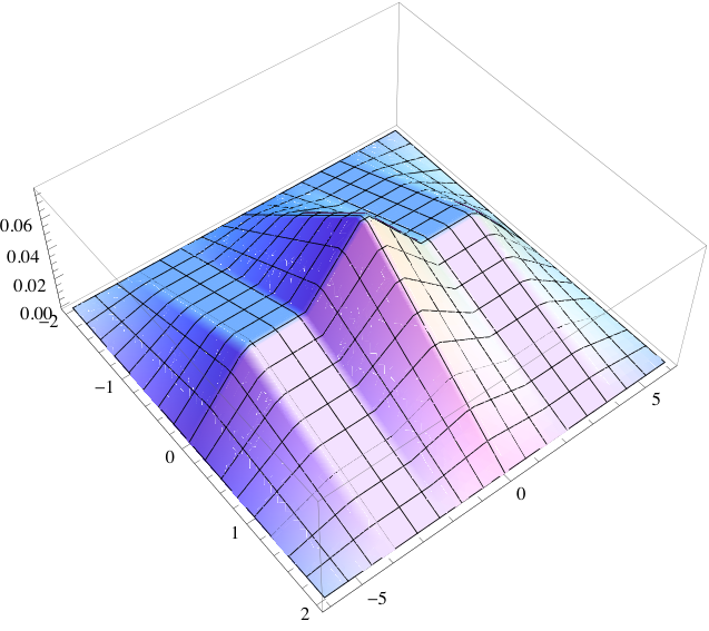
It is also worth noting the following difference between the situation in one dimension and the result for preservation of convolution in higher dimensions: as we note following Theorems 29 and 33, Ibragimov [1956a] and Keilson and Gerber [1971] showed that in the one-dimensional continuous and discrete settings respectively that if $p\star q$ is unimodal for every unimodal $q$ , then $p$ is log-concave. The analogue of this for $d>1$ is more complicated in part because of the great variety of possible definitions of “unimodal” in this case; see Dharmadhikari and Joag-Dev [1988] chapters 2 and 3 for a thorough discussion. In particular Sherman [1955] provided the following counterexample when the notion of unimodality is taken to be centrally symmetric convex unimodality; that is, the sets $S_{c}(p)\equiv\{x\in\mathbb{R}^{d}:p(x)\geq c\}$ are symmetric and convex for each $c\geq 0$ . Let $p$ be the uniform density on $[-1,1]^{2}$ (so that $p(x)=(1/4)1_{[-1,1]^{2}}(x)$ ); then $p$ is log-concave. Let $q$ be the density given by $1/12$ on $[-1,1]^{2}$ and $1/24$ on $([-1,1]\times(1,5])\cup([-1,1]\times[-5,-1))$ . Thus $q$ is centrally symmetric convex (and hence also quasi-concave, $q\in\mathcal{P}_{-\infty}$ as in Definition 2.5. But $h=p\star q$ is not centrally symmetric convex (and also is not quasi-concave), since the sets $S_{c}(h)$ are not convex: see Figure 1.

Refer to caption — Fig 1: Sherman’s example, $h=p\star q$

3.1.5 Preservation by (weak) limits

Now we consider preservation of log-concavity under convergence in distribution.

Proposition 3.6.

(log-concavity is preserved under convergence in distribution). Suppose that $\{P_{n}\}$ is a sequence of log-concave probability measures on $\mathbb{R}^{d}$ , and suppose that $P_{n}\rightarrow_{d}P_{0}$ . Then $P_{0}$ is a log-concave probability measure.

Proof.

See Dharmadhikari and Joag-Dev [1988], Theorem 2.10, page 53. ∎

Note that the limit measure in Proposition 3.6 might be concentrated on a proper subspace of $\mathbb{R}^{d}$ . If we have a sequence of log-concave densities $p_{n}$ which converge pointwise to a density function $p_{0}$ , then by Scheffé’s theorem we have $p_{n}\rightarrow p_{0}$ in $L_{1}(\lambda)$ and hence $d_{TV}(P_{n},P_{0})\rightarrow 0$ . Since convergence in total variation implies convergence in distribution we conclude that $P_{0}$ is a log-concave measure where the affine hull of $\mbox{supp}(P_{0})$ has dimension $d$ and hence $P_{0}$ is the measure corresponding to $p_{0}$ which is necessarily log-concave by Theorem 2.7.

Recall that the class of normal distributions on $\mathbb{R}^{d}$ is closed under all the operations discussed above: affine transformation, formation of products, marginalization, convolution, and weak limits. Since the larger class of log-concave distributions on $\mathbb{R}^{d}$ is also preserved under these operations, the preservation results of this section suggest that the class of log-concave distributions is a very natural nonparametric class which can be viewed naturally as an enlargement of the class of all normal distributions. This has stimulated much recent work on nonparametric estimation for the class of log-concave distributions on $\mathbb{R}$ and $\mathbb{R}^{d}$ : for example, see Dümbgen and Rufibach [2009], Cule and Samworth [2010], Cule, Samworth and Stewart [2010], Walther [2009], Balabdaoui, Rufibach and Wellner [2009], and Henningsson and Astrom [2006], and see Section 9.13 for further details.

3.2 Preservation of strong log-concavity

Here is a theorem summarizing several preservation results for strong log-concavity. Parts (a), (b), and (d) were obtained by Henningsson and Astrom [2006].

Theorem 3.7.

(Preservation of strong log-concavity)
(a) (Linear transformations) Suppose that $X$ has density $p\in SLC_{2}(0,\Sigma,d)$ and let $A$ be a $d\times d$ nonsingular matrix. Then $Y=AX$ has density $q\in SLC_{2}(0,A\Sigma A^{T},d)$ given by $q(y)=p(A^{-1}y)\mbox{det}(A^{-1})$ .
(b) (Convolution) If $Z=X+Y$ where $X\sim p\in SLC_{2}(0,\Sigma,d)$ and $Y\sim q\in SLC_{2}(0,\Gamma,d)$ are independent, then $Z=X+Y\sim p\star q\in SLC_{2}(0,\Sigma+\Gamma,d)$ .
(c) (Product distribution) If $X\sim p\in SLC_{2}(0,\Sigma,m)$ and $Y\sim q\in SLC_{2}(0,\Gamma,n)$ , then

(X,Y)\sim p\cdot q\in SLC_{2}\left(0,\left(\begin{array}[]{cc}\Sigma&0\\ 0&\Gamma\end{array}\right),m+n\right).

(d) (Product function) If $p\in SLC_{2}(0,\Sigma,d)$ and $q\in SLC_{2}(0,\Gamma,d)$ , then $h$ given by $h(x)=p(x)q(x)$ (which is typically not a probability density function) satisfies $h\in SLC_{2}(0,(\Sigma^{-1}+\Gamma^{-1})^{-1})$ .

Part (b) of Theorem 3.7 is closely related to the following result which builds upon and strengthens Prékopa’s Theorem 3.3. It is due to Brascamp and Lieb [1976] (Theorem 4.3, page 380); see also Simon [2011], Theorem 13.13, page 204.

Theorem 3.8.

(Preservation of strong log-concavity under marginalization). Suppose that $p\in SLC_{2}(0,\Sigma,m+n)$ . Then the marginal density $q$ on $\mathbb{R}^{n}$ given by

\displaystyle q(x)=\int_{\mathbb{R}^{m}}p(x,y)dy

is strongly log-concave: $q\in SLC_{2}(0,\Sigma_{11},m)$ where

\displaystyle\Sigma=\left(\begin{array}[]{cc}\Sigma_{11}&\Sigma_{12}\\ \Sigma_{21}&\Sigma_{22}\end{array}\right).

Proof.

Since $p\in SLC_{2}(0,\Sigma,m+n)$ we can write

	$\displaystyle p(x,y)$	$\displaystyle=$	$\displaystyle g(x,y)\phi_{\Sigma}(x,y)$
		$\displaystyle=$	$\displaystyle g(x,y)\frac{1}{(2\pi\|\Sigma\|)^{(m+n)/2}}\exp\left(-\frac{1}{2}(x^{T},y^{T})\left(\begin{array}[]{cc}\Sigma_{11}&\Sigma_{12}\\ \Sigma_{21}&\Sigma_{22}\end{array}\right)^{-1}\left(\begin{array}[]{c}x\\ y\end{array}\right)\right)$

where $g$ is log-concave. Now the Gaussian term in the last display can be written as

$\displaystyle\phi_{Y\|X}(y\|x)\cdot\phi_{X}(x)$
	$\displaystyle=$	$\displaystyle\frac{1}{(2\pi\|\Sigma_{22\cdot 1}\|)^{n/2}}\exp\left(-\frac{1}{2}(y-\Sigma_{21}\Sigma_{11}^{-1}x)^{T}\Sigma_{22\cdot 1}^{-1}(y-\Sigma_{21}\Sigma_{11}^{-1}x)\right)$
		$\displaystyle\ \ \ \cdot\frac{1}{(2\pi\|\Sigma_{11}\|)^{m/2}}\exp\left(-\frac{1}{2}x^{T}\Sigma_{11}^{-1}x\right)$

where $\Sigma_{22\cdot 1}\equiv\Sigma_{22}-\Sigma_{21}\Sigma_{11}^{-1}\Sigma_{12}$ , and hence

$\displaystyle q(x)$	$\displaystyle=$	$\displaystyle\int_{\mathbb{R}^{n}}g(x,y)\frac{1}{(2\pi\|\Sigma_{22\cdot 1}\|)^{n/2}}\exp\left(-\frac{1}{2}(y-\Sigma_{21}\Sigma_{11}^{-1}x)^{T}\Sigma_{22\cdot 1}^{-1}(y-\Sigma_{21}\Sigma_{11}^{-1}x)\right)dy$
		$\displaystyle\ \ \ \cdot\frac{1}{(2\pi\|\Sigma_{11}\|)^{m/2}}\exp\left(-\frac{1}{2}x^{T}\Sigma_{11}^{-1}x\right)$
	$\displaystyle=$	$\displaystyle\int_{\mathbb{R}^{n}}g(x,\tilde{y}+\Sigma_{21}\Sigma_{11}^{-1}x)\cdot\frac{1}{(2\pi\|\Sigma_{22\cdot 1}\|)^{n/2}}\exp\left(-\frac{1}{2}\tilde{y}^{T}\Sigma_{22\cdot 1}^{-1}\tilde{y}\right)d\tilde{y}$
		$\displaystyle\ \ \ \cdot\frac{1}{(2\pi\|\Sigma_{11}\|)^{m/2}}\exp(-(1/2)x^{T}\Sigma_{11}^{-1}x)$
	$\displaystyle\equiv$	$\displaystyle h(x)\phi_{\Sigma_{11}}(x)$

where

\displaystyle h(x)\equiv\int_{\mathbb{R}^{n}}g(x,\tilde{y}+\Sigma_{21}\Sigma_{11}^{-1}x)\cdot\frac{1}{(2\pi|\Sigma_{22\cdot 1}|)^{n/2}}\exp\left(-\frac{1}{2}\tilde{y}^{T}\Sigma_{22\cdot 1}^{-1}\tilde{y}\right)d\tilde{y}

is log-concave: $g$ is log-concave, and hence $\tilde{g}(x,\tilde{y})\equiv g(x,\tilde{y}+\Sigma_{21}\Sigma_{11}^{-1}x)$ is log-concave; the product $\tilde{g}(x,\tilde{y})\cdot\exp(-(1/2)\tilde{y}^{T}\Sigma_{22\cdot 1}^{-1}\tilde{y})$ is (jointly) log-concave; and hence $h$ is log-concave by Prékopa’s Theorem 3.3. ∎

Proof.

(Theorem 3.7): (a) The density $q$ is given by $q(y)=p(A^{-1}y)\det(A^{-1})$ by a standard computation. Then since $p\in SLC_{2}(0,\Sigma,d)$ we can write

\displaystyle q(y)=g(A^{-1}y)\det(A^{-1})\phi_{\Sigma}(A^{-1}y)=g(A^{-1}y)\phi_{A\Sigma A^{T}}(y)

where $g(A^{-1}y)$ is log-concave by Proposition 3.1.
(b) If $p\in SLC_{2}(0,\Sigma,d)$ and $q\in SLC_{2}(0,\Gamma,d)$ , then the function

\displaystyle h(z,x)=p(x)q(z-x)

is strongly log-concave jointly in $x$ and $z$ : since

	$\displaystyle x^{T}\Sigma^{-1}x+(z-x)^{T}\Gamma^{-1}(z-x)$
		$\displaystyle=$	$\displaystyle z^{T}(\Sigma+\Gamma)^{-1}z+(x-Cz)^{T}(\Sigma^{-1}+\Gamma^{-1})(x-Cz)$

where $C\equiv(\Sigma^{-1}+\Gamma^{-1})^{-1}\Gamma^{-1}$ , it follows that

	$\displaystyle h(z,x)$	$\displaystyle=$	$\displaystyle g_{p}(x)g_{q}(z-x)\phi_{\Sigma}(x)\phi_{\Gamma}(z-x)$
		$\displaystyle=$	$\displaystyle g(z,x)\phi_{\Sigma+\Gamma}(z)\cdot\phi_{\Sigma^{-1}+\Gamma^{-1}}(x-Cz)$

is jointly log-concave. Hence it follows that

	$\displaystyle p\star q(z)=\int_{\mathbb{R}^{d}}h(z,x)dx$	$\displaystyle=$	$\displaystyle\phi_{\Sigma+\Gamma}(z)\int_{\mathbb{R}^{d}}g(z,x)\phi_{\Sigma^{-1}+\Gamma^{-1}}(x-Cz)dx$
		$\displaystyle\equiv$	$\displaystyle\phi_{\Sigma+\Gamma}(z)g_{0}(z)$

where $g_{0}(z)$ is log-concave by Prékopa’s theorem, Theorem 3.3.
(c ) This is easy since

\displaystyle p(x)q(y)

\displaystyle=

\displaystyle g_{p}(x)g_{q}(y)\phi_{\Sigma}(x)\phi_{\Gamma}(y)=g(x,y)\phi_{\tilde{\Sigma}}(x,y)

where $\tilde{\Sigma}$ is the given $2d\times 2d$ block diagonal matrix and $g$ is jointly log-concave (by Proposition 3.2).
(d) Note that

\displaystyle p(x)q(x)=g_{p}(x)g_{q}(x)\phi_{\Sigma}(x)\cdot\phi_{\Gamma}(x)\equiv g_{0}(x)\phi_{(\Sigma^{-1}+\Gamma^{-1})^{-1}}(x)

where $g_{0}$ is log-concave. ∎

4 Log-concavity and ultra-log-concavity for discrete distributions

We now consider log-concavity and ultra-log-concavity in the setting of discrete random variables. Some of this material is from Johnson, Kontoyiannis and Madiman [2013] and Johnson [2007].

An integer-valued random variable $X$ with probability mass function $\{p_{x}:\ x\in\mathbb{Z}\}$ is log-concave if

\displaystyle p_{x}^{2}\geq p_{x+1}p_{x-1}\ \ \mbox{for all}\ x\in\mathbb{Z}.

(4.9)

If we define the score function $\varphi$ by $\varphi(x)\equiv p_{x+1}/p_{x}$ , then log-concavity of $\{p_{x}\}$ is equivalent to $\varphi$ being decreasing (nonincreasing).

A stronger notion, analogous to strong log-concavity in the case of continuous random variables, is that of ultra-log-concavity: for any $\lambda>0$ define $\mathbf{ULC}(\lambda)$ to be the class of integer-valued random variables $X$ with mean $EX=\lambda$ such that the probability mass function $p_{x}$ satisfies

\displaystyle xp_{x}^{2}\geq(x+1)p_{x+1}p_{x-1}\ \ \ \mbox{for all}\ \ x\geq 1.

(4.10)

Then the class of ultra log-concave random variables is $\mathbf{ULC}=\cup_{\lambda>0}\mathbf{ULC}(\lambda)$ . Note that (4.10) is equivalent to log-concavity of $x\mapsto p_{x}/\pi_{\lambda,x}$ where $\pi_{\lambda,x}=e^{-\lambda}\lambda^{x}/x!$ is the Poisson distribution on $\mathbb{N}$ , and hence ultra-log-concavity corresponds to $p$ being log-concave relative to $\pi_{\lambda}$ (or $p\leq_{{\small\mbox{lc}}}\pi_{\lambda}$ ) in the sense defined by Whitt [1985]. Equivalently, $p_{x}=h_{x}\pi_{\lambda,x}$ where $h$ is log-concave. When we want to emphasize that the mass function $\{p_{x}\}$ corresponds to $X$ , we also write $p_{X}(x)$ instead of $p_{x}$ .

If we define the relative score function $\rho$ by

\displaystyle\rho(x)

\displaystyle\equiv

\displaystyle\frac{(x+1)p_{x+1}}{\lambda p_{x}}-1,

then $X\sim p\in\mathbf{ULC}(\lambda)$ if and only if $\rho$ is decreasing (nonincreasing). Note that

\rho(x)=\frac{(x+1)\varphi(x)}{\lambda}-1=\frac{(x+1)\varphi(x)}{\lambda}-\frac{(x+1)\pi_{\lambda,x+1}}{\lambda\pi_{\lambda,x}}.

Our main interest here is the preservation of log-concavity and ultra-log-concavity under convolution.

Theorem 4.1.

(a) (Keilson and Gerber [1971]) The class of log-concave distributions on $\mathbb{Z}$ is closed under convolution. If $U\sim p$ and $V\sim q$ are independent and $p$ and $q$ are log-concave, then $U+V\sim p\star q$ is log-concave.
(b) (Walkup [1976], Liggett [1997]) The class of ultra-log-concave distributions on $\mathbb{Z}$ is closed under convolution. More precisely, these classes are closed under convolution in the following sense: if $U\in\mathbf{ULC}(\lambda)$ and $V\in\mathbf{ULC}(\mu)$ are independent, then $U+V\in\mathbf{ULC}(\lambda+\mu)$ .

Actually, Keilson and Gerber [1971] proved more: analogously to Ibragimov [1956a] they showed that $p$ is strongly unimodal (i.e. $X+Y\sim p\star q$ with $X,Y$ independent is unimodal for every unimodal $q$ on $\mathbb{Z}$ ) if and only if $X\sim p$ is log-concave. Liggett’s proof of (b) proceeds by direct calculation; see also Walkup [1976]. For recent alternative proofs of this property of ultra-log-concave distributions, see Gurvits [2009] and Kahn and Neiman [2011]. A relatively simple proof is given by Johnson [2007] using results from Kontoyiannis, Harremoës and Johnson [2005] and Efron [1965], and that is the proof we will summarize here. See Nayar and Oleszkiewicz [2012] for an application of ultra log-concavity and Theorem 4.1 to finding optimal constants in Khinchine inequalities.

Before proving Theorem 4.1 we need the following lemma giving the score and the relative score of a sum of independent integer-valued random variables.

Lemma 4.2.

If $X,Y$ are independent non-negative integer-valued random variables with mass functions $p=p_{X}$ and $q=p_{Y}$ then:
(a) $\varphi_{X+Y}(z)=E\{\varphi_{X}(X)|X+Y=z\}$ .
(b) If, moreover, $X$ and $Y$ have means $\mu$ and $\nu$ respectively, then with $\alpha=\mu/(\mu+\nu)$ ,

\displaystyle\rho_{X+Y}(z)=E\{\alpha\rho_{X}(X)+(1-\alpha)\rho_{Y}(Y)\big|X+Y=z\}.

Proof.

For (a), note that with $F_{z}\equiv p_{X+Y}(z)$ we have

$\displaystyle\varphi_{X+Y}(z)$	$\displaystyle=$	$\displaystyle\frac{p_{X+Y}(z+1)}{p_{X+Y}(z)}=\sum_{x}\frac{p(x)q(z+1-x)}{F_{z}}$
	$\displaystyle=$	$\displaystyle\sum_{x}\frac{p(x)}{p(x-1)}\cdot\frac{p(x-1)q(z+1-x)}{F_{z}}$
	$\displaystyle=$	$\displaystyle\sum_{x}\frac{p(x+1)}{p(x)}\cdot\frac{p(x)q(z-x)}{F_{z}}.$

To prove (b) we follow Kontoyiannis, Harremoës and Johnson [2005], page 471: using the same notation as in (a),

$\displaystyle\rho_{X+Y}(z)$	$\displaystyle=$	$\displaystyle\frac{(z+1)p_{X+Y}(z+1)}{(\mu+\nu)p_{X+Y}(z)}-1$
	$\displaystyle=$	$\displaystyle\sum_{x}\frac{(z+1)p(x)q(z+1-x)}{(\mu+\nu)F_{z}}-1$
	$\displaystyle=$	$\displaystyle\sum_{x}\left\{\frac{xp(x)q(z+1-x)}{(\mu+\nu)F_{z}}\ +\ \frac{(z-x+1)p(x)q(z+1-x)}{(\mu+\nu)F_{z}}\right\}-1$
	$\displaystyle=$	$\displaystyle\alpha\left\{\sum_{x}\frac{xp_{X}(x)}{\mu p(x-1)}\cdot\frac{p(x-1)q(z-x+1)}{F_{z}}-1\right\}$
		$\displaystyle\ \ \ +\ (1-\alpha)\left\{\sum_{x}\frac{z-x+1}{\nu}\frac{q(z-x+1)}{q(z-x)}\cdot\frac{p(x)q(z-x)}{F_{z}}-1\right\}$
	$\displaystyle=$	$\displaystyle\sum_{x}\frac{p(x)q(z-x)}{F_{z}}\left\{\alpha\rho_{X}(x)+(1-\alpha)\rho_{Y}(z-x)\right\}.$

∎

Proof.

Theorem 4.1: (b) This follows from (b) of Lemma 4.2 and Theorem 1 of Efron [1965], upon noting Efron’s remark 1, page 278, concerning the discrete case of his theorem: for independent log-concave random variables $X$ and $Y$ and a measurable function $\Phi$ monotone (decreasing here) in each argument, $E\{\Phi(X,Y)|X+Y=z\}$ is a monotone decreasing function of $z$ : note that log-concavity of $X$ and $Y$ implies that

\Phi(x,y)=\frac{\mu}{\mu+\nu}\rho_{X}(x)+\frac{\nu}{\mu+\nu}\rho_{Y}(y)

is a monotone decreasing function of $x$ and $y$ (separately) by since the relative scores $\rho_{X}$ and $\rho_{Y}$ are decreasing. Thus $\rho_{X+Y}$ is a decreasing function of $z$ , and hence $X+Y\in\mathbf{ULC}(\mu+\nu)$ .

(a) Much as in part (b), this follows from (a) of Lemma 4.2 and Theorem 1 of Efron [1965], upon replacing the relative scores $\rho_{X}$ and $\rho_{Y}$ by scores $\varphi_{X}$ and $\varphi_{Y}$ and by taking $\Phi(x,y)=\varphi_{X}(x)$ . ∎

For interesting results concerning the entropy of discrete random variables, Bernoulli sums, log-concavity, and ultra-log-concavity, see Johnson, Kontoyiannis and Madiman [2013], Ehm [1991], and Johnson [2007]. For recent results concerning nonparametric estimation of a discrete log-concave distribution, see Balabdaoui et al. [2013] and Balabdaoui [2014]. It follows from Ehm [1991] that the hypergeometric distribution (sampling without replacement count of “successes”) is equal in distribution to a Bernoulli sum; hence the hypergeometric distribution is ultra-log-concave.

5 Regularity and approximations of log-concave functions

5.1 Regularity

The regularity of a log-concave function $f=\exp\left(-\varphi\right)$ depends on the regularity of its convex potential $\varphi$ . Consequently, log-concave functions inherit the special regularity properties of convex functions.

Any log-concave function is nonnegative. When the function $f$ is a log-concave density (with respect to the Lebesgue measure), which means that $f$ integrates to $1$ , then it is automatically bounded. More precisely, it has exponentially decreasing tails and hence, it has finite $\Psi_{1}$ Orlicz norms; for example, see Borell [1983] and Ledoux [2001]. The following lemma gives a pointwise estimate of the density.

Theorem 5.1 (Cule and Samworth [2010], Lemma 1).

Let $f$ be a log-concave density on $\mathbb{R}^{d}$ . Then there exist $a_{f}=a>0$ and $b_{f}=b\in\mathbb{R}$ such that $f\left(x\right)\leq e^{-a\left\|x\right\|+b}$ for all $x\in\mathbb{R}^{d}$ .

Similarly, strong log-concavity implies a finite $\Psi_{2}$ Orlicz norm (see Ledoux [2001] Theorem 2.15, page 36, Villani [2003], Theorem 9.9, page 280), Bobkov [1999], and Bobkov and Götze [1999].

For other pointwise bounds on log-concave densities themselves, see Devroye [1984], Dümbgen and Rufibach [2009] and Lovász and Vempala [2007].

As noticed in Cule and Samworth [2010], Theorem 5.1 implies that if a random vector $X$ has density $f$ , then the moment generating function of $X$ is finite in an open neighborhood of the origin. Bounds can also be obtained for the supremum of a log-concave density as well as for its values on some special points in the case where $d=1$ .

Proposition 5.2.

Let $X$ be a log-concave random variable, with density $f$ on $\mathbb{R}$ and median $m$ . Then

$\displaystyle\frac{1}{12\var\left(X\right)}$	$\displaystyle\leq$	$\displaystyle f\left(m\right)^{2}\leq\frac{1}{2\var\left(X\right)}\text{ ,}$	(5.11)
$\displaystyle\frac{1}{12\var\left(X\right)}$	$\displaystyle\leq$	$\displaystyle\sup_{x\in\mathbb{R}}f\left(x\right)^{2}\leq\frac{1}{\var\left(X\right)}\text{ ,}$	(5.12)
$\displaystyle\frac{1}{3e^{2}\var\left(X\right)}$	$\displaystyle\leq$	$\displaystyle f\left(\mathbb{E}\left[X\right]\right)^{2}\leq\frac{1}{\var\left(X\right)}\text{ .}$	(5.13)

Proposition 5.2 can be found in Bobkov and Ledoux [2014], Proposition B.2. See references therein for historical remarks concerning these inequalities. Proposition 5.2 can also be seen as providing bounds for the variance of a log-concave variable. See Kim and Samworth [2014], section 3.2, for some further results of this type.

Notice that combining (5.11) and (5.12) we obtain the inequality $\sup_{x\in\mathbb{R}}f\left(x\right)\leq 2\sqrt{3}f\left(m\right)$ . In fact, the concavity of the function $I$ defined in Proposition 2.21 allows to prove the stronger inequality $\sup_{x\in\mathbb{R}}f\left(x\right)\leq 2f\left(m\right)$ . Indeed, with the notations of Proposition 2.21, we have $I\left(1/2\right)=f\left(m\right)$ and for any $x\in\left(a,b\right)$ , there exists $t\in\left(0,1\right)$ such that $x=F^{-1}\left(t\right)$ . Hence,

	$\displaystyle 2f\left(m\right)=2I\left(\frac{1}{2}\right)=2I\left(\frac{t}{2}+\frac{1-t}{2}\right)$
		$\displaystyle\geq$	$\displaystyle 2\left(\frac{1}{2}I\left(t\right)+\frac{1}{2}I\left(1-t\right)\right)\geq I\left(t\right)=f\left(x\right)\text{ .}$

A classical result on continuity of convex functions is that any real-valued convex function $\varphi$ defined on an open set $U\subset\mathbb{R}^{d}$ is locally Lipschitz and in particular, $\varphi$ is continuous on $U$ . For more on continuity of convex functions see Section 3.5 of Niculescu and Persson [2006]. Of course, any continuity of $\varphi$ (local or global) corresponds to the same continuity of $f$ .

For an exposé on differentiability of convex functions, see Niculescu and Persson [2006] (in particular sections 3.8 and 3.11; see also Alberti and Ambrosio [1999] section 7). A deep result of Alexandroff [1939] is the following (we reproduce here Theorem 3.11.2 of Niculescu and Persson [2006]).

Theorem 5.3 (Alexandroff [1939]).

Every convex function $\varphi$ on $\mathbb{R}^{d}$ is twice differentiable almost everywhere in the following sense: $f$ is twice differentiable at a, with Alexandrov Hessian $\nabla^{2}f\left(a\right)$ in $\Sym^{+}\left(d,\mathbb{R}\right)$ (the space of real symmetric $d\times d$ matrices), if $\nabla f\left(a\right)$ exists, and if for every $\varepsilon>0$ there exists $\delta>0$ such that

\left\|x-a\right\|<\delta\text{ \ \ implies \ \ }\sup_{y\in\partial f\left(x\right)}\left\|y-\nabla f\left(a\right)-\nabla^{2}f\left(a\right)\left(x-a\right)\right\|\leq\varepsilon\left\|x-a\right\|\text{ .}

Here $\partial f\left(x\right)$ is the subgradient of $f$ at $x$ (see Definition 8.3 in Rockafellar and Wets [1998]). Moreover, if $a$ is such a point, then

\lim_{h\rightarrow 0}\frac{f\left(a+h\right)-f\left(a\right)-\left\langle\nabla f\left(a\right),h\right\rangle-\frac{1}{2}\left\langle\nabla^{2}f\left(a\right)h,h\right\rangle}{\left\|h\right\|^{2}}=0\text{ .}

We immediately see by Theorem 5.3, that since $\varphi$ is convex and $f=\exp\left(-\varphi\right)$ , it follows that $f$ is almost everywhere twice differentiable. For further results in the direction of Alexandrov’s theorem see Dudley [1977]; Dudley [1980].

5.2 Approximations

Again, if one wants to approximate a non-smooth log-concave function $f=\exp\left(-\varphi\right)$ by a sequence of smooth log-concave functions, then convexity of the potential $\varphi$ can be used to advantage. For an account about approximation of convex functions see Niculescu and Persson [2006], section 3.8.

On the one hand, if $\varphi\in L_{loc}^{1}\left(\mathbb{R}^{d}\right)$ the space of locally integrable functions, then the standard use of a regularization kernel (i.e. a one-parameter family of functions associated with a mollifier) to approximate $\varphi$ preserves the convexity as soon as the mollifier is nonnegative. A classical result is that this gives in particular approximations of $\varphi$ in $L^{p}$ spaces, $p\geq 1$ , as soon as $\varphi\in L^{p}\left(\mathbb{R}^{d}\right)$ .

On the other hand, infimal convolution (also called epi-addition, see Rockafellar and Wets [1998]) is a nonlinear analogue of mollification that gives a way to approximate a lower semicontinuous proper convex function from below (section 3.8, Niculescu and Persson [2006]). More precisely, take two proper convex functions $f$ and $g$ from $\mathbb{R}^{d}$ to $\mathbb{R}\cup\left\{\infty\right\}$ , which means that the functions are convex and finite for at least one point. The infimal convolution between $f$ and $g$ , possibly taking the value $-\infty$ , is

\left(f\odot g\right)\left(x\right)=\inf_{y\in\mathbb{R}^{n}}\left\{f\left(x-y\right)+g\left(y\right)\right\}\text{ .}

Then, $f\odot g$ is a proper convex function as soon as $f\odot g\left(x\right)>-\infty$ for all $x\in\mathbb{R}^{d}$ . Now, if $f$ is a lower semicontinuous proper convex function on $\mathbb{R}^{d}$ , the Moreau-Yosida approximation $f_{\varepsilon}$ of $f$ is given by

	$\displaystyle f_{\varepsilon}\left(x\right)$	$\displaystyle=$	$\displaystyle\left(f\odot\frac{1}{2\varepsilon}\left\\|\cdot\right\\|^{2}\right)\left(x\right)$
		$\displaystyle=$	$\displaystyle\inf_{y\in\mathbb{R}^{n}}\left\{f\left(y\right)+\frac{1}{2\varepsilon}\left\\|x-y\right\\|^{2}\right\}\text{ .}$

for any $x\in\mathbb{R}^{d}$ and $\varepsilon>0$ . The following theorem can be found in Alberti and Ambrosio [1999] (Proposition 7.13), see also Barbu and Precupanu [1986], Brézis [1973] or Niculescu and Persson [2006].

Theorem 5.4.

The Moreau-Yosida approximates $f_{\varepsilon}$ are $\mathcal{C}^{1,1}$ (i.e. differentiable with Lipschitz derivative) convex functions on $\mathbb{R}^{d}$ and $f_{\varepsilon}\rightarrow f$ as $\varepsilon\rightarrow 0$ . Moreover, $\partial f_{\varepsilon}=\left(\varepsilon I+\left(\partial f\right)^{-1}\right)^{-1}$ as set-valued maps.

An interesting consequence of Theorem 5.4 is that if two convex and proper lower semicontinuous functions agree on their subgradients, then they are equal up to a constant (corollary 2.10 in Brézis [1973]).

Approximation by a regularization kernel and Moreau-Yosida approximation have different benefits. While a regularization kernel gives the most differentiability, the Moreau-Yosida approximation provides an approximation of a convex function from below (and so, a log-concave function from above). It is thus possible to combine these two kinds of approximations and obtain the advantages of both. For an example of such a combination in the context of a (multivalued) stochastic differential equation and the study of the so-called Kolmogorov operator, see Barbu and Da Prato [2008].

When considering a log-concave random vector, the following simple convolution by Gaussian vectors gives an approximation by log-concave vectors that have $\mathcal{C}^{\infty}$ densities and finite Fisher information matrices. In the context of Fisher information, regularization by Gaussians was used for instance in Port and Stone [1974] to study the Pitman estimator of a location parameter.

Proposition 5.5 (convolution by Gaussians).

Let $X$ be a random vector in $\mathbb{R}^{d}$ with density $p$ w.r.t. the Lebesgue measure and $G$ a $d$ -dimensional standard Gaussian variable, independent of $X$ . Set $Z=X+\sigma G$ , $\sigma>0$ and $p_{Z}=\exp\left(-\varphi_{Z}\right)$ the density of $Z$ . Then:

(i)

If $X$ is log-concave, then $Z$ is also log-concave.

(ii)

If $X$ is strongly log-concave, $Z\in SLC_{1}\left(\tau^{2},d\right)$ then $Z$ is also strongly log-concave; $Z\in SLC_{1}\left(\tau^{2}+\sigma^{2},d\right)$ .

(iii)

$Z$ has a positive density $p_{Z}$ on $\mathbb{R}^{d}$ . Furthermore, $\varphi_{Z}$ is $C^{\infty}$ on $\mathbb{R}^{d}$ and

	$\displaystyle\nabla\varphi_{Z}\left(z\right)$	$\displaystyle=$	$\displaystyle\sigma^{-2}\mathbb{E}\left[\sigma G\left\|X+\sigma G=z\right.\right]$		(5.14)
		$\displaystyle=$	$\displaystyle\mathbb{E}\left[\rho_{\sigma G}\left(\sigma G\right)\left\|X+\sigma G=z\right.\right]\text{ ,}$		(5.14)

where $\rho_{\sigma G}\left(x\right)=\sigma^{-2}x$ is the score of $\sigma G$ .

(iv)

The Fisher information matrix for location $J(Z)=\mathbb{E}\left[\nabla\varphi_{Z}\otimes\nabla\varphi_{Z}\left(Z\right)\right]$ , is finite and we have $J\left(Z\right)\leq J\left(\sigma G\right)=\sigma^{-4}I_{d}$ as symmetric matrices.

Proof.

See Section 11. ∎

We now give a second approximation tool, that allows to approximate any log-concave density by strongly log-concave densities.

Proposition 5.6.

Let $f$ be a log-concave density on $\mathbb{R}^{d}$ . Then for any $c>0$ , the density

h_{c}\left(x\right)=\frac{f\left(x\right)e^{-c\left\|x\right\|^{2}/2}}{\int_{\mathbb{R}^{d}}f\left(v\right)e^{-c\left\|v\right\|^{2}/2}dv},\text{ \ \ }x\in\mathbb{R}^{d},

is $SLC_{1}\left(c^{-1},d\right)$ and $h_{c}\rightarrow f$ as $c\rightarrow 0$ in $L_{p}$ , $p\in\left[1,\infty\right]$ . More precisely, there exists a constant $A_{f}>0$ depending only on $f$ , such that for any $\varepsilon>0$ ,

\sup\left\{\sup_{x\in\mathbb{R}^{d}}\left|h_{c}\left(x\right)-f\left(x\right)\right|;\left(\int_{\mathbb{R}^{d}}\left|h_{c}\left(x\right)-f\left(x\right)\right|^{p}dx\right)^{1/p}\right\}\leq A_{f}c^{1-\varepsilon}\text{ .}

Proof.

See Section 11. ∎

Finally, by combining Proposition 5.6 and 5.5, we obtain the following approximation lemma.

Proposition 5.7.

For any log-concave density on $\mathbb{R}^{d}$ , there exists a sequence of strongly log-concave densities that are $\mathcal{C}^{\infty}$ , have finite Fisher information matrices and that converge to $f$ in $L_{p}\left(\leb\right)$ , $p\in\left[1,\infty\right]$ .

Proof.

Approximate $f$ by a strongly log-concave density $h$ as in Proposition 5.6. Then approximate $h$ by convolving with a Gaussian density. In the two steps the approximations can be as tight as desired in $L_{p}$ , for any $p\in\left[1,\infty\right]$ . The fact that the convolution with Gaussians for a (strongly) log-concave density (that thus belongs to any $L_{p}\left(\leb\right)$ , $p\in\left[1,\infty\right]$ ) gives approximations in $L_{p}$ , $p\in\left[1,\infty\right]$ is a simple application of general classical theorems about convolution in $L_{p}$ (see for instance Rudin [1987], p. 148). ∎

6 Efron’s theorem and more on preservation of log-concavity and strong log-concavity under convolution in 1-dimension

Another way of proving that strong log-concavity is preserved by convolution in the one-dimensional case is by use of a result of Efron [1965]. This has already been used by Johnson, Kontoyiannis and Madiman [2013] and Johnson [2007] to prove preservation of ultra log-concavity under convolution (for discrete random variables), and by Wellner [2013] to give a proof that strong log-concavity is preserved by convolution in the one-dimensional continuous setting. These proofs operate at the level of scores or relative scores and hence rely on the equivalences between (a) and (b) in Propositions 2.20 and 2.23. Our goal in this section is to re-examine Efron’s theorem, briefly revisit the results of Johnson, Kontoyiannis and Madiman [2013] and Wellner [2013], give alternative proofs using second derivative methods via symmetrization arguments, and to provide a new proof of Efron’s theorem using some recent results concerning asymmetric Brascamp-Lieb inequalities due to Menz and Otto [2013] and Carlen, Cordero-Erausquin and Lieb [2013].

6.1 Efron’s monotonicity theorem

The following monotonicity result is due to Efron [1965].

Theorem 6.1 (Efron).

Suppose that $\Phi:\mathbb{R}^{m}\rightarrow\mathbb{R}$ where $\Phi$ is coordinatewise non-decreasing and let

g(z)\equiv E\left\{\Phi(X_{1},\cdots,X_{m})\bigg|\sum_{j=1}^{m}X_{j}=z\right\},

where $X_{1},\ldots,X_{m}$ are independent and log-concave. Then $g$ is non-decreasing.

Remark 6.2.

As noted by Efron [1965], Theorem 6.1 continues to hold for integer valued random variables which are log-concave in the sense that $p_{x}\equiv P(X=x)$ for $x\in\mathbb{Z}$ satisfies $p_{x}^{2}\geq p_{x+1}p_{x-1}$ for all $x\in\mathbb{Z}$ .

In what follows, we will focus on Efron’s theorem for $m=2$ . As it is shown in Efron [1965], the case of a pair of variables ( $m=2$ ) indeed implies the general case with $m\geq 2$ . Let us recall the argument behind this fact, which involves preservation of log-concavity under convolution. In fact, stability under convolution for log-concave variables is not needed to prove Efron’s theorem for $m=2$ as will be seen from the new proof of Efron’s theorem given here in Section 6.4, so it is consistent to prove the preservation of log-concavity under convolution via Efron’s theorem for $m=2$ .

Proposition 6.3.

If Theorem 6.1 is satisfied for $m=2$ , then it is satisfied for $m\geq 2$ .

Proof.

We proceed as in Efron [1965] by induction on $m\geq 2$ . Let $\left(X_{1},\ldots,X_{m}\right)$ be a $m-$ tuple of log-concave variables, let $S=\sum_{i=1}^{m}X_{i}$ be their sum and set

\Lambda\left(t,u\right)=\mathbb{E}\left[\Phi\left(X_{1},\ldots,X_{m}\right)\left|\sum_{i=1}^{m-1}X_{i}=t\text{ },\text{ }X_{m}=u\right.\right]\text{ .}

Then

\mathbb{E}\left[\Phi\left(X_{1},\ldots,X_{m}\right)\left|S=s\right.\right]=\mathbb{E}\left[\Lambda\left(T,X_{m}\right)\left|T+X_{m}=s\right.\right]\text{ ,}

where $T=\sum_{i=1}^{m-1}X_{i}$ . Hence, by the induction hypothesis for functions of two variables, it suffices to prove that $\Lambda$ is coordinatewise non-decreasing. As $T$ is a log-concave variable (by preservation of log-concavity by convolution), $\Lambda\left(t,u\right)$ is non-decreasing in $t$ by the induction hypothesis for functions of $m-1$ variables. Also $\Lambda\left(t,u\right)$ is non-decreasing in $u$ since $\Phi$ is non-decreasing in its last argument. ∎

Efron [1965] also gives the following corollaries of Theorem 6.1 above.

Corollary 6.4.

Let $\{\Phi_{t}(x_{1},\ldots,x_{m}):\ t\in T\}$ be a family of measurable functions increasing in every argument for each fixed value of $t$ , and increasing in $t$ for each fixed value of $x_{1},x_{2},\ldots,x_{m}$ . Let $X_{1},\ldots,X_{m}$ be independent and log-concave and write $S\equiv\sum_{j=1}^{m}X_{j}$ . Then

g(a,b)=E\left\{\Phi_{a+b-S}(X_{1},\cdots,X_{m})\bigg|a\leq S\leq a+b\right\}

is increasing in both $a$ and $b$ .

Corollary 6.5.

Suppose that the hypotheses of Theorem 6.1 hold and that $A=\{x=(x_{1},\ldots,x_{m})\in\mathbb{R}^{m}:a_{j}\leq x_{j}\leq b_{j}\}$ with $-\infty\leq a_{j}<b_{j}\leq\infty$ is a rectangle in $\mathbb{R}^{m}$ . Then

g(z)\equiv E\left\{\Phi(X_{1},\cdots,X_{m})\bigg|\sum_{j=1}^{m}X_{j}=z,(X_{1},\ldots,X_{m})\in A\right\}

is a non-decreasing function of $z$ .

The following section will give applications of Efron’s theorem to preservation of log-concavity and strong log-concavity in the case of real-valued variables.

6.2 First use of Efron’s theorem: strong log-concavity is preserved by convolution via scores

Theorem 6.6.

(log-concavity and strong log-concavity preserved by convolution via scores)
(a) (Ibragimov [1956b]) If $X$ and $Y$ are independent and log-concave with densities $p$ and $q$ respectively, then $X+Y\sim p\star q$ is also log-concave.
(b) If $X\in SLC_{1}(\sigma^{2},1)$ and $Y\in SLC_{1}(\tau^{2},1)$ are independent, then $X+Y\in SLC_{1}(\sigma^{2}+\tau^{2},1)$

Actually, Ibragimov [1956b] proved more: he showed that $p$ is strongly unimodal (i.e. $X+Y\sim p\star q$ with $X,Y$ independent is unimodal for every unimodal $q$ on $\mathbb{R}$ ) if and only if $X$ is log-concave.

Proof.

(a) From Proposition 2.20 log-concavity of $p$ and $q$ is equivalent to monotonicity of their score functions $\varphi_{p}^{\prime}=(-\log p)^{\prime}=-p^{\prime}/p$ $a.e.$ and $\varphi_{q}^{\prime}=(-\log q)^{\prime}=-q^{\prime}/q$ $a.e.$ respectively. From the approximation scheme described in Proposition 5.5 above, we can assume that both $p$ and $q$ are absolutely continuous. Indeed, Efron’s theorem applied to formula (5.14) of Proposition 5.5 with $m=2$ and $\Phi(x,y)=\rho_{\sigma G}(x)$ , gives that the convolution with a Gaussian variable preserves log-concavity. Then, from Lemma 3.1 of Johnson and Barron [2004],

E\left\{\rho_{X}(X)\bigg|X+Y=z\right\}=\rho_{X+Y}(z).

Thus by Efron’s theorem with $m=2$ and

\Phi(x,y)=\rho_{Y}(y),

we see that $E\{\Phi(X,Y)|X+Y=z\}=\varphi_{p\star q}^{\prime}(z)$ is a monotone function of $z$ , and hence by Proposition 2.20, (a) if and only if (b), log-concavity of the convolution $p\star q=p_{X+Y}$ holds.

(b) The proof of preservation of strong log-concavity under convolution for $p$ and $q$ strong log-concave on $\mathbb{R}$ is similar to the proof of (a), but with scores replaced by relative scores, but it is interesting to note that a symmetry argument is needed. From Proposition 2.23 strong log-concavity of $p$ and $q$ is equivalent to monotonicity of their relative score functions $\rho_{p}(x)\equiv\varphi_{p}^{\prime}(x)-x/\sigma^{2}$ and $\rho_{q}(x)\equiv\varphi_{q}^{\prime}(x)-x/\tau^{2}$ respectively. Now we take $m=2$ , $\lambda\equiv\sigma^{2}/(\sigma^{2}+\tau^{2})$ , and define

\Phi(x,y)=\lambda\rho_{p}(x)+(1-\lambda)\rho_{q}(y).

Thus $\Phi$ is coordinate-wise monotone and by using Lemma 7.2 with $d=1$ we find that

E\{\Phi(X,Y)|X+Y=z\}=\varphi_{p\star q}^{\prime}(z)-\frac{z}{\sigma^{2}+\tau^{2}}=\rho_{p\star q}(z).

Hence it follows from Efron’s theorem that the relative score $\rho_{p\star q}$ of the convolution $p\star q$ , is a monotone function of $z$ . By Proposition 2.23(b) it follows that $p\star q\in SLC_{1}(\sigma^{2}+\tau^{2},1)$ . ∎

6.3 A special case of Efron’s theorem via symmetrization

We now consider a particular case of Efron’s theorem. Our motivation is as follows: in order to prove that strong log-concavity is preserved under convolution, recall that we need to show monotonicity in $z$ of

\rho_{X+Y}(z)=E\left\{\frac{\sigma^{2}}{\sigma^{2}+\tau^{2}}\rho_{X}(X)+\frac{\tau^{2}}{\sigma^{2}+\tau^{2}}\rho_{Y}(Y)\bigg|X+Y=z\right\}\text{.}

Thus we only need to consider functions $\Phi$ of the form

\Phi(X,Y)=\Psi\left(X\right)+\Gamma\left(Y\right),

where $\Psi$ and $\Gamma$ are non-decreasing, and show the monotonicity of

E\left\{\Phi(X,Y)\bigg|X+Y=z\right\}

for functions $\Phi$ of this special form. By symmetry between $X$ and $Y$ , this reduces to the study of the monotonicity of

E\left\{\Psi\left(X\right)\bigg|X+Y=z\right\}\text{.}

We now give a simple proof of this monotonicity in dimension $1$ .

Proposition 6.7.

Let $\Psi:\mathbb{R\rightarrow R}$ be non-decreasing and suppose that $X\sim f_{X}$ , $Y\sim f_{Y}$ are independent and that $f_{X},f_{Y}$ are log-concave. If the function $\eta:\mathbb{R}\rightarrow\mathbb{R}$ given by

\eta(z)\equiv E\left\{\Psi\left(X\right)\bigg|X+Y=z\right\}

is well-defined ( $\Psi$ integrable with respect to the conditional law of $X+Y$ ), then it is non-decreasing.

Proof.

First notice that by truncating the values of $\Psi$ and using the monotone convergence theorem, we assume that $\Psi$ is bounded. Moreover, by Proposition 5.5, we may assume that $f_{Y}$ is $\mathcal{C}^{1}$ with finite Fisher information, thus justifying the following computations. We write

E\left\{\Psi\left(X\right)\bigg|X+Y=z\right\}=\int_{\mathbb{R}}\Psi\left(x\right)\frac{f_{X}\left(x\right)f_{Y}\left(z-x\right)}{F_{z}}dx\text{ ,}

where

F_{z}=\int_{\mathbb{R}}f_{X}\left(x\right)f_{Y}\left(z-x\right)dx>0\text{ .}

Moreover, with $f_{X}=\exp(-\varphi_{X})$ and $f_{Y}=\exp(-\varphi_{Y})$ ,

$\displaystyle\frac{\partial}{\partial z}\left(\Psi\left(x\right)\frac{f_{X}\left(x\right)f_{Y}\left(z-x\right)}{F_{z}}\right)$
	$\displaystyle=$	$\displaystyle-\Psi\left(x\right)\varphi_{Y}^{\prime}\left(z-x\right)\frac{f_{X}\left(x\right)f_{Y}\left(z-x\right)}{F_{z}}$
		$\displaystyle\ \ +\ \Psi\left(x\right)\frac{f_{X}\left(x\right)f_{Y}\left(z-x\right)}{F_{z}}\int_{\mathbb{R}}\varphi_{Y}^{\prime}\left(z-x\right)\frac{f_{X}\left(x\right)f_{Y}\left(z-x\right)}{F_{z}}dx\text{ ,}$

where $\varphi_{Y}^{\prime}\left(y\right)=-f_{Y}^{\prime}\left(y\right)/f_{Y}\left(y\right)$ . As $f_{X}$ is bounded (see Section 5.1) and $Y$ has finite Fisher information, we deduce that $\int_{\mathbb{R}}\left|\varphi_{Y}^{\prime}\left(z-x\right)\right|f_{X}\left(x\right)f_{Y}\left(z-x\right)dx$ is finite. Then,

$\displaystyle\frac{\partial}{\partial z}\left(E\left\{\Psi\left(X\right)\bigg\|X+Y=z\right\}\right)$
	$\displaystyle=$	$\displaystyle-E\left\{\Psi\left(X\right)\cdot\varphi_{Y}^{\prime}\left(Y\right)\bigg\|X+Y=z\right\}+E\left\{\Psi\left(X\right)\bigg\|X+Y=z\right\}E\left\{\varphi_{Y}^{\prime}\left(Y\right)\bigg\|X+Y=z\right\}$
	$\displaystyle=$	$\displaystyle-\cov\left\{\Psi\left(X\right),\varphi_{Y}^{\prime}\left(Y\right)\bigg\|X+Y=z\right\}\text{ .}$

If we show that the latter covariance is negative, the result will follow. Let $\left(\tilde{X},\tilde{Y}\right)$ be an independent copy of $\left(X,Y\right)$ . Then

	$\displaystyle E\left\{\left(\Psi\left(X\right)-\Psi\left(\tilde{X}\right)\right)\left(\varphi_{Y}^{\prime}\left(Y\right)-\varphi_{Y}^{\prime}\left(\tilde{Y}\right)\right)\bigg\|\tilde{X}+\tilde{Y}=z,X+Y=z\right\}$
		$\displaystyle=$	$\displaystyle 2\cov\left\{\Psi\left(X\right),\varphi_{Y}^{\prime}\left(Y\right)\bigg\|X+Y=z\right\}\text{ .}$

Furthermore, since $X\geq\tilde{X}$ implies $Y\leq\tilde{Y}$ under the given condition $[X+Y=z,\tilde{X}+\tilde{Y}=z]$ ,

$\displaystyle E\left\{\left(\Psi\left(X\right)-\Psi\left(\tilde{X}\right)\right)\left(\varphi_{Y}^{\prime}\left(Y\right)-\varphi_{Y}^{\prime}\left(\tilde{Y}\right)\right)\bigg\|\tilde{X}+\tilde{Y}=z,X+Y=z\right\}$
	$\displaystyle=$	$\displaystyle 2E\left\{\underset{\geq 0}{\underbrace{\left(\Psi\left(X\right)-\Psi\left(\tilde{X}\right)\right)}}\underset{\leq 0}{\underbrace{\left(\varphi_{Y}^{\prime}\left(Y\right)-\varphi_{Y}^{\prime}\left(\tilde{Y}\right)\right)}}\mathbf{1}_{\left\{X\geq\tilde{X}\right\}}\bigg\|X+Y=z,\tilde{X}+\tilde{Y}=z\right\}$
	$\displaystyle\leq$	$\displaystyle 0.$

This proves Proposition 6.7. ∎

6.4 Alternative proof of Efron’s theorem via asymmetric Brascamp-Lieb inequalities

Now our goal is to give a new proof of Efron’s Theorem 6.1 in the case $m=2$ using results related to recent asymmetric Brascamp-Lieb inequalities and covariance formulas due to Menz and Otto [2013].

Theorem 6.8 (Efron).

Suppose that $\Phi:\mathbb{R}^{2}\rightarrow\mathbb{R}$ , such that $\Phi$ is coordinatewise non-decreasing and let

g(z)\equiv E\left\{\Phi(X,Y)\bigg|X+Y=z\right\}\text{ },

where $X$ and $Y$ are independent and log-concave. Then $g$ is non-decreasing.

Proof.

Notice that by truncating the values of $\Phi$ and using the monotone convergence theorem, we may assume that $\Phi$ is bounded. Moreover, by convolving $\Phi$ with a positive kernel, we preserve coordinatewise monotonicity of $\Phi$ and we may assume that $\Phi$ is $\mathcal{C}^{1}$ . As $\Phi$ is taken to be bounded, choosing for instance a Gaussian kernel, it is easily seen that we can ensure that $\nabla\Phi$ is uniformly bounded on $\mathbb{R}^{2}$ . Indeed, if

\Psi_{\sigma^{2}}\left(a,b\right)=\int_{\mathbb{R}^{2}}\Phi(x,y)\frac{1}{2\pi\sigma^{2}}e^{-\left\|\left(a,b\right)-\left(x,y\right)\right\|^{2}/2\sigma^{2}}dxdy\text{ ,}

then

\nabla\Psi_{\sigma^{2}}\left(a,b\right)=-\int_{\mathbb{R}^{2}}\Phi(x,y)\frac{\left\|\left(a,b\right)-\left(x,y\right)\right\|}{2\pi\sigma^{4}}e^{-\left\|\left(a,b\right)-\left(x,y\right)\right\|^{2}/2\sigma^{2}}dxdy\text{ ,}

which is uniformly bounded in $\left(a,b\right)$ whenever $\Phi$ is bounded. Notice also that by Lemma 5.7, it suffices to prove the result for strictly (or strongly) log-concave variables that have $\mathcal{C}^{\infty}$ densities and finite Fisher information. We write

N\left(z\right)=\int_{\mathbb{R}}f_{X}\left(z-y\right)f_{Y}\left(y\right)dy

and

g(z)=\int_{\mathbb{R}}\Phi\left(z-y,y\right)\frac{f_{X}\left(z-y\right)f_{Y}\left(y\right)}{N\left(z\right)}dy\text{ ,}

with $f_{X}=\exp\left(-\varphi_{X}\right)$ and $f_{Y}=\exp\left(-\varphi_{Y}\right)$ the respective strictly log-concave densities of $X$ and $Y$ . We note $\mu_{X}$ and $\mu_{Y}$ respectively the distributions of $X$ and $Y$ . Since $\varphi_{X}^{\prime}$ is $L_{2}\left(\mu_{X}\right)$ (which means that $\mu_{X}$ has finite Fisher information) and $f_{Y}$ is bounded (see Theorem 5.1), we get that $f_{X}^{\prime}\left(z-y\right)f_{Y}\left(y\right)=-\varphi_{X}^{\prime}\left(z-y\right)f_{X}\left(z-y\right)f_{Y}\left(y\right)$ is integrable and so $N$ is differentiable with gradient given by

N^{\prime}\left(z\right)=-\int_{\mathbb{R}}\varphi_{X}^{\prime}\left(z-y\right)f_{X}\left(z-y\right)f_{Y}\left(y\right)dy\text{ .}

By differentiating with respect to $z$ inside the integral defining $g$ we get

$\displaystyle\frac{d}{dz}\left(\Phi\left(z-y,y\right)\frac{f_{X}\left(z-y\right)f_{Y}\left(y\right)}{\int_{\mathbb{R}}f_{X}\left(z-y^{\prime}\right)f_{Y}\left(y^{\prime}\right)dy^{\prime}}\right)$			(6.15)
	$\displaystyle=$	$\displaystyle\left(\partial_{1}\Phi\right)\left(z-y,y\right)\frac{f_{X}\left(z-y\right)f_{Y}\left(y\right)}{N\left(z\right)}-\Phi\left(z-y,y\right)\varphi_{X}^{\prime}\left(z-y\right)\frac{f_{X}\left(z-y\right)f_{Y}\left(y\right)}{N\left(z\right)}$
		$\displaystyle\ +\ \Phi\left(z-y,y\right)\frac{f_{X}\left(z-y\right)f_{Y}\left(y\right)}{N\left(z\right)}\int_{\mathbb{R}}\varphi_{X}^{\prime}\left(z-y\right)\frac{f_{X}\left(z-y\right)f_{Y}\left(y\right)}{N\left(z\right)}dy\text{ .}$

We thus see that the quantity in (6.15) is integrable (with respect to Lebesgue measure) and we get

g^{\prime}\left(z\right)=\mathbb{E}\left[\left(\partial_{1}\Phi\right)\left(X,Y\right)\left|X+Y=z\right.\right]-\cov\left[\Phi\left(X,Y\right),\varphi_{X}^{\prime}\left(X\right)\left|X+Y=z\right.\right]\text{ .}

(6.16)

Now, by symmetrization we have

$\displaystyle\cov\left[\Phi\left(X,Y\right),\varphi_{X}^{\prime}\left(X\right)\left\|X+Y=z\right.\right]$
	$\displaystyle=$	$\displaystyle\mathbb{E}\left[\left(\Phi\left(X,Y\right)-\Phi\left(\tilde{X},\tilde{Y}\right)\right)\left(\varphi_{X}^{\prime}\left(X\right)-\varphi_{X}^{\prime}\left(\tilde{X}\right)\right)\mathbf{1}_{\left\{X\geq\tilde{X}\right\}}\left\|X+Y=z,\tilde{X}+\tilde{Y}=z\right.\right]$
	$\displaystyle=$	$\displaystyle\mathbb{E}\left[\left(\int_{\tilde{X}}^{X}\left(\partial_{1}\Phi-\partial_{2}\Phi\right)\left(u,z-u\right)du\right)\underset{\geq 0}{\underbrace{\left(\varphi_{X}^{\prime}\left(X\right)-\varphi_{X}^{\prime}\left(\tilde{X}\right)\right)}}\mathbf{1}_{\left\{X\geq\tilde{X}\right\}}\left\|X+Y=z,\tilde{X}+\tilde{Y}=z\right.\right]$
	$\displaystyle\leq$	$\displaystyle\mathbb{E}\left[\left(\int_{\tilde{X}}^{X}\left(\partial_{1}\Phi\right)\left(u,z-u\right)du\right)\left(\varphi_{X}^{\prime}\left(X\right)-\varphi_{X}^{\prime}\left(\tilde{X}\right)\right)\mathbf{1}_{\left\{X\geq\tilde{X}\right\}}\left\|X+Y=z,\tilde{X}+\tilde{Y}=z\right.\right]$
	$\displaystyle=$	$\displaystyle\cov\left[\Phi_{1}\left(X\right),\varphi_{X}^{\prime}\left(X\right)\left\|X+Y=z\right.\right]\text{ ,}$

where $\Phi_{1}\left(x\right)=\int_{0}^{x}\left(\partial_{1}\Phi\right)\left(u,z-u\right)du$ . We denote $\eta$ the distribution of $X$ given $X+Y=z$ . The measure $\eta$ has density $h_{z}\left(x\right)=N^{-1}\left(z\right)f_{X}\left(x\right)f_{Y}\left(z-x\right),$ $y\in\mathbb{R}$ . Notice that $h_{z}$ is strictly log-concave on $\mathbb{R}$ and that for all $x\in\mathbb{R}$ ,

\left(-\log h_{z}\right)^{\prime\prime}\left(x\right)=\varphi_{X}^{\prime\prime}\left(x\right)+\varphi_{Y}^{\prime\prime}\left(z-x\right)\text{ .}

Now we are able to use the asymmetric Brascamp and Lieb inequality of Menz and Otto [2013] (Lemma 2.11, page 2190, with their $\delta\psi\equiv 0$ so their $\psi=\psi_{c}$ with $\psi^{\prime\prime}>0$ ) or Carlen, Cordero-Erausquin and Lieb [2013] ((1.2), page 2); see Proposition 10.3 below. This yields

$\displaystyle\cov\left[\Phi_{1}\left(X\right),\varphi_{X}^{\prime}\left(X\right)\left\|X+Y=z\right.\right]$
	$\displaystyle=$	$\displaystyle\int_{\mathbb{R}}\left(\Phi_{1}\left(x\right)-\mathbb{E}\left[\Phi_{1}\left(X,Y\right)\left\|X+Y=z\right.\right]\right)\left(\varphi_{X}^{\prime}\left(x\right)-\mathbb{E}\left[\varphi_{X}^{\prime}\left(X\right)\left\|X+Y=z\right.\right]\right)h_{z}\left(x\right)dx$
	$\displaystyle\leq$	$\displaystyle\sup_{x\in\mathbb{R}}\left\{\frac{\varphi_{X}^{\prime\prime}\left(x\right)}{\left(-\log h_{z}\right)^{\prime\prime}\left(x\right)}\right\}\int_{\mathbb{R}}\Phi_{1}^{\prime}\left(x\right)h_{z}\left(x\right)dx$
	$\displaystyle=$	$\displaystyle\sup_{x\in\mathbb{R}}\left\{\frac{\varphi_{X}^{\prime\prime}\left(x\right)}{\varphi_{X}^{\prime\prime}\left(x\right)+\varphi_{Y}^{\prime\prime}\left(z-x\right)}\right\}\mathbb{E}\left[\left(\partial_{1}\Phi\right)\left(X,Y\right)\left\|X+Y=z\right.\right]$
	$\displaystyle\leq$	$\displaystyle\mathbb{E}\left[\left(\partial_{1}\Phi\right)\left(X,Y\right)\left\|X+Y=z\right.\right]\text{ .}$

Using the latter bound in (6.16) then gives the result. ∎

7 Preservation of log-concavity and strong log-concavity under convolution in $\mathbb{R}^{d}$ via Brascamp-Lieb inequalities and towards a proof via scores

In Sections 6 and 4, we used Efron’s monotonicity theorem 6.1 to give alternative proofs of the preservation of log-concavity and strong log-concavity under convolution in the cases of continuous or discrete random variables on $\mathbb{R}$ or $\mathbb{Z}$ respectively. In the former case, we also used asymmetric Brascamp-Lieb inequalities to give a new proof of Efron’s monotonicity theorem. In this section we look at preservation of log-concavity and strong log-concavity under convolution in $\mathbb{R}^{d}$ via:
(a) the variance inequality due to Brascamp and Lieb [1976];
(b) scores and potential (partial) generalizations of Efron’s monotonicity theorem to $\mathbb{R}^{d}$ .

While point (a) gives a complete answer (Section 7.1), the aim of point (b) is to give an interesting link between preservation of (strong) log-concavity in $\mathbb{R}^{d}$ and a (guessed) monotonicity property in $\mathbb{R}^{d}$ (Section 7.2). This latter property would be a partial generalization of Efron’s monotonicity theorem to the multi-dimensional case and further investigations remain to be accomplished in order to prove such a result.

We refer to Section 10 (Appendix A) for further comments about the Brascamp-Lieb inequalities and related issues, as well as a recall of various functional inequalities.

7.1 Strong log-concavity is preserved by convolution (again): proof via second derivatives and a Brascamp-Lieb inequality

We begin with a different proof of the version of Theorem 3.7(b) corresponding to our first definition of strong log-concavity, Definition 2.8, which proceeds via the Brascamp-Lieb variance inequality as given in part (a) of Proposition 10.1:

Proposition 7.1.

If $X\sim p\in SLC_{1}(\sigma^{2},d)$ and $Y\sim q\in SLC_{1}(\tau^{2},d)$ are independent, then $Z=X+Y\sim p\star q\in SLC_{1}(\sigma^{2}+\tau^{2},d)$ .

Proof.

Now $p_{Z}=p_{X+Y}=p\star q$ is given by

p_{Z}(z)=\int p(x)q(z-x)dx=\int p(z-y)q(y)dy.

(7.17)

Now $p=\exp(-\varphi_{p})$ and $q=\exp(-\varphi_{q})$ where we may assume (by (b) of Proposition 5.5) that $\varphi_{p},\varphi_{q}\in C^{2}$ and that $p$ and $q$ have finite Fisher information. Then, by Proposition 2.23,

{\nabla^{2}\mathstrut}(\varphi_{p})(x)\geq\frac{1}{\sigma^{2}}I,\ \ \mbox{and}\ \ {\nabla^{2}\mathstrut}(\varphi_{q})(x)\geq\frac{1}{\tau^{2}}I.

As we can interchange differentiation and integration in (7.17) (see for instance the detailed arguments for a similar situation in the proof of Proposition 6.7), we find that

\nabla(-\log p_{Z})(z)=-\frac{\nabla p_{Z}}{p_{Z}}\left(z\right)=E\{\nabla\varphi_{q}(Y)|X+Y=z\}=E\{\nabla\varphi_{p}(X)|X+Y=z\}.

Then

$\displaystyle{\nabla^{2}\mathstrut}(-\log p_{Z})(z)$
	$\displaystyle=$	$\displaystyle\nabla\left\{E[q(z-X)\nabla(-\log q)(z-X)]\cdot\frac{1}{p_{Z}(z)}\right\}$
	$\displaystyle=$	$\displaystyle E\{-\nabla q(Y)(\nabla\log q(Y))^{T}\|X+Y=z\}$
		$\displaystyle\qquad+\ E\{{\nabla^{2}\mathstrut}(-\log q)(Y)\|X+Y=z\}+\left(E\{\nabla\log q(Y)\|X+Y=z\}\right)^{\otimes 2}$
	$\displaystyle=$	$\displaystyle-Var(\nabla\varphi_{q}(Y)\|X+Y=z)+E\{{\nabla^{2}\mathstrut}\,\varphi_{q}(Y)\|X+Y=z\}$
	$\displaystyle=$	$\displaystyle-Var(\nabla\varphi_{p}(X)\|X+Y=z)+E\{{\nabla^{2}\mathstrut}\,\varphi_{p}(X)\|X+Y=z\}.$

Now we apply Brascamp and Lieb [1976] Theorem 4.1 (see Proposition 10.1(a)) with

	$\displaystyle h(x)=\nabla_{z}\varphi_{q}(z-x),$		(7.18)
	$\displaystyle F(x)=p(x)q(z-x),$		(7.19)

to obtain

	$\displaystyle Var(\nabla_{z}\varphi_{q}(Y)\|Z+Y=z)$
		$\displaystyle\leq$	$\displaystyle\int_{\mathbb{R}^{d}}{\nabla^{2}\mathstrut}\,\varphi_{g}(z-x)\left\{{\nabla^{2}\mathstrut}\,\varphi_{p}(x)+{\nabla^{2}\mathstrut}\,\varphi_{q}(z-x)\right\}^{-1}\cdot{\nabla^{2}\mathstrut}\,\varphi_{q}(z-x)\frac{F(x)}{\int_{\mathbb{R}^{d}}F(x^{\prime})dx^{\prime}}dx.$

This in turn yields

	$\displaystyle{\nabla^{2}\mathstrut}(-\log p_{Z})(z)$				(7.20)
		$\displaystyle\geq$	$\displaystyle E\left\{{\nabla^{2}\mathstrut}\,\varphi_{q}(Y)-{\nabla^{2}\mathstrut}\,\varphi_{q}(Y)\big[{\nabla^{2}\mathstrut}\,\varphi_{p}(X)+{\nabla^{2}\mathstrut}\,\varphi_{q}(Y)\big]^{-1}{\nabla^{2}\mathstrut}\,\varphi_{q}(Y)\|X+Y=z\right\}.$		(7.20)

By symmetry between $X$ and $Y$ we also have

	$\displaystyle{\nabla^{2}\mathstrut}(-\log p_{Z})(z)$				(7.21)
		$\displaystyle\geq$	$\displaystyle E\left\{{\nabla^{2}\mathstrut}\,\varphi_{p}(X)-{\nabla^{2}\mathstrut}\,\varphi_{p}(X)\big[{\nabla^{2}\mathstrut}\,\varphi_{p}(X)+{\nabla^{2}\mathstrut}\,\varphi_{q}(Y)\big]^{-1}{\nabla^{2}\mathstrut}\,\varphi_{p}(X)\|X+Y=z\right\}.$		(7.21)

In proving the inequalities in the last two displays we have in fact reproved Theorem 4.2 of Brascamp and Lieb [1976] in our special case given by (7.19). Indeed, Inequality (4.7) of Theorem 4.2 in Brascamp and Lieb [1976] applied to our special case is the first of the two inequalities displayed above.

Now we combine (7.20) and (7.21). We set

	$\displaystyle\alpha\equiv\frac{\sigma^{2}}{\sigma^{2}+\tau^{2}},\ \ \ \beta\equiv 1-\alpha=\frac{\tau^{2}}{\sigma^{2}+\tau^{2}},$
	$\displaystyle A\equiv\big[{\nabla^{2}\mathstrut}\,\varphi_{p}(X)+{\nabla^{2}\mathstrut}\,\varphi_{q}(Y)\big]^{-1},$
	$\displaystyle s=s(X)\equiv{\nabla^{2}\mathstrut}\,\varphi_{p}(X),\ \ \ t=t(X)\equiv{\nabla^{2}\mathstrut}\,\varphi_{q}(Y).$

We get from (7.20) and (7.21):

$\displaystyle{\nabla^{2}\mathstrut}(-\log p_{Z})(z)$
	$\displaystyle\geq$	$\displaystyle E\left\{\alpha s+\beta t-\alpha sAs-\beta tAt\big\|X+Y=z\right\}$
	$\displaystyle=$	$\displaystyle E\left\{(\alpha s+\beta t)A(s+t)-\alpha sAs-\beta tAt\big\|X+Y=z\right\}$
		$\displaystyle\qquad\mbox{since}\ A(s+t)=I\equiv\mbox{identity}$
	$\displaystyle=$	$\displaystyle E\left\{\alpha sAt+\beta tAs\big\|X+Y=z\right\}.$

Now

	$\displaystyle\alpha sAt$	$\displaystyle=$	$\displaystyle\frac{\sigma^{2}}{\sigma^{2}+\tau^{2}}{\nabla^{2}\mathstrut}\,\varphi_{p}\big[{\nabla^{2}\mathstrut}\,\varphi_{p}(X)+{\nabla^{2}\mathstrut}\,\varphi_{q}(Y)\big]^{-1}{\nabla^{2}\mathstrut}\,\varphi_{q}(Y)$
		$\displaystyle=$	$\displaystyle\frac{\sigma^{2}}{\sigma^{2}+\tau^{2}}\big[({\nabla^{2}\mathstrut}\,\varphi_{p})^{-1}(X)+({\nabla^{2}\mathstrut}\,\varphi_{q})^{-1}(Y)\big]^{-1}.$

By symmetry

\displaystyle\beta tAs

\displaystyle=

\displaystyle\frac{\tau^{2}}{\sigma^{2}+\tau^{2}}\big[({\nabla^{2}\mathstrut}\,\varphi_{p})^{-1}(X)+({\nabla^{2}\mathstrut}\,\varphi_{q})^{-1}(Y)\big]^{-1}

and we therefore conclude that

$\displaystyle{\nabla^{2}\mathstrut}(-\log p_{Z})(z)$
	$\displaystyle\geq$	$\displaystyle\frac{\sigma^{2}+\tau^{2}}{\sigma^{2}+\tau^{2}}E\left\{\big[({\nabla^{2}\mathstrut}\,\varphi_{p})^{-1}(X)+({\nabla^{2}\mathstrut}\,\varphi_{q})^{-1}(Y)\big]^{-1}\big\|X+Y=z\right\}$
	$\displaystyle\geq$	$\displaystyle\frac{1}{\sigma^{2}+\tau^{2}}I.$

Note that the resulting inequality

\displaystyle{\nabla^{2}\mathstrut}(-\log p_{Z})(z)\geq E\left\{\big[({\nabla^{2}\mathstrut}\,\varphi_{p})^{-1}(X)+({\nabla^{2}\mathstrut}\,\varphi_{q})^{-1}(Y)\big]^{-1}\big|X+Y=z\right\}

also gives the right lower bound for convolution of strongly log-concave densities in the definition of $SLC_{2}(\mu,\Sigma,d)$ , namely

\displaystyle{\nabla^{2}\mathstrut}(-\log p_{Z})(z)\geq(\Sigma_{X}+\Sigma_{Y})^{-1}.

∎

7.2 Strong log-concavity is preserved by convolution (again): towards a proof via scores and a multivariate Efron inequality

We saw in the previous sections that Efron’s monotonicity theorem allows to prove stability under convolution for (strongly) log-concave measures on $\mathbb{R}$ . However, the stability holds also in $\mathbb{R}^{d}$ , $d>1$ . This gives rise to the two following natural questions: does a generalization of Efron’s theorem in higher dimensions exist? Does it allow recovery stability under convolution for log-concave measures in $\mathbb{R}^{d}$ ?

Let us begin with a projection formula for scores in dimension $d$ .

Lemma 7.2.

(Projection) Suppose that $X$ and $Y$ are $d-$ dimensional independent random vectors with log-concave densities $p_{X}$ and $q_{Y}$ respectively on $\mathbb{R}^{d}$ . Then $\nabla\varphi_{X+Y}$ and $\rho_{X+Y}:\mathbb{R}^{d}\rightarrow\mathbb{R}^{d}$ are given by

\displaystyle\nabla\varphi_{X+Y}(z)=E\left\{\lambda\nabla\varphi_{X}(X)+(1-\lambda)\nabla\varphi_{Y}(Y)|X+Y=z\right\}

for each $\lambda\in[0,1]$ , and, if $p_{X}\in SLC_{1}(\sigma^{2},d)$ and $p_{Y}\in SLC_{1}(\tau^{2},d)$ , then

\displaystyle\rho_{X+Y}(z)=E\left\{\frac{\sigma^{2}}{\sigma^{2}+\tau^{2}}\rho_{X}(X)+\frac{\tau^{2}}{\sigma^{2}+\tau^{2}}\rho_{Y}(Y)\bigg|X+Y=z\right\}.

Proof.

This can be proved just as in the one-dimensional case, much as in Brown [1982], but proceeding coordinate by coordinate. ∎

Since we know from Propositions 2.20 and 2.23 that the scores $\nabla\varphi_{X}$ and $\nabla\varphi_{Y}$ and the relative scores $\rho_{X}$ and $\rho_{Y}$ are multivariate monotone, the projection Lemma 7.2 suggests that proofs of preservation of multivariate log-concavity and strong log-concavity might be possible via a multivariate generalization of Efron’s monotonicity Theorem 6.1 to $d\geq 2$ along the following lines: Suppose that $\Phi:(\mathbb{R}^{d})^{n}\rightarrow\mathbb{R}^{d}$ is coordinatewise multivariate monotone: for each fixed $j\in\{1,\ldots,n\}$ the function $\Phi_{j}:\mathbb{R}^{d}\rightarrow\mathbb{R}^{d}$ defined by

\Phi_{j}(x)=\Phi(x_{1},\ldots,x_{j-1},x,x_{j+1},\ldots,x_{n})

is multivariate monotone: that is

\langle\Phi_{j}(x_{1})-\Phi_{j}(x_{2}),x_{1}-x_{2}\rangle\geq 0\ \ \mbox{for all}\ \ x_{1},x_{2}\in\mathbb{R}^{d}.

If $X_{1},\ldots,X_{m}$ are independent with $X_{j}\sim f_{j}$ log-concave on $\mathbb{R}^{d}$ , then it might seem natural to conjecture that the function $g$ defined by

g(z)\equiv E\left\{\Phi(X_{1},\ldots,X_{n})\bigg|X_{1}+\cdots+X_{m}=z\right\}

is a monotone function of $z\in\mathbb{R}^{d}$ :

\langle g(z_{1})-g(z_{2}),z_{1}-z_{2}\rangle\geq 0\ \ \mbox{for all}\ \ z_{1},z_{2}\in\mathbb{R}^{d}.

Unfortunately, this seemingly natural generalization of Efron’s theorem does not hold without further assumptions. In fact, it fails for $m=2$ and $\mathbf{X}_{1},\mathbf{X}_{2}$ Gaussian with covariances $\Sigma_{1}$ and $\Sigma_{2}$ sufficiently different. For an explicit example see Saumard and Wellner [2014].

Again, the result holds for $m$ random vectors if it holds for $2,\ldots,m-1$ random vectors. It suffices to prove the theorem for $m=2$ random vectors. Since everything reduces to the case where $\Phi$ is a function of two variables (either for Efron’s theorem or for a multivariate generalization), we will restrict ourselves to this situation.

Thus if we define

g(s)\equiv E\left\{\Phi(X_{1},X_{2})\bigg|X_{1}+X_{2}=s\right\}\text{ },

then we want to show that

\langle g(s_{1})-g(s_{2}),s_{1}-s_{2}\rangle\geq 0\ \ \mbox{for all}\ \ s_{1},\ s_{2}\in\mathbb{R}^{d}\text{ }.

Finally, our approach to Efron’s monotonicity theorem in dimension $d\geq 2$ is based on the following remark.

Remark 7.3.

For suitable regularity of $\Phi:(\mathbb{R}^{d})^{2}\rightarrow\mathbb{R}^{d}$ and $\rho_{X}:\mathbb{R}^{d}\rightarrow\mathbb{R}$ , we have

	$\displaystyle\left(\nabla g\right)\left(z\right)$	$\displaystyle=$	$\displaystyle E\left\{\left(\nabla_{1}\Phi\right)(X,Y)\bigg\|X+Y=z\right\}$
			$\displaystyle\ \ -\ \cov\left\{\Phi(X,Y),\rho_{X}\left(X\right)\bigg\|X+Y=z\right\}\ \ \left(\in\mathbb{R}^{d\times d}\right)\text{ .}$

Recall that $\nabla_{1}\Phi\equiv\nabla\Phi_{1}:(\mathbb{R}^{d})^{2}\rightarrow\mathbb{R}^{d\times d}$ . Furthermore, the matrix $\left(\nabla g\right)\left(z\right)$ is positive semi-definite if for all $a\in\mathbb{R}^{d}$ , $a^{T}\nabla g(z)a^{T}\geq 0$ , which leads to leads to asking if the following covariance inequality holds:

\cov\left\{a^{T}\Phi(X,Y),\rho_{X}^{T}(X)a\bigg|X+Y=z\right\}\leq E\left\{a^{T}\nabla_{1}\Phi(X,Y)a\bigg|X+Y=z\right\}\text{?}

(7.22)

Covariance inequality (7.22) would imply a multivariate generalization of Efron’s theorem (under sufficient regularity).

8 Peakedness and log-concavity

Here is a summary of the results of Proschan [1965], Olkin and Tong [1988], Hargé [2004], and Kelly [1989].

First Hargé [2004]. Let $f$ be log-concave, and let $g$ be convex. Then if $X\sim N_{d}(\mu,\Sigma)\equiv\gamma$ ,

\displaystyle E\{g(X+\mu-\nu)f(X)\}\leq Ef(X)\cdot Eg(X)

(8.23)

where $\mu=E(X)$ , $\nu=E(Xf(X))/E(f(X))$ . Assuming that $f\geq 0$ , and writing $\tilde{f}d\gamma\equiv fd\gamma/\int fd\gamma$ , $\tilde{g}(x-\mu)\equiv g(x)$ , and $\tilde{X}\sim\tilde{f}d\gamma$ so that $\tilde{X}$ is strongly log-concave, this can be rewritten as

\displaystyle E\tilde{g}(\tilde{X}-E(\tilde{X}))\leq E\tilde{g}(X-\mu).

(8.24)

In particular, for $\tilde{g}(x)=|x|^{r}$ with $r\geq 1$ ,

E|\tilde{X}-\tilde{\mu}|^{r}\leq E|X-\mu|^{r},

and for $\tilde{g}(x)=|a^{T}x|^{r}$ with $a\in\mathbb{R}^{d}$ , $r\geq 1$ ,

E|a^{T}(\tilde{X}-\tilde{\mu})|^{r}\leq E|a^{T}(X-\mu)|^{r},

which is Theorem 5.1 of Brascamp and Lieb [1976]. Writing (8.23) as (8.24) makes it seem more related to the “peakedness” results of Olkin and Tong [1988] to which we now turn.

An $n$ -dimensional random vector $Y$ is said to be more peaked than a vector $X$ if they have densities and if

P(Y\in A)\geq P(X\in A)

holds for all $A\in\mathcal{A}_{n}$ , the class of compact, convex, symmetric (about the origin) Borel sets in $\mathbb{R}^{n}$ . When this holds we will write $Y\overset{p}{\geq}X$ . A vector $a$ majorizes the vector $b$ (and we write $a\succ b$ ) if $\sum_{i=1}^{k}b_{[i]}\leq\sum_{i=1}^{k}a_{[i]}$ for $k=1,\ldots,n-1$ and $\sum_{i=1}^{n}b_{[i]}=\sum_{i=1}^{n}a_{[i]}$ where $a_{[1]}\geq a_{[2]}\geq\cdots\geq a_{[n]}$ and similarly for $b$ . (In particular $b=(1,\ldots,1)/n\prec(1,0,\ldots,0)=a$ .)

Proposition 8.1.

(Sherman, 1955; see Olkin and Tong [1988]) Suppose that $f_{1},f_{2},g_{1},g_{2}$ are log-concave densities on $\mathbb{R}^{n}$ which are symmetric about $0$ . Suppose that $X_{j}\sim f_{j}$ and $Y_{j}\sim g_{j}$ for $j=1,2$ are independent. Suppose that $Y_{1}\overset{p}{\geq}X_{1}$ and $Y_{2}\overset{p}{\geq}X_{2}$ . Then $Y_{1}+Y_{2}\overset{p}{\geq}X_{1}+X_{2}$ .

Proposition 8.2.

If $X_{1},\ldots X_{n}$ are independent random variables with log-concave densities symmetric about $0$ , and $Y_{1},\ldots,Y_{n}$ are independent with log-concave densities symmetric about $0$ , and $Y_{j}\overset{p}{>}X_{j}$ for $j=1,\ldots,n$ , then

\sum_{j=1}^{n}c_{j}Y_{j}\overset{p}{\geq}\sum_{j=1}^{n}c_{j}X_{j}

for all real numbers $\{c_{j}\}$ .

Proposition 8.3.

If $\{X_{m}\}$ and $\{Y_{m}\}$ are two sequences of $n-$ dimensional random vectors with $Y_{m}\overset{p}{>}X_{m}$ for each $m$ and $X_{m}\rightarrow_{d}X$ , $Y_{m}\rightarrow_{d}Y$ , then $Y\overset{p}{>}X$ .

Proposition 8.4.

$Y\overset{p}{\geq}X$ if and only if $CY\overset{p}{\geq}CX$ for all $k\times n$ matrices $C$ with $k\leq n$ .

Proposition 8.5.

(Proschan [1965]) Suppose that $Z_{1},\ldots,Z_{n}$ are i.i.d. random variables with log-concave density symmetric about zero. Then if $a,b\in\mathbb{R}_{+}^{n}$ with $a\succ b$ ( $a$ majorizes $b$ ), then

\sum_{j=1}^{n}b_{j}Z_{j}\overset{p}{\geq}\sum_{j=1}^{n}a_{j}Z_{j}\ \ \ \mbox{in}\ \ \mathbb{R}

Proposition 8.6.

(Olkin and Tong [1988]) Suppose that $Z_{1},\ldots,Z_{n}$ are i.i.d. $d-$ dimensional random vectors with log-concave density symmetric about zero. Then if $a_{j},b_{j}\in\mathbb{R}^{1}$ with $a\succ b$ ( $a$ majorizes $b$ ), then

\sum_{j=1}^{n}b_{j}Z_{j}\overset{p}{>}\sum_{j=1}^{n}a_{j}Z_{j}\ \ \ \mbox{in}\ \ \mathbb{R}^{d}.

Now let $\mathcal{K}_{n}\equiv\{x\in\mathbb{R}^{n}:\ x_{1}\leq x_{2}\leq\ldots\leq x_{n}\}$ . For any $y\in\mathbb{R}^{n}$ , let $\hat{y}=(\hat{y}_{1},\ldots,\hat{y}_{n})$ denote the projection of $y$ onto $\mathcal{K}_{n}$ . Thus $|y-\hat{y}|^{2}=\mbox{min}_{x\in\mathcal{K}}|y-x|^{2}$ .

Proposition 8.7.

(Kelly [1989]). Suppose that $\underline{Y}=(Y_{1},\ldots,Y_{n})$ where $Y_{j}\sim N(\mu_{j},\sigma^{2})$ are independent and $\mu_{1}\leq\mu_{2}\leq\ldots\leq\mu_{n}$ . Thus $\underline{\mu}\in{\mathcal{K}}_{n}$ and $\underline{\hat{\mu}}\equiv\underline{\hat{Y}}\in{\mathcal{K}}_{n}$ . Then $\hat{\mu}_{k}-\mu_{k}\overset{p}{\geq}Y_{k}-\mu_{k}$ for each $k\in\{1,\ldots,n\}$ ; i.e.

\displaystyle P(|\hat{\mu}_{k}-\mu_{k}|\leq t)\geq P(|Y_{k}-\mu_{k}|\leq t)\ \ \ \mbox{for all}\ \ t>0,\ \ k\in\{1,\ldots,n\}.

9 Some open problems and further connections with log-concavity

9.1 Two questions

Question 1: Does Kelly’s Proposition 8.7 continue to hold if the normal distributions of the $Y_{i}$ ’s is replaced some other centrally-symmetric log-concave distribution, for example Chernoff’s distribution (see Balabdaoui and Wellner [2014])?

Question 2: Balabdaoui and Wellner [2014] show that Chernoff’s distribution is log-concave. Is it strongly log-concave? A proof would probably give a way of proving strong log-concavity for a large class of functions of the form $f(x)=g(x)g(-x)$ where $g\in PF_{\infty}$ is the density of the sum $\sum_{j=1}^{\infty}(Y_{j}-\mu_{j})$ where $Y_{j}$ ’s are independent exponential random variables with means $\mu_{j}$ satisfying $\sum_{j=1}^{\infty}\mu_{j}=\infty$ and $\sum_{j=1}^{\infty}\mu_{j}^{2}<\infty$ .

9.2 Cross-connections with the families of hyperbolically monotone densities

A theory of hyperbolically monotone and completely monotone densities has been developed by Bondesson [1992], Bondesson [1997].

Definition 9.1.

A density $f$ on $\mathbb{R}^{+}$ is hyperbolically completely monotone if $H(w)\equiv f(uv)f(u/v)$ is a completely monotone function of $w=(v+1/v)/2$ . A density $f$ on $\mathbb{R}^{+}$ is hyperbolically monotone of order $k$ , or $f\in HM_{k}$ if the function $H$ satisfies $(-1)^{j}H^{(j)}(w)\geq 0$ for $j=0,\ldots,k-1$ and $(-1)^{k-1}H^{(k-1)}(w)$ is right-continuous and decreasing.

For example, the exponential density $f(x)=e^{-x}1_{(0,\infty)}(x)$ is hyperbolically completely monotone, while the half-normal density $f(x)=\sqrt{2/\pi}\exp(-x^{2}/2)1_{(0,\infty)(x)}$ is $HM_{1}$ but not $HM_{2}$ .

Bondesson [1997] page 305 shows that if $X\sim f\in HM_{1}$ , then $\log X\sim e^{x}f(e^{x})$ is log-concave. Thus $HM_{1}$ is closed under the formation of products: if $X_{1},\ldots,X_{n}\in HM_{1}$ , then $Y\equiv X_{1}\cdots X_{n}\in HM_{1}$ .

9.3 Suprema of Gaussian processes

Gaenssler, Molnár and Rost [2007] use log-concavity of Gaussian measures to show that the supremum of an arbitrary non degenerate Gaussian process has a continuous and strictly increasing distribution function. This is useful for bootstrap theory in statistics. The methods used by Gaenssler, Molnár and Rost [2007] originate in Borell [1974] and Ehrhard [1983]; see Bogachev [1998] chapters 1 and 4 for an exposition.

Furthermore, in relation to Example 2.14 above, one can wonder what is the form of the density of the maximum of a Gaussian process in general? Bobkov [2008] actually gives a complete characterization of the distribution of suprema of Gaussian processes. Indeed, the author proves that $F$ is the distribution of the supremum of a general Gaussian process if and only if $\Phi^{-1}\left(F\right)$ is concave, where $\Phi^{-1}$ is the inverse of the standard normal distribution function on the real line. Interestingly, the “only if” part is a direct consequence the Brunn-Minkowski type inequality for the standard Gaussian measure $\gamma_{d}$ on $\mathbb{R}^{d}$ due to Ehrhard [1983]: for any $A$ and $B\in\mathbb{R}^{d}$ of positive measure and for all $\lambda\in\left(0,1\right)$ ,

\Phi^{-1}\left(\gamma_{d}\left(\lambda A+\left(1-\lambda\right)B\right)\right)\geq\lambda\Phi^{-1}\left(\gamma_{d}\left(A\right)\right)+\left(1-\lambda\right)\Phi^{-1}\left(\gamma_{d}\left(B\right)\right)\text{ .}

9.4 Gaussian correlation conjecture

The Gaussian correlation conjecture, first stated by Das Gupta et al. [1972], is as follows. Let $A$ and $B$ be two symmetric convex sets. If $\mu$ is a centered, Gaussian measure on $\mathbb{R}^{n}$ , then

\mu\left(A\cap B\right)\geq\mu\left(A\right)\mu\left(B\right)\text{ .}

(9.25)

In other words, the correlation between the sets $A$ and $B$ under the Gaussian measure $\mu$ is conjectured to be nonnegative. As the indicator of a convex set is log-concave, the Gaussian correlation conjecture intimately related to log-concavity.

In Hargé [1999], the author gives an elegant partial answer to Problem (9.25), using semigroup techniques. The Gaussian correlation conjecture has indeed been proved to hold when $d=2$ by Pitt [1977] and by Hargé [1999] when one of the sets is a symmetric ellipsoid and the other is convex symmetric. Cordero-Erausquin [2002] gave another proof of Hargé’s result, as a consequence of Caffarelli’s Contraction Theorem (for more on the latter theorem, see Section 9.7 below). Extending Caffarelli’s Contraction Theorem, Kim and Milman [2012] also extended the result of Hargé and Cordero-Erausquin, but without proving the full Gaussian correlation conjecture.

Hargé [1999] gives some hints towards a complete solution of Problem (9.25). Interestingly, a sufficient property would be the preservation of log-concavity along a particular family of semigroups. More precisely, let $A(x)$ be a positive definite matrix for each $x\in\mathbb{R}^{d}$ and define

Lf(x)=(1/2)(\mbox{div}(A(x)^{-1}\nabla f)-(\nabla f(x)^{T}A^{-1}(x)x).

The operator $L$ is the infinitesimal generator of an associated semigroup. The question is: does $L$ preserve log-concavity? See Hargé [1999] and Kolesnikov [2001]. For further connections involving the semi-group approach to correlation inequalities, see Bakry [1994], Ledoux [1995], Hargé [2008], and Cattiaux and Guillin [2013].

Further connections in this direction involve the theory of parabolic and heat-type partial differential equations; see e.g. Keady [1990], Kolesnikov [2001], Andreu, Caselles and Mazón [2008], Korevaar [1983a], Korevaar [1983b].

9.5 Further connections with Poincaré, Sobolev, and log-Sobolev inequalities

For a very nice paper with interesting historical and expository passages, see Bobkov and Ledoux [2000]. Among other things, these authors establish an entropic or log-Sobolev version of the Brascamp-Lieb type inequality under a concavity assumption on $h^{T}\varphi^{\prime\prime}(x)h$ for every $h$ . The methods in the latter paper build on Maurey [1991]. See Bakry, Gentil and Ledoux [2014] for a general introduction to these analytic inequalities from a Markov diffusion operator viewpoint.

9.6 Further connections with entropic central limit theorems

This subject has its beginnings in the work of Linnik [1959], Brown [1982], and Barron [1986], but has interesting cross-connections with log-concavity in the more recent papers of Johnson and Barron [2004], Carlen and Soffer [1991], Ball, Barthe and Naor [2003], Artstein et al. [2004a], and Artstein et al. [2004b]. More recently still, further results have been obtained by: Carlen, Lieb and Loss [2004], Carlen and Cordero-Erausquin [2009], and Cordero-Erausquin and Ledoux [2010].

9.7 Connections with optimal transport and Caffarelli’s contraction theorem

Gozlan and Léonard [2010] give a nice survey about advances in transport inequalities, with Section 7 devoted to strongly log-concave measures (called measures with “uniform convex potentials” there). The theory of optimal transport is developed in Villani [2003] and Villani [2009]. See also Caffarelli [1991], Caffarelli [1992], Caffarelli [2000], and Kim and Milman [2012] for results on (strongly) log-concave measures. The latter authors extend the results of Caffarelli [2000] under a third derivative hypothesis on the “potential” $\varphi$ .

In the following, we state the celebrated Caffarelli’s Contraction Theorem (Caffarelli [2000]). Let us recall some related notions. A Borel map $T$ is said to push-forward $\mu$ onto $\nu$ , for two Borel probability measures $\mu$ and $\nu$ , denoted $T_{\ast}\left(\mu\right)=\nu$ , if for all Borel sets $A$ , $\nu\left(A\right)=\mu\left(T^{-1}\left(A\right)\right)$ . Then the Monge-Kantorovich problem (with respect to the quadratic cost) is to find a map $T_{opt}$ such that

T_{opt}\in\arg\min_{T\text{ s.t.}T_{\ast}\left(\mu\right)=\nu}\left\{\int_{\mathbb{R}^{d}}\left|T\left(x\right)-x\right|^{2}d\mu\left(x\right)\right\}\text{ .}

The map $T_{opt}$ (when it exists) is called the Brenier map and it is $\mu$ -a.e. unique. Moreover, Brenier [1991] showed that Brenier maps are characterized to be gradients of convex functions (see also McCann [1995]). See Ball [2004] for a very nice elementary introduction to monotone transportation. We are now able to state Caffarelli’s Contraction Theorem.

Theorem 9.2 (Caffarelli [2000]).

Let $b\in\mathbb{R}^{d}$ , $c\in\mathbb{R}$ and $V$ a convex function on $\mathbb{R}^{d}$ . Let $A$ be a positive definite matrix in $\mathbb{R}^{d\times d}$ and $Q$ be the following quadratic function,

Q\left(x\right)=\left\langle Ax,x\right\rangle+\left\langle b,x\right\rangle+c,\text{ \ }x\in\mathbb{R}^{d}\text{ .}

Let $\mu$ and $\nu$ denote two probability measures on $\mathbb{R}^{d}$ with respective densities $\exp\left(-Q\right)$ and $\exp\left(-\left(Q+V\right)\right)$ with respect to Lebesgue measure. Then the Brenier map $T_{opt}$ pushing $\mu$ forward onto $\nu$ is a contraction:

\left|T\left(x\right)-T\left(y\right)\right|\leq\left|x-y\right|\text{ \ \ for all }x,y\in\mathbb{R}^{d}\text{ .}

Notice that Caffarelli’s Contraction Theorem is in particular valid when $\mu$ is a Gaussian measure and that case, $\nu$ is a strongly log-concave measure.

9.8 Concentration and convex geometry

Guédon [2012] gives a nice survey, explaining the connections between the Hyperplane conjecture, the KLS conjecture, the Thin Shell conjecture, the Variance conjecture and the Weak and Strong moments conjecture. Related papers include Guédon and Milman [2011] and Fradelizi, Guédon and Pajor [2013].

It is well-known that concentration properties are linked the behavior of moments. Bobkov and Madiman [2011] prove that if $\eta>0$ is log-concave then the function

\bar{\lambda}_{p}=\frac{1}{\Gamma\left(p+1\right)}\mathbb{E}\left[\eta^{p}\right],\text{ \ \ \ }p\geq 0,

is also log-concave, where $\Gamma$ is the classical Gamma function. This is equivalent to having a so-called ”reverse Lyapunov’s inequality”,

\bar{\lambda}_{a}^{b-c}\bar{\lambda}_{c}^{a-b}\leq\bar{\lambda}_{b}^{a-c},\text{ \ \ \ }a\geq b\geq c\geq 0.

Also, Bobkov [2003] proves that log-concavity of $\tilde{\lambda}_{p}=\mathbb{E}\left[\left(\eta/p\right)^{p}\right]$ holds (this is a consequence of the Prékopa-Leindler inequality).These results allow for instance Bobkov and Madiman [2011] to prove sharp concentration results for the information of a log-concave vector.

9.9 Sampling from log concave distributions; convergence of Markov chain Monte Carlo algorithms

Sampling from log-concave distributions has been studied by Devroye [1984], Devroye [2012] for log-concave densities on $\mathbb{R}$ , and by Frieze, Kannan and Polson [1994a]; Frieze, Kannan and Polson [1994b], Frieze and Kannan [1999], and Lovász and Vempala [2007] for log-concave densities on $\mathbb{R}^{d}$ ; see also Lovász and Vempala [2003], Lovasz and Vempala [2006], Kannan, Lovász and Simonovits [1995], and Kannan, Lovász and Simonovits [1997].

Several different types of algorithms have been proposed: the rejection sampling algorithm of Devroye [1984] requires knowledge of the mode; see Devroye [2012] for some improvements. The algorithms proposed by Gilks and Wild [1992] are based on adaptive rejection sampling. The algorithms of Neal [2003] and Roberts and Rosenthal [2002] involve “slice sampling”; and the algorithms of Lovász and Vempala [2003], Lovasz and Vempala [2006], Lovász and Vempala [2007] are based on random walk methods.

Log-concavity and bounds for log-concave densities play an important role in the convergence properties of MCMC algorithms. For entry points to this literature, see Gilks and Wild [1992], Polson [1996], Brooks [1998], Roberts and Rosenthal [2002], Fort et al. [2003], Jylänki, Vanhatalo and Vehtari [2011], and Rudolf [2012].

9.10 Laplace approximations

Let $X_{1},...,X_{n}$ be i.i.d. real-valued random variables with density $q$ and Laplace transform

\phi\left(s\right)=\mathbb{E}\left[\exp\left(\theta X_{1}\right)\right]\text{ .}

Let $x^{\ast}$ be the upper limit of the support of $q$ and let $\tau>0$ be the upper limit of finiteness of $\phi$ . Let us assume that $q$ is almost log-concave (see Jensen [1995] p155) on $\left(x_{0},x^{\ast}\right)$ for some $x_{0}<x^{\ast}$ . This means that there exist two constants $c_{1}>c_{2}>0$ and two functions $c$ and $h$ on $\mathbb{R}$ such that

q\left(x\right)=c\left(x\right)\exp\left(-h\left(x\right)\right)\text{, \ \ }x<x^{\ast}\text{ ,}

where $c_{2}<c\left(x\right)<c_{1}$ whenever $x>x_{0}$ and $h$ is convex. In particular, log-concave functions are almost log-concave for $x_{0}=-\infty$ . Now, fix $y\in\mathbb{R}$ . The saddlepoint $s$ associated to $y$ is defined by

\left(\frac{d}{dt}\log\phi\right)\left(s\right)=y

and the variance $\sigma^{2}\left(s\right)$ is defined to be

\sigma^{2}\left(s\right)=\left(\frac{d^{2}}{dt^{2}}\log\phi\right)\left(s\right)\text{ .}

Let us write $f_{n}$ the density of the empirical mean $\overline{X}=\sum_{i=1}^{n}X_{i}/n$ . By Theorem 1 of Jensen [1991], if $q\in L^{\zeta}\left(\lambda\right)$ for $1<\zeta<2$ , then the following saddlepoint approximations hold uniformly for $s_{0}<s<\tau$ for any $s_{0}>0$ :

f_{n}\left(y\right)=\sqrt{\frac{n}{2\pi\sigma^{2}\left(s\right)}}\phi\left(s\right)^{n}\exp\left(-nsy\right)\left\{1+O\left(\frac{1}{n}\right)\right\}

and

\mathbb{P}\left(\overline{X}>y\right)=\frac{\phi\left(s\right)^{n}\exp\left(-nsy\right)}{s\sigma\left(s\right)\sqrt{n}}\left\{B_{0}\left(s\sigma(s)\sqrt{n}\right)+O\left(\frac{1}{n}\right)\right\}

where $B_{0}(z)=z\exp\left(z^{2}/2\right)\left(1-\Phi\left(z\right)\right)$ with $\Phi$ the standard normal distribution function. According to Jensen [1991], this result extends to the multidimensional setting where almost log-concavity is required on the entire space (and not just on some directional tails). As detailed in Jensen [1995], saddlepoint approximations have many applications in statistics, such as in testing or Markov chain related estimation problems.

As Bayesian methods are usually expensive in practice, approximations of quantities linked to the prior/posterior densities are usually needed. In connection with Laplace’s method, log-quadratic approximation of densities are especially suited when considering log-concave functions, see Jensen [1995], Barber and Williams [1997], Minka [2001], and references therein.

9.11 Machine learning algorithms and Gaussian process methods

Boughorbel, Tarel and Boujemaa [2005] used the radius margin bound of Vapnik [2000] on the performance of a Support Vector Machine (SVM) in order to tune hyper-parameters of the kernel. More precisely they proved that for a weighted $L^{1}$ -distance kernel the radius is log-convex while the margin is log-concave. Then they used this fact to efficiently tune the multi-parameter of the kernel through a direct application of the Convex ConCave Procedure (or CCCP) due to Yuille and Rangarajan [2003]. In contrast to the gradient descent technique (Chapelle et al. [2002]), Boughorbel, Tarel and Boujemaa [2005] show that a variant of the CCCP which they call Log Convex ConCave Procedure (or LCCP) ensures that the radius margin bound decreases monotonically and converges to a local minimum without a search for the size step.

Bayesian methods based on Gaussian process priors have become popular in statistics and machine learning: see, for example Seeger [2004], Zhang, Dai and Jordan [2011], van der Vaart and van Zanten [2008], and van der Vaart and van Zanten [2011]. These methods require efficient computational techniques in order to be scalable, or even tractable in practice. Thus, log-concavity of the quantities of interest becomes important in this area, since it allows efficient optimization schemes.

In this context, Paninski [2004] shows that the predictive densities corresponding to either classification, regression, density estimation or point process intensity estimation models, are log-concave given any observed data. Furthermore, in the density and point process intensity estimation, the likelihood is log-concave in the hyperparameters controlling the mean function of the Gaussian prior. In the classification and regression settings, the mean, covariance and observation noise parameters are log-concave. As noted in Paninski [2004], the results still hold for much more general prior distributions than Gaussian: it suffices that the prior and the noise (in models where a noise appears) are jointly log-concave. The proofs are based on preservation properties for log-concave functions such as pointwise limit or preservation by marginalization.

9.12 Compressed sensing and random matrices

Compressed sensing, aiming at reconstructing sparse signals from incomplete measurement, is extensively studied since the seminal works of Donoho [2006], Candès, Romberg and Tao [2006] and Candès and Tao [2006]. As detailed in Chafaï et al. [2012], compressed sensing is intimately linked to the theory of random matrices. The matrices ensembles that are most frequently used and studied are those linked to Gaussian matrices, Bernoulli matrices and Fourier (sub-)matrices.

By analogy with the Wishart Ensemble, the Log-concave Ensemble is defined in Adamczak et al. [2010] to be the set of squared $n\times n$ matrices equipped with the distribution of $AA^{\ast}$ , where $A$ is a $n\times N$ matrix with i.i.d. columns that have an isotropic log-concave distribution. Adamczak et al. [2010] show that the Log-concave Ensemble satisfies a sharp Restricted Isometry Property (RIP), see also Chafaï et al. [2012] Chapter 2.

9.13 Log-concave and s-concave as nonparametric function classes in statistics

Nonparametric estimation of log-concave densities was initiated by Walther [2002] in the context of testing for unimodality. For log-concave densities on $\mathbb{R}$ it has been explored in more detail by Dümbgen and Rufibach [2009], Balabdaoui, Rufibach and Wellner [2009], and recent results for estimation of log-concave densities on $\mathbb{R}^{d}$ have been obtained by Cule and Samworth [2010], Cule, Samworth and Stewart [2010], Dümbgen, Samworth and Schuhmacher [2011]. Cule, Samworth and Stewart [2010] formulate the problem of computing the maximum likelihood estimator of a multidimensional log-concave density as a non-differentiable convex optimization problem and propose an algorithm that combines techniques of computational geometry with Shor’s r-algorithm to produce a sequence that converges to the estimator. An R version of the algorithm is available in the package LogConcDEAD: Log-Concave Density Estimation in Arbitrary Dimensions, with further description of the algorithm given in Cule, Gramacy and Samworth [2009]. Nonparametric estimation of $s-$ concave densities has been studied by Seregin and Wellner [2010]. They show that the MLE exists and is Hellinger consistent. Doss and Wellner [2013] have obtained Hellinger rates of convergence for the maximum likelihood estimators of log-concave and $s-$ concave densities on $\mathbb{R}$ , while Kim and Samworth [2014] study Hellinger rates of convergence for the MLEs of log-concave densities on $\mathbb{R}^{d}$ . Henningsson and Astrom [2006] consider replacement of Gaussian errors by log-concave error distributions in the context of the Kalman filter.

Walther [2009] gives a review of some of the recent progress.

10 Appendix A: Brascamp-Lieb inequalities and more

Let $\mathbf{X}$ have distribution $P$ with density $p=\exp(-\varphi)$ on $\mathbb{R}^{d}$ where $\varphi$ is strictly convex and $\varphi\in C^{2}(\mathbb{R}^{d});$ thus ${\nabla^{2}\mathstrut}(\varphi)\left(x\right)=\varphi^{\prime\prime}(x)>0,$ $x\in\mathbb{R}^{d}$ as symmetric matrices. Let $G,H$ be real-valued functions on $\mathbb{R}^{d}$ with $G,H\in C^{1}(\mathbb{R}^{d})\cap L_{2}(P)$ . We let $H_{1}(P)$ denote the set of functions $f$ in $L_{2}\left(P\right)$ such that $\nabla f$ (in the distribution sense) is in $L_{2}\left(P\right)$ .

Let $\mathbf{Y}$ have distribution $Q$ with density $q=\psi^{-\beta}$ on an open, convex set $\Omega\subset\mathbb{R}^{d}$ where $\beta>d$ and $\psi$ is a positive, strictly convex and twice continuously differentiable function on $\Omega$ . In particular, $Q$ is $s=-1/\left(\beta-d\right)$ -concave (see Definition 2.5 and Borell [1974], Borell [1975]). Let $T$ be a real-valued function on $\mathbb{R}^{d}$ with $T\in C^{1}(\Omega)\cap L_{2}(Q)$ . The following Proposition summarizes a number of analytic inequalities related to a Poincaré-type inequality from Brascamp and Lieb [1976]. Such inequalities are deeply connected to concentration of measure and isoperimetry, as exposed in Bakry, Gentil and Ledoux [2014]. Concerning log-concave measures, these inequalities are also intimately linked to the geometry of convex bodies. Indeed, as noted by Carlen, Cordero-Erausquin and Lieb [2013] page 9,

“The Brascamp-Lieb inequality (1.3), as well as inequality (1.8), have connections with the geometry of convex bodies. It was observed in [2] (Bobkov and Ledoux [2000]) that (1.3) (see Proposition 10.1, (a)) can be deduced from the Prékopa-Leindler inequality (which is a functional form of the Brunn-Minkowski inequality). But the converse is also true: the Prékopa theorem follows, by a local computation, from the Brascamp-Lieb inequality (see [5] (Cordero-Erausquin [2005]) where the procedure is explained in the more general complex setting). To sum up, the Brascamp-Lieb inequality (1.3) can be seen as the local form of the Brunn-Minkowski inequality for convex bodies.”

Proposition 10.1.

(a) Brascamp and Lieb [1976]: If $p$ is strictly log-concave, then

\var(G(\mathbf{X}))\leq E\left[\nabla G(\mathbf{X})^{T}(\varphi^{\prime\prime}(\mathbf{X}))^{-1}\nabla G(\mathbf{X})\right]\text{ }.

(b) If $p=\exp(-\varphi)$ where $\varphi^{\prime\prime}\geq cI$ with $c>0$ , then

\var(G(\mathbf{X}))\leq\frac{1}{c}E|\nabla G(\mathbf{X})|^{2}.

\var\left(f\left(\mathbf{X}\right)\right)\leq E\left[\nabla f(\mathbf{X})^{T}(\varphi^{\prime\prime}(\mathbf{X}))^{-1}\nabla f(\mathbf{X})\right]-\frac{1+a/b}{d}\left(\cov\left(\varphi\left(\mathbf{X}\right),f\left(\mathbf{X}\right)\right)\right)^{2}\text{ ,}

where

a=\inf_{x\in\mathbb{R}^{d}}\min\left\{\lambda\text{ eigenvalue of }\varphi^{\prime\prime}\left(x\right)\right\}

and

b=\sup_{x\in\mathbb{R}^{d}}\max\left\{\lambda\text{ eigenvalue of }\varphi^{\prime\prime}\left(x\right)\right\}\text{ .}

Notice that $0\leq a\leq b\leq+\infty$ and $b>0$ .

(d) Bobkov and Ledoux [2009]: If $U=\psi T$ , then

\left(\beta+1\right)\var(T(\mathbf{Y}))\leq E\left[\frac{1}{V\left(\mathbf{Y}\right)}\nabla U(\mathbf{Y})^{T}(\varphi^{\prime\prime}(\mathbf{Y}))^{-1}\nabla U(\mathbf{Y})\right]+\frac{n}{\beta-n}E\left[T(\mathbf{Y})\right]^{2}\text{ .}

Taking $\psi=\exp\left(\varphi/\beta\right)$ and setting $R_{\varphi,\beta}\equiv\varphi^{\prime\prime}+\beta^{-1}\nabla\varphi\otimes\nabla\varphi$ , this implies that for any $\beta\geq d$ ,

\var(G(\mathbf{X}))\leq C_{\beta}E\left[\nabla G(\mathbf{X})^{T}(R_{\varphi,\beta}(\mathbf{X}))^{-1}\nabla G(\mathbf{X})\right]\text{ ,}

where $C_{\beta}=\left(1+\sqrt{\beta+1}\right)^{2}\left/\beta\right.$ . Notice that $1\leq C_{\beta}\leq 6$ .

(e) Bakry [1994]: If $p=\exp(-\varphi)$ where $\varphi^{\prime\prime}\geq cI$ with $c>0$ , then

\mbox{Ent}_{P}\left(G^{2}(\mathbf{X})\right)\leq\frac{1}{c}E|\nabla G(\mathbf{X})|^{2}.

where

\mbox{Ent}_{P}(Y^{2})=E\left[Y^{2}\log(Y^{2})\right]-E\left[Y^{2}\right]\log(E\left[Y^{2}\right]).

(f) Ledoux [1996], Ledoux [2001]: If the conclusion of (e) holds for all smooth $G$ , then $E_{P}\exp(\alpha|\mathbf{X}|^{2})<\infty$ for every $\alpha<1/(2c)$ .
(g) Bobkov [1999]: If $E_{P}\exp(\alpha|\mathbf{X}|^{2})<\infty$ for a log-concave measure $P$ and some $\alpha>0$ , then the conclusion of (e) holds for some $c=c_{d}$ .
(h) Bobkov and Ledoux [2000]: If $\varphi$ is strongly convex with respect to a norm $\|\cdot\|$ (so $p$ is strongly log-concave with respect to $\|\cdot\|$ ), then

\mbox{Ent}_{P}(G^{2}(\mathbf{X}))\leq\frac{2}{c}E_{P}\|\nabla G(\mathbf{X})\|_{\ast}^{2}

for the dual norm $\|\cdot\|_{\ast}$ .

Inequality (a) originated in Brascamp and Lieb [1976] and the original proof of the authors is based on a dimensional induction. For more details about the induction argument used by Brascamp and Lieb [1976], see Carlen, Cordero-Erausquin and Lieb [2013]. Building on Maurey [1991], Bobkov and Ledoux [2000] give a non-inductive proof of (a) based on the Prékopa-Leindler theorem Prékopa [1971], Prékopa [1973], Leindler [1972] which is the functional form of the celebrated Brunn-Minkowski inequality. The converse is also true in the sense that the Brascamp-Lieb inequality (a) implies the Prékopa-Leindler inequality, see Cordero-Erausquin [2005]. Inequality (b) is an easy consequence of (a) and is referred to as a Poincaré inequality for strongly log-concave measures.

Inequality (c) is a reinforcement of the Brascamp-Lieb inequality (a) due to Hargé [2008]. The proof is based on (Marvovian) semi-group techniques, see Bakry, Gentil and Ledoux [2014] for a comprehensive introduction to these tools. In particular, Hargé [2008], Lemma 7, gives a variance representation for strictly log-concave measures that directly implies the Brascamp-Lieb inequality (a).

The first inequality in (d) is referred in Bobkov and Ledoux [2009] as a “weighted Poincaré-type inequality” for convex (or $s-$ concave with negative parameter $s$ ) measures. It implies the second inequality of (d) which is a quantitative refinement of the Brascamp-Lieb inequality (a). Indeed, Inequality (a) may be viewed as the limiting case in the second inequality of (d) for $\beta\rightarrow+\infty$ (as in this case $C_{\beta}\rightarrow 1$ and $R_{\varphi,\beta}\rightarrow\varphi^{\prime\prime}$ ). As noted in Bobkov and Ledoux [2009], for finite $\beta$ the second inequality of (d) may improve the Brascamp-Lieb inequality in terms of the decay of the weight. For example, when $Y$ is a random variable with exponential distribution with parameter $\lambda>0$ ( $q\left(y\right)=\lambda e^{-\lambda y}$ on $\Omega=\left(0,\infty\right)$ ), the second inequality in (d) gives the usual Poincaré-type inequality,

\var(G(Y))\leq\frac{6}{\lambda^{2}}E\left[\left(G^{\prime}(Y)\right)^{2}\right]\text{,}

which cannot be proved as an direct application of the Brascamp-Lieb inequality (a). Klaassen [1985] shows that the inequality in the last display holds (in the exponential case) with $6$ replaced by $4$ , and establishes similar results for other distributions. The exponential and two-sided exponential (or Laplace) distributions are also treated by Bobkov and Ledoux [1997].

Points (e) to (h) deal, in the case of (strongly) log-concave measures, with the so-called logarithmic-Sobolev inequality, which is known to strengthen the Poincaré inequality (also called spectral gap inequality) (see for instance Chapter 5 of Bakry, Gentil and Ledoux [2014]). Particularly, Bobkov and Ledoux [2000] proved their result in point (d), via the use of the Prékopa-Leindler inequality. In their survey on optimal transport, Gozlan and Léonard [2010] show how to obtain the result of Bobkov and Ledoux from some transport inequalities.

We give now a simple application of the Brascamp-Lieb inequality (a), that exhibits its relation with the Fisher information for location.

Example 10.2.

Let $G(x)=a^{T}x$ for $a\in\mathbb{R}^{d}$ . Then the inequality in (a) becomes

a^{T}\cov(\mathbf{X})a\leq a^{T}E\{[\varphi^{\prime\prime}(\mathbf{X})]^{-1}\}a

(10.26)

or equivalently

\cov(\mathbf{X})\leq E\{[\varphi^{\prime\prime}(\mathbf{X})]^{-1}\}

with equality if $\ \mathbf{X}\sim N_{d}(\mu,\Sigma)$ with $\Sigma$ positive definite. When $d=1$ (10.26) becomes

\cov(\mathbf{X})\leq E[(\varphi^{\prime\prime})^{-1}(\mathbf{X})]=E[((-\log p)^{\prime\prime})^{-1}(\mathbf{X})]

(10.27)

while on the other hand

\cov(\mathbf{X})\geq[E(\varphi^{\prime\prime})(\mathbf{X})]^{-1}\equiv I_{loc}^{-1}(\mathbf{X})

(10.28)

where $I_{loc}(X)=E(\varphi^{\prime\prime})$ denotes the Fisher information for location (in $X$ or $p$ ); in fact for $d\geq 1$

\cov(\mathbf{X})\geq[E(\varphi^{\prime\prime})(\mathbf{X})]^{-1}\equiv I_{loc}^{-1}(\mathbf{X})

where $I_{loc}(X)\equiv E(\varphi^{\prime\prime})$ is the Fisher information matrix (for location). If $X\sim N_{d}(\mu,\Sigma)$ then equality holds (again). On the other hand, when $d=1$ and $p$ is the logistic density given in Example 2.11, then $\varphi^{\prime\prime}=2p$ so the right side in (10.27) becomes $E\{(2p(\mathbf{X}))^{-1}\}=\int_{\mathbb{R}}(1/2)dx=\infty$ while $Var(\mathbf{X})=\pi^{2}/3$ and $I_{loc}(\mathbf{X})=1/3$ so the inequality (10.27) holds trivially, while the inequality (10.28) holds with strict inequality:

3=I_{loc}^{-1}(\mathbf{X})<\frac{\pi^{2}}{3}=Var(\mathbf{X})<E[(\varphi^{\prime\prime})^{-1}(\mathbf{X})]=\infty.

(Thus while $X$ is slightly inefficient as an estimator of location for $p$ , it is not drastically inefficient.)

Now we briefly summarize the asymmetric Brascamp - Lieb inequalities of Menz and Otto [2013] and Carlen, Cordero-Erausquin and Lieb [2013].

Proposition 10.3.

(a) Menz and Otto [2013]: Suppose that $d=1$ and $G,H\in C^{1}(\mathbb{R})\cap L^{2}(P)$ . If $p$ is strictly log-concave and $1/r+1/s=1$ with $r\geq 2$ , then

\displaystyle|\cov(G(X),H(X))|\leq\sup_{x}\left\{\frac{|H^{\prime}(x)|}{\varphi^{\prime\prime}(X)}\right\}E\{|G^{\prime}(X)|\}.

(b) Carlen, Cordero-Erausquin and Lieb [2013]: If $p$ is strictly log-concave on $\mathbb{R}^{d}$ and $\lambda_{min}(x)$ denotes the smallest eigenvalue of $\varphi^{\prime\prime}$ , then

\displaystyle|\cov(G(X),H(X))|\leq\|(\varphi^{\prime\prime})^{-1/r}\nabla G\|_{s}\cdot\|\lambda_{min}^{(2-r)/r}(\varphi^{\prime\prime})^{-1/r}\nabla H\|_{r}.

Remark 10.4.

(i) When $r=2$ , the inequality in (b) yields

\left(\cov(G(X),H(X))\right)^{2}\leq E\{\nabla G^{T}(\varphi^{\prime\prime})^{-1}\nabla G\}\cdot E\{\nabla G^{T}(\varphi^{\prime\prime})^{-1}\nabla G\}

which can also be obtained from the Cauchy-Schwarz inequality and the Brascamp-Lieb inequality (a) of Proposition 10.1.
(ii) The inequality (b) also implies that

\displaystyle|\cov(G(X),H(X))|\leq\|(\lambda_{min}^{-1/r}\nabla G\|_{s}\cdot\|\lambda_{min}^{-1/s}\nabla H\|_{r};

taking $r=\infty$ and $s=1$ yields

|\cov(G(X),H(X))|\leq\|\nabla G\|_{1}\cdot\|\lambda_{min}^{-1}\nabla H\|_{\infty}

which reduces to the inequality in (a) when $d=1$ .

11 Appendix B: some further proofs

Proof.

Proposition 2.3: (b): $p_{\theta}(x)=f(x-\theta)$ has MLR if and only if

\displaystyle\frac{f(x-\theta^{\prime})}{f(x-\theta)}\leq\frac{f(x^{\prime}-\theta^{\prime})}{f(x^{\prime}-\theta)}\ \ \mbox{for all}\ \ x<x^{\prime},\ \theta<\theta^{\prime}

This holds if and only if

\displaystyle\log f(x-\theta^{\prime})+\log f(x^{\prime}-\theta)\leq\log f(x^{\prime}-\theta^{\prime})+\log f(x-\theta).

(11.29)

Let $t=(x^{\prime}-x)/(x^{\prime}-x+\theta^{\prime}-\theta)$ and note that

	$\displaystyle x-\theta=t(x-\theta^{\prime})+(1-t)(x^{\prime}-\theta),$
	$\displaystyle x^{\prime}-\theta^{\prime}=(1-t)(x-\theta^{\prime})+t(x^{\prime}-\theta)$

Hence log-concavity of $f$ implies that

	$\displaystyle\log f(x-\theta)\geq t\,\log f(x-\theta^{\prime})+(1-t)\log f(x^{\prime}-\theta),$
	$\displaystyle\log f(x^{\prime}-\theta^{\prime})\geq(1-t)\log f(x-\theta^{\prime})+t\,\log f(x^{\prime}-\theta).$

Adding these yields (11.29); i.e. $f$ log-concave implies $p_{\theta}(x)$ has MLR in $x$ .

Now suppose that $p_{\theta}(x)$ has MLR so that (11.29) holds. In particular that holds if $x,x^{\prime},\theta,\theta^{\prime}$ satisfy $x-\theta^{\prime}=a<b=x^{\prime}-\theta$ and $t=(x^{\prime}-x)/(x^{\prime}-x+\theta^{\prime}-\theta)=1/2$ , so that $x-\theta=(a+b)/2=x^{\prime}-\theta^{\prime}$ . Then (11.29) becomes

\log f(a)+\log f(b)\leq 2\log f((a+b)/2).

This together with measurability of $f$ implies that $f$ is log-concave.

(a): Suppose $f$ is $PF_{2}$ . Then for $x<x^{\prime}$ , $y<y^{\prime}$ ,

	$\displaystyle\det\left(\begin{array}[]{l l}f(x-y)&f(x-y^{\prime})\\ f(x^{\prime}-y)&f(x^{\prime}-y^{\prime})\end{array}\right)$
			$\displaystyle=f(x-y)f(x^{\prime}-y^{\prime})-f(x-y^{\prime})f(x^{\prime}-y)\geq 0$

if and only if

\displaystyle f(x-y^{\prime})f(x^{\prime}-y)\leq f(x-y)f(x^{\prime}-y^{\prime}),

or, if and only if

\displaystyle\frac{f(x-y^{\prime})}{f(x-y)}\leq\frac{f(x^{\prime}-y^{\prime})}{f(x^{\prime}-y)}.

That is, $p_{y}(x)$ has MLR in $x$ . By (b) this is equivalent to $f$ log-concave. ∎

Proof.

Proposition 2.23: To prove Proposition 2.23 it suffices to note the log-concavity of $g(x)=p(x)/\prod_{j=1}^{d}\phi(x_{j}/\sigma)$ and to apply Proposition 2.20 (which holds as well for log-concave functions). The claims then follow by basic calculations.

Here are the details. Under the assumption that $\varphi\in C^{2}$ (and even more generally) the equivalence between (a) and (b) follows from Rockafellar and Wets [1998], Exercise 12.59, page 565. The equivalence between (a) and (c) follows from the corresponding proof concerning the equivalence of (a) and (c) in Proposition 2.20; see e.g. Boyd and Vandenberghe [2004], page 71.

(a) implies (d): this follows from the corresponding implication in Proposition 2.20. Also note that for $x_{1},x_{2}\in\mathbb{R}^{d}$ we have

$\displaystyle\langle\nabla\varphi_{J_{a}}(x_{2})-x_{2}/c-\left(\nabla\varphi_{J_{a}}(x_{1})-x_{1}/c\right),x_{2}-x_{1}\rangle$
	$\displaystyle=$	$\displaystyle\langle\nabla\varphi(a+x_{2})-\nabla\varphi(a-x_{2})-x_{2}/c-\left(\nabla\varphi(a+x_{1})-\nabla\varphi(a-x_{1})-x_{1}/c\right),x_{2}-x_{1}\rangle$
	$\displaystyle=$	$\displaystyle\langle\nabla\varphi(a+x_{2})-\nabla\varphi(a+x_{1})-(x_{2}-x_{1})/(2c),x_{2}-x_{1}\rangle$
		$\displaystyle\ \ -\ \langle\nabla\varphi(a-x_{2})-\nabla\varphi(a-x_{1})+(x_{2}-x_{1})/(2c),x_{2}-x_{1}\rangle$
	$\displaystyle=$	$\displaystyle\langle\nabla\varphi(a+x_{2})-\nabla\varphi(a+x_{1})-(a+x_{2}-(a+x_{1}))/(2c),x_{2}-x_{1}\rangle$
		$\displaystyle\ \ +\ \langle\nabla\varphi(a-x_{1})-\nabla\varphi(a-x_{2})-(a-x_{1}-(a-x_{2}))/(2c),a-x_{1}-(a-x_{2})\rangle$
	$\displaystyle\geq$	$\displaystyle 0\ \ \$

if $c=\sigma^{2}/2$ .

(d) implies (e): this also follows from the corresponding implication in Proposition 2.20. Also note that when $\varphi\in C^{2}$ so that $\nabla^{2}\varphi$ exists,

$\displaystyle\nabla^{2}\varphi_{J_{a}}(x)-2I/\sigma^{2}$	$\displaystyle=$	$\displaystyle\nabla^{2}\varphi(a+x)+\nabla^{2}\varphi(a-x)-2I/\sigma^{2}$
	$\displaystyle=$	$\displaystyle\nabla^{2}\varphi(a+x)-I/\sigma^{2}+\nabla^{2}\varphi(a-x)-I/\sigma^{2}$
	$\displaystyle\geq$	$\displaystyle 0+0=0.$

To complete the proof when $\varphi\in C^{2}$ we show that (e) implies (c). Choosing $a=x_{0}$ and $x=0$ yields

$\displaystyle 0$	$\displaystyle\leq$	$\displaystyle\nabla^{2}\varphi_{J_{a}}(0)-2I/\sigma^{2}$
	$\displaystyle=$	$\displaystyle\nabla^{2}\varphi(x_{0})+\nabla^{2}\varphi(x_{0})-2I/\sigma^{2}$
	$\displaystyle=$	$\displaystyle 2\left(\nabla^{2}\varphi(x_{0})-I/\sigma^{2}\right),$

and hence (c) holds.

To complete the proof more generally, we proceed as in Simon [2011], page 199: to see that (e) implies (f), let $a=(x_{1}+x_{2})/2$ , $x=(x_{1}-x_{2})/2$ . Since $J_{a}(\cdot;g)$ is even and radially monotone, $J_{a}(0;g)^{1/2}\geq J_{a}(x;g)^{1/2}$ ; that is,

\{g(a+0)g(a-0)\}^{1/2}\geq\{g(a+x)g(a-x)\}^{1/2},

g((x_{1}+x_{2})/2)\geq g(x_{1})^{1/2}g(x_{2})^{1/2}.

Finally (f) implies (a): as in Simon [2011], page 199 (with “convex” changed to “concave” three times in the last three lines there): midpoint log-concavity of $g$ together with lower semicontinuity implies that $g$ is log-concave, and hence $p$ is strongly log-concave, so (a) holds. ∎

Proof.

Proposition 2.24: First notice that by Proposition 5.5, we may assume that $f$ is $\mathcal{C}^{\infty}$ (so $\varphi$ is also $\mathcal{C}^{\infty}$ ).

(i) As $I$ is $\mathcal{C}^{\infty}$ , we differentiate $I$ twice. We have $I^{\prime}\left(p\right)=f^{\prime}\left(F^{-1}\left(p\right)\right)/I\left(p\right)=-\varphi^{\prime}\left(F^{-1}\left(p\right)\right)$ and

I^{\prime\prime}\left(p\right)=-\varphi^{\prime\prime}\left(F^{-1}\left(p\right)\right)/I\left(p\right)\leq-c^{-1}\left\|f\right\|_{\infty}^{-1}\text{ .}

(11.31)

This gives the first part of (i). The second part comes from the fact that $\left\|f\right\|_{\infty}^{-1}\geq\sqrt{\var\left(X\right)}$ by Proposition 5.2 below.

(ii) It suffices to exhibit an example. We take $X\geq 0$ , with density

f\left(x\right)=xe^{-x}\mathbf{1}_{\left(0,\infty\right)}\left(x\right)\text{ }.

Then $f=e^{-\varphi}$ is log-concave (in fact, $f$ log-concave of order $2$ , see Definition 2.15) and not strongly log-concave as, on the support of $f$ , $\varphi^{\prime\prime}\left(x\right)=x^{-2}\rightarrow 0$ as ${x\rightarrow\infty}0$ . By the equality in (11.31) we have

I^{\prime\prime}\left(p\right)=-\frac{\varphi^{\prime\prime}}{f}\left(F^{-1}\left(p\right)\right)\text{ .}

Hence, to conclude it suffices to show that $\inf_{x>0}\left\{\varphi^{\prime\prime}/f\right\}>0$ . By simple calculations, we have

\varphi^{\prime\prime}\left(x\right)/f\left(x\right)=x^{-3}e^{x}\mathbf{1}_{\left(0,\infty\right)}\left(x\right)\geq e^{3}/27>0\text{ ,}

so (ii) is proved.

(iii) We take $f\left(x\right)=\exp\left(-\varphi\right)=\alpha^{-1}\exp\left(-\exp\left(x\right)\right)1_{\left\{x>0\right\}}$ where $\alpha=\int_{0}^{\infty}\exp\left(-\exp\left(x\right)\right)dx$ . Then the function $R_{h}$ is $\mathcal{C}^{\infty}$ on $\left(0,1\right)$ and we have by basic calculations, for any $p\in\left(0,1\right)$ ,

R_{h}^{\prime}\left(p\right)=f\left(F^{-1}\left(p\right)+h\right)/f\left(F^{-1}\left(p\right)\right)

and

R_{h}^{\prime\prime}\left(p\right)=\frac{f\left(F^{-1}\left(p\right)+h\right)}{f\left(F^{-1}\left(p\right)\right)^{2}}\left(\varphi^{\prime}\left(F^{-1}\left(p\right)\right)-\varphi^{\prime}\left(F^{-1}\left(p\right)+h\right)\right)\text{ .}

Now, for any $x>0$ , taking $p=F\left(x\right)$ in the previous identity gives

	$\displaystyle R_{h}^{\prime\prime}\left(F\left(x\right)\right)$	$\displaystyle=$	$\displaystyle\frac{f\left(x+h\right)}{f\left(x\right)^{2}}\left(\varphi^{\prime}\left(x\right)-\varphi^{\prime}\left(x+h\right)\right)$		(11.32)
		$\displaystyle=$	$\displaystyle\alpha^{-1}\exp\left(\exp\left(x\right)\left(2-\exp\left(h\right)\right)\right)\cdot\exp\left(x\right)\left(1-\exp\left(h\right)\right)\text{ .}$		(11.32)

We deduce that if $h>\log 2$ then $R_{h}^{\prime\prime}\left(F\left(x\right)\right)\rightarrow 0$ whenever $x\rightarrow+\infty$ . Taking $h_{0}=1$ gives point (iii).

(iv) For $X$ of density $f\left(x\right)=xe^{-x}\mathbf{1}_{\left(0,+\infty\right)}\left(x\right)$ , we have $\inf R_{h}^{\prime\prime}\leq-he^{-h}<0$ . Our proof of the previous fact is based on identity (11.32) and left to the reader. ∎

Proof.

Proposition 2.25: Here are the details. Under the assumption that $\varphi\in C^{2}$ (and even more generally) the equivalence of (a) and (b) follows from Rockafellar and Wets [1998], Exercise 12.59, page 565. The equivalence of (a) and (c) follows from the corresponding proof concerning the equivalence of (a) and (c) in Proposition 2.20; see e.g. Boyd and Vandenberghe [2004], page 71.

That (a) implies (d): this follows from the corresponding implication in Proposition 2.20. Also note that for $x_{1},x_{2}\in\mathbb{R}^{d}$ we have

$\displaystyle\langle\nabla\varphi_{J_{a}}(x_{2})-x_{2}/c-\left(\nabla\varphi_{J_{a}}(x_{1})-x_{1}/c\right),x_{2}-x_{1}\rangle$
	$\displaystyle=$	$\displaystyle\langle\nabla\varphi(a+x_{2})-\nabla\varphi(a-x_{2})-x_{2}/c-\left(\nabla\varphi(a+x_{1})-\nabla\varphi(a-x_{1})-x_{1}/c\right),x_{2}-x_{1}\rangle$
	$\displaystyle=$	$\displaystyle\langle\nabla\varphi(a+x_{2})-\nabla\varphi(a+x_{1})-(x_{2}-x_{1})/(2c),x_{2}-x_{1}\rangle$
		$\displaystyle\ \ -\ \langle\nabla\varphi(a-x_{2})-\nabla\varphi(a-x_{1})+(x_{2}-x_{1})/(2c),x_{2}-x_{1}\rangle$
	$\displaystyle=$	$\displaystyle\langle\nabla\varphi(a+x_{2})-\nabla\varphi(a+x_{1})-(a+x_{2}-(a+x_{1}))/(2c),x_{2}-x_{1}\rangle$
		$\displaystyle\ \ +\ \langle\nabla\varphi(a-x_{1})-\nabla\varphi(a-x_{2})-(a-x_{1}-(a-x_{2}))/(2c),a-x_{1}-(a-x_{2})\rangle$
	$\displaystyle\geq$	$\displaystyle 0\ \ \$

if $c=\sigma^{2}/2$ .

(d) implies (e): this also follows from the corresponding implication in Proposition 2.20. Also note that when $\varphi\in C^{2}$ so that $\nabla^{2}\varphi$ exists,

$\displaystyle\nabla^{2}\varphi_{J_{a}}(x)-2I/\sigma^{2}$	$\displaystyle=$	$\displaystyle\nabla^{2}\varphi(a+x)+\nabla^{2}\varphi(a-x)-2I/\sigma^{2}$
	$\displaystyle=$	$\displaystyle\nabla^{2}\varphi(a+x)-I/\sigma^{2}+\nabla^{2}\varphi(a-x)-I/\sigma^{2}$
	$\displaystyle\geq$	$\displaystyle 0+0=0.$

To complete the proof when $\varphi\in C^{2}$ we show that (e) implies (c). Choosing $a=x_{0}$ and $x=0$ yields

$\displaystyle 0$	$\displaystyle\leq$	$\displaystyle\nabla^{2}\varphi_{J_{a}}(0)-2I/\sigma^{2}$
	$\displaystyle=$	$\displaystyle\nabla^{2}\varphi(x_{0})+\nabla^{2}\varphi(x_{0})-2I/\sigma^{2}$
	$\displaystyle=$	$\displaystyle 2\left(\nabla^{2}\varphi(x_{0})-I/\sigma^{2}\right),$

and hence (c) holds.

\{g(a+0)g(a-0)\}^{1/2}\geq\{g(a+x)g(a-x)\}^{1/2},

g((x_{1}+x_{2})/2)\geq g(x_{1})^{1/2}g(x_{2})^{1/2}.

Proof.

Proposition 5.5: (i) This is given by the stability of log-concavity through convolution.

(ii)This is point (b) of Theorem 3.7.

(iii) We have

\varphi_{Z}\left(z\right)=-\log\int_{y\in\mathbb{R}^{d}}p\left(y\right)q\left(z-y\right)dy

and

\int_{y\in\mathbb{R}^{d}}\left\|\nabla q\left(z-y\right)\right\|p\left(y\right)dy=\int_{y\in\mathbb{R}^{d}}\left\|z-y\right\|q\left(z-y\right)p\left(y\right)dy<\infty

since $y\mapsto\left\|z-y\right\|q\left(z-y\right)$ is bounded. This implies that $p_{Z}>0$ on $\mathbb{R}^{d}$ and

$\displaystyle\nabla\varphi_{Z}\left(z\right)$	$\displaystyle=$	$\displaystyle\int_{y\in\mathbb{R}^{d}}\frac{z-y}{\sigma^{2}}\frac{p\left(y\right)q\left(z-y\right)}{\int_{y\in\mathbb{R}^{d}}p\left(u\right)q\left(z-u\right)du}dy$
	$\displaystyle=$	$\displaystyle\sigma^{-2}\mathbb{E}\left[\sigma G\left\|X+\sigma G=z\right.\right]$
	$\displaystyle=$	$\displaystyle\mathbb{E}\left[\rho_{\sigma G}\left(\sigma G\right)\left\|X+\sigma G=z\right.\right]\text{ .}$

In the same manner, successive differentiation inside the integral shows that $\varphi_{Z}$ is $\mathcal{C}^{\infty}$ , which gives (iii).

(iv) Notice that

	$\displaystyle\left\|\left\\|\int_{z,y\in\mathbb{R}^{d}}\sigma^{-4}\left(z-y\right)\left(z-y\right)^{T}p\left(y\right)q\left(z-y\right)dydz\right\\|\right\|$
		$\displaystyle\leq$	$\displaystyle\sigma^{-4}\int_{y\in\mathbb{R}^{d}}\int_{z\in\mathbb{R}^{d}}\left\\|z-y\right\\|^{2}q\left(z-y\right)p\left(y\right)dy<\infty$

as $y\mapsto\left\|z-y\right\|^{2}q\left(z-y\right)$ is bounded. Hence the Fisher information $J(Z)$ of $Z$ is finite and we have

$\displaystyle J\left(Z\right)$	$\displaystyle=$	$\displaystyle\sigma^{-4}\int_{z,y\in\mathbb{R}^{d}}\mathbb{E}\left[\sigma G\left\|X+\sigma G=z\right.\right]\mathbb{E}\left[\left(\sigma G\right)^{T}\left\|X+\sigma G=z\right.\right]p\left(y\right)q\left(z-y\right)dydz$
	$\displaystyle\leq$	$\displaystyle\sigma^{-4}\int_{z,y\in\mathbb{R}^{d}}\mathbb{E}\left[\sigma G\left(\sigma G\right)^{T}\left\|X+\sigma G=z\right.\right]p\left(y\right)q\left(z-y\right)dydz$
	$\displaystyle=$	$\displaystyle\sigma^{-4}\int_{z,y\in\mathbb{R}^{d}}\left(\int_{u\in\mathbb{R}^{d}}\left(z-u\right)\left(z-u\right)^{T}\frac{p\left(u\right)q\left(z-u\right)}{\int_{y\in\mathbb{R}^{d}}p\left(v\right)q\left(z-v\right)dv}du\right)p\left(y\right)q\left(z-y\right)dydz$
	$\displaystyle=$	$\displaystyle\sigma^{-4}\int_{z,y\in\mathbb{R}^{d}}\left(\int_{u\in\mathbb{R}^{d}}\left(z-u\right)\left(z-u\right)^{T}p\left(u\right)q\left(z-u\right)du\right)\frac{p\left(y\right)q\left(z-y\right)}{\int_{v\in\mathbb{R}^{d}}p\left(v\right)q\left(z-v\right)dv}dydz$
	$\displaystyle=$	$\displaystyle\sigma^{-4}\int_{z\in\mathbb{R}^{d}}\int_{u\in\mathbb{R}^{d}}\left(z-u\right)\left(z-u\right)^{T}p\left(u\right)q\left(z-u\right)dudz$
	$\displaystyle=$	$\displaystyle\int_{u\in\mathbb{R}^{d}}\left(\underset{J\left(\sigma G\right)}{\underbrace{\sigma^{-4}\int_{z\in\mathbb{R}^{d}}\left(z-u\right)\left(z-u\right)^{T}q\left(z-u\right)dz}}\right)p\left(u\right)du$
	$\displaystyle=$	$\displaystyle J\left(\sigma G\right)\text{ ,}$

which is (iv). ∎

Proof.

Proposition 5.6: The fact that $h_{c}\in SLC_{1}\left(c^{-1},d\right)$ is obvious due to Definition 2.8. By Theorem 5.1 above, there exist $a>0$ and $b\in\mathbb{R}$ such that

f\left(x\right)\leq e^{-a\left\|x\right\|+b},\text{ \ \ }x\in\mathbb{R}^{d}.

We deduce that if $X$ is a random vector with density $f$ on $\mathbb{R}^{d}$ , then $\mathbb{E}\left[e^{\left(a/2\right)\left\|X\right\|}\right]<\infty$ and so, for any $\beta>0$ ,

\mathbb{P}\left(\left\|X\right\|>2\beta\right)\leq Ae^{-a\beta}\text{ ,}

where $A=\mathbb{E}\left[e^{\left(a/2\right)\left\|X\right\|}\right]>0$ . Take $\varepsilon\in\left(0,1\right)$ . We have

$\begin{array}[]{l}\left|\int_{\mathbb{R}^{d}}f\left(v\right)e^{-c\left\|v\right\|^{2}/2}dv-1\right|\\ =\int_{\mathbb{R}^{d}}f\left(v\right)\left(1-e^{-c\left\|v\right\|^{2}/2}\right)dv\\ =\int_{\mathbb{R}^{d}}f\left(v\right)\left(1-e^{-c\left\|v\right\|^{2}/2}\right)\mathbf{1}_{\left\{\left\|v\right\|\leq 2c^{-\varepsilon/2}\right\}}dv\\ \qquad+\int_{\mathbb{R}^{d}}f\left(v\right)\left(1-e^{-c\left\|v\right\|^{2}/2}\right)\mathbf{1}_{\left\{\left\|v\right\|>2c^{-\varepsilon/2}\right\}}dv\\ \leq\left(1-e^{-2c^{1-\varepsilon}}\right)\int_{\mathbb{R}^{d}}f\left(v\right)\mathbf{1}_{\left\{\left\|v\right\|\leq\sqrt{2}c^{-\varepsilon/2}\right\}}dv+\mathbb{P}\left(\left\|X\right\|>2c^{-\varepsilon/2}\right)\\ \leq\left(1-e^{-2c^{1-\varepsilon}}\right)+Ae^{-ac^{-\varepsilon/2}}\text{ .}\end{array}\vskip 12.0pt$

We set $B_{\alpha}=\left(1-e^{-2\alpha^{1-\varepsilon}}\right)+Ae^{-a\alpha^{-\varepsilon/2}}$ and we then have

\left|\int_{\mathbb{R}^{d}}f\left(v\right)e^{-c\left\|v\right\|^{2}/2}dv-1\right|\leq B_{c}=O_{c\rightarrow 0}\left(c^{1-\varepsilon}\right)\rightarrow_{c\rightarrow 0}0\text{ .}

Now, for $x\in\mathbb{R}^{d}$ , we have, for all $c>0$ such that $B_{c}<1$ ,

$\displaystyle\left\|h_{c}\left(x\right)-f\left(x\right)\right\|$
	$\displaystyle=$	$\displaystyle\left\|\frac{f\left(x\right)e^{-c\left\\|x\right\\|^{2}/2}}{\int_{\mathbb{R}^{d}}f\left(v\right)e^{-c\left\\|v\right\\|^{2}/2}dv}-f\left(x\right)\right\|$
	$\displaystyle\leq$	$\displaystyle\left\|\frac{f\left(x\right)e^{-c\left\\|x\right\\|^{2}/2}}{\int_{\mathbb{R}^{d}}f\left(v\right)e^{-c\left\\|v\right\\|^{2}/2}dv}-f\left(x\right)e^{-c\left\\|x\right\\|^{2}/2}\right\|+\left\|f\left(x\right)e^{-c\left\\|x\right\\|^{2}/2}-f\left(x\right)\right\|$
	$\displaystyle\leq$	$\displaystyle f\left(x\right)\left\|\left(\int_{\mathbb{R}^{d}}f\left(v\right)e^{-c\left\\|v\right\\|^{2}/2}dv\right)^{-1}-1\right\|+f\left(x\right)\left(1-e^{-c\left\\|x\right\\|^{2}/2}\right)$
	$\displaystyle\leq$	$\displaystyle f\left(x\right)\left(\frac{B_{c}}{1-B_{c}}+1-e^{-c\left\\|x\right\\|^{2}/2}\right)\text{ .}$

Hence, for all $c>0$ such that $B_{c}<1$ ,

$\displaystyle\sup_{x\in\mathbb{R}^{d}}\left\|h_{c}\left(x\right)-f\left(x\right)\right\|$
	$\displaystyle\leq$	$\displaystyle\sup_{\left\{x;\left\\|x\right\\|\leq 2c^{-\varepsilon/2}\right\}}\left\|h_{c}\left(x\right)-f\left(x\right)\right\|+\sup_{\left\{x;\left\\|x\right\\|>2c^{-\varepsilon/2}\right\}}\left\|h_{c}\left(x\right)-f\left(x\right)\right\|$
	$\displaystyle\leq$	$\displaystyle e^{b}\left(\frac{B_{c}}{1-B_{c}}+1-e^{-2c^{1-\varepsilon}}\right)+e^{-2ac^{-\varepsilon/2}+b}\left(\frac{B_{c}}{1-B_{c}}+1\right)$
	$\displaystyle=$	$\displaystyle O\left(c^{1-\varepsilon}\right)\text{ as }c\rightarrow 0\text{ .}$

Furthermore, for $p\in\left[1,\infty\right)$ ,

$\displaystyle\int_{\mathbb{R}^{d}}\left\|h_{c}\left(x\right)-f\left(x\right)\right\|^{p}dx$
	$\displaystyle=$	$\displaystyle\int_{\mathbb{R}^{d}}\left\|h_{c}\left(x\right)-f\left(x\right)\right\|^{p}\mathbf{1}_{\left\{\left\\|x\right\\|\leq 2c^{-\varepsilon/2}\right\}}dx+\int_{\mathbb{R}^{d}}\left\|h_{c}\left(x\right)-f\left(x\right)\right\|^{p}\mathbf{1}_{\left\{\left\\|x\right\\|>2c^{-\varepsilon/2}\right\}}dx$
	$\displaystyle\leq$	$\displaystyle\sup_{\left\{x;\left\\|x\right\\|\leq 2c^{-\varepsilon/2}\right\}}\left\|h_{c}\left(x\right)-f\left(x\right)\right\|^{p}+\int_{\mathbb{R}^{d}}f\left(x\right)^{p}\left(\frac{B_{c}}{1-B_{c}}+1\right)\mathbf{1}_{\left\{\left\\|x\right\\|>2c^{-\varepsilon/2}\right\}}dx$
	$\displaystyle\leq$	$\displaystyle e^{pb}\left(\frac{B_{c}}{1-B_{c}}+1-e^{-2c^{1-\varepsilon}}\right)^{p}+\left(\frac{B_{c}}{1-B_{c}}+1\right)e^{\left(p-1\right)b}\mathbb{P}\left(\left\\|X\right\\|>2c^{-\varepsilon/2}\right)$
	$\displaystyle\leq$	$\displaystyle e^{pb}\left(\frac{B_{c}}{1-B_{c}}+1-e^{-2c^{1-\varepsilon}}\right)^{p}+A\left(\frac{B_{c}}{1-B_{c}}+1\right)e^{\left(p-1\right)b}e^{-ac^{-\varepsilon/2}}$
	$\displaystyle=$	$\displaystyle O\left(c^{p\left(1-\varepsilon\right)}\right)\text{ as }c\rightarrow 0\text{.}$

The proof is now complete. ∎

Acknowledgments

We owe thanks to Michel Ledoux for a number of pointers to the literature and for sending us a pre-print version of Bobkov and Ledoux [2014].

References

Adamczak et al. [2010] [author] Adamczak, R.R., Litvak, A. E.A. E., Pajor, A.A. and Tomczak-Jaegermann, N.N. (2010). Quantitative estimates of the convergence of the empirical covariance matrix in log-concave ensembles. J. Amer. Math. Soc. 23 535–561. 10.1090/S0894-0347-09-00650-X 2601042 (2011c:60019)
Adamczak et al. [2012] [author] Adamczak, R.R., Guédon, O.O., Latala, R.R., Litvak, A. E.A. E., Oleszkiewicz, K.K., Pajor, A.A. and Tomczak-Jaegermann, N.N. (2012). Moment estimates for convex measures. Electron. J. Probab. 17 no. 101, 19. 3005719
Alberti and Ambrosio [1999] [author] Alberti, G.G. and Ambrosio, L.L. (1999). A geometrical approach to monotone functions in ${\bf R}^{n}$ . Math. Z. 230 259–316. 1676726 (2000d:49033)
Alexandroff [1939] [author] Alexandroff, A. D.A. D. (1939). Almost everywhere existence of the second differential of a convex function and some properties of convex surfaces connected with it. Leningrad State Univ. Annals [Uchenye Zapiski] Math. Ser. 6 3–35.
An [1998] [author] An, M. Y.M. Y. (1998). Logconcavity versus logconvexity: a complete characterization. J. Economic Theory 80 350 - 369.
Andreu, Caselles and Mazón [2008] [author] Andreu, F.F., Caselles, V.V. and Mazón, J. M.J. M. (2008). Some regularity results on the ‘relativistic’ heat equation. J. Differential Equations 245 3639–3663. 2462697 (2009m:35515)
Artstein et al. [2004a] [author] Artstein, S.S., Ball, K. M.K. M., Barthe, F.F. and Naor, A.A. (2004a). Solution of Shannon’s problem on the monotonicity of entropy. J. Amer. Math. Soc. 17 975–982 (electronic). 2083473 (2005e:94047)
Artstein et al. [2004b] [author] Artstein, S.S., Ball, K. M.K. M., Barthe, F.F. and Naor, A.A. (2004b). On the rate of convergence in the entropic central limit theorem. Probab. Theory Related Fields 129 381–390. 2128238 (2006a:94023)
Bagnoli and Bergstrom [2005] [author] Bagnoli, M.M. and Bergstrom, T.T. (2005). Log-concave probability and its applications. Econom. Theory 26 445–469. MR2213177
Bakry [1994] [author] Bakry, D.D. (1994). L’hypercontractivité et son utilisation en théorie des semigroupes. In Lectures on probability theory (Saint-Flour, 1992). Lecture Notes in Math. 1581 1–114. Springer, Berlin. 1307413 (95m:47075)
Bakry, Gentil and Ledoux [2014] [author] Bakry, D.D., Gentil, I.I. and Ledoux, M.M. (2014). Analysis and geometry of Markov diffusion operators. Grundlehren der Mathematischen Wissenschaften [Fundamental Principles of Mathematical Sciences] 348. Springer, Berlin.
Balabdaoui [2014] [author] Balabdaoui, FadouaF. (2014). Global convergence of the log-concave MLE when the true distribution is geometric. J. Nonparametr. Stat. 26 21–59. 10.1080/10485252.2013.826801 3174308
Balabdaoui, Rufibach and Wellner [2009] [author] Balabdaoui, F.F., Rufibach, K.K. and Wellner, J. A.J. A. (2009). Limit distribution theory for maximum likelihood estimation of a log-concave density. Ann. Statist. 37 1299–1331. 2509075 (2010h:62290)
Balabdaoui and Wellner [2014] [author] Balabdaoui, F.F. and Wellner, J. A.J. A. (2014). Chernoff’s density is log-concave. Bernoulli 20 231-244.
Balabdaoui et al. [2013] [author] Balabdaoui, FadouaF., Jankowski, HannaH., Rufibach, KasparK. and Pavlides, MariosM. (2013). Asymptotics of the discrete log-concave maximum likelihood estimator and related applications. J. R. Stat. Soc. Ser. B. Stat. Methodol. 75 769–790. 10.1111/rssb.12011 3091658
Ball [2004] [author] Ball, K.K. (2004). An elementary introduction to monotone transportation. In Geometric aspects of functional analysis. Lecture Notes in Math. 1850 41–52. Springer, Berlin. 10.1007/978-3-540-44489-3_5 2087149 (2005h:49102)
Ball, Barthe and Naor [2003] [author] Ball, K.K., Barthe, F.F. and Naor, A.A. (2003). Entropy jumps in the presence of a spectral gap. Duke Math. J. 119 41–63. 1991646 (2006k:94035)
Barber and Williams [1997] Barber, D. and Williams, C. K. I. (1997). Gaussian Processes for Bayesian Classification via Hybrid Monte Carlo. In Advances in Neural Information Processing Systems (NIPS) 9. MIT Press.
Barbu and Da Prato [2008] [author] Barbu, V.V. and Da Prato, G.G. (2008). The Kolmogorov operator associated with a stochastic variational inequality in $\mathbb{R}^{n}$ with convex potential. Rev. Roumaine Math. Pures Appl. 53 377–388. 2474491 (2010d:60176)
Barbu and Precupanu [1986] [author] Barbu, V.V. and Precupanu, Th.T. (1986). Convexity and optimization in Banach spaces, second ed. Mathematics and its Applications (East European Series) 10. D. Reidel Publishing Co., Dordrecht.
Barron [1986] [author] Barron, A. R.A. R. (1986). Entropy and the central limit theorem. Ann. Probab. 14 336–342. 815975 (87h:60048)
Bobkov [1996] [author] Bobkov, S.S. (1996). Extremal properties of half-spaces for log-concave distributions. Ann. Probab. 24 35–48. 10.1214/aop/1042644706 1387625 (97e:60027)
Bobkov [1999] [author] Bobkov, S. G.S. G. (1999). Isoperimetric and analytic inequalities for log-concave probability measures. Ann. Probab. 27 1903–1921. 1742893 (2001h:60026)
Bobkov [2003] [author] Bobkov, S. G.S. G. (2003). Spectral gap and concentration for some spherically symmetric probability measures. In Geometric aspects of functional analysis. Lecture Notes in Math. 1807 37–43. Springer, Berlin. 10.1007/978-3-540-36428-3_4 2083386 (2005i:60028)
Bobkov [2008] [author] Bobkov, Sergey G.S. G. (2008). A note on the distributions of the maximum of linear Bernoulli processes. Electron. Commun. Probab. 13 266–271. 2415134 (2009g:62010)
Bobkov [2010] [author] Bobkov, S. G.S. G. (2010). Gaussian concentration for a class of spherically invariant measures. J. Math. Sci. (N. Y.) 167 326–339. Problems in mathematical analysis. No. 46. 2839024 (2012i:60038)
Bobkov and Götze [1999] [author] Bobkov, S. G.S. G. and Götze, F.F. (1999). Exponential integrability and transportation cost related to logarithmic Sobolev inequalities. J. Funct. Anal. 163 1–28. 1682772 (2000b:46059)
Bobkov and Ledoux [1997] [author] Bobkov, S.S. and Ledoux, M.M. (1997). Poincaré’s inequalities and Talagrand’s concentration phenomenon for the exponential distribution. Probab. Theory Related Fields 107 383–400. 1440138 (98e:60026)
Bobkov and Ledoux [2000] [author] Bobkov, S. G.S. G. and Ledoux, M.M. (2000). From Brunn-Minkowski to Brascamp-Lieb and to logarithmic Sobolev inequalities. Geom. Funct. Anal. 10 1028–1052. 1800062 (2002k:26028)
Bobkov and Ledoux [2009] [author] Bobkov, S. G.S. G. and Ledoux, M.M. (2009). Weighted Poincaré-type inequalities for Cauchy and other convex measures. Ann. Probab. 37 403–427. 2510011 (2011c:46095)
Bobkov and Ledoux [2014] [author] Bobkov, S.S. and Ledoux, M.M. (2014). One-dimensional empirical measures, order statistics, and Kantorovich transport distances.
Bobkov and Madiman [2011] [author] Bobkov, S.S. and Madiman, M.M. (2011). Concentration of the information in data with log-concave distributions. Ann. Probab. 39 1528–1543. 2857249 (2012h:60106)
Bogachev [1998] [author] Bogachev, V. I.V. I. (1998). Gaussian measures. Mathematical Surveys and Monographs 62. American Mathematical Society, Providence, RI. 1642391 (2000a:60004)
Bondesson [1992] [author] Bondesson, L.L. (1992). Generalized gamma convolutions and related classes of distributions and densities. Lecture Notes in Statistics 76. Springer-Verlag, New York. 1224674 (94g:60031)
Bondesson [1997] [author] Bondesson, L.L. (1997). On hyperbolically monotone densities. In Advances in the theory and practice of statistics. Wiley Ser. Probab. Statist. Appl. Probab. Statist. 299–313. Wiley, New York. 1481175 (99c:60020)
Borell [1974] [author] Borell, C.C. (1974). Convex measures on locally convex spaces. Ark. Mat. 12 239–252. 0388475 (52 ##9311)
Borell [1975] [author] Borell, C.C. (1975). Convex set functions in $d$ -space. Period. Math. Hungar. 6 111–136. 0404559 (53 ##8359)
Borell [1983] [author] Borell, C.C. (1983). Convexity of measures in certain convex cones in vector space $\sigma$ -algebras. Math. Scand. 53 125–144. 733944 (86f:60010)
Boughorbel, Tarel and Boujemaa [2005] Boughorbel, S., Tarel, J. P. and Boujemaa, N. (2005). The LCCP for Optimizing Kernel Parameters for SVM. In Proceedings of International Conference on Artificial Neural Networks (ICANN’05) II 589 - 594. http://perso.lcpc.fr/tarel.jean-philippe/publis/icann05a.html.
Boyd and Vandenberghe [2004] [author] Boyd, S.S. and Vandenberghe, L.L. (2004). Convex optimization. Cambridge University Press, Cambridge. 2061575 (2005d:90002)
Brascamp and Lieb [1974] [author] Brascamp, H. J.H. J. and Lieb, E. H.E. H. (1974). A logarithmic concavity theorem with some applications Technical Report, Princeton University.
Brascamp and Lieb [1975] Brascamp, H. J. and Lieb, E. H. (1975). Some inequalities for Gaussian measures. In Functional Integration and its Applications (A. M. Arthurs, ed.). Clarendon Press, Oxford.
Brascamp and Lieb [1976] [author] Brascamp, H. J.H. J. and Lieb, E. H.E. H. (1976). On extensions of the Brunn-Minkowski and Prékopa-Leindler theorems, including inequalities for log concave functions, and with an application to the diffusion equation. J. Functional Analysis 22 366–389. 0450480 (56 ##8774)
Brenier [1991] [author] Brenier, Y.Y. (1991). Polar factorization and monotone rearrangement of vector-valued functions. Comm. Pure Appl. Math. 44 375–417. 10.1002/cpa.3160440402 1100809 (92d:46088)
Brézis [1973] [author] Brézis, H.H. (1973). Opérateurs maximaux monotones et semi-groupes de contractions dans les espaces de Hilbert. North-Holland Publishing Co., Amsterdam. North-Holland Mathematics Studies, No. 5. Notas de Matemática (50). 0348562 (50 ##1060)
Brooks [1998] [author] Brooks, S. P.S. P. (1998). MCMC convergence diagnosis via multivariate bounds on log-concave densities. Ann. Statist. 26 398–433.
Brown [1982] [author] Brown, L. D.L. D. (1982). A proof of the central limit theorem motivated by the Cramér-Rao inequality. In Statistics and probability: essays in honor of C. R. Rao 141–148. North-Holland, Amsterdam. 659464 (83h:60021)
Caffarelli [1991] [author] Caffarelli, L. A.L. A. (1991). Some regularity properties of solutions of Monge Ampère equation. Comm. Pure Appl. Math. 44 965–969. 1127042 (92h:35088)
Caffarelli [1992] [author] Caffarelli, L. A.L. A. (1992). The regularity of mappings with a convex potential. J. Amer. Math. Soc. 5 99–104. 1124980 (92j:35018)
Caffarelli [2000] [author] Caffarelli, L. A.L. A. (2000). Monotonicity properties of optimal transportation and the FKG and related inequalities. Comm. Math. Phys. 214 547–563. 1800860 (2002c:60029)
Candès, Romberg and Tao [2006] [author] Candès, Emmanuel J.E. J., Romberg, Justin K.J. K. and Tao, TerenceT. (2006). Stable signal recovery from incomplete and inaccurate measurements. Comm. Pure Appl. Math. 59 1207–1223. 2230846 (2007f:94007)
Candès and Tao [2006] [author] Candès, Emmanuel J.E. J. and Tao, TerenceT. (2006). Near-optimal signal recovery from random projections: universal encoding strategies? IEEE Trans. Inform. Theory 52 5406–5425. 2300700 (2008c:94009)
Carlen and Cordero-Erausquin [2009] [author] Carlen, E. A.E. A. and Cordero-Erausquin, D.D. (2009). Subadditivity of the entropy and its relation to Brascamp-Lieb type inequalities. Geom. Funct. Anal. 19 373–405. 2545242 (2010i:26032)
Carlen, Cordero-Erausquin and Lieb [2013] [author] Carlen, E. A.E. A., Cordero-Erausquin, D.D. and Lieb, E. H.E. H. (2013). Asymmetric covariance estimates of Brascamp-Lieb type and related inequalities for log-concave measures. Ann. Inst. Henri Poincaré Probab. Stat. 49 1–12. 3060145
Carlen, Lieb and Loss [2004] [author] Carlen, E. A.E. A., Lieb, E. H.E. H. and Loss, M.M. (2004). A sharp analog of Young’s inequality on $S^{N}$ and related entropy inequalities. J. Geom. Anal. 14 487–520. 2077162 (2005k:82046)
Carlen and Soffer [1991] [author] Carlen, E. A.E. A. and Soffer, A.A. (1991). Entropy production by block variable summation and central limit theorems. Comm. Math. Phys. 140 339–371. 1124273 (92m:60020)
Cattiaux and Guillin [2013] [author] Cattiaux, P.P. and Guillin, A.A. (2013). Semi log-concave Markov diffusions. arXiv:0812.3141.
Chafaï et al. [2012] [author] Chafaï, DjalilD., Guédon, OlivierO., Lecué, GuillaumeG. and Pajor, AlainA. (2012). Interactions between compressed sensing random matrices and high dimensional geometry. Panoramas et Synthèses [Panoramas and Syntheses] 37. Société Mathématique de France, Paris. 3113826
Chapelle et al. [2002] [author] Chapelle, O.O., Vapnik, V.V., Bousquet, O.O. and Mukherjee, S.S. (2002). Choosing multiple parameters for support vector machines. Machine Learning 46 131-159.
Cordero-Erausquin [2002] [author] Cordero-Erausquin, DarioD. (2002). Some applications of mass transport to Gaussian-type inequalities. Arch. Ration. Mech. Anal. 161 257–269. 1894593 (2003h:49076)
Cordero-Erausquin [2005] [author] Cordero-Erausquin, D.D. (2005). On Berndtsson’s generalization of Prékopa’s theorem. Math. Z. 249 401–410. 2115450 (2005m:26016)
Cordero-Erausquin and Ledoux [2010] [author] Cordero-Erausquin, D.D. and Ledoux, M.M. (2010). The geometry of Euclidean convolution inequalities and entropy. Proc. Amer. Math. Soc. 138 2755–2769. 2644890 (2011b:42021)
Cule, Gramacy and Samworth [2009] [author] Cule, MadeleineM., Gramacy, Robert B.R. B. and Samworth, RichardR. (2009). LogConcDEAD: An R Package for Maximum Likelihood Estimation of a Multivariate Log-Concave Density. Journal of Statistical Software 29 1–20.
Cule and Samworth [2010] [author] Cule, M.M. and Samworth, R.R. (2010). Theoretical properties of the log-concave maximum likelihood estimator of a multidimensional density. Electron. J. Stat. 4 254–270. 2645484 (2012f:62071)
Cule, Samworth and Stewart [2010] [author] Cule, M.M., Samworth, R.R. and Stewart, M.M. (2010). Maximum likelihood estimation of a multi-dimensional log-concave density. J. R. Stat. Soc. Ser. B Stat. Methodol. 72 545–607. 2758237
Das Gupta [1980] [author] Das Gupta, S.S. (1980). Brunn-Minkowski inequality and its aftermath. J. Multivariate Anal. 10 296–318. 588074 (81m:26011)
Das Gupta et al. [1972] Das Gupta, S., Eaton, M. L., Olkin, I., Perlman, M., Savage, L. J. and Sobel, M. (1972). Inequalitites on the probability content of convex regions for elliptically contoured distributions. In Proceedings of the Sixth Berkeley Symposium on Mathematical Statistics and Probability (Univ. California, Berkeley, Calif., 1970/1971), Vol. II: Probability theory 241–265. Univ. California Press, Berkeley, Calif.
Davidovič, Korenbljum and Hacet [1969] [author] Davidovič, Ju. S.J. S., Korenbljum, B. I.B. I. and Hacet, B. I.B. I. (1969). A certain property of logarithmically concave functions. Dokl. Akad. Nauk SSSR 185 1215–1218. 0241584 (39 ##2924)
Devroye [1984] [author] Devroye, L.L. (1984). A simple algorithm for generating random variates with a log-concave density. Computing 33 247–257. 773927 (86d:65019)
Devroye [2012] [author] Devroye, L.L. (2012). A note on generating random variables with log-concave densities. Statist. Probab. Lett. 82 1035–1039. 2910053
Dharmadhikari and Joag-Dev [1988] [author] Dharmadhikari, S.S. and Joag-Dev, K.K. (1988). Unimodality, convexity, and applications. Probability and Mathematical Statistics. Academic Press Inc., Boston, MA. 954608 (89k:60020)
Dinghas [1957] [author] Dinghas, A.A. (1957). Über eine Klasse superadditiver Mengenfunktionale von Brunn-Minkowski-Lusternikschem Typus. Math. Z. 68 111–125. 0096173 (20 ##2668)
Donoho [2006] [author] Donoho, D. L.D. L. (2006). Compressed sensing. IEEE Trans. Inform. Theory 52 1289–1306. 10.1109/TIT.2006.871582 2241189 (2007e:94013)
Doss and Wellner [2013] [author] Doss, C. H.C. H. and Wellner, J. A.J. A. (2013). Global rates of convergence of the MLEs of log-concave and s-concave densities Technical Report No. 614, Department of Statistics, University of Washington. arXiv:1306.1438.
Dudley [1977] [author] Dudley, R. M.R. M. (1977). On second derivatives of convex functions. Math. Scand. 41 159–174. 0482164 (58 ##2250)
Dudley [1980] [author] Dudley, R. M.R. M. (1980). Acknowledgment of priority: “On second derivatives of convex functions” [Math. Scand. 41 (1977), no. 1, 159–174; MR 58 #2250]. Math. Scand. 46 61. 585231 (82d:46061)
Dümbgen and Rufibach [2009] [author] Dümbgen, L.L. and Rufibach, K.K. (2009). Maximum likelihood estimation of a log-concave density and its distribution function: basic properties and uniform consistency. Bernoulli 15 40–68. 2546798 (2011b:62096)
Dümbgen, Samworth and Schuhmacher [2011] [author] Dümbgen, L.L., Samworth, R.R. and Schuhmacher, D.D. (2011). Approximation by log-concave distributions, with applications to regression. Ann. Statist. 39 702–730. 2816336 (2012e:62039)
Efron [1965] [author] Efron, B.B. (1965). Increasing properties of Pólya frequency functions. Ann. Math. Statist. 36 272–279. 0171335 (30 ##1566)
Ehm [1991] [author] Ehm, W.W. (1991). Binomial approximation to the Poisson binomial distribution. Statist. Probab. Lett. 11 7–16. 1093412 (92b:60024)
Ehrhard [1983] [author] Ehrhard, A.A. (1983). Symétrisation dans l’espace de Gauss. Math. Scand. 53 281–301. 745081 (85f:60058)
Fort et al. [2003] [author] Fort, G.G., Moulines, E.E., Roberts, G. O.G. O. and Rosenthal, J. S.J. S. (2003). On the geometric ergodicity of hybrid samplers. J. Appl. Probab. 40 123–146. 1953771 (2004b:60180)
Fradelizi, Guédon and Pajor [2013] [author] Fradelizi, M.M., Guédon, O.O. and Pajor, A.A. (2013). Spherical thin-shell concentration for convex measures Technical Report, Université Paris-Est. arXiv:1306.6794v1.
Frieze, Kannan and Polson [1994a] [author] Frieze, A.A., Kannan, R.R. and Polson, N.N. (1994a). Sampling from log-concave distributions. Ann. Appl. Probab. 4 812–837. 1284987 (95h:60105a)
Frieze, Kannan and Polson [1994b] [author] Frieze, A.A., Kannan, R.R. and Polson, N.N. (1994b). Correction: “Sampling from log-concave distributions”. Ann. Appl. Probab. 4 1255. 1304785 (95h:60105b)
Frieze and Kannan [1999] [author] Frieze, A.A. and Kannan, R.R. (1999). Log-Sobolev inequalities and sampling from log-concave distributions. Ann. Appl. Probab. 9 14–26. 1682608 (2000f:68052)
Gaenssler, Molnár and Rost [2007] [author] Gaenssler, P.P., Molnár, P.P. and Rost, D.D. (2007). On continuity and strict increase of the CDF for the sup-functional of a Gaussian process with applications to statistics. Results Math. 51 51–60. 2375638 (2008h:60131)
Gardner [2002] [author] Gardner, R. J.R. J. (2002). The Brunn-Minkowski inequality. Bull. Amer. Math. Soc. (N.S.) 39 355–405. 1898210 (2003f:26035)
Gilks and Wild [1992] [author] Gilks, W. R.W. R. and Wild, P.P. (1992). Adaptive Rejection Sampling for Gibbs Sampling. Applied Statistics 41 337–348.
Gozlan and Léonard [2010] [author] Gozlan, N.N. and Léonard, C.C. (2010). Transport inequalities. A survey. Markov Process. Related Fields 16 635–736. 2895086
Guédon [2012] Guédon, O. (2012). Concentration phenomena in high dimensional geometry. In Proceedings of the Journées MAS 2012.
Guédon and Milman [2011] [author] Guédon, O.O. and Milman, E.E. (2011). Interpolating thin-shell and sharp large-deviation estimates for isotropic log-concave measures. Geom. Funct. Anal. 21 1043–1068. 2846382
Gurvits [2009] [author] Gurvits, L.L. (2009). A short proof, based on mixed volumes, of Liggett’s theorem on the convolution of ultra-logconcave sequences. Electron. J. Combin. 16 Note 5, 5. 2482101 (2010g:05400)
Hargé [1999] [author] Hargé, G.G. (1999). A particular case of correlation inequality for the Gaussian measure. Ann. Probab. 27 1939–1951. 1742895 (2001a:60043)
Hargé [2004] [author] Hargé, G.G. (2004). A convex/log-concave correlation inequality for Gaussian measure and an application to abstract Wiener spaces. Probab. Theory Related Fields 130 415–440. 2095937 (2005k:28029)
Hargé [2008] [author] Hargé, G.G. (2008). Reinforcement of an inequality due to Brascamp and Lieb. J. Funct. Anal. 254 267–300. 10.1016/j.jfa.2007.07.019 2376572 (2009f:60025)
Henningsson and Astrom [2006] Henningsson, T. and Astrom, K. J. (2006). Log-concave Observers. In Proceedings of the 17th International Symposium on Mathematical Theory of Networks and Systems.
Ibragimov [1956a] [author] Ibragimov, I. A.I. A. (1956a). On the composition of unimodal distributions. Theor. Probability Appl. 1 255–266.
Ibragimov [1956b] [author] Ibragimov, I. A.I. A. (1956b). On the composition of unimodal distributions. Teor. Veroyatnost. i Primenen. 1 283–288. 0087249 (19,326f)
Jensen [1991] [author] Jensen, J. L.J. L. (1991). Uniform saddlepoint approximations and log-concave densities. J. Roy. Statist. Soc. Ser. B 53 157–172.
Jensen [1995] [author] Jensen, J. L.J. L. (1995). Saddlepoint approximations. Oxford Statistical Science Series 16. The Clarendon Press Oxford University Press, New York. Oxford Science Publications.
Johnson [2007] [author] Johnson, O.O. (2007). Log-concavity and the maximum entropy property of the Poisson distribution. Stochastic Process. Appl. 117 791–802. 2327839 (2008k:62012)
Johnson and Barron [2004] [author] Johnson, O.O. and Barron, A.A. (2004). Fisher information inequalities and the central limit theorem. Probab. Theory Related Fields 129 391–409. 2128239 (2006b:62018)
Johnson, Kontoyiannis and Madiman [2013] [author] Johnson, O.O., Kontoyiannis, I.I. and Madiman, M.M. (2013). Log-concavity, ultra-log-concavity, and a maximum entropy property of discrete compound Poisson measures. Discrete Appl. Math. 161 1232–1250. 10.1016/j.dam.2011.08.025 3030616
Jylänki, Vanhatalo and Vehtari [2011] [author] Jylänki, P.P., Vanhatalo, J.J. and Vehtari, A.A. (2011). Robust Gaussian process regression with a Student- $t$ likelihood. J. Mach. Learn. Res. 12 3227–3257. 2877599 (2012k:62136)
Kahn and Neiman [2011] [author] Kahn, J.J. and Neiman, M.M. (2011). A strong log-concavity property for measures on Boolean algebras. J. Combin. Theory Ser. A 118 1749–1760. 2793607 (2012c:60009)
Kannan, Lovász and Simonovits [1995] [author] Kannan, R.R., Lovász, L.L. and Simonovits, M.M. (1995). Isoperimetric problems for convex bodies and a localization lemma. Discrete Comput. Geom. 13 541–559. 1318794 (96e:52018)
Kannan, Lovász and Simonovits [1997] [author] Kannan, R.R., Lovász, L.L. and Simonovits, M.M. (1997). Random walks and an $O^{*}(n^{5})$ volume algorithm for convex bodies. Random Structures Algorithms 11 1–50. 1608200 (99h:68078)
Karlin [1968] [author] Karlin, S.S. (1968). Total positivity. Vol. I. Stanford University Press, Stanford, Calif. 0230102 (37 ##5667)
Keady [1990] [author] Keady, G.G. (1990). The persistence of logconcavity for positive solutions of the one-dimensional heat equation. J. Austral. Math. Soc. Ser. A 48 246–263. 1033179 (91b:35010)
Keilson and Gerber [1971] [author] Keilson, J.J. and Gerber, H.H. (1971). Some results for discrete unimodality. J. Amer. Statist. Assoc. 66 386-389.
Kelly [1989] [author] Kelly, R. E.R. E. (1989). Stochastic reduction of loss in estimating normal means by isotonic regression. Ann. Statist. 17 937–940. 994278 (90c:62032)
Kim and Milman [2012] [author] Kim, Y. H.Y. H. and Milman, E.E. (2012). A generalization of Caffarelli’s contraction theorem via (reverse) heat flow. Math. Ann. 354 827–862. 2983070
Kim and Samworth [2014] [author] Kim, A. K. H.A. K. H. and Samworth, R. J.R. J. (2014). Global rates of convergence in log-concave density estimation Technical Report, Statistical Laboratory, Cambridge University. available as arXiv:1404.2298v1.
Klaassen [1985] [author] Klaassen, Chris A. J.C. A. J. (1985). On an inequality of Chernoff. Ann. Probab. 13 966–974. 799431 (86k:60029)
Kolesnikov [2001] [author] Kolesnikov, A. V.A. V. (2001). On diffusion semigroups preserving the log-concavity. J. Funct. Anal. 186 196–205. 1863297 (2002g:47089)
Kontoyiannis, Harremoës and Johnson [2005] [author] Kontoyiannis, I.I., Harremoës, P.P. and Johnson, O.O. (2005). Entropy and the law of small numbers. IEEE Trans. Inform. Theory 51 466–472. 2236061 (2007j:94025)
Korevaar [1983a] [author] Korevaar, N.N. (1983a). Capillary surface convexity above convex domains. Indiana Univ. Math. J. 32 73–81. 684757 (84b:35054)
Korevaar [1983b] [author] Korevaar, N. J.N. J. (1983b). Capillary surface continuity above irregular domains. Comm. Partial Differential Equations 8 213–245. 692284 (84f:53005)
Ledoux [1995] [author] Ledoux, M.M. (1995). L’algèbre de Lie des gradients itérés d’un générateur markovien—développements de moyennes et entropies. Ann. Sci. École Norm. Sup. (4) 28 435–460. 1334608 (96f:60130)
Ledoux [1996] [author] Ledoux, M.M. (1996). Isoperimetry and Gaussian analysis. In Lectures on probability theory and statistics (Saint-Flour, 1994). Lecture Notes in Math. 1648 165–294. Springer, Berlin. 1600888 (99h:60002)
Ledoux [2001] [author] Ledoux, M.M. (2001). The concentration of measure phenomenon. Mathematical Surveys and Monographs 89. American Mathematical Society, Providence, RI. 1849347 (2003k:28019)
Leindler [1972] [author] Leindler, L.L. (1972). On a certain converse of Hölder’s inequality. II. Acta Sci. Math. (Szeged) 33 217–223. 2199372
Liggett [1997] [author] Liggett, T. M.T. M. (1997). Ultra logconcave sequences and negative dependence. J. Combin. Theory Ser. A 79 315–325. 1462561 (98j:60018)
Linnik [1959] [author] Linnik, Y. V.Y. V. (1959). An information theoretic proof of the central limit theorem with the Lindeberg condition. Theory Probab. Appl. 4 288–299.
Lovász and Simonovits [1993] [author] Lovász, L.L. and Simonovits, M.M. (1993). Random walks in a convex body and an improved volume algorithm. Random Structures Algorithms 4 359–412. 1238906 (94m:90091)
Lovász and Vempala [2003] [author] Lovász, L.L. and Vempala, S.S. (2003). The geometry of logconcave functions and an O*(n3) sampling algorithm Technical Report, Technical Report MSR-TR-2003-04, Microsoft Research.
Lovasz and Vempala [2006] Lovasz, L. and Vempala, S. (2006). Fast Algorithms for Logconcave Functions: Sampling, Rounding, Integration and Optimization. In Foundations of Computer Science, 2006. FOCS ’06. 47th Annual IEEE Symposium on 57-68.
Lovász and Vempala [2007] [author] Lovász, L.L. and Vempala, S.S. (2007). The geometry of logconcave functions and sampling algorithms. Random Structures Algorithms 30 307–358. 2309621 (2008h:94032)
Marshall and Olkin [1979] [author] Marshall, A. W.A. W. and Olkin, I.I. (1979). Inequalities: theory of majorization and its applications. Mathematics in Science and Engineering 143. Academic Press Inc. [Harcourt Brace Jovanovich Publishers], New York. 552278 (81b:00002)
Marshall, Olkin and Arnold [2011] [author] Marshall, A. W.A. W., Olkin, I.I. and Arnold, B. C.B. C. (2011). Inequalities: theory of majorization and its applications, second ed. Springer Series in Statistics. Springer, New York. 2759813
Maurey [1991] [author] Maurey, B.B. (1991). Some deviation inequalities. Geom. Funct. Anal. 1 188–197. 1097258 (92g:60024)
Maurey [2005] [author] Maurey, B.B. (2005). Inégalité de Brunn-Minkowski-Lusternik, et autres inégalités géométriques et fonctionnelles. Astérisque 299 Exp. No. 928, vii, 95–113. Séminaire Bourbaki. Vol. 2003/2004. 2167203 (2006g:52006)
McCann [1995] [author] McCann, R. J.R. J. (1995). Existence and uniqueness of monotone measure-preserving maps. Duke Math. J. 80 309–323. 10.1215/S0012-7094-95-08013-2 1369395 (97d:49045)
Menz and Otto [2013] [author] Menz, G.G. and Otto, F.F. (2013). Uniform logarithmic Sobolev inequalities for conservative spin systems with super-quadratic single-site potential. Annals of Probability 41 2182-2224.
Minka [2001] [author] Minka, T. P.T. P. (2001). A family of algorithms for approximate Bayesian inference PhD thesis, Massachusetts Institute of Technology.
Nayar and Oleszkiewicz [2012] [author] Nayar, P.P. and Oleszkiewicz, K.K. (2012). Khinchine type inequalities with optimal constants via ultra log-concavity. Positivity 16 359–371. 2929095
Neal [2003] [author] Neal, R. M.R. M. (2003). Slice sampling. Ann. Statist. 31 705–767. With discussions and a rejoinder by the author.
Niculescu and Persson [2006] [author] Niculescu, C. P.C. P. and Persson, L. E.L. E. (2006). Convex functions and their applications. CMS Books in Mathematics/Ouvrages de Mathématiques de la SMC, 23. Springer, New York. A contemporary approach. 2178902 (2006m:26001)
Olkin and Tong [1988] [author] Olkin, I.I. and Tong, Y. L.Y. L. (1988). Peakedness in multivariate distributions. In Statistical decision theory and related topics, IV, Vol. 2 (West Lafayette, Ind., 1986) 373–383. Springer, New York. 927147 (89c:62086)
Paninski [2004] Paninski, L. (2004). Log-concavity results on Gaussian process methods for supervised and unsupervised learning. In Advances in Neural Information Processing Systems 1025–1032.
Pitt [1977] [author] Pitt, L. D.L. D. (1977). A Gaussian correlation inequality for symmetric convex sets. Ann. Probability 5 470–474. 0448705 (56 ##7010)
Polson [1996] [author] Polson, N. G.N. G. (1996). Convergence of Markov chain Monte Carlo algorithms. In Bayesian statistics, 5 (Alicante, 1994). Oxford Sci. Publ. 297–321. Oxford Univ. Press, New York. 1425412 (97i:60086)
Port and Stone [1974] [author] Port, Sidney C.S. C. and Stone, Charles J.C. J. (1974). Fisher information and the Pitman estimator of a location parameter. Ann. Statist. 2 225–247. 0362665 (50 ##15105)
Prékopa [1971] [author] Prékopa, A.A. (1971). Logarithmic concave measures with application to stochastic programming. Acta Sci. Math. (Szeged) 32 301–316. 0315079 (47 ##3628)
Prékopa [1973] [author] Prékopa, A.A. (1973). On logarithmic concave measures and functions. Acta Sci. Math. (Szeged) 34 335–343. 0404557 (53 ##8357)
Prékopa [1995] [author] Prékopa, A.A. (1995). Stochastic programming. Mathematics and its Applications 324. Kluwer Academic Publishers Group, Dordrecht. 1375234 (97f:90001)
Proschan [1965] [author] Proschan, F.F. (1965). Peakedness of distributions of convex combinations. Ann. Math. Statist. 36 1703–1706. 0187269 (32 ##4722)
Rinott [1976] [author] Rinott, Y.Y. (1976). On convexity of measures. Ann. Probability 4 1020–1026. 0428540 (55 ##1561)
Roberts and Rosenthal [2002] [author] Roberts, G. O.G. O. and Rosenthal, J. S.J. S. (2002). The polar slice sampler. Stoch. Models 18 257–280. 1904830 (2003f:65011)
Rockafellar and Wets [1998] [author] Rockafellar, R. T.R. T. and Wets, R. J. B.R. J. B. (1998). Variational analysis. Grundlehren der Mathematischen Wissenschaften [Fundamental Principles of Mathematical Sciences] 317. Springer-Verlag, Berlin. 1491362 (98m:49001)
Rudin [1987] [author] Rudin, WalterW. (1987). Real and complex analysis, Third ed. McGraw-Hill Book Co., New York. 924157 (88k:00002)
Rudolf [2012] [author] Rudolf, D.D. (2012). Explicit error bounds for Markov chain Monte Carlo. Dissertationes Math. (Rozprawy Mat.) 485 1–93. 2977521
Saumard and Wellner [2014] [author] Saumard, A.A. and Wellner, J. A.J. A. (2014). Efron’s monotonicity theorem and asymmetric Brascamp-Lieb type inequalities Technical Report, Department of Statistics, University of Washington. In preparation.
Schoenberg [1951] [author] Schoenberg, I. J.I. J. (1951). On Pólya frequency functions. I. The totally positive functions and their Laplace transforms. J. Analyse Math. 1 331–374. 0047732 (13,923c)
Seeger [2004] [author] Seeger, M.M. (2004). Gaussian processes for machine learning. International Journal of Neural Systems 14 69–106.
Seregin and Wellner [2010] [author] Seregin, A.A. and Wellner, J. A.J. A. (2010). Nonparametric estimation of multivariate convex-transformed densities. Ann. Statist. 38 3751–3781. With supplementary material available online. 2766867 (2012b:62126)
Sherman [1955] [author] Sherman, S.S. (1955). A theorem on convex sets with applications. Ann. Math. Statist. 26 763–767. 0074845 (17,655l)
Simon [2011] [author] Simon, B.B. (2011). Convexity. Cambridge Tracts in Mathematics 187. Cambridge University Press, Cambridge. An analytic viewpoint. 2814377
van der Vaart and van Zanten [2008] [author] van der Vaart, A. W.A. W. and van Zanten, J. H.J. H. (2008). Rates of contraction of posterior distributions based on Gaussian process priors. Ann. Statist. 36 1435–1463. 2418663 (2009i:62068)
van der Vaart and van Zanten [2011] [author] van der Vaart, A.A. and van Zanten, H.H. (2011). Information rates of nonparametric Gaussian process methods. J. Mach. Learn. Res. 12 2095–2119. 2819028 (2012g:62176)
Vapnik [2000] [author] Vapnik, V. N.V. N. (2000). The nature of statistical learning theory, second ed. Statistics for Engineering and Information Science. Springer-Verlag, New York. 1719582 (2001c:68110)
Villani [2003] [author] Villani, C.C. (2003). Topics in optimal transportation. Graduate Studies in Mathematics 58. American Mathematical Society, Providence, RI. 1964483 (2004e:90003)
Villani [2009] [author] Villani, C.C. (2009). Optimal transport. Grundlehren der Mathematischen Wissenschaften [Fundamental Principles of Mathematical Sciences] 338. Springer-Verlag, Berlin. Old and new. 2459454 (2010f:49001)
Walkup [1976] [author] Walkup, D. W.D. W. (1976). Pólya sequences, binomial convolution and the union of random sets. J. Appl. Probability 13 76–85. 0494391 (58 ##13258)
Walther [2002] [author] Walther, G.G. (2002). Detecting the presence of mixing with multiscale maximum likelihood. J. Amer. Statist. Assoc. 97 508–513. 1941467 (2003k:62152)
Walther [2009] [author] Walther, G.G. (2009). Inference and modeling with log-concave distributions. Statist. Sci. 24 319–327. 2757433 (2011j:62110)
Wang and Louis [2003] [author] Wang, Z.Z. and Louis, T. A.T. A. (2003). Matching conditional and marginal shapes in binary random intercept models using a bridge distribution function. Biometrika 90 765–776. 2024756 (2004j:62135)
Wellner [2013] [author] Wellner, J. A.J. A. (2013). Strong log-concavity is preserved by convolution. In High dimensional probability VI: the Banff volume. Progresss in Probability 66 95–102. Birkhauser, Basel.
Whitt [1985] [author] Whitt, W.W. (1985). Uniform conditional variability ordering of probability distributions. J. Appl. Probab. 22 619–633. 799285 (86j:60062)
Yuille and Rangarajan [2003] [author] Yuille, A.A. and Rangarajan, A.A. (2003). The concave-convex procedure (CCCP). Neural Computation 15 915–936.
Zhang, Dai and Jordan [2011] [author] Zhang, Z.Z., Dai, G.G. and Jordan, M. I.M. I. (2011). Bayesian generalized kernel mixed models. J. Mach. Learn. Res. 12 111–139. 2773550 (2012e:62136)

$\displaystyle\phi_{Y\|X}(y\|x)\cdot\phi_{X}(x)$
	$\displaystyle=$	$\displaystyle\frac{1}{(2\pi\|\Sigma_{22\cdot 1}\|)^{n/2}}\exp\left(-\frac{1}{2}(y-\Sigma_{21}\Sigma_{11}^{-1}x)^{T}\Sigma_{22\cdot 1}^{-1}(y-\Sigma_{21}\Sigma_{11}^{-1}x)\right)$
		$\displaystyle\ \ \ \cdot\frac{1}{(2\pi\|\Sigma_{11}\|)^{m/2}}\exp\left(-\frac{1}{2}x^{T}\Sigma_{11}^{-1}x\right)$

$\displaystyle\frac{\partial}{\partial z}\left(E\left\{\Psi\left(X\right)\bigg\|X+Y=z\right\}\right)$
	$\displaystyle=$	$\displaystyle-E\left\{\Psi\left(X\right)\cdot\varphi_{Y}^{\prime}\left(Y\right)\bigg\|X+Y=z\right\}+E\left\{\Psi\left(X\right)\bigg\|X+Y=z\right\}E\left\{\varphi_{Y}^{\prime}\left(Y\right)\bigg\|X+Y=z\right\}$
	$\displaystyle=$	$\displaystyle-\cov\left\{\Psi\left(X\right),\varphi_{Y}^{\prime}\left(Y\right)\bigg\|X+Y=z\right\}\text{ .}$

$\displaystyle\cov\left[\Phi\left(X,Y\right),\varphi_{X}^{\prime}\left(X\right)\left\|X+Y=z\right.\right]$
	$\displaystyle=$	$\displaystyle\mathbb{E}\left[\left(\Phi\left(X,Y\right)-\Phi\left(\tilde{X},\tilde{Y}\right)\right)\left(\varphi_{X}^{\prime}\left(X\right)-\varphi_{X}^{\prime}\left(\tilde{X}\right)\right)\mathbf{1}_{\left\{X\geq\tilde{X}\right\}}\left\|X+Y=z,\tilde{X}+\tilde{Y}=z\right.\right]$
	$\displaystyle=$	$\displaystyle\mathbb{E}\left[\left(\int_{\tilde{X}}^{X}\left(\partial_{1}\Phi-\partial_{2}\Phi\right)\left(u,z-u\right)du\right)\underset{\geq 0}{\underbrace{\left(\varphi_{X}^{\prime}\left(X\right)-\varphi_{X}^{\prime}\left(\tilde{X}\right)\right)}}\mathbf{1}_{\left\{X\geq\tilde{X}\right\}}\left\|X+Y=z,\tilde{X}+\tilde{Y}=z\right.\right]$
	$\displaystyle\leq$	$\displaystyle\mathbb{E}\left[\left(\int_{\tilde{X}}^{X}\left(\partial_{1}\Phi\right)\left(u,z-u\right)du\right)\left(\varphi_{X}^{\prime}\left(X\right)-\varphi_{X}^{\prime}\left(\tilde{X}\right)\right)\mathbf{1}_{\left\{X\geq\tilde{X}\right\}}\left\|X+Y=z,\tilde{X}+\tilde{Y}=z\right.\right]$
	$\displaystyle=$	$\displaystyle\cov\left[\Phi_{1}\left(X\right),\varphi_{X}^{\prime}\left(X\right)\left\|X+Y=z\right.\right]\text{ ,}$

$\displaystyle\left\|h_{c}\left(x\right)-f\left(x\right)\right\|$
	$\displaystyle=$	$\displaystyle\left\|\frac{f\left(x\right)e^{-c\left\\|x\right\\|^{2}/2}}{\int_{\mathbb{R}^{d}}f\left(v\right)e^{-c\left\\|v\right\\|^{2}/2}dv}-f\left(x\right)\right\|$
	$\displaystyle\leq$	$\displaystyle\left\|\frac{f\left(x\right)e^{-c\left\\|x\right\\|^{2}/2}}{\int_{\mathbb{R}^{d}}f\left(v\right)e^{-c\left\\|v\right\\|^{2}/2}dv}-f\left(x\right)e^{-c\left\\|x\right\\|^{2}/2}\right\|+\left\|f\left(x\right)e^{-c\left\\|x\right\\|^{2}/2}-f\left(x\right)\right\|$
	$\displaystyle\leq$	$\displaystyle f\left(x\right)\left\|\left(\int_{\mathbb{R}^{d}}f\left(v\right)e^{-c\left\\|v\right\\|^{2}/2}dv\right)^{-1}-1\right\|+f\left(x\right)\left(1-e^{-c\left\\|x\right\\|^{2}/2}\right)$
	$\displaystyle\leq$	$\displaystyle f\left(x\right)\left(\frac{B_{c}}{1-B_{c}}+1-e^{-c\left\\|x\right\\|^{2}/2}\right)\text{ .}$

Log-Concavity and Strong Log-Concavity: a review

Abstract

keywords

keywords

Contents

1 Introduction: log-concavity

2 Log-concavity and strong log-concavity: definitions and basic results

Definition 2.1.

Definition 2.2.

Proposition 2.3.

Proof.

Definition 2.4.

Definition 2.5.

Definition 2.6.

Theorem 2.7.

Definition 2.8.

Definition 2.9.

Example 2.10.

Example 2.11.

Example 2.12.

Example 2.13.

Example 2.14.

Definition 2.15.

Example 2.16.

Example 2.17.

Example 2.18.

Definition 2.19.

Proposition 2.20.

Proposition 2.21 (Bobkov [1996]).

Example 2.22.

Proposition 2.23.

Proof.

Proposition 2.24.

Proof.

Proposition 2.25.

Proof.

3 Log-concavity and strong log-concavity: preservation theorems

3.1 Preservation of log-concavity

3.1.1 Preservation by affine transformations

Proposition 3.1.

Proof.

3.1.2 Preservation by products

Proposition 3.2.

Proof.

3.1.3 Preservation by marginalization

Theorem 3.3.

Proof.

Proof.

Lemma 3.4.

Proof.

3.1.4 Preservation under convolution

Proposition 3.5.

Proof.

3.1.5 Preservation by (weak) limits

Proposition 3.6.

Proof.

3.2 Preservation of strong log-concavity

Theorem 3.7.

Theorem 3.8.

Proof.

Proof.

4 Log-concavity and ultra-log-concavity for discrete distributions

Theorem 4.1.

Lemma 4.2.

Proof.

Proof.

5 Regularity and approximations of log-concave functions

5.1 Regularity

Theorem 5.1 (Cule and Samworth [2010], Lemma 1).

Proposition 5.2.

Theorem 5.3 (Alexandroff [1939]).

5.2 Approximations

Theorem 5.4.

Proposition 5.5 (convolution by Gaussians).

Proof.

Proposition 5.6.

Proof.

Proposition 5.7.

Proof.

6 Efron’s theorem and more on preservation of log-concavity and strong log-concavity under convolution in 1-dimension

Log-Concavity and Strong Log-Concavity:
a review

7 Preservation of log-concavity and strong log-concavity under convolution in $\mathbb{R}^{d}$ via Brascamp-Lieb inequalities and towards a proof via scores