Density not realizable as the Jacobian determinant of a bilipschitz mapThanks: A preliminary version appeared in Czech as a part of the author’s bachelor thesis [Kal12] at the Charles University in Prague in 2012.

This theorem is a corollary of the change of variables theorem for Lebesgue integral and Rademacher’s theorem; it can be found in Fremlin’s monograph [Fre00, Corollary 263F], for example. ∎

Assume to the contrary that there exists a bilipschitz homeomorphism $\varphi\colon S\rightarrow\mathbb{R}^{2}$ with the Jacobian determinant $\jac\varphi=\rho$ a.e.

Let us denote by $H$ the set consisting of all edges of all covering squares, i.e., the squares in $\bigcup_{j=1}^{\infty}\mathcal{S}_{j}$, in the construction of the function $\rho$. We set $K:=\sup_{\overline{\mathbf{p}\mathbf{q}}\in H}\frac{{\left\|\varphi(\mathbf{p})-\varphi(\mathbf{q})\right\|_{2}}}{{\left\|\mathbf{p}-\mathbf{q}\right\|_{2}}}$. Since the map $\varphi$ is bilipschitz, we get $K<\infty$. Now, we choose a parameter $\alpha:=\alpha(\gamma,\delta,K)>0$ sufficiently small, whose value will be set at the end of the proof. From the definition of the supremum we have that there exists a covering square $S^{\prime}$ and one of its edges $\overline{\mathbf{a}\mathbf{b}}$ with $\frac{{\left\|\varphi(\mathbf{a})-\varphi(\mathbf{b})\right\|_{2}}}{{\left\|\mathbf{a}-\mathbf{b}\right\|_{2}}}>K(1-\alpha)$. We fix this edge $\overline{\mathbf{a}\mathbf{b}}$ until the end of the proof. Without loss of generality, we assume that $\mathbf{a}=(0,0)$, $\mathbf{b}=(b,0)$, $\varphi(\mathbf{a})=(0,0)$, and $\varphi(\mathbf{b})=(b^{\prime},0)$, with $b>0$ and $b^{\prime}>K(1-\alpha)b$.

By the construction of $\rho$, the edge $\overline{\mathbf{a}\mathbf{b}}$ is covered with arbitrarily small squares. In other words, for a chosen $N_{0}:=N_{0}(\alpha,\gamma,\delta,K)$, which will be set at the end of the proof, too, we can find $j\in\mathbb{N}$ and $N\geq N_{0}$ so that the edge $\overline{\mathbf{a}\mathbf{b}}$ is covered with $N$ squares $S_{1},\ldots,S_{N}\in\mathcal{S}_{j}$.

These squares form a tiny long rectangle, which we call $R$. Let $h$ stand for their sidelength; this means that $h=b/N$. Inside of every $S_{i},i=1,\ldots,N$, we also have the square $T_{i}\in\mathcal{T}_{j}$ with $\delta$-times smaller sidelength. For clarity, we add Figure 2.

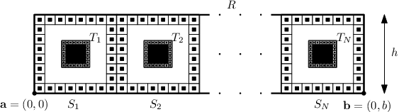
The main idea of the proof is that by choosing $\alpha$ to be very small we force $\varphi$ to map the long edges of the rectangle $R$ to almost straight lines stretched by a factor almost $K$. The function $\rho$ has been constructed so that most of the mass within $S_{i}$ is concentrated on $T_{i}$. This implies that the majority of each $\varphi(S_{i})$ has to be filled up with $\varphi(T_{i})$.

On the other hand, the sidelength of each $T_{i}$ is $\delta$-times smaller than that of $S_{i}$. Each side of $T_{i}$ is also covered with smaller squares, and thus it cannot be stretched more than by the factor $K$. The only way in which all these conditions can be fulfilled is that the images of the long edges of the rectangle $R$ somewhat ripple up above the images of the respective rectangles $T_{i}$, while between them they have to ripple down. But this forces the images of the long edges of $R$ to become very long, eventually longer than the constant $K$ allows, which leads to a contradiction. We illustrate the outlined idea in Figure 3.

In order to make this idea rigorous, we look at the change of the length of vertical cuts through the set $\varphi(R)$. The most complicated part of the proof is an estimation of the length of the boundary of $\varphi(R)$. Because we have almost no control of $\varphi$ locally, the shapes of different $\varphi(S_{i})$ can be various. We manage the described difficulty by examining the squares $S_{i}$ in seven-tuples. For this purpose we make an additional technical assumption that the number of squares covering every edge during the construction of $\rho$ is divisible by seven. Let $R_{i}$ stand for the rectangle formed by the seven consecutive squares $S_{7i-6},\ldots,S_{7i}$. Without loss of generality, we assume that the edges of the squares $S_{i}$ covering the edge $\overline{\mathbf{a}\mathbf{b}}$ are their bottom edges. Let us write $\mathbf{a}_{i}$ and $\mathbf{b}_{i}$ for the left and right vertices at the bottom of the rectangle $R_{i}$, respectively, and $\mathbf{c}_{i}$ and $\mathbf{d}_{i}$ for the left and right vertices on the top of $R_{i}$, respectively.

The factor $1-2\alpha$ in the preceding definition is chosen to have a constant fraction of the rectangles $R_{i}$ nice, more precisely, to get the following observation:

Now, we define the set $D_{i}:=\pi_{x}(\varphi(\overline{\mathbf{a}_{i}\mathbf{b}_{i}}))\cap\pi_{x}(\varphi(\overline{\mathbf{c}_{i}\mathbf{d}_{i}}))$ for every rectangle $R_{i}$. Next, we define a function $f_{i}\colon D_{i}\rightarrow[0,\infty)$ measuring the length of vertical cuts through the set $\varphi(R_{i})$ at a point $x\in D_{i}$, i.e., $f_{i}(x)=\lambda_{1}(\{y\in\mathbb{R}|\,(x,y)\in\varphi(R_{i})\})$. It follows from the continuity of the map $\varphi^{-1}$ that the function $f_{i}$ is Lebesgue integrable for every $R_{i}$.

We would like to stress that the function $f_{i}$ is measuring only the length of cuts through the set $R_{i}$, not the entire $R$. Vertical cuts through $R$ can intersect many $R_{i}$’s.

The following observation will later help us treat each nice rectangle separately. It basically says, that the image of every such an $R_{i}$ is drawn almost horizontally and its boundary is not “too wavy”.

The rectangle $R_{i}$ is formed by the squares $S_{7i-6},\ldots,S_{7i}$. We define the sets $V_{i}:=\pi_{x}(\varphi(T_{7i-3}))$ and $C_{i}:=\pi_{x}(\varphi(S_{7i-3}))\setminus\pi_{x}(\bigcup_{j=7i-6}^{7i}\varphi(T_{j}))$; so we have $V_{i}\cap C_{i}=\emptyset$. By Observation 6 it is clear that $\pi_{x}(\varphi(S_{7i-3}))\subseteq D_{i}$, and thus $C_{i},V_{i}\subseteq D_{i}$ for nice $R_{i}$.

Observation 6 implies that, whenever $R_{i}$ is nice, for every $x\in V_{i}\cup C_{i}$, all the points of intersection of the vertical cut at $x$ with $\partial\varphi(R_{i})$ also lie on $\partial\varphi(R)$. Indeed, since the map $\varphi$ is a homeomorphism, the images of the long edges of $R_{i}$, which form a part of $\partial\varphi(R_{i})$, are also part of $\partial\varphi(R)$. We will use these points to bound the length of the boundary of $\varphi(R)$.

It is possible that the sets $V_{i},V_{i+1},C_{i}$, and $C_{i+1}$ are not mutually disjoint. Let $x$ be a common point of $C_{i}$ and $C_{i+1}$, for example. We already know that, if $R_{i}$ and $R_{i+1}$ are both nice, the points of intersection of $\partial\varphi(R_{i})$ and $\partial\varphi(R_{i+1})$ with the vertical cut at $x$ lie on the boundary of $\varphi(R)$. The fact that $\varphi$ is a homeomorphism implies that all these points are different. This is a crucial observation in our proof, because it allows us to do the estimates for each of the nice rectangles separately and then sum them up.

Let us set $v_{i}:=\lambda_{1}(V_{i})$ and $c_{i}:=\lambda_{1}(C_{i})$. Since the length of the edge of $T_{i}$ is $\delta h$, we have that the length of the boundary of $\varphi(T_{7i-3})$ is at most $4K\delta h$, which implies $\lambda_{1}(\pi_{x}(\varphi(T_{7i-3})))\leq 2K\delta h$, and hence $v_{i}\leq 2K\delta h$ for every $i\in\left\{1,\ldots,N/7\right\}$.

For every nice $R_{i}$ we have $\lambda_{1}(\pi_{x}(\varphi(S_{7i-3})))>K(1-2\alpha)7h-6Kh=Kh(1-14\alpha)$, and thus $c_{i}>Kh(1-14\alpha)-7\cdot 2K\delta h=Kh(1-14\alpha-14\delta)$. Because we need $c_{i}>0$, we have to choose $\delta\in(0,1/14)$ and $\alpha\in(0,(1-14\delta)/14)$.

By Theorem 3 and since we assume $\jac(\varphi)=\rho$ a.e., we have $\lambda(\varphi(T_{7i-3}))=(1-\gamma)h^{2}$. We define two constants $h_{V}^{i}$ and $h_{C}^{i}$ denoting the average values of $f_{i}$ over the sets $V_{i}$ and $C_{i}$, respectively. In other words, the following holds:

The upper bound $v_{i}\leq 2K\delta h$ yields

Using the lower bound $c_{i}>Kh(1-14\alpha-14\delta)$, we deduce that the following holds for every nice $R_{i}$:

Since $h_{V}^{i}$ and $h_{C}^{i}$ are the average values of $f_{i}$ over $V_{i}$ and $C_{i}$, respectively, we get that for every nice $R_{i}$ there must be two points $x_{i}\in V_{i}$ and $y_{i}\in C_{i}$ such that $f_{i}(x_{i})\geq h_{V}^{i}$ and $f_{i}(y_{i})\leq h_{C}^{i}$. Thus we have $f_{i}(x_{i})-f_{i}(y_{i})\geq h_{V}^{i}-h_{C}^{i}$. Furthermore, we can bound the last term using the bounds on $h_{V}^{i}$ and $h_{C}^{i}$ derived above. That is, we infer that $h_{V}^{i}-h_{C}^{i}>\frac{1}{K}\cdot h\cdot\left(\frac{1-\gamma}{2\delta}-\frac{7\gamma}{1-14\alpha-14\delta}\right):=\Delta$. This bound is already independent of $i$. Clearly, $\Delta>0$ if the parameters are chosen appropriately.

Now, we would like to argue that $\Delta$ is the lower bound on the change of height of $\varphi(R)$ over $V_{i}\cup C_{i}$ for every nice $R_{i}$. Indeed, it is true that there are two points $\mathbf{u}_{i},\mathbf{u}^{\prime}_{i}$, the former from the image of the bottom edge $\overline{\mathbf{a}_{i}\mathbf{b}_{i}}$ of $R_{i}$, the latter from the image of the upper edge $\overline{\mathbf{c}_{i}\mathbf{d}_{i}}$, such that $\mathbf{u}_{i}=(x_{i},u_{i})$, $\mathbf{u}^{\prime}_{i}=(x_{i},u^{\prime}_{i})$ and $\left|u^{\prime}_{i}-u_{i}\right|\geq h_{V}^{i}$. But the same thing about $y_{i}$ and $h_{C}^{i}$ has to be said with a little more care.

The problem is that the vertical cut through $\varphi(R_{i})$ at $y_{i}$ does not have to be connected, i.e., it may consist of several line segments even for nice $R_{i}$. But we know that the length of these line segments is at most $h_{C}^{i}$ in total, and hence every line segment of this cut is at most $h_{C}^{i}$ long. Consequently, we infer that there are two points $\mathbf{l}_{i}\in\varphi\left(\overline{\mathbf{a}_{i}\mathbf{b}_{i}}\right),\mathbf{l}^{\prime}_{i}\in\varphi\left(\overline{\mathbf{c}_{i}\mathbf{d}_{i}}\right)$ such that $\mathbf{l}_{i}=(y_{i},l_{i})$, $\mathbf{l}^{\prime}_{i}=(y_{i},l^{\prime}_{i})$ and $\left|l^{\prime}_{i}-l_{i}\right|\leq h_{C}^{i}$. The situation is depicted in Figure 5.

We would like to combine Observation 5 and the discussion above to bound below the vertical distance that has to be overcome by $\varphi(R)$. What we mean by this precisely is explained in the following definition:

In other words, the vertical length of a curve is its length when measuring the distance only in the $y$-coordinate.

Let $J$ be the set of indices $i$ such that $R_{i}$ is nice. By the above discussion, it follows that $\vl(\partial\varphi(R))$ has to be at least $\sum_{i\in J}{\left(\left|u^{\prime}_{i}-l^{\prime}_{i}\right|+\left|u_{i}-l_{i}\right|\right)}$. Next, we bound it below using the triangle and the reverse triangle inequalities:

We have chosen the points $\mathbf{u}^{\prime}_{i},\mathbf{u}_{i},\mathbf{l}^{\prime}_{i}$, and $\mathbf{l}_{i}$ so that, for every nice $R_{i}$, ${\left\|\mathbf{u}^{\prime}_{i}-\mathbf{u}_{i}\right\|_{2}}-{\left\|\mathbf{l}^{\prime}_{i}-\mathbf{l}_{i}\right\|_{2}}>\Delta$. By Observation 5 we know that there are at least $N/14$ nice rectangles $R_{i}$, and thus $\sum_{i\in J}{\left({\left\|\mathbf{u}^{\prime}_{i}-\mathbf{u}_{i}\right\|_{2}}-{\left\|\mathbf{l}^{\prime}_{i}-\mathbf{l}_{i}\right\|_{2}}\right)}$ is at least $\Delta N/14$.

Let $P$ stand for $\left(\partial\varphi(R)\right)\setminus\varphi(\overline{\mathbf{a}\mathbf{b}})$. It is easy to see that

since the points $\mathbf{u}^{\prime}_{i},\mathbf{l}^{\prime}_{i}$ are lying on $P$ in order specified by $i$. Now, we aim to obtain a lower bound on the latter quantity.

Before we proceed, we would like to describe the strategy used in the rest of the proof. We know that the curve $\varphi(\overline{\mathbf{a}\mathbf{b}})$ is at most $Kb$ long and connects the points $\varphi(\mathbf{a})$ and $\varphi(\mathbf{b})$ at distance almost $Kb$. This means that $\vl(\varphi(\overline{\mathbf{a}\mathbf{b}}))$ has to be very small. On the other hand, we have a lower bound on $\vl\left(\partial\varphi(R)\right)$, which implies a lower bound on $\vl(P)$. Moreover, $P$ also connects the points $\varphi(\mathbf{a})$ and $\varphi(\mathbf{b})$; therefore, together with the lower bound on $\vl(P)$, we can calculate a lower bound on $\len(P)$ that becomes large if the parameters are chosen appropriately, eventually larger than the constant $K$ allows. This will be the desired contradiction.

As we already know, the vertical length of the whole boundary of $\varphi(R)$ is at least $\sum_{i\in J}{\left(\left|u^{\prime}_{i}-l^{\prime}_{i}\right|+\left|u_{i}-l_{i}\right|\right)}$, which in turn is at least $\Delta N/14$. Subtracting the second terms of the sum we get the following inequality:

Consequently, in order to get the desired lower bound on $\vl(P)$, it suffices to derive an upper bound on the quantity $\sum_{i\in J}\left|u_{i}-l_{i}\right|$, which in turn is a lower bound on $\vl(\varphi(\overline{\mathbf{a}\mathbf{b}}))$. To this end, we use the following simple geometric considerations.

The curve $\varphi(\overline{\mathbf{a}\mathbf{b}})$ connects the points $\varphi(\mathbf{a})$ and $\varphi(\mathbf{b})$ and has a certain length. If we imagine that this curve becomes an inextensible string pinned to the points $\varphi(\mathbf{a})$ and $\varphi(\mathbf{b})$ in the plane, we can use it to construct an ellipse. We pull the string using a pencil to form a triangle. Then, with a tip of the pencil, while keeping the string taut, we draw an ellipse. This is known as the gardener’s construction. An upper bound on the length of the minor axis of the described ellipse is calculated in the next observation, in which we also show that it upper bounds $\vl(\varphi(\overline{\mathbf{a}\mathbf{b}}))$.

Applying the observation above to $\varphi(\overline{\mathbf{a}\mathbf{b}})$, we infer that $Kb\cdot\sqrt{\alpha(2-\alpha)}>\vl(\varphi(\overline{\mathbf{a}\mathbf{b}}))\geq\sum_{i\in J}\left|u_{i}-l_{i}\right|$.

References

- [BK98] D. Burago and B. Kleiner. Separated nets in Euclidean space and Jacobians of bi-Lipschitz maps. Geometric And Functional Analysis, 8:273–282, 1998.
- [DM90] B. Dacorogna and J. Moser. On a partial differential equation involving the Jacobian determinant. Annales de l’institut Henri Poincaré (C) Analyse non linéaire, 7(1):1–26, 1990.
- [Fre00] D. H. Fremlin. Measure Theory. Number vol. 2: Broad Foundations in Measure Theory. Torres Fremlin, 2000.
- [Gro93] M. L. Gromov. Geometric Group Theory: Asymptotic invariants of infinite groups. London Mathematical Society lecture note series. Cambridge University Press, 1993.
- [Kal12] V. Kaluža. Lipschitz mappings of discrete sets. Bachelor thesis, Faculty of Mathematics and Physics, Charles University in Prague, 2012. [in Czech].
- [McM98] C. T. McMullen. Lipschitz maps and nets in Euclidean space. Geometric And Functional Analysis, 8:304–314, 1998.
- [Ye94] D. Ye. Prescribing the Jacobian determinant in Sobolev spaces. Annales de l’institut Henri Poincaré (C) Analyse non linéaire, 11(3):275–296, 1994.