跳到论文正文
W Papers独立论文阅读器 arXiv:1404.5814 论文正文 计算阅读时间 · 0%
引用这篇论文根据当前论文元数据生成,正式投稿前建议核对。


License: arXiv.org perpetual non-exclusive license
arXiv:1404.5814v1 [math-ph] 23 Apr 2014

Mean exit time for surface-mediated diffusion: spectral analysis and asymptotic behavior

O. Bénichou11 1 Laboratoire de Physique Théorique de la Matière Condensée (UMR 7600), CNRS / UPMC, 4 Place Jussieu, 75255 Paris Cedex    D. S. Grebenkov22 2 Laboratoire de Physique de la Matière Condensée (UMR 7643) CNRS – Ecole Polytechnique, 91128 Palaiseau, France    L. Hillairet33 3 MAPMO (UMR 6628), Université d’Orléans, 45067 Orléans, France    L. Phun33 3 MAPMO (UMR 6628), Université d’Orléans, 45067 Orléans, France    R. Voituriez11 1 Laboratoire de Physique Théorique de la Matière Condensée (UMR 7600), CNRS / UPMC, 4 Place Jussieu, 75255 Paris Cedex    M. Zinsmeister33 3 MAPMO (UMR 6628), Université d’Orléans, 45067 Orléans, France 44 4 Corresponding author: zins@univ-orleans.fr
Abstract

We consider a model of surface-mediated diffusion with alternating phases of pure bulk and surface diffusion. For this process, we compute the mean exit time from a disk through a hole on the circle. We develop a spectral approach to this escape problem in which the mean exit time is explicitly expressed through the eigenvalues of the related self-adjoint operator. This representation is particularly well suited to investigate the asymptotic behavior of the mean exit time in the limit of large desorption rate λ\lambda. For a point-like target, we show that the mean exit time diverges as λ\sqrt{\lambda}. For extended targets, we establish the asymptotic approach to a finite limit. In both cases, the mean exit time is shown to asymptotically increase as λ\lambda tends to infinity. We also revise the optimality regime of surface-mediated diffusion. Although the presentation is limited to the unit disk, the spectral approach can be extended to other domains such as rectangles or spheres.

Received: August 24, 2026/ Revised version:

1 Introduction

Many transport and search processes exhibit intermittent character when different modes of motion are alternated. Typical examples are animals foraging (with phases of rapid relocation and slow exploration), facilitated search mechanism on DNA (with phases of pure bulk diffusion and chain sliding), vesicle transportation in living cells (with phases of active transport by motor proteins and passive diffusion in the cytoplasm), water transport in confining media (with phases of pure bulk diffusion and surface exploration) [3, 4]. The intermittence is often expected to facilitate transport and search processes, e.g., by reducing the mean search time necessary to reach a target (food, specific DNA sequence, nucleus, or reaction zone in the above examples). In particular, the mean exit time from a bounded domain through an opening (a target) on the boundary has been actively studied during the last decade [9, 8]. For pure bulk diffusion, Singer et al. derived the asymptotic behavior of the mean exit time in the narrow escape limit (when the size of the target is small) [21, 19, 20, 18, 10]. Isaacson and Newby developed uniform in time asymptotic expansions in the target radius of the first passage time density for the diffusing molecule to find the target [7]. The escape problem for an intermittent process with phases of surface and pure bulk diffusion (the so-called surface-mediated diffusion) has been recently solved for rotation-invariant domains [1, 2]. The known eigenbases for the Laplace operators governing pure bulk and surface diffusions allowed one to express the mean exit time in a closed matrix form. Under well-defined conditions, the mean exit time was shown to be minimized at an optimal desorption rate that characterizes switching from surface to pure bulk diffusion. These results have been extended in various directions [16, 17, 5, 6]. An alternative master equation approach for discrete (on-lattice) surface-mediate diffusion (also called the bulk-mediated surface diffusion) has been proposed [11, 14, 12, 13].

In the present paper, we propose a rigorous spectral analysis of the above escape problem. We focus on surface-mediated diffusion in the unit disk and derive a spectral representation of the mean exit time. This representation is well suited to investigate the asymptotic behavior of the mean exit time in the limit of large desorption rate λ\lambda. For a point-like target, we show that the mean exit time diverges as λ\sqrt{\lambda}. For extended targets, we establish the asymptotic approach to a finite limit. In both cases, the mean exit time is shown to asymptotically increase as λ\lambda tends to infinity. We also revise the optimality regime of surface-mediated diffusion. Although the presentation is limited to the unit disk, the spectral approach can be extended to other domains such as rectangles or spheres.

2 A self-adjoint operator formulation

We study the following model of surface-mediated diffusion in the unit disk 𝔻={z∈ℂ:|z|<1}\mathbb{D}=\{z\in\mathbb{C}~:|z|<1\} whose boundary ∂𝔻\partial\mathbb{D} includes an exit (or a target) of angular size 2​ϵ2\epsilon (i.e., an arc of the unit circle between π−ϵ\pi-\epsilon and π+ϵ\pi+\epsilon), with 0≤ϵ≤π0\leq\epsilon\leq\pi. A starting point ei​θe^{i\theta} is taken on the unit circle. If the starting point is located on the target then the process is immediately stopped. Otherwise, the particle moves along the circle according to a Brownian motion with the diffusion coefficient D1D_{1} for a duration of min⁡{τλ,τ}\min\{\tau_{\lambda},\tau\}, where τλ\tau_{\lambda} is a random variable with exponential law of parameter λ≥0\lambda\geq 0, and τ\tau is the first hitting time of the target. If τ≤τλ\tau\leq\tau_{\lambda} then the process stops. If τ>τλ\tau>\tau_{\lambda} then the particle is relocated at time τλ\tau_{\lambda} along the normal inside the disk at a distance 0<a≤10<a\leq 1 to start there a 2D Brownian motion with the diffusion coefficient D2D_{2}. This motion is stopped after hitting back the unit circle, and the same procedure is restarted from this last hitting point. We define t1​(θ)t_{1}(\theta) as being the expected time to reach the target. Similarly, for 0≤r<10\leq r<1, we define t2​(r​ei​θ)t_{2}(re^{i\theta}) as being the expected time to reach the target starting from the point r​ei​θre^{i\theta} inside the unit disk.

It has been shown in [2] that these two functions satisfy the following system of equations:

D1​t1′′​(θ)+λ⁡[t2​((1−a)​ei​θ)−t1​(θ)]=−1\displaystyle D_{1}t_{1}^{\prime\prime}(\theta)+\lambda[t_{2}\left((1-a)e^{i\theta}\right)-t_{1}(\theta)]=-1 (1)
D2​Δ​t2=−1\displaystyle D_{2}\Delta t_{2}=-1 (2)
t2(ei​θ)=t1(θ) (θ∈[−π,π])\displaystyle t_{2}(e^{i\theta})=t_{1}(\theta)\text{ }(\theta\in[-\pi,\pi]) (3)
t1​(θ)=0​ if ​θ∈[−π,−π+ϵ]∪[π−ϵ,π]\displaystyle t_{1}(\theta)=0\text{ if }\theta\in[-\pi,-\pi+\epsilon]\cup[\pi-\epsilon,\pi] (4)

Let us notice that, by symmetry, t1​(θ)t_{1}(\theta) is an even function so it is sufficient to determine it on [0,π][0,\pi].

The solution to Eq. (2) is the sum of the particular solution 1−r24​D2\frac{1-r^{2}}{4D_{2}} to the inhomogeneous (Poisson) equation Δ​u=−1D2,u|∂𝔻=0\Delta u=-\frac{1}{D_{2}},~u|_{\partial\mathbb{D}}=0, and the solution to the Dirichlet problem Δ​v=0\Delta v=0, v|∂𝔻=t1v|_{\partial\mathbb{D}}=t_{1}.

Since t1t_{1} is even it may be represented as a cosine series

t1​(θ)=∑n≥0an​cos⁡n​θ,t_{1}(\theta)=\sum_{n\geq 0}{a_{n}\cos n\theta},

from which

t2​(r​ei​θ)=1−r24​D2+∑n≥0an​rn​cos⁡n​θ.\displaystyle t_{2}(re^{i\theta})=\frac{1-r^{2}}{4D_{2}}+\sum_{n\geq 0}{a_{n}r^{n}\cos n\theta}.

Eq. (1) then becomes

t1′′​(θ)=−1D1​(1+λ​1−(1−a)24​D2)+λD1​U​(t1),\displaystyle t_{1}^{\prime\prime}(\theta)=-\frac{1}{D_{1}}\left(1+\lambda\frac{1-(1-a)^{2}}{4D_{2}}\right)+\frac{\lambda}{D_{1}}U(t_{1}), (5)

where UU is the operator on L2​([0,π])L^{2}\left([0,\pi]\right) defined by

U⁡(∑n≥0xn​cos⁡n​θ)=∑n≥1xn​(1−(1−a)n)​cos⁡n​θ.\displaystyle U\left(\sum_{n\geq 0}{x_{n}\cos n\theta}\right)=\sum_{n\geq 1}{x_{n}\left(1-(1-a)^{n}\right)\cos n\theta}.

This operator can also be written as U=V2U=V^{2}, where

V⁡(∑n≥0xn​cos⁡n​θ)=∑n≥1xn​1−(1−a)n​cos⁡n​θ.\displaystyle V\left(\sum_{n\geq 0}{x_{n}\cos n\theta}\right)=\sum_{n\geq 1}{x_{n}\sqrt{1-(1-a)^{n}}\cos n\theta}. (6)

Next we introduce the Sturm Liouville operator TT defined on L2​([0,π−ϵ])L^{2}\left([0,\pi-\epsilon]\right) as T​f=uTf=u, where

u′′=f\displaystyle u^{\prime\prime}=f (7)
u′​(0)=u⁡(π−ϵ)=0.\displaystyle u^{\prime}(0)=u(\pi-\epsilon)=0. (8)

The operator TT is negative self-adjoint. Finally, we define T~=−E​T​R\tilde{T}=-ETR as an operator on L2​([0,π])L^{2}\left([0,\pi]\right), where R:L2​([0,π])⟶L2​([0,π−ϵ])R:L^{2}\left([0,\pi]\right)\longrightarrow L^{2}\left([0,\pi-\epsilon]\right) is the natural restriction, and E:L2​([0,π−ϵ])⟶L2​([0,π])E:L^{2}\left([0,\pi-\epsilon]\right)\longrightarrow L^{2}\left([0,\pi]\right) is the natural extension by 00. The operator T~\tilde{T} can be written explicitly as

T~​(f)={∫θπ−ϵd​θ1​∫0θ1d​θ2​f​(θ2),0≤θ<π−ϵ,0,π−ϵ≤θ≤π.\tilde{T}(f)=\begin{cases}\int\limits_{\theta}^{\pi-\epsilon}d\theta_{1}\int\limits_{0}^{\theta_{1}}d\theta_{2}~f(\theta_{2}),\quad 0\leq\theta<\pi-\epsilon,\cr 0,\hskip 88.20354pt\pi-\epsilon\leq\theta\leq\pi.\end{cases} (9)

One can easily check that the eigenbasis of this operator is

νn=(1−ϵ/π)2(n+1/2)2,un={2π−ϵ​cos⁡((n+1/2)​θ1−ϵ/π),0≤θ≤π−ϵ,0,π−ϵ≤θ≤π.\nu_{n}=\frac{(1-\epsilon/\pi)^{2}}{(n+1/2)^{2}},\qquad u_{n}=\begin{cases}\sqrt{\frac{2}{\pi-\epsilon}}\cos\left(\frac{(n+1/2)\theta}{1-\epsilon/\pi}\right),\quad 0\leq\theta\leq\pi-\epsilon,\cr 0,\hskip 99.58464pt\pi-\epsilon\leq\theta\leq\pi.\end{cases} (10)

These eigenvectors form an orthogonal basis of L2​[0,π−ϵ]L^{2}[0,\pi-\epsilon] by Sturm-Liouville theory.

Let us check that T~\tilde{T} is a self-adjoint non-negative operator on L2​([0,π])L^{2}\left([0,\pi]\right). Let ff, gg be in L2​([0,π])L^{2}\left([0,\pi]\right):

−⟨T~​f,g¯⟩\displaystyle-\langle\tilde{T}f,\overline{g}\rangle =⟨E​T​R​f,g¯⟩=∫0π−ϵT⁡(R​f)​g¯=∫0π−ϵT⁡(R​f)​R​g¯\displaystyle=\langle ETRf,\overline{g}\rangle=\int_{0}^{\pi-\epsilon}T(Rf)~\overline{g}=\int_{0}^{\pi-\epsilon}T(Rf)~\overline{Rg}
=∫0π−ϵR​f​T⁡(R​g)¯=∫0πf​E​T​R​(g)¯=−⟨f,T~​g¯⟩,\displaystyle=\int_{0}^{\pi-\epsilon}Rf~\overline{T(Rg)}=\int_{0}^{\pi}f~\overline{ETR(g)}=-\langle f,\overline{\tilde{T}g}\rangle,

which proves the claim, since the operator E​T​RETR is negative.

The operator T~\tilde{T} allows us to translate Eq. (5) into

t1=1D1​(1+λ​1−(1−a)24​D2)​T~​(1)−λD1​T~​U​(t1).\displaystyle t_{1}=\frac{1}{D_{1}}\left(1+\lambda\frac{1-(1-a)^{2}}{4D_{2}}\right)\tilde{T}(1)-\frac{\lambda}{D_{1}}\tilde{T}U(t_{1}). (11)

We next apply the operator VV to both sides of Eq. (11) to get, writing s1=V⁡(t1)s_{1}=V(t_{1}),

s1=1D1​(1+λ​1−(1−a)24​D2)​V​T~​(1)−λD1​V​T~​V​(s1),\displaystyle s_{1}=\frac{1}{D_{1}}\left(1+\lambda\frac{1-(1-a)^{2}}{4D_{2}}\right)V\tilde{T}(1)-\frac{\lambda}{D_{1}}V\tilde{T}V(s_{1}),

which can be solved in s1s_{1} as

s1=1D1​(1+λ​1−(1−a)24​D2)​(I+λD1​V​T~​V)−1​(ψ),\displaystyle s_{1}=\frac{1}{D_{1}}\left(1+\lambda\frac{1-(1-a)^{2}}{4D_{2}}\right)\left(I+\frac{\lambda}{D_{1}}V\tilde{T}V\right)^{-1}(\psi), (12)

where ψ=V​T~​(1)\psi=V\tilde{T}(1). This is an exact solution of the original problem for a fixed starting point. We emphasize that the operators VV and T~\tilde{T}, as well as the function ψ=V​T~​(1)\psi=V\tilde{T}(1), are given explicitly. At first thought, this representation looks similar to the mean exit time found in [2] (see also [16, 17]). Although both derivations are conceptually similar, the major advantage of the present approach is the use of the self-adjoint operator V​T~​VV\tilde{T}V. This feature allows one to invert the operator (I+λD1​V​T~​V)(I+\frac{\lambda}{D_{1}}V\tilde{T}V) in Eq. (14) and to express the mean exit time in a spectral form (see below).

The case of a randomly distributed starting point on the circle with uniform law is of particular interest. This is equivalent to averaging the mean exit time over the starting points that we denote as

⟨t1⟩=1π​∫0πd​θ​t1​(θ)=1π​⟨t1,1⟩.\displaystyle\langle t_{1}\rangle=\frac{1}{\pi}\int_{0}^{\pi}d\theta~t_{1}(\theta)=\frac{1}{\pi}\langle t_{1},1\rangle.

Using Eqs. (11) and (12), we can write

π​⟨t1⟩\displaystyle\pi\langle t_{1}\rangle =1D1​(1+λ​1−(1−a)24​D2)​⟨T~​(1),1⟩−λD1​⟨T~​V​(s1),1⟩\displaystyle=\frac{1}{D_{1}}\left(1+\lambda\frac{1-(1-a)^{2}}{4D_{2}}\right)\langle\tilde{T}(1),1\rangle-\frac{\lambda}{D_{1}}\langle\tilde{T}V(s_{1}),1\rangle
=1D1​(1+λ​1−(1−a)24​D2)​⟨T~​(1),1⟩−λD1​⟨s1,ψ⟩,\displaystyle=\frac{1}{D_{1}}\left(1+\lambda\frac{1-(1-a)^{2}}{4D_{2}}\right)\langle\tilde{T}(1),1\rangle-\frac{\lambda}{D_{1}}\langle s_{1},\psi\rangle, (13)

from which it follows that the knowledge of s1s_{1} allows to compute ⟨t1⟩\langle t_{1}\rangle:

⟨t1⟩\displaystyle\langle t_{1}\rangle =1π​D1​(1+λ​1−(1−a)24​D2)​(⟨T~​(1),1⟩−λD1​⟨(I+λD1​V​T~​V)−1​ψ,ψ⟩).\displaystyle=\frac{1}{\pi D_{1}}\left(1+\lambda\frac{1-(1-a)^{2}}{4D_{2}}\right)\left(\langle\tilde{T}(1),1\rangle-\frac{\lambda}{D_{1}}\langle\left(I+\frac{\lambda}{D_{1}}V\tilde{T}V\right)^{-1}\psi,\psi\rangle\right). (14)

By spectral theorem there exists an orthonormal basis of L2​([0,π])L^{2}\left([0,\pi]\right) which diagonalizes the self-adjoint operator V​T~​VV\tilde{T}V. More precisely, L2​([0,π])L^{2}\left([0,\pi]\right) is the orthogonal direct sum of ker⁡(V​T~​V)\ker(V\tilde{T}V) and Im⁡(V​T~​V)\Ima(V\tilde{T}V) and we obtain this orthonormal basis by completing any orthonormal basis of ker⁡(V​T~​V)\ker(V\tilde{T}V) with the basis formed by the normalized eigenvectors associated with positive eigenvalues.

To identify these two spaces let us notice first that ker⁡V\ker V is the one dimensional space of constant functions. Thus ker⁡(V​T~​V)\ker(V\tilde{T}V) is the space of functions f∈L2​([0,π])f\in L^{2}\left([0,\pi]\right) such that T~​(V​f)\tilde{T}(Vf) is constant. But since V​f=T~​(V​f)′′Vf=\tilde{T}(Vf)^{\prime\prime} on [0,π−ϵ][0,\pi-\epsilon], V​f≡0Vf\equiv 0 on [0,π−ϵ][0,\pi-\epsilon]. So f∈ker⁡(V​T~​V)⇒supp(V​f)⊂[π−ϵ,π]f\in\ker(V\tilde{T}V)\Rightarrow\mathop{\operator@font supp}\nolimits(Vf)\subset[\pi-\epsilon,\pi], and this implication is easily seen to be an equivalence. With a slight abuse of language, we write ker⁡(V​T~​V)=V−1​(L2​(π−ϵ,π))\ker(V\tilde{T}V)=V^{-1}\left(L^{2}\left(\pi-\epsilon,\pi\right)\right). It follows that Im⁡(V​T~​V)=V⁡(L2​([0,π−ϵ]))\Ima(V\tilde{T}V)=V\left(L^{2}\left([0,\pi-\epsilon]\right)\right).

We call (en)n≥0\left(e_{n}\right)_{n\geq 0} the orthonormal basis of Im⁡(V​T~​V)\Ima(V\tilde{T}V) such that V​T~​V​en=λn​enV\tilde{T}Ve_{n}=\lambda_{n}e_{n} and λn↓0\lambda_{n}\downarrow 0 as n→∞n\to\infty.

When ϵ=0\epsilon=0, the eigenbasis ene_{n} is simply formed by cosine functions, and the analysis is straightforward (see below). When ϵ>0\epsilon>0, we first observe that ψ=V​T~​(1)=V​T~​(φ0)\psi=V\tilde{T}(1)=V\tilde{T}(\varphi_{0}) where

φ0={1 on [0,π−ϵ[,−π−ϵϵ on ​[π−ϵ,π].\displaystyle\varphi_{0}=\begin{cases}1&\text{ on }[0,\pi-\epsilon[,\\ -\frac{\pi-\epsilon}{\epsilon}&\text{ on }[\pi-\epsilon,\pi].\end{cases}

so that ∫0πφ0=0\int_{0}^{\pi}{\varphi_{0}}=0, and thus there exists ψ0∈L2​([0,π])\psi_{0}\in L^{2}\left([0,\pi]\right) such that φ0=V​ψ0\varphi_{0}=V\psi_{0}. It follows that ψ∈Im⁡(V​T~​V)\psi\in\Ima(V\tilde{T}V) and we can write

ψ=∑n≥1ψn​en,\displaystyle\psi=\sum_{n\geq 1}{\psi_{n}e_{n}},

with coefficients ψn\psi_{n} forming a sequence in ℓ2\ell^{2}. Using this representation, Eq. (12) is formally solved as

s1=1D1​(1+λ​1−(1−a)24​D2)​∑n≥1ψn1+λD1​λn​en.\displaystyle s_{1}=\frac{1}{D_{1}}\left(1+\lambda\frac{1-(1-a)^{2}}{4D_{2}}\right)\sum_{n\geq 1}{\frac{\psi_{n}}{1+\frac{\lambda}{D_{1}}\lambda_{n}}~e_{n}}.

Plugging this expression into Eq. (14) we obtain

⟨t1⟩=1π​D1​(1+λ​1−(1−a)24​D2)​[⟨T~​(1),1⟩−λD1​∑n≥0ψn21+λD1​λn].\displaystyle\langle t_{1}\rangle=\frac{1}{\pi D_{1}}\left(1+\lambda\frac{1-(1-a)^{2}}{4D_{2}}\right)\left[\langle\tilde{T}(1),1\rangle-\frac{\lambda}{D_{1}}\sum_{n\geq 0}{\frac{\psi_{n}^{2}}{1+\frac{\lambda}{D_{1}}\lambda_{n}}}\right]. (15)

This spectral representation is particularly well suited for the asymptotic analysis of the mean exit time.

2.1 Point-like target (ϵ=0\epsilon=0)

We first consider the case of ϵ=0\epsilon=0. Although such a target is not accessible for 2D pure bulk diffusion, it can still be reached through 1D surface diffusion. In this case, one easily gets

{T~​(cos⁡n​θ)=−T⁡(cos⁡n​θ)=cos⁡n​θ−(−1)nn2(n≥1),T~​(1)=−T​(1)=π2−θ22,\displaystyle\begin{cases}\tilde{T}(\cos n\theta)=-T(\cos n\theta)=\frac{\cos n\theta-(-1)^{n}}{n^{2}}\quad(n\geq 1),\\ \tilde{T}(1)=-T(1)=\frac{\pi^{2}-\theta^{2}}{2},\end{cases} (16)

so that

{V​T~​V​(cos⁡n​θ)=1−(1−a)nn2​cos⁡n​θ(n≥1),V​T~​V​(1)=0.\displaystyle\begin{cases}V\tilde{T}V(\cos n\theta)=\frac{1-(1-a)^{n}}{n^{2}}\cos n\theta\quad(n\geq 1),\\ V\tilde{T}V(1)=0.\end{cases} (17)

One concludes that

λn={1−(1−a)nn2(n≥1),0(n=0),en={2/π​cos⁡n​θ(n≥1),1/π(n=0).\lambda_{n}=\begin{cases}\frac{1-(1-a)^{n}}{n^{2}}\quad(n\geq 1),\cr 0\hskip 42.67912pt(n=0),\end{cases}\qquad e_{n}=\begin{cases}\sqrt{2/\pi}\cos n\theta\quad(n\geq 1),\cr\sqrt{1/\pi}\hskip 39.83385pt(n=0).\end{cases} (18)

For n≥1n\geq 1, we have

ψn\displaystyle\psi_{n} =⟨ψ,en⟩=⟨V​T~​(1),en⟩=2/π​⟨T~​(1),V⁡(cos⁡n​θ)⟩\displaystyle=\langle\psi,e_{n}\rangle=\langle V\tilde{T}(1),e_{n}\rangle=\sqrt{2/\pi}~\langle\tilde{T}(1),V(\cos n\theta)\rangle
=2/π​1−(1−a)n​⟨π2−θ22,cos⁡n​θ⟩=2​π​1−(1−a)n​(−1)n+1n2,\displaystyle=\sqrt{2/\pi}\sqrt{1-(1-a)^{n}}~\langle\frac{\pi^{2}-\theta^{2}}{2},\cos n\theta\rangle=\sqrt{2\pi}\sqrt{1-(1-a)^{n}}~\frac{(-1)^{n+1}}{n^{2}}, (19)

while ⟨ψ,1⟩=⟨V​T~​(1),1⟩=⟨T~​(1),V​1⟩=0\langle\psi,1\rangle=\langle V\tilde{T}(1),1\rangle=\langle\tilde{T}(1),V1\rangle=0. Substituting this expression into Eq. (15), we get

⟨t1⟩ϵ=0\displaystyle\langle t_{1}\rangle_{\epsilon=0} =1π​D1​(1+λ​1−(1−a)24​D2)​(⟨T~​(1),1⟩−∑n≥12​π​λD1​(1−(1−a)n)n2​(n2+λD1​(1−(1−a)n)))\displaystyle=\frac{1}{\pi D_{1}}\left(1+\lambda\frac{1-(1-a)^{2}}{4D_{2}}\right)\left(\langle\tilde{T}(1),1\rangle-\sum_{n\geq 1}{\frac{2\pi\frac{\lambda}{D_{1}}\left(1-(1-a)^{n}\right)}{n^{2}\left(n^{2}+\frac{\lambda}{D_{1}}\left(1-(1-a)^{n}\right)\right)}}\right)
=1π​D1​(1+λ​1−(1−a)24​D2)​(⟨T~​(1),1⟩−2​π​∑n≥11n2CLOSE\displaystyle=\frac{1}{\pi D_{1}}\left(1+\lambda\frac{1-(1-a)^{2}}{4D_{2}}\right)\Biggl(\langle\tilde{T}(1),1\rangle-2\pi\sum_{n\geq 1}{\frac{1}{n^{2}}}
+2π∑n≥11n2+λD1​(1−(1−a)n)).\displaystyle+2\pi\sum_{n\geq 1}{\frac{1}{n^{2}+\frac{\lambda}{D_{1}}\left(1-(1-a)^{n}\right)}}\Biggr). (20)

From Eq. (16), we get

⟨T~​(1),1⟩ϵ=0=∫0πd​θ​π2−θ22=13​π3.\displaystyle\langle\tilde{T}(1),1\rangle_{\epsilon=0}=\int\limits_{0}^{\pi}d\theta~\frac{\pi^{2}-\theta^{2}}{2}=\frac{1}{3}\pi^{3}. (21)

We also know the value of the Riemann zeta function

ζ⁡(2)=∑n≥11n2=π26.\displaystyle\zeta(2)=\sum_{n\geq 1}{\frac{1}{n^{2}}}=\frac{\pi^{2}}{6}. (22)

Plugging Eqs. (21) and (22) into Eq. (20) yields

⟨t1⟩ϵ=0\displaystyle\langle t_{1}\rangle_{\epsilon=0} =2D1​(1+λ​1−(1−a)24​D2)​∑n≥11n2+λD1​(1−(1−a)n).\displaystyle=\frac{2}{D_{1}}\left(1+\lambda\frac{1-(1-a)^{2}}{4D_{2}}\right)\sum_{n\geq 1}{\frac{1}{n^{2}+\frac{\lambda}{D_{1}}\left(1-(1-a)^{n}\right)}}. (23)

We retrieved the exact representation of the mean exit time for point-like target that was first derived in [1].

For 0<a<10<a<1, in the following inequalities

∑n≥11n2+λD1\displaystyle\sum_{n\geq 1}{\frac{1}{n^{2}+\frac{\lambda}{D_{1}}}} ≤∑n≥11n2+(1−(1−a)n)​λD1≤∑n≥11n2+a​λD1,\displaystyle\leq\sum_{n\geq 1}{\frac{1}{n^{2}+(1-(1-a)^{n})\frac{\lambda}{D_{1}}}}\leq\sum_{n\geq 1}{\frac{1}{n^{2}+a\frac{\lambda}{D_{1}}}},

Since f⁡(x)=1x2+a​λD1f(x)=\frac{1}{x^{2}+\frac{a\lambda}{D_{1}}} is decreasing, by applying the property that ∫nn+1f⁡(x)​𝑑x≤f⁡(n)≤∫n−1nf⁡(x)​𝑑x\int_{n}^{n+1}{f(x)dx}\leq f(n)\leq\int_{n-1}^{n}{f(x)dx}, one can replace sums by integrals to get

D1λ​π2​F​(D1/λ)\displaystyle\sqrt{\frac{D_{1}}{\lambda}}\frac{\pi}{2}F(D_{1}/\lambda) ≤∑n≥11n2+(1−(1−a)n)​λD1≤D1a​λ​π2,\displaystyle\leq\sum_{n\geq 1}{\frac{1}{n^{2}+(1-(1-a)^{n})\frac{\lambda}{D_{1}}}}\leq\sqrt{\frac{D_{1}}{a\lambda}}\frac{\pi}{2},

where F⁡(x)=1−2π​arctan⁡(x)F(x)=1-\frac{2}{\pi}\arctan(\sqrt{x}). One obtains therefore

π​F​(D1/λ)D1​λ​(1+λ​1−(1−a)24​D2)\displaystyle\frac{\pi F(D_{1}/\lambda)}{\sqrt{D_{1}\lambda}}\left(1+\lambda\frac{1-(1-a)^{2}}{4D_{2}}\right) ≤⟨t1⟩ϵ=0≤πa​D1​λ​(1+λ​1−(1−a)24​D2).\displaystyle\leq\langle t_{1}\rangle_{\epsilon=0}\leq\frac{\pi}{\sqrt{aD_{1}\lambda}}\left(1+\lambda\frac{1-(1-a)^{2}}{4D_{2}}\right). (24)

In the limit of large λ\lambda, F⁡(x)F(x) can be approximated by 11, i.e.

1−(1−a)24​D2​D1​π​λ+πD1​λ\displaystyle\frac{1-(1-a)^{2}}{4D_{2}\sqrt{D_{1}}}\pi\sqrt{\lambda}+\frac{\pi}{\sqrt{D_{1}\lambda}} ≲⟨t1⟩ϵ=0≤1−(1−a)24​D2​D1​a​π​λ+πD1​a​λ.\displaystyle\lesssim\langle t_{1}\rangle_{\epsilon=0}\leq\frac{1-(1-a)^{2}}{4D_{2}\sqrt{D_{1}a}}\pi\sqrt{\lambda}+\frac{\pi}{\sqrt{D_{1}a\lambda}}. (25)

Therefore, we conclude that ⟨t1⟩ϵ=0\langle t_{1}\rangle_{\epsilon=0} asymptotically increases to infinity, as illustrated on Fig. 1a. As a result, if ∂⟨t1⟩ϵ=0∂λ|λ=0<0\left.\frac{\partial\langle t_{1}\rangle_{\epsilon=0}}{\partial\lambda}\right|_{\lambda=0}<0, then ⟨t1⟩ϵ=0\langle t_{1}\rangle_{\epsilon=0} has a minimum. We compute

∂⟨t1⟩ϵ=0∂λ|λ=0=2D1​(1−(1−a)24​D2​∑n≥11n2−1D1​∑n≥11−(1−a)nn4)<0\displaystyle\left.\frac{\partial\langle t_{1}\rangle_{\epsilon=0}}{\partial\lambda}\right|_{\lambda=0}=\frac{2}{D_{1}}\left(\frac{1-(1-a)^{2}}{4D_{2}}\sum_{n\geq 1}{\frac{1}{n^{2}}}-\frac{1}{D_{1}}\sum_{n\geq 1}{\frac{1-(1-a)^{n}}{n^{4}}}\right)<0
⇔1−(1−a)24​D2​π26<1D1​∑n≥11−(1−a)nn4\displaystyle\Leftrightarrow\frac{1-(1-a)^{2}}{4D_{2}}\frac{\pi^{2}}{6}<\frac{1}{D_{1}}\sum_{n\geq 1}{\frac{1-(1-a)^{n}}{n^{4}}}
⇔D2>D2,crit=D1​π2​(1−(1−a)2)24​∑n≥11−(1−a)nn4\displaystyle\Leftrightarrow D_{2}>D_{2,\rm crit}=D_{1}\frac{\pi^{2}(1-(1-a)^{2})}{24\sum_{n\geq 1}{\frac{1-(1-a)^{n}}{n^{4}}}} (26)

We retrieved the optimality condition first reported in [1]. The relation (26) determines the critical value of the pure bulk diffusion coefficient D2,critD_{2,\rm crit}, which for small aa can be approximated as

lima→0D2,crit=D1​π212​ζ​(3)≈0.68​D1.\lim_{a\rightarrow 0}D_{2,\rm crit}=D_{1}\frac{\pi^{2}}{12\zeta(3)}\approx 0.68D_{1}. (27)

If D2>D2,critD_{2}>D_{2,\rm crit}, then ⟨t1⟩ϵ=0\langle t_{1}\rangle_{\epsilon=0} has a minimum.

Refer to caption
Refer to caption
Fig. 1: Mean exit time ⟨t1⟩\langle t_{1}\rangle as a function of λ\lambda for ϵ=0\epsilon=0 (a) and ϵ=0.01\epsilon=0.01 (b), with a=0.01a=0.01 and D1=1D_{1}=1. When D2=0.5<D2,critD_{2}=0.5<D_{2,\rm crit} (blue solid line), ⟨t1⟩\langle t_{1}\rangle monotonously increases with λ\lambda so that the smallest mean exit time corresponds to λ=0\lambda=0 (surface diffusion without intermittence). When D2=2>D2,critD_{2}=2>D_{2,\rm crit} (red dashed line), ⟨t1⟩\langle t_{1}\rangle starts first to decrease with λ\lambda, passes through a minimum and monotonously increases to infinity. For point-like target (a), thin solid lines indicate the leading term of the lower bound 1−(1−a)24​D2​D1​π​λ\frac{1-(1-a)^{2}}{4D_{2}\sqrt{D_{1}}}\pi\sqrt{\lambda} from Eq. (25). Note that the upper bound, which is larger by a−1/2a^{-1/2}, strongly overestimates the mean exit time. Finally, correction terms of the order λ−1/2\lambda^{-1/2} are negligible for large λ\lambda. For extended target (b), horizontal lines indicate the limiting values of the mean exit time as λ→∞\lambda\to\infty. Symbols present the diagonal approximation (46).

2.2 Extended target (ϵ>0\epsilon>0)

In sharp contrast to a point-like target, the mean exit time ⟨t1⟩\langle t_{1}\rangle to an extended target (ϵ>0\epsilon>0) converges in a finite limit as λ→∞\lambda\rightarrow\infty. As a consequence, the quantity ⟨T~​(1),1⟩−λD1​∑n≥0ψn21+λD1​λn\langle\tilde{T}(1),1\rangle-\frac{\lambda}{D_{1}}\sum_{n\geq 0}{\frac{\psi_{n}^{2}}{1+\frac{\lambda}{D_{1}}\lambda_{n}}} must converge to 00 as λ→∞\lambda\rightarrow\infty. Given that

limλ→∞∑n≥1λ​ψn21+λD1​λn=D1​∑n≥1ψn2λn,\displaystyle\lim_{\lambda\rightarrow\infty}{\sum_{n\geq 1}{\frac{\lambda\psi_{n}^{2}}{1+\frac{\lambda}{D_{1}}\lambda_{n}}}}=D_{1}\sum_{n\geq 1}{\frac{\psi_{n}^{2}}{\lambda_{n}}},

we deduce

⟨T~​(1),1⟩=∑n≥1ψn2λn,\displaystyle\langle\tilde{T}(1),1\rangle=\sum_{n\geq 1}{\frac{\psi_{n}^{2}}{\lambda_{n}}}, (28)

and this series converges. Setting λ=0\lambda=0 into Eq. (15), the above expression can be identified to the mean exit time for surface diffusion phase:

⟨t1⟩λ=0=1π​D1​∑n≥1ψn2λn=1π​D1​⟨T~​(1),1⟩=(π−ϵ)33​π​D1,\langle t_{1}\rangle_{\lambda=0}=\frac{1}{\pi D_{1}}\sum_{n\geq 1}{\frac{\psi_{n}^{2}}{\lambda_{n}}}=\frac{1}{\pi D_{1}}\langle\tilde{T}(1),1\rangle=\frac{(\pi-\epsilon)^{3}}{3\pi D_{1}}, (29)

because T~​(1)=(π−ϵ)2−θ22\tilde{T}(1)=\frac{(\pi-\epsilon)^{2}-\theta^{2}}{2} for 0≤θ<π−ϵ0\leq\theta<\pi-\epsilon, and 00 otherwise.

Plugging Eq. (28) into Eq. (15), we obtain

⟨t1⟩=1π​(1λ+1−(1−a)24​D2)​∑n≥1ψn2λn​(D1λ+λn).\displaystyle\langle t_{1}\rangle=\frac{1}{\pi}\left(\frac{1}{\lambda}+\frac{1-(1-a)^{2}}{4D_{2}}\right)\sum_{n\geq 1}\frac{\psi_{n}^{2}}{\lambda_{n}\left(\frac{D_{1}}{\lambda}+\lambda_{n}\right)}. (30)

This formula generalizes Eq. (23) to extended targets.

Similarly, we have

limλ→∞∑n≥1ψn2λn​(D1λ+λn)=∑n≥1ψn2λn2,\displaystyle\lim_{\lambda\rightarrow\infty}{\sum_{n\geq 1}{\frac{\psi_{n}^{2}}{\lambda_{n}\left(\frac{D_{1}}{\lambda}+\lambda_{n}\right)}}}=\sum_{n\geq 1}{\frac{\psi_{n}^{2}}{\lambda_{n}^{2}}},

so that

𝒯=limλ→∞⟨t1⟩=1−(1−a)24​π​D2​∑n≥1ψn2λn2,\displaystyle{\mathcal{T}}=\lim_{\lambda\rightarrow\infty}{\langle t_{1}\rangle}=\frac{1-(1-a)^{2}}{4\pi D_{2}}\sum_{n\geq 1}{\frac{\psi_{n}^{2}}{\lambda_{n}^{2}}}, (31)

i.e., we got a spectral representation for the time 𝒯{\mathcal{T}} corresponding to pure bulk diffusion. Note also that the series S=∑n≥1ψn2λn2S=\sum_{n\geq 1}{\frac{\psi_{n}^{2}}{\lambda_{n}^{2}}} converges.

We may now state the main theorem of this work:

Theorem 1.

The function λ↦⟨t1⟩\lambda\mapsto\langle t_{1}\rangle is eventually increasing as λ→+∞\lambda\rightarrow+\infty. Moreover, if

d​⟨t1⟩d​λ|λ=0<0,\displaystyle\left.\frac{d\langle t_{1}\rangle}{d\lambda}\right|_{\lambda=0}<0,

then the function ⟨t1⟩\langle t_{1}\rangle passes through a minimum.

Proof.
Lemma 2.
∑n≥1ψn2λn3=+∞.\displaystyle\sum_{n\geq 1}{\frac{\psi_{n}^{2}}{\lambda_{n}^{3}}}=+\infty.

The proof of this lemma will be given in the next section. We assume it is true for the rest of the proof of the main theorem.

We rewrite Eq. (30) as follows

⟨t1⟩=𝒯+Sπ​λ−D1λ​1−(1−a)24​π​D2​∑n≥1ψn2λn2​(λn+D1λ)−D1π​λ2​∑n≥1ψn2λ2​(λn+D1λ).\displaystyle\langle t_{1}\rangle={\mathcal{T}}+\frac{S}{\pi\lambda}-\frac{D_{1}}{\lambda}\frac{1-(1-a)^{2}}{4\pi D_{2}}\sum_{n\geq 1}{\frac{\psi_{n}^{2}}{\lambda_{n}^{2}\left(\lambda_{n}+\frac{D_{1}}{\lambda}\right)}}-\frac{D_{1}}{\pi\lambda^{2}}\sum_{n\geq 1}{\frac{\psi_{n}^{2}}{\lambda^{2}\left(\lambda_{n}+\frac{D_{1}}{\lambda}\right)}}. (32)

Since

limλ→∞∑n≥1ψn2λn2​(λn+D1λ)=∑n≥1ψn2λn3=+∞,\displaystyle\lim_{\lambda\rightarrow\infty}{\sum_{n\geq 1}{\frac{\psi_{n}^{2}}{\lambda_{n}^{2}\left(\lambda_{n}+\frac{D_{1}}{\lambda}\right)}}}=\sum_{n\geq 1}{\frac{\psi_{n}^{2}}{\lambda_{n}^{3}}}=+\infty,

we see that

⟨t1⟩=𝒯−D1λ​1−(1−a)24​π​D2​∑n≥1ψn2λn2​(λn+D1λ)+O⁡(λ−1),\displaystyle\langle t_{1}\rangle={\mathcal{T}}-\frac{D_{1}}{\lambda}\frac{1-(1-a)^{2}}{4\pi D_{2}}\sum_{n\geq 1}{\frac{\psi_{n}^{2}}{\lambda_{n}^{2}\left(\lambda_{n}+\frac{D_{1}}{\lambda}\right)}}+O(\lambda^{-1}),

from which the principle part of ⟨t1⟩\langle t_{1}\rangle is indeed non-decreasing as λ→∞\lambda\rightarrow\infty.

To complete the proof, we differentiate Eq. (32) (the exchange of derivative and sum is easily established):

π​d​⟨t1⟩d​λ=−Sλ2+1λ2​D1​(1−(1−a)2)4​D2​∑n≥1ψn2λn​(λn+D1λ)2+D1λ3​∑n≥0ψn2​(2​λn+D1/λ)λn2​(λn+D1/λ)2,\displaystyle\pi\frac{d\langle t_{1}\rangle}{d\lambda}=-\frac{S}{\lambda^{2}}+\frac{1}{\lambda^{2}}\frac{D_{1}\left(1-(1-a)^{2}\right)}{4D_{2}}\sum_{n\geq 1}\frac{\psi_{n}^{2}}{\lambda_{n}\left(\lambda_{n}+\frac{D_{1}}{\lambda}\right)^{2}}+\frac{D_{1}}{\lambda^{3}}\sum_{n\geq 0}{\frac{\psi_{n}^{2}\left(2\lambda_{n}+D_{1}/\lambda\right)}{\lambda_{n}^{2}\left(\lambda_{n}+D_{1}/\lambda\right)^{2}}},

which becomes positive at large λ\lambda because

limλ→∞∑n≥1ψn2λn​1(λn+D1λ)2=∑n≥1ψn2λn3=+∞.\displaystyle\lim_{\lambda\rightarrow\infty}\sum_{n\geq 1}{\frac{\psi_{n}^{2}}{\lambda_{n}}\frac{1}{\left(\lambda_{n}+\frac{D_{1}}{\lambda}\right)^{2}}}=\sum_{n\geq 1}{\frac{\psi_{n}^{2}}{\lambda_{n}^{3}}}=+\infty.

Returning to formula (15), we have

π​d​⟨t1⟩d​λ=\displaystyle\pi\frac{d\langle t_{1}\rangle}{d\lambda}= 1−(1−a)24​D1​D2​[⟨T~​(1),1⟩−λD1​∑n≥1ψn21+λ​λnD1]\displaystyle\frac{1-(1-a)^{2}}{4D_{1}D_{2}}\left[\langle\tilde{T}(1),1\rangle-\frac{\lambda}{D_{1}}\sum_{n\geq 1}{\frac{\psi_{n}^{2}}{1+\frac{\lambda\lambda_{n}}{D_{1}}}}\right]
+1D1(1+λ⁡(1−(1−a)2)4​D2)[−1D1∑n≥1ψn21+λ​λnD1+λD1∑n≥1ψn2​λnD1(1+λ​λnD1)2].\displaystyle+\frac{1}{D_{1}}\left(1+\frac{\lambda\left(1-(1-a)^{2}\right)}{4D_{2}}\right)\left[-\frac{1}{D_{1}}\sum_{n\geq 1}{\frac{\psi_{n}^{2}}{1+\frac{\lambda\lambda_{n}}{D_{1}}}}+\frac{\lambda}{D_{1}}\sum_{n\geq 1}{\frac{\psi_{n}^{2}\frac{\lambda_{n}}{D_{1}}}{\left(1+\frac{\lambda\lambda_{n}}{D_{1}}\right)^{2}}}\right].

In particular, one gets

π​d​⟨t1⟩d​λ|λ=0\displaystyle\pi\left.\frac{d\langle t_{1}\rangle}{d\lambda}\right|_{\lambda=0} =1−(1−a)24​D1​D2⟨T~(1),1⟩+1D12[−∑n≥1ψn2]\displaystyle=\frac{1-(1-a)^{2}}{4D_{1}D_{2}}\langle\tilde{T}(1),1\rangle+\frac{1}{D_{1}^{2}}\left[-\sum_{n\geq 1}{\psi_{n}^{2}}\right]
=1−(1−a)24​D1​D2​⟨T~​(1),1⟩−1D12​‖V​T~​(1)‖2,\displaystyle=\frac{1-(1-a)^{2}}{4D_{1}D_{2}}\langle\tilde{T}(1),1\rangle-\frac{1}{D_{1}^{2}}\|V\tilde{T}(1)\|^{2},

which becomes negative when

‖V​T~​(1)‖2\displaystyle\|V\tilde{T}(1)\|^{2} >D14​D2​(1−(1−a)2)​⟨T~​(1),1⟩\displaystyle>\frac{D_{1}}{4D_{2}}\left(1-(1-a)^{2}\right)\langle\tilde{T}(1),1\rangle (33)
⇔‖V​T~​V​(ψ0)‖2\displaystyle\Leftrightarrow\|V\tilde{T}V(\psi_{0})\|^{2} >D14​D2​(1−(1−a)2)​⟨V​T~​V​(ψ0),ψ0⟩.\displaystyle>\frac{D_{1}}{4D_{2}}\left(1-(1-a)^{2}\right)\langle V\tilde{T}V(\psi_{0}),\psi_{0}\rangle. (34)

Note that

ψ\displaystyle\psi =V​T~​(1)=V⁡((π−ϵ)2−θ22)=V⁡(2π​∑n≥1∞cos⁡n​θ​⟨(π−ϵ)2−θ22,cos⁡n​θ⟩)\displaystyle=V\tilde{T}(1)=V\left(\frac{(\pi-\epsilon)^{2}-\theta^{2}}{2}\right)=V\left(\frac{2}{\pi}\sum\limits_{n\geq 1}^{\infty}\cos n\theta~\langle\frac{(\pi-\epsilon)^{2}-\theta^{2}}{2},\cos n\theta\rangle\right)
=2π​∑n≥1∞cos⁡n​θ​1−(1−a)n​⟨(π−ϵ)2−θ22,cos⁡n​θ⟩\displaystyle=\frac{2}{\pi}\sum\limits_{n\geq 1}^{\infty}\cos n\theta~\sqrt{1-(1-a)^{n}}~\langle\frac{(\pi-\epsilon)^{2}-\theta^{2}}{2},\cos n\theta\rangle
=2π​∑n≥1∞cos⁡n​θ​1−(1−a)n​(−1)n−1​(π−ϵ)​cos⁡n​ϵ+sin⁡n​ϵnn2.\displaystyle=\frac{2}{\pi}\sum\limits_{n\geq 1}^{\infty}\cos n\theta~\sqrt{1-(1-a)^{n}}~(-1)^{n-1}\frac{(\pi-\epsilon)\cos n\epsilon+\frac{\sin n\epsilon}{n}}{n^{2}}.
Remark 2.1.

The inequality (33) determines the critical value for the pure bulk diffusion coefficient D2,critD_{2,\rm crit} above which pure bulk excursions are beneficial. The existence of the optimal value λ\lambda (that minimizes the function ⟨t1⟩\langle t_{1}\rangle) depends on this ratio. If D2>D2,critD_{2}>D_{2,\rm crit}, with

D2,crit\displaystyle D_{2,\rm crit} =D1​(1−(1−a)2)​⟨T~​(1),1⟩4​‖V​T~​(1)‖2\displaystyle=D_{1}\frac{(1-(1-a)^{2})\langle\tilde{T}(1),1\rangle}{4\|V\tilde{T}(1)\|^{2}}
=D1​π​(π−ϵ)3​(1−(1−a)2)24​(∑n≥11−(1−a)nn4​[(π−ϵ)​cos⁡n​ϵ+sin⁡n​ϵn]2)−1,\displaystyle=D_{1}\frac{\pi(\pi-\epsilon)^{3}(1-(1-a)^{2})}{24}\left(\sum_{n\geq 1}\frac{1-(1-a)^{n}}{n^{4}}\left[(\pi-\epsilon)\cos n\epsilon+\frac{\sin n\epsilon}{n}\right]^{2}\right)^{-1},

then ⟨t1⟩\langle t_{1}\rangle starts first to decrease with λ\lambda, passes through a minimum then monotonously increases. We retrieved the optimality condition first reported in [1].

∎

Proof of the main lemma.

First we define e~n=1λn​T~​V​en\tilde{e}_{n}=\frac{1}{\lambda_{n}}\tilde{T}Ve_{n} so that V​e~n=enV\tilde{e}_{n}=e_{n}.

Let uu be such that ψ=V​T~​V​(u)\psi=V\tilde{T}V(u); uu must be of the form ψ0+u⟂\psi_{0}+u^{\perp}, where u⟂∈ker⁡(V​T~​V)u^{\perp}\in\ker(V\tilde{T}V). Let

un\displaystyle u_{n} =⟨u,en⟩=1λn​⟨u,V​T~​V​en⟩=1λn​⟨V​T~​V​u,en⟩=ψnλn.\displaystyle=\langle u,e_{n}\rangle=\frac{1}{\lambda_{n}}\langle u,V\tilde{T}Ve_{n}\rangle=\frac{1}{\lambda_{n}}\langle V\tilde{T}Vu,e_{n}\rangle=\frac{\psi_{n}}{\lambda_{n}}.
Remark 2.2.

This computation gives another proof that ∑n≥1ψn2λn2<∞\sum_{n\geq 1}{\frac{\psi_{n}^{2}}{\lambda_{n}^{2}}}<\infty and thus also that ∑n≥1ψn2λn<∞\sum_{n\geq 1}{\frac{\psi_{n}^{2}}{\lambda_{n}}}<\infty.

Now, on [0,π−ϵ][0,\pi-\epsilon], −λn​e~n′′=V​en-\lambda_{n}\tilde{e}^{\prime\prime}_{n}=Ve_{n} because e~n=1λn​T~​V​en\tilde{e}_{n}=\frac{1}{\lambda_{n}}\tilde{T}Ve_{n}. Let m,nm,n be integers, and we establish:

λn​⟨e~n′,e~m′⟩=−λn​⟨e~n′′,e~m⟩=⟨V​en,e~m⟩=⟨en,V​e~m⟩=⟨en,em⟩=δm,n.\displaystyle\lambda_{n}\langle\tilde{e}^{\prime}_{n},\tilde{e}^{\prime}_{m}\rangle=-\lambda_{n}\langle\tilde{e}^{\prime\prime}_{n},\tilde{e}_{m}\rangle=\langle Ve_{n},\tilde{e}_{m}\rangle=\langle e_{n},V\tilde{e}_{m}\rangle=\langle e_{n},e_{m}\rangle=\delta_{m,n}.

Setting ϵn=λn​e~n\epsilon_{n}=\sqrt{\lambda_{n}}\tilde{e}_{n}, we get that (ϵn′)(\epsilon^{\prime}_{n}) is an orthonormal system of L2​([0,π])L^{2}\left([0,\pi]\right).

Next assume that ∑n≥1ψn2λn3<∞\sum_{n\geq 1}{\frac{\psi_{n}^{2}}{\lambda_{n}^{3}}}<\infty: then the above computation shows that ∑n≥1ψnλn​e~n\sum_{n\geq 1}{\frac{\psi_{n}}{\lambda_{n}}\tilde{e}_{n}} is a function of the Sobolev space H1​([0,π])H^{1}\left([0,\pi]\right).

Before we continue let us observe that the operator I−VI-V is regularizing: ∀f∈L2​([0,π])\forall f\in L^{2}\left([0,\pi]\right), V​f=f+gVf=f+g where g∈C∞​([0,π])g\in C^{\infty}\left([0,\pi]\right).

This implies that

V⁡(∑n≥1ψnλn​e~n)=∑n≥1ψnλn​e~n+g,g∈C∞.\displaystyle V\left(\sum_{n\geq 1}{\frac{\psi_{n}}{\lambda_{n}}\tilde{e}_{n}}\right)=\sum_{n\geq 1}{\frac{\psi_{n}}{\lambda_{n}}\tilde{e}_{n}}+g,\quad g\in C^{\infty}.

On the other hand

V⁡(∑n≥1ψnλn​e~n)=∑n≥1ψnλn​en,\displaystyle V\left(\sum_{n\geq 1}{\frac{\psi_{n}}{\lambda_{n}}\tilde{e}_{n}}\right)=\sum_{n\geq 1}{\frac{\psi_{n}}{\lambda_{n}}e_{n}},

and thus u0=∑n≥1ψnλn​en∈H1u_{0}=\sum_{n\geq 1}{\frac{\psi_{n}}{\lambda_{n}}e_{n}}\in H^{1}.

But u0u_{0} minimizes ‖v‖22\|v\|_{2}^{2} on the set of vv such that ∫0π(V​v−1)2=0\int_{0}^{\pi}{(Vv-1)^{2}}=0, ∫π−ϵπV​v=−(π−ϵ)\int_{\pi-\epsilon}^{\pi}{Vv}=-(\pi-\epsilon).

By the theory of constrained extrema, vv must be of the form λV1[π−ϵ,π[=λ1[π−ϵ,π[+g\lambda V1_{[\pi-\epsilon,\pi[}=\lambda 1_{[\pi-\epsilon,\pi[}+g with g∈C∞g\in C^{\infty}. But such a function cannot be in H1H^{1}.

We have thus proven the main lemma. ∎

3 Asymptotic behavior

Here we analyze the asymptotic behavior of ⟨t1⟩\langle t_{1}\rangle as λ→∞\lambda\to\infty.

For point-like target (ϵ=0\epsilon=0), Eqs. (18) and (19) imply for small aa the existence of two distinct asymptotic behaviors:

λn\displaystyle\lambda_{n} ≃an,ψn2≃2​π​an3(n≪1/a),\displaystyle\simeq\frac{a}{n},\quad\psi_{n}^{2}\simeq\frac{2\pi a}{n^{3}}\qquad(n\ll 1/a), (35)
λn\displaystyle\lambda_{n} ≃1n2,ψn2≃2​πn4(n≫1/a).\displaystyle\simeq\frac{1}{n^{2}},\quad\psi_{n}^{2}\simeq\frac{2\pi}{n^{4}}\qquad(n\gg 1/a). (36)
Refer to caption
Refer to caption
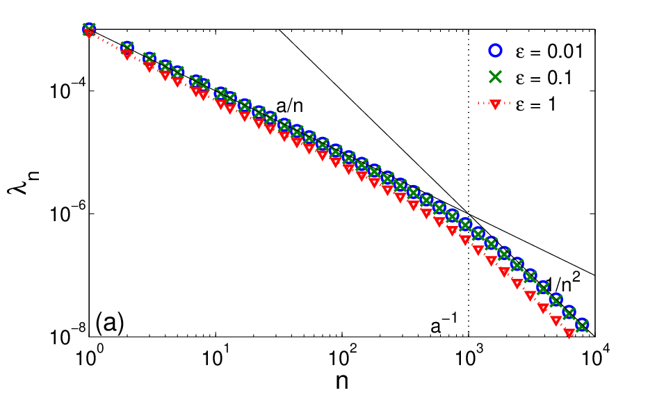
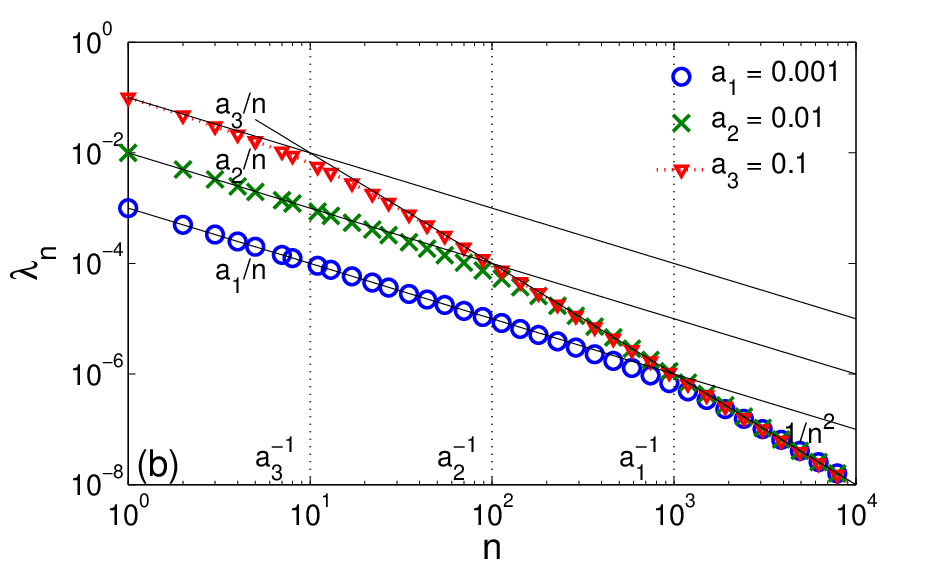
Fig. 2: Eignvalues λn\lambda_{n} of the operator V​T~​VV\tilde{T}V for (a) a=0.001a=0.001 and three values ϵ\epsilon: 0.010.01 (circles), 0.10.1 (crosses), and 11 (triangles); and (b) for ϵ=0.01\epsilon=0.01 and three values of aa: 0.0010.001 (circles), 0.010.01 (crosses), and 0.10.1 (triangles). Solid lines show the asymptotic relations a/na/n and 1/n21/n^{2}, while vertical dotted lines indicate the separation 1/a1/a between these asymptotic regimes. The coefficient AϵA_{\epsilon} in front of n−2n^{-2} relation is close to 11 for all small targets, except for ϵ=1\epsilon=1, see Eq. (38).

In this section, we analyze the case of extended targets (ϵ>0\epsilon>0) by numerical computations of the eigenvalues λn\lambda_{n} and the spectral weights ψn2\psi_{n}^{2} (see Appendix B for computational details). As for the point-like target, Figure 2 allows one to distinguish two regimes for λn\lambda_{n}, for small and large nn:

λn≃{A~a,ϵ​n−1(n≪1/a),Aϵ​n−2(n≫1/a),\lambda_{n}\simeq\begin{cases}\tilde{A}_{a,\epsilon}~n^{-1}\quad(n\ll 1/a),\cr A_{\epsilon}~n^{-2}\hskip 17.07164pt(n\gg 1/a),\end{cases} (37)

where A~a,ϵ\tilde{A}_{a,\epsilon} and AϵA_{\epsilon} are two constants. In Appendix A, we prove the second (large nn) asymptotic relation and show that the constant AϵA_{\epsilon} does not depend on aa. In turn, the transition between two asymptotic regimes is determined by 1/a1/a (and is independent of ϵ\epsilon). Note also that Aϵ→1A_{\epsilon}\to 1 as ϵ→0\epsilon\to 0 according to Eq. (36). One can see that these asymptotic relations accurately approximate the eigenvalues λn\lambda_{n}. The behavior of AϵA_{\epsilon} is shown on Fig. 4a. As expected, it does not depend on aa. These numerical results suggest the following conjectural expression:

Aϵ=(1−ϵ/π)2,A_{\epsilon}=(1-\epsilon/\pi)^{2}, (38)

which accurately reproduces AϵA_{\epsilon} on the whole range of ϵ\epsilon from 00 to π\pi. According to Eq. (35), the coefficient A~a,ϵ\tilde{A}_{a,\epsilon} is equal to aa when ϵ=0\epsilon=0. We plot therefore A~a,ϵ/a\tilde{A}_{a,\epsilon}/a on Fig. 4b, where this ratio approaches 11 as ϵ→0\epsilon\to 0, and 00 as ϵ→π\epsilon\to\pi. Moreover, this ratio weakly depends on aa (curves for a=0.001a=0.001 and a=0.1a=0.1 almost coincide).

Refer to caption
Refer to caption
Refer to caption
Fig. 3: Spectral weights ψn2\psi_{n}^{2} (shown by red solid line) for (a) a=0.001a=0.001 and ϵ=0.1\epsilon=0.1; (b) a=0.1a=0.1 and ϵ=0.001\epsilon=0.001; and (c) a=ϵ=0.01a=\epsilon=0.01. In the first two plots, three asymptotic regimes can be distinguished according to Eq. (39), while the intermediate regime disappears in the last plot.

Figure 3 shows that the asymptotic behavior of the spectral weights ψn2\psi_{n}^{2} is more complicated. One can distinguish three asymptotic regimes:

ψn2≃{B~a,ϵ​n−3(n≪min⁡{1/a,1/ϵ}),B~a,ϵ′​n−4(min⁡{1/a,1/ϵ}≪n≪max⁡{1/a,1/ϵ}),Ba,ϵ​n−6(n≫max⁡{1/a,1/ϵ}),\psi_{n}^{2}\simeq\begin{cases}\tilde{B}_{a,\epsilon}~n^{-3}\quad(n\ll\min\{1/a,1/\epsilon\}),\cr\tilde{B}^{\prime}_{a,\epsilon}~n^{-4}\quad(\min\{1/a,1/\epsilon\}\ll n\ll\max\{1/a,1/\epsilon\}),\cr B_{a,\epsilon}~n^{-6}\quad(n\gg\max\{1/a,1/\epsilon\}),\end{cases} (39)

In order to observe all three regimes, one needs 1≪min⁡{1/a,1/ϵ}≪max⁡{1/a,1/ϵ}1\ll\min\{1/a,1/\epsilon\}\ll\max\{1/a,1/\epsilon\}, i.e., either a≪ϵ≪1a\ll\epsilon\ll 1, or ϵ≪a≪1\epsilon\ll a\ll 1. For instance, if aa or ϵ\epsilon is not small enough, the first regime with n−3n^{-3} may not be well established (Fig. 3a, b). If a∼ϵa\sim\epsilon, the intermediate regime disappears, as illustrated on Fig. 3c. Finally, when ϵ→0\epsilon\to 0, max⁡{1/a,1/ϵ}→∞\max\{1/a,1/\epsilon\}\to\infty, the third regime disappears, and one retrieves two regimes for point-like targets.

The behavior of the coefficients Ba,ϵB_{a,\epsilon} and B~a,ϵ\tilde{B}_{a,\epsilon} is shown on Fig. 4c,d. As expected from Eq. (35), B~a,ϵ/(2​π​a)\tilde{B}_{a,\epsilon}/(2\pi a) approaches 11 as ϵ→0\epsilon\to 0 (point-like target). Moreover, such normalized coefficient weakly depends on aa (at least for small aa). The behavior of Ba,ϵB_{a,\epsilon} is more complicated. Given that 𝒯{\mathcal{T}} should converge to the mean exit time for pure bulk diffusion, ⟨t1⟩b\langle t_{1}\rangle_{b}, as a→0a\to 0, one gets

∑n≥1ψn2λn2≃2​π​D2​⟨t1⟩ba.\sum\limits_{n\geq 1}\frac{\psi_{n}^{2}}{\lambda_{n}^{2}}\simeq\frac{2\pi D_{2}\langle t_{1}\rangle_{b}}{a}. (40)

Since λn≃Aϵ​n−2\lambda_{n}\simeq A_{\epsilon}n^{-2} is independent of aa, one concludes that Ba,ϵ∼1/aB_{a,\epsilon}\sim 1/a as a→0a\to 0. For this reason, we plot a​Ba,ϵaB_{a,\epsilon} on Fig. 4c. For large ϵ\epsilon, two curves for a=0.001a=0.001 and a=0.1a=0.1 do coincide, as expected. However, strong deviations emerge at small ϵ\epsilon. In fact, one needs to consider much smaller aa to get coinciding curves over the whole considered range of ϵ\epsilon. We conclude that the reflection distance aa plays an important role, especially for small targets.

Although the above asymptotic regimes for λn\lambda_{n} and ψn2\psi_{n}^{2} remain conjectural, we will investigate their consequences for the asymptotic behavior of the mean exit time ⟨t1⟩\langle t_{1}\rangle. Using the asymptotic relations for large nn, we get

∑n≥1ψn2λn2​(λn+D1λ)\displaystyle\sum_{n\geq 1}{\frac{\psi_{n}^{2}}{\lambda_{n}^{2}\left(\lambda_{n}+\frac{D_{1}}{\lambda}\right)}} ∼∫1∞Ba,ϵ​x−6Aϵ2​x−4​(Aϵ​x−2+D1λ)​𝑑x\displaystyle\sim\int_{1}^{\infty}{\frac{B_{a,\epsilon}x^{-6}}{A_{\epsilon}^{2}x^{-4}\left(A_{\epsilon}x^{-2}+\frac{D_{1}}{\lambda}\right)}dx}
=Ba,ϵAϵ3​∫1∞d​x1+x2​D1λ​Aϵ∼Ba,ϵAϵ5/2​π2​λD1.\displaystyle=\frac{B_{a,\epsilon}}{A_{\epsilon}^{3}}\int_{1}^{\infty}{\frac{dx}{1+x^{2}\frac{D_{1}}{\lambda A_{\epsilon}}}}\sim\frac{B_{a,\epsilon}}{A_{\epsilon}^{5/2}}\frac{\pi}{2}\sqrt{\frac{\lambda}{D_{1}}}.

Consequently, we get

⟨t1⟩=𝒯−C1λ+O⁡(1λ),\displaystyle\langle t_{1}\rangle={\mathcal{T}}-\frac{C_{1}}{\sqrt{\lambda}}+O\left(\frac{1}{\lambda}\right), (41)

where

C1=Ca,ϵ​D1D2,Ca,ϵ=(1−(1−a)2)​Ba,ϵ8​Aϵ5/2.C_{1}=C_{a,\epsilon}~\frac{\sqrt{D_{1}}}{D_{2}},\qquad C_{a,\epsilon}=(1-(1-a)^{2})\frac{B_{a,\epsilon}}{8A_{\epsilon}^{5/2}}. (42)
Refer to caption
Refer to caption
Refer to caption
Refer to caption
Fig. 4: Coefficients AϵA_{\epsilon}, A~a,ϵ/a\tilde{A}_{a,\epsilon}/a, a​Ba,ϵaB_{a,\epsilon}, and B~a,ϵ/a\tilde{B}_{a,\epsilon}/a from Eqs. (37), (39) versus ϵ\epsilon. Two curves for a=0.001a=0.001 and a=0.1a=0.1 coincide that illustrates the independence of AϵA_{\epsilon} and A~ϵ/a\tilde{A}_{\epsilon}/a of aa.

For an accurate numerical computation of ⟨t1⟩\langle t_{1}\rangle, we consider the behavior of partial sums f⁡(N)=∑n=1Nψn2λn​(D1λ+λn)f(N)=\sum_{n=1}^{N}\frac{\psi_{n}^{2}}{\lambda_{n}\left(\frac{D_{1}}{\lambda}+\lambda_{n}\right)} (note that ⟨t1⟩\langle t_{1}\rangle is obtained in the limit N→∞N\to\infty according to Eq. (30)). We checked that f⁡(N)∼f⁡(∞)+cNf(N)\sim f(\infty)+\frac{c}{N} for large NN (for a fixed λ\lambda). In practice, we used the fourth order polynomial fit of f⁡(N)f(N) versus 1/N1/N for NN from 1000 to 20000 to extrapolate the value f⁡(∞)f(\infty).

Figure 5 shows the mean exit time ⟨t1⟩\langle t_{1}\rangle as a function of λ\lambda for a small target (ϵ=0.01\epsilon=0.01) and two values of aa: 0.010.01 and 0.0010.001. In both cases, the mean exit time passes through a minimum at some intermediate desorption rate λc\lambda_{c} and then approaches the maximum as λ→∞\lambda\to\infty. One can clearly see that the optimal value λc\lambda_{c}, as well as the height of the maximum at λ→∞\lambda\to\infty, depend on aa. Although both considered values a=0.001a=0.001 and a=0.01a=0.01 are small, the limiting mean exit time 𝒯{\mathcal{T}} changes significantly. The asymptotic relation (41) (shown by thin solid lines) accurately captures the limiting behavior.

Refer to caption
Fig. 5: The mean exit time ⟨t1⟩\langle t_{1}\rangle as a function of λ\lambda for ϵ=0.01\epsilon=0.01, D1=D2=1D_{1}=D_{2}=1, and two values of aa: 0.010.01 (solid line) and 0.0010.001 (dashed line). Two horizontal lines indicate the mean exit times for surface diffusion ⟨t1⟩λ=0≈3.2586\langle t_{1}\rangle_{\lambda=0}\approx 3.2586 and for pure bulk diffusion ⟨t1⟩λ=∞≈5.2929\langle t_{1}\rangle_{\lambda=\infty}\approx 5.2929 from Eqs. (29), (70). Thin lines show the asymptotic behavior (41) where 𝒯{\mathcal{T}} and C1C_{1} are computed from Eqs. (31), (42).

When ϵ→0\epsilon\to 0, we use Eqs. (37) and (39) to get

𝒯\displaystyle{\mathcal{T}} =1−(1−a)24​π​D2​∑n≥1ψn2λn2=1−(1−a)24​π​D2​(∑n=11/ϵB~a,ϵ​n−3A~a,ϵ2​n−2+O⁡(ϵ))\displaystyle=\frac{1-(1-a)^{2}}{4\pi D_{2}}\sum_{n\geq 1}{\frac{\psi_{n}^{2}}{\lambda_{n}^{2}}}=\frac{1-(1-a)^{2}}{4\pi D_{2}}\left(\sum_{n=1}^{1/\epsilon}\frac{\tilde{B}_{a,\epsilon}n^{-3}}{\tilde{A}_{a,\epsilon}^{2}n^{-2}}+O(\epsilon)\right)
=1−(1−a)24​π​D2​(B~a,ϵA~a,ϵ2​ln⁡1ϵ+O⁡(ϵ)).\displaystyle=\frac{1-(1-a)^{2}}{4\pi D_{2}}\left(\frac{\tilde{B}_{a,\epsilon}}{\tilde{A}_{a,\epsilon}^{2}}\ln\frac{1}{\epsilon}+O(\epsilon)\right). (43)

This logarithmic divergence is similar to the result from Ref. [21, 19, 20] which describes the mean exit time for non-intermittent pure bulk diffusion (2D Brownian motion) in the narrow escape limit (ϵ→0\epsilon\to 0). This case formally corresponds to the double limit λ→∞\lambda\to\infty and a→0a\to 0. Interestingly, the double limit can be taken separately: as λ→∞\lambda\to\infty, the limiting value 𝒯{\mathcal{T}} exists for any finite aa. In this way, we extended the classical escape problem for pure bulk diffusion by including reflections at a finite distance aa. In Appendix C, we provide the exact formula for the mean exit time for pure bulk diffusion ⟨t1⟩b\langle t_{1}\rangle_{b}. In the narrow escape limit ϵ→0\epsilon\to 0, one gets ⟨t1⟩b≈ln⁡(2/ϵ)D2​(1+O⁡(ϵ))\langle t_{1}\rangle_{b}\approx\frac{\ln(2/\epsilon)}{D_{2}}\bigl(1+O(\epsilon)\bigr).

Figure 6 shows the dependence of the limiting mean exit time 𝒯{\mathcal{T}} on aa and ϵ\epsilon. For fixed target size ϵ\epsilon, 𝒯{\mathcal{T}} approaches the mean exit time for pure bulk diffusion ⟨t1⟩b\langle t_{1}\rangle_{b} as a→0a\to 0 (Fig. 6a). Note that a simple formula for 𝒯{\mathcal{T}} in the special case a=1a=1 is derived in Appendix D. For fixed reflection distance aa, 𝒯{\mathcal{T}} exhibits the logarithmic dependence on ϵ\epsilon for ϵ≳a\epsilon\gtrsim a, in agreement with Eq. (43). In the opposite case ϵ≲a\epsilon\lesssim a, the reflection distance aa alters this behavior.

Refer to caption
Refer to caption
Fig. 6: (a) The limiting mean exit time 𝒯{\mathcal{T}} as a function of aa for ϵ=0.01\epsilon=0.01 (circles) and ϵ=0.1\epsilon=0.1 (crosses), D2=1D_{2}=1. Two horizontal lines indicate the mean exit time for pure bulk diffusion ⟨t1⟩λ=∞\langle t_{1}\rangle_{\lambda=\infty}: 5.29295.2929 and 2.99492.9949, respectively. As expected, 𝒯{\mathcal{T}} increases with aa because every reflection from the boundary by distance aa requires additional time to return (given that the target is located at the boundary). In the limit a=1a=1, 𝒯{\mathcal{T}} becomes 78.289878.2898 for ϵ=0.01\epsilon=0.01 and 7.60407.6040 for ϵ=0.1\epsilon=0.1 according to Eq. (71). (b) 𝒯{\mathcal{T}} as a function of ϵ\epsilon for a=0.001a=0.001 (pluses) and a=0.01a=0.01 (circles). Solid line shows the mean exit time for pure bulk diffusion from Eq. (70). As expected, the limiting time diverges logarithmically with ϵ\epsilon when ϵ≳a\epsilon\gtrsim a. In the opposite case ϵ≲a\epsilon\lesssim a, the reflection distance aa alters this behavior.

4 Diagonal approximation

In [3], an explicit diagonal approximation to the mean exit time has been proposed and checked numerically to be accurate. In our notations, this approximation consists in removing all nondiagonal elements of the matrix 𝐕𝐓𝐕{\bf V}{\bf T}{\bf V} from Eq. (63) that represents the operator V​T~​VV\tilde{T}V in the cosine basis. Under this approximation, one gets

λn≈1−(1−a)nn2​π−ϵ+sin⁡2​n​ϵ2​nπ,en≈2π​cos⁡(n​θ),\lambda_{n}\approx\frac{1-(1-a)^{n}}{n^{2}}~\frac{\pi-\epsilon+\frac{\sin 2n\epsilon}{2n}}{\pi},\qquad e_{n}\approx\sqrt{\frac{2}{\pi}}\cos(n\theta), (44)

from which

ψn2≈2​(1−(1−a)n)π​n4​((π−ϵ)​cos⁡n​ϵ+sin⁡n​ϵn)2.\psi_{n}^{2}\approx\frac{2(1-(1-a)^{n})}{\pi n^{4}}\biggl((\pi-\epsilon)\cos n\epsilon+\frac{\sin n\epsilon}{n}\biggr)^{2}. (45)

Substituting these approximations into Eq. (15), we retrieve the diagonal approximation from [3]:

⟨t1⟩≈1π​D1(1+λ1−(1−a)24​D2)[(π−ϵ)33−2​λπ​D1∑n≥11−(1−a)nn2((π−ϵ)​cos⁡n​ϵ+sin⁡n​ϵn)2n2+λπ​D1​(1−(1−a)n)​(π−ϵ+sin⁡2​n​ϵ2​n)].\begin{split}\langle t_{1}\rangle&\approx\frac{1}{\pi D_{1}}\left(1+\lambda\frac{1-(1-a)^{2}}{4D_{2}}\right)\biggl[\frac{(\pi-\epsilon)^{3}}{3}\\ &-\frac{2\lambda}{\pi D_{1}}\sum\limits_{n\geq 1}\frac{1-(1-a)^{n}}{n^{2}}\frac{\bigl((\pi-\epsilon)\cos n\epsilon+\frac{\sin n\epsilon}{n}\bigr)^{2}}{n^{2}+\frac{\lambda}{\pi D_{1}}(1-(1-a)^{n})\bigl(\pi-\epsilon+\frac{\sin 2n\epsilon}{2n}\bigr)}\biggr].\\ \end{split} (46)

The diagonal approximation has been shown numerically to be very accurate for moderate λ\lambda and arbitrary ϵ\epsilon (see [3]). Although the matrix 𝐕𝐓𝐕{\bf V}{\bf T}{\bf V} has indeed the dominant diagonal, the remarkable quality of this approximation remained puzzling. At the same time, the approximation becomes inappropriate in the limit of large λ\lambda. In order to get a finite limit of the mean exit time for ϵ>0\epsilon>0 as λ→∞\lambda\to\infty, the constant term (π−ϵ)3/3(\pi-\epsilon)^{3}/3 has to be compensated. In other words, writing Eq. (46) as

⟨t1⟩≈1π​D1(1+λ1−(1−a)24​D2){[(π−ϵ)33−2∑n≥1((π−ϵ)​cos⁡n​ϵ+sin⁡n​ϵn)2π−ϵ+sin⁡2​n​ϵ2​n1n2]+2∑n≥1((π−ϵ)​cos⁡n​ϵ+sin⁡n​ϵn)2π−ϵ+sin⁡2​n​ϵ2​n1n2+λπ​D1​(1−(1−a)n)​(π−ϵ+sin⁡2​n​ϵ2​n)},\begin{split}\langle t_{1}\rangle&\approx\frac{1}{\pi D_{1}}\left(1+\lambda\frac{1-(1-a)^{2}}{4D_{2}}\right)\biggl\{\biggl[\frac{(\pi-\epsilon)^{3}}{3}-2\sum\limits_{n\geq 1}\frac{\bigl((\pi-\epsilon)\cos n\epsilon+\frac{\sin n\epsilon}{n}\bigr)^{2}}{\pi-\epsilon+\frac{\sin 2n\epsilon}{2n}}\frac{1}{n^{2}}\biggr]\\ &+2\sum\limits_{n\geq 1}\frac{\bigl((\pi-\epsilon)\cos n\epsilon+\frac{\sin n\epsilon}{n}\bigr)^{2}}{\pi-\epsilon+\frac{\sin 2n\epsilon}{2n}}\frac{1}{n^{2}+\frac{\lambda}{\pi D_{1}}(1-(1-a)^{n})\bigl(\pi-\epsilon+\frac{\sin 2n\epsilon}{2n}\bigr)}\biggr\},\\ \end{split} (47)

the constant term in square brackets should be canceled. This is true only for ϵ=0\epsilon=0 and ϵ=π\epsilon=\pi. As a consequence, the diagonal approximation (46) (or (47)) implies the divergence of the mean exit time as λ→∞\lambda\to\infty, in contrast to the expected convergence to a finite limit for ϵ>0\epsilon>0.

This discrepancy can be interpreted in terms of the asymptotic behavior of the spectral weights ψn2\psi_{n}^{2}. In fact, the approximate relation (45) suggests ψn2∝n−4\psi_{n}^{2}\propto n^{-4}, in contrast to the observed n−6n^{-6} decay. In other words, the diagonal approximation operates over an intermediate asymptotic regime, while the ultimate n−6n^{-6} asymptotics is missed. This observation explains why the diagonal approximation accurately captures the behavior of the mean exit time ⟨t1⟩\langle t_{1}\rangle over small and moderate λ\lambda but fails in the limit λ→∞\lambda\to\infty (see Fig. 1b).

Conclusion

In summary, we presented a spectral approach for computing the mean exit time ⟨t1⟩\langle t_{1}\rangle from the unit disk by surface-mediated diffusion with two alternating phases of bulk and surface motion. The derived spectral representation is particularly suitable for the asymptotic analysis of the mean exit time in the limit of large desorption rates λ\lambda. For a point-like target (ϵ=0\epsilon=0), we proved the asymptotic increase ⟨t1⟩∝λ\langle t_{1}\rangle\propto\sqrt{\lambda} and provided lower and upper bounds. For extended targets (ϵ>0\epsilon>0), we investigated the asymptotic approach of the mean exit time to a finite limit and proved an increase of ⟨t1⟩\langle t_{1}\rangle at large λ\lambda (the first correction term being ∝λ−1/2\propto\lambda^{-1/2}). We revealed different asymptotic behaviors of the governing eigenvalues λn\lambda_{n} and spectral weights ψn2\psi_{n}^{2} depending on the target size ϵ\epsilon and the reflection distance aa. Finally, we discussed the optimality of surface-mediated diffusion and potential limitations of the diagonal approximation for the mean exit time.

5 Appendices

Appendix A Asymptotic behavior of the eigenvalues of the operator V​T~​VV\tilde{T}V

Theorem 3.

Let λn\lambda_{n} be the eigenvalues of the operator V​T~​VV\tilde{T}V, where the operators T~\tilde{T} and VV are defined in Eqs. (7) and (6). We have

λn∼Aϵ​n−2,\lambda_{n}\sim A_{\epsilon}n^{-2}, (48)

where AϵA_{\epsilon} depends only on ϵ\epsilon.

Proof.

In order to prove this statement, we first investigate the following problem:

Let AA and BB are two compact, positive, self-adjoint operators. We assume that the eigenvalues of the operator AA are ordered in a decreasing sequence: λ1​(A)≥λ2​(A)≥…≥λn​(A)≥…≥0\lambda_{1}(A)\geq\lambda_{2}(A)\geq\ldots\geq\lambda_{n}(A)\geq\ldots\geq 0. We recall the variational principle as following

Theorem 4.
λn(A)=maxFminO≠x∈A⟨A​x,x⟩⟨x,x⟩;(where F is a subspaces of L2[0,π]; dimF=n).\lambda_{n}(A)=\max_{F}\min_{O\neq x\in A}\frac{\langle Ax,x\rangle}{\langle x,x\rangle};\text{(}\text{where }F\text{ is a subspaces of }L^{2}[0,\pi];\text{ }\dim F=n\text{)}. (49)

The max\max is taken over FF, the subspace associated with the first nn eigenvectors of AA.

We state two following lemmas which will be needed to prove the proposition 3.

Lemma 5.

We make the assumption that λn​(A)\lambda_{n}(A), λn​(A+B)\lambda_{n}(A+B) are the nt​hn^{th} eigenvalues of the operators AA and A+BA+B. Then, we have

λn​(A)−‖B‖≤λn​(A+B)≤λn​(A)+‖B‖,\lambda_{n}(A)-\|B\|\leq\lambda_{n}(A+B)\leq\lambda_{n}(A)+\|B\|, (50)

where ∥.∥\|.\| define the norm of an operator in L2​[0,π]L^{2}[0,\pi] space.

Proof.

Let FF be the subspace of L2​[0,π]L^{2}[0,\pi] associated with the first nn eigenvectors of AA. For all x∈Fx\in F, we have

⟨(A+B)​x,x⟩=⟨A​x,x⟩+⟨B​x,x⟩.\displaystyle\langle(A+B)x,x\rangle=\langle Ax,x\rangle+\langle Bx,x\rangle.

According to the variational principle, we have

⟨A​x,x⟩≥minx∈A⁡⟨A​x,x⟩⟨x,x⟩​‖x‖2=λn​(A)​‖x‖2.\displaystyle\langle Ax,x\rangle\geq\min_{x\in A}\frac{\langle Ax,x\rangle}{\langle x,x\rangle}\|x\|^{2}=\lambda_{n}(A)\|x\|^{2}. (51)

Besides, we have

|⟨B​x,x⟩|≤‖B‖​‖x‖2.\displaystyle|\langle Bx,x\rangle|\leq\|B\|\|x\|^{2}. (52)

It follows from Eqs. (51) and (52) that

⟨(A+B)​x,x⟩≥λn​(A)​‖x‖2−‖B‖​‖x‖2.\displaystyle\langle(A+B)x,x\rangle\geq\lambda_{n}(A)\|x\|^{2}-\|B\|\|x\|^{2}.

This gives

min0≠x∈F⁡⟨(A+B)​x,x⟩‖x‖2≥λn​(A)−‖B‖.\displaystyle\min_{0\neq x\in F}\frac{\langle(A+B)x,x\rangle}{\|x\|^{2}}\geq\lambda_{n}(A)-\|B\|.

Again, according to the variational principle, we thus get

λn​(A+B)≥λn​(A)−‖B‖.\displaystyle\lambda_{n}(A+B)\geq\lambda_{n}(A)-\|B\|.

In the same manner, if we take FF be associated to the first nn eigenvectors of A+BA+B, we can get

λn​(A+B)≤λn​(A)+‖B‖,\displaystyle\lambda_{n}(A+B)\leq\lambda_{n}(A)+\|B\|,

and the lemma 5 follows. ∎

Lemma 6.

With the notations used in lemma 5, if rank⁡(B)<∞{\rm rank}(B)<\infty, then

λn+rank⁡(B)​(A)≤λn​(A+B)≤λn−rank⁡(B)​(A).\lambda_{n+{\rm rank}(B)}(A)\leq\lambda_{n}(A+B)\leq\lambda_{n-{\rm rank}(B)}(A). (53)
Proof.

We call FF the subspace of L2​[0,π]L^{2}[0,\pi] associated with the first n−rank⁡(B)n-{\rm rank}(B) eigenvectors of AA.

By the variational principle, we have

∀x∈F∩ker⁡(B),‖x‖=1:⟨(A+B)​x,x⟩=⟨A​x,x⟩≥λn+rank⁡(B)​(A).\forall x\in F\cap\ker(B),\|x\|=1:\langle(A+B)x,x\rangle=\langle Ax,x\rangle\geq\lambda_{n+{\rm rank}(B)}(A).

Consequently,

minx∈F∩ker⁡(B);‖x‖=1⁡⟨(A+B)​x,x⟩≥λn+rank⁡(B)​(A).\min_{x\in F\cap\ker(B);\\ \|x\|=1}\langle(A+B)x,x\rangle\geq\lambda_{n+{\rm rank}(B)}(A).

Since

dim(F∩ker⁡(B))=dimF−dimB⁡(F)≥n,\dim(F\cap\ker(B))=\dim F-\dim B(F)\geq n,

we have

λn​(A+B)≥min0≠x∈ker⁡(B)∩F;‖x‖=1⁡⟨(A+B)​x,x⟩.\lambda_{n}(A+B)\geq\min_{0\neq x\in\ker(B)\cap F;\\ \|x\|=1}\langle(A+B)x,x\rangle.

So, we conclude that

λn​(A+B)≥λn+rank⁡(B)​(A).\lambda_{n}(A+B)\geq\lambda_{n+{\rm rank}(B)}(A). (54)

The second inequality in (53) of this lemma is obtained when we put A′=A+BA^{\prime}=A+B, B′=−BB^{\prime}=-B, n′=n−rank⁡(B)n^{\prime}=n-{\rm rank}(B) and apply the conclusion (54) for A′A^{\prime}, B′B^{\prime} and n′n^{\prime} instead of AA, BB and nn. ∎

We now call πN\pi_{N} be the orthogonal projection on the first NN eigenvectors of BB.

By the property of an orthogonal projection, we can rewrite

B=πN​B​πN+(I−πN)​B​(I−πN),B=\pi_{N}B\pi_{N}+(I-\pi_{N})B(I-\pi_{N}),

then

A+B=A+πN​B​πN+(I−πN)​B​(I−πN).A+B=A+\pi_{N}B\pi_{N}+(I-\pi_{N})B(I-\pi_{N}).

We note that

rank⁡(πN​B​πN)=N,\displaystyle{\rm rank}(\pi_{N}B\pi_{N})=N,

and

‖(I−πN)​B​(I−πN)‖≤λN​(B).\displaystyle\|(I-\pi_{N})B(I-\pi_{N})\|\leq\lambda_{N}(B). (55)

By applying lemma 5, we get ∀n≥N\forall~n\geq N,

λn​(A+πN​B​πN)−‖(I−πN)​B​(I−πN)‖≤λn​(A+B),\displaystyle\lambda_{n}(A+\pi_{N}B\pi_{N})-\|(I-\pi_{N})B(I-\pi_{N})\|\leq\lambda_{n}(A+B),
λn​(A+B)≤λn​(A+πN​B​πN)+‖(I−πN)​B​(I−πN)‖.\displaystyle\lambda_{n}(A+B)\leq\lambda_{n}(A+\pi_{N}B\pi_{N})+\|(I-\pi_{N})B(I-\pi_{N})\|.

From (55), we obtain

λn​(A+πN​B​πN)−λN​(B)≤λn​(A+B)≤λn​(A+πN​B​πN)+λN​(B).\displaystyle\lambda_{n}(A+\pi_{N}B\pi_{N})-\lambda_{N}(B)\leq\lambda_{n}(A+B)\leq\lambda_{n}(A+\pi_{N}B\pi_{N})+\lambda_{N}(B).

According to lemma 6,

λn+N​(A)−λN​(B)≤λn​(A+B)≤λn−N​(A)+λN​(B).\displaystyle\lambda_{n+N}(A)-\lambda_{N}(B)\leq\lambda_{n}(A+B)\leq\lambda_{n-N}(A)+\lambda_{N}(B).

We can thus conclude that

∀N, ∀n≥N: λn+N(A)−λN(B)≤λn(A+B)≤λn−N(A)+λN(B).\displaystyle\forall N,\text{ }\forall n\geq N:\text{ }\lambda_{n+N}(A)-\lambda_{N}(B)\leq\lambda_{n}(A+B)\leq\lambda_{n-N}(A)+\lambda_{N}(B). (56)
Lemma 7.

Let {λn​(A)}\{\lambda_{n}(A)\} and {λn​(B)}\{\lambda_{n}(B)\} are the eigenvalues of two self-adjoint operators AA and BB. If λn​(A)∼c​n−s\lambda_{n}(A)\sim cn^{-s} and λN​(B)=ρN\lambda_{N}(B)=\rho^{N} where AA and ρ\rho are some constants, 0≤ρ≤10\leq\rho\leq 1, then

λn​(A+B)∼c​n−s.\displaystyle\lambda_{n}(A+B)\sim cn^{-s}.
Proof.

Indeed, by applying (56), if we choose N⁡(n)=nδN(n)=n^{\delta}, with δ<1\delta<1, then we obtain from (56) that

c​(n+nδ)−s​(1+o⁡(1))−ρnδ≤λn​(A+B)≤c​(n−nδ)−s​(1+o⁡(1))+ρnδ,\displaystyle c(n+n^{\delta})^{-s}(1+o(1))-\rho^{n^{\delta}}\leq\lambda_{n}(A+B)\leq c(n-n^{\delta})^{-s}(1+o(1))+\rho^{n^{\delta}},

Let n→∞n\rightarrow\infty, we have

c​n−s​(1+o⁡(1))≤λn​(A+B)≤c​n−s​(1+o⁡(1)).\displaystyle cn^{-s}(1+o(1))\leq\lambda_{n}(A+B)\leq cn^{-s}(1+o(1)).

Hence, we conclude that λn​(A+B)∼c​n−s\lambda_{n}(A+B)\sim cn^{-s}. ∎

We now turn back to prove the Proposition 3.

We consider the eigenpairs of the operator V​T~​VV\tilde{T}V, where T~\tilde{T} is defined in Eq. (7), and VV is defined by

V⁡(cos⁡n​x)=1−(1−a)n​cos⁡n​x≃(1−12​(1−a)n)​cos⁡n​x\displaystyle V(\cos nx)=\sqrt{1-(1-a)^{n}}\cos nx\simeq\left(1-\frac{1}{2}(1-a)^{n}\right)\cos nx

(the last approximate equality is valid for a≪1a\ll 1). We note that VV and T~\tilde{T} are self-adjoint operators. We rewrite VV as I−RI-R where

R⁡(cos⁡n​x)=12​(1−a)n​cos⁡n​x,\displaystyle R(\cos nx)=\frac{1}{2}(1-a)^{n}\cos nx,

then,

V​T~​V=(I−R)​T~​(I−R)=T~−R​T~−T~​R−R​T~​R.\displaystyle V\tilde{T}V=(I-R)\tilde{T}(I-R)=\tilde{T}-R\tilde{T}-\tilde{T}R-R\tilde{T}R.

Let us denote by KNK_{N} the image of the orthonormal projection on the first NthN^{\rm th} eigenvectors of RR and RNR_{N} the image of the orthonormal projection on the rest eigenvectors of RR. By definition, R=KN+RNR=K_{N}+R_{N}. Then,

V​T~​V\displaystyle V\tilde{T}V =T~−(KN+RN)​T~−T~​(KN+RN)+(KN+RN)​T~​(KN+RN)\displaystyle=\tilde{T}-(K_{N}+R_{N})\tilde{T}-\tilde{T}(K_{N}+R_{N})+(K_{N}+R_{N})\tilde{T}(K_{N}+R_{N})
=T~​−KN​T~−T~​KN+KN​T~​KN+KN​T~​RN+RN​T~​KN⏟these operators have the finite rank, which equal to ​N−RN​T~−T~​RN+RN​T~​RN.\displaystyle=\tilde{T}\underbrace{-K_{N}\tilde{T}-\tilde{T}K_{N}+K_{N}\tilde{T}K_{N}+K_{N}\tilde{T}R_{N}+R_{N}\tilde{T}K_{N}}_{\text{these operators have the finite rank, which equal to }N}-R_{N}\tilde{T}-\tilde{T}R_{N}+R_{N}\tilde{T}R_{N}. (57)

We note that rank⁡(KN)=N{\rm rank}(K_{N})=N and in formula (57), whenever there is a KNK_{N}, we have an operator of rank NN. Moreover, −RN​T~−T~​RN+RN​T~​RN-R_{N}\tilde{T}-\tilde{T}R_{N}+R_{N}\tilde{T}R_{N} has the norm dominated by the NthN^{\rm th} eigenvalue of RR:

‖−RN​T~−T~​RN+RN​T~​RN‖\displaystyle\|-R_{N}\tilde{T}-\tilde{T}R_{N}+R_{N}\tilde{T}R_{N}\| ≤‖RN​T~‖+‖T~​RN‖+‖RN​T~​RN‖\displaystyle\leq\|R_{N}\tilde{T}\|+\|\tilde{T}R_{N}\|+\|R_{N}\tilde{T}R_{N}\|
≤c​‖RN‖≤c​λN​(R)=c2​(1−a)N.\displaystyle\leq c\|R_{N}\|\leq c\lambda_{N}(R)=\frac{c}{2}(1-a)^{N}.

Since the operator T~\tilde{T} is the solution of the Sturm-Liouville problem, λn​(T~)∼Aϵ​n−2\lambda_{n}(\tilde{T})\sim A_{\epsilon}n^{-2}. Hence, refer to lemma 7, we get that

λn​(V​T~​V)∼Aϵ​n−2.\displaystyle\lambda_{n}(V\tilde{T}V)\sim A_{\epsilon}n^{-2}.

∎

Appendix B Numerical computation of spectral characteristics

We briefly present a numerical algorithm to compute the spectral characteristics λn\lambda_{n} and ψn\psi_{n}. In order to compute the eigenvalues λn\lambda_{n} and the eigenvectors ene_{n} of the operator V​T~​VV\tilde{T}V, we get an explicit representation of this operator in the basis cos⁡n​θ\cos n\theta. First, we find

T~​(cos⁡n​θ)={cos⁡n​θ−cos⁡n⁡(π−ϵ)n2,0≤θ<π−ϵ,0,π−ϵ≤θ≤π,\tilde{T}(\cos n\theta)=\begin{cases}\frac{\cos n\theta-\cos n(\pi-\epsilon)}{n^{2}},&0\leq\theta<\pi-\epsilon,\\ 0,&\pi-\epsilon\leq\theta\leq\pi,\end{cases} (58)

and

T~​(1)​(θ)={(π−ϵ)2−θ22,0≤θ<π−ϵ,0,π−ϵ≤θ≤π,\tilde{T}(1)(\theta)=\begin{cases}\frac{(\pi-\epsilon)^{2}-\theta^{2}}{2},&0\leq\theta<\pi-\epsilon,\\ 0,&\pi-\epsilon\leq\theta\leq\pi,\end{cases} (59)

from which the expansion of T~​(cos⁡n​θ)\tilde{T}(\cos n\theta) (n≥0n\geq 0) in the basis {cos⁡n​θ}\{\cos n\theta\} of Leven2​[0,π]L_{\text{even}}^{2}{[0,\pi]} is

T~​(cos⁡n​θ)=∑m≥0𝐓m​n​cos⁡m​θn≥0,\tilde{T}(\cos n\theta)=\sum_{m\geq 0}{\bf T}_{mn}\cos m\theta\quad n\geq 0, (60)

where the coefficients 𝐓m​n{\bf T}_{mn} are defined by

π2​𝐓m​n\displaystyle\frac{\pi}{2}{\bf T}_{mn} ={⟨T~​(cos⁡n​θ),cos⁡m​θ⟩, if ​m≥112​⟨T~​(cos⁡n​θ),1⟩, if ​m=0\displaystyle=\begin{cases}\langle\tilde{T}(\cos n\theta),\cos m\theta\rangle,&\text{ if }m\geq 1\\ \frac{1}{2}\langle\tilde{T}(\cos n\theta),1\rangle,&\text{ if }m=0\end{cases}
={12​(1−δm​n)​(−1)m+n+1m​n​[sin⁡(m−n)​ϵm−n−sin⁡(m+n)​ϵm+n]+12​δm​n​1n2​(π−ϵ+sin⁡2​n​ϵ2​n)(m≥1,n≥1),12​(−1)n+1n2​[(π−ϵ)​cos⁡n​ϵ+sin⁡n​ϵn],(m=0,n≥1),(−1)m+1m2​[(π−ϵ)​cos⁡m​ϵ+sin⁡m​ϵm],(m≥1,n=0),(π−ϵ)36,(m=0,n=0).\displaystyle=\begin{cases}\frac{1}{2}(1-\delta_{mn})\frac{(-1)^{m+n+1}}{mn}\biggl[\frac{\sin(m-n)\epsilon}{m-n}-\frac{\sin(m+n)\epsilon}{m+n}\biggr]+\frac{1}{2}\delta_{mn}\frac{1}{n^{2}}\left(\pi-\epsilon+\frac{\sin 2n\epsilon}{2n}\right)\\ \hskip 227.62204pt(m\geq 1;~n\geq 1),\\ \frac{1}{2}\frac{(-1)^{n+1}}{n^{2}}\left[(\pi-\epsilon)\cos n\epsilon+\frac{\sin n\epsilon}{n}\right],\hskip 85.35826pt(m=0;~n\geq 1),\\ \frac{(-1)^{m+1}}{m^{2}}\left[(\pi-\epsilon)\cos m\epsilon+\frac{\sin m\epsilon}{m}\right],\hskip 79.66771pt(m\geq 1;~n=0),\\ \frac{(\pi-\epsilon)^{3}}{6},\hskip 197.74664pt(m=0;~n=0).\end{cases} (61)

In turn, the operator VV has a diagonal representation:

𝐕m​n={1−(1−a)m(m=n,m,n≥0),0(m≠n,m,n≥0).\displaystyle{\bf V}_{mn}=\begin{cases}\sqrt{1-(1-a)^{m}}&(m=n;~m,n\geq 0),\\ 0&(m\neq n;~m,n\geq 0).\end{cases} (62)

Combining these results, the operator V​T~​VV\tilde{T}V is represented by the infinite-dimensional matrix 𝐕𝐓𝐕{\bf V}{\bf T}{\bf V} whose elements are

[𝐕𝐓𝐕]m,n\displaystyle[{\bf V}{\bf T}{\bf V}]_{m,n} =1π1−(1−a)n1−(1−a)m{δm​n1n2(π−ϵ+sin⁡2​n​ϵ2​n)\displaystyle=\frac{1}{\pi}\sqrt{1-(1-a)^{n}}~\sqrt{1-(1-a)^{m}}\biggl\{\delta_{mn}\frac{1}{n^{2}}\left(\pi-\epsilon+\frac{\sin 2n\epsilon}{2n}\right) (63)
−(1−δm​n)(−1)m+nm​n[sin⁡(m−n)​ϵm−n−sin⁡(m+n)​ϵm+n]}(m≥1;n≥1),\displaystyle-(1-\delta_{mn})\frac{(-1)^{m+n}}{mn}\biggl[\frac{\sin(m-n)\epsilon}{m-n}-\frac{\sin(m+n)\epsilon}{m+n}\biggr]\biggr\}\quad(m\geq 1;~n\geq 1),

and [𝐕𝐓𝐕]m,n=0[{\bf V}{\bf T}{\bf V}]_{m,n}=0 if m=0m=0 or n=0n=0. Solving the eigenvalues {λn}\{\lambda_{n}\} and the eigenvectors {en}\{e_{n}\} of the operator V​T~​VV\tilde{T}V is equivalent to finding the eigenpairs of the associated matrix 𝐕𝐓𝐕{\bf V}{\bf T}{\bf V}. Note that this matrix is symmetric.

The matrix 𝐕𝐓𝐕{\bf V}{\bf T}{\bf V} is diagonalized in Matlab that finds the eigenvalues λn\lambda_{n} and the coefficients vm​nv_{mn} determining the orthonormal basis {en}n≥0\{e_{n}\}_{n\geq 0} as

en​(θ)=1π​v0​n+2π​∑m≥1vm​n​cos⁡m​θ.e_{n}(\theta)=\sqrt{\frac{1}{\pi}}~v_{0n}+\sqrt{\frac{2}{\pi}}\sum_{m\geq 1}v_{mn}\cos m\theta. (64)

The spectral weights ψn\psi_{n} are then given as

ψn=⟨ψ,en⟩=2π​∑m≥1vm​n​⟨ψ,cos⁡m​θ⟩,\displaystyle\psi_{n}=\langle\psi,e_{n}\rangle=\sqrt{\frac{2}{\pi}}\sum_{m\geq 1}v_{mn}\langle\psi,\cos m\theta\rangle, (65)

where

⟨ψ,cos⁡m​θ⟩=1−(1−a)m​(−1)m+1m2​[(π−ϵ)​cos⁡m​ϵ+sin⁡m​ϵm],\displaystyle\langle\psi,\cos m\theta\rangle=\sqrt{1-(1-a)^{m}}~\frac{(-1)^{m+1}}{m^{2}}\left[(\pi-\epsilon)\cos m\epsilon+\frac{\sin m\epsilon}{m}\right],

and ⟨ψ,1⟩=⟨V​T~​(1),1⟩=⟨T~​(1),V​1⟩=0\langle\psi,1\rangle=\langle V\tilde{T}(1),1\rangle=\langle\tilde{T}(1),V1\rangle=0.

Appendix C Pure bulk diffusion phase

In [15], the mean exit time for pure bulk diffusion phase (λ=∞\lambda=\infty, a=0a=0) was found to be

t2​(r,θ)=1D2​(1−r24+α02+∑n=1∞αn​rn​cos⁡n​θ),t_{2}(r,\theta)=\frac{1}{D_{2}}\left(\frac{1-r^{2}}{4}+\frac{\alpha_{0}}{2}+\sum\limits_{n=1}^{\infty}\alpha_{n}r^{n}\cos n\theta\right), (66)

where

α0\displaystyle\alpha_{0} =−2​ln⁡[sin⁡(ϵ/2)],\displaystyle=-2\ln[\sin(\epsilon/2)], (67)
αn\displaystyle\alpha_{n} =(−1)n−12​n​[Pn​(cos⁡ϵ)+Pn−1​(cos⁡ϵ)],\displaystyle=\frac{(-1)^{n-1}}{2n}\bigl[P_{n}(\cos\epsilon)+P_{n-1}(\cos\epsilon)\bigr], (68)

where Pn​(z)P_{n}(z) are Legendre polynomials. In the limit r→1r\to 1, one gets

t1​(θ)={1D2​(12​α0+∑n=1∞αn​cos⁡n​θ)(0<θ<π−ϵ),0,(π−ϵ≤θ≤π).t_{1}(\theta)=\begin{cases}\frac{1}{D_{2}}\left(\frac{1}{2}\alpha_{0}+\sum\limits_{n=1}^{\infty}\alpha_{n}\cos n\theta\right)\quad(0<\theta<\pi-\epsilon),\cr 0,\hskip 110.96574pt(\pi-\epsilon\leq\theta\leq\pi).\end{cases} (69)

The average of the uniformly distributed starting point θ\theta yields

⟨t1⟩b=1π​D2​(−(π−ϵ)​ln⁡[sin⁡(ϵ/2)]+∑n=1∞sin⁡n​ϵ2​n2​[Pn​(cos⁡ϵ)+Pn−1​(cos⁡ϵ)]).\langle t_{1}\rangle_{b}=\frac{1}{\pi D_{2}}\left(-(\pi-\epsilon)\ln[\sin(\epsilon/2)]+\sum\limits_{n=1}^{\infty}\frac{\sin n\epsilon}{2n^{2}}\bigl[P_{n}(\cos\epsilon)+P_{n-1}(\cos\epsilon)\bigr]\right). (70)

For small ϵ\epsilon, the first term dominates yielding ⟨t1⟩b≃ln⁡(2/ϵ)D2​(1+O⁡(ϵ))\langle t_{1}\rangle_{b}\simeq\frac{\ln(2/\epsilon)}{D_{2}}(1+O(\epsilon)).

Figure 7 shows the mean exit times ⟨t1⟩λ=0\langle t_{1}\rangle_{\lambda=0} and ⟨t1⟩λ=∞\langle t_{1}\rangle_{\lambda=\infty} from Eqs. (29) and (70) for surface diffusion and pure bulk diffusion, as a function of ϵ\epsilon.

Refer to caption
Fig. 7: Mean exit times ⟨t1⟩λ=0\langle t_{1}\rangle_{\lambda=0} and ⟨t1⟩λ=∞\langle t_{1}\rangle_{\lambda=\infty} from Eqs. (29) and (70) for surface diffusion and pure bulk diffusion, as a function of ϵ\epsilon. These times are multiplied by the corresponding diffusion coefficients D1D_{1} and D2D_{2}.

Appendix D Transportation case (a=1a=1)

As we earlier discussed, one typically considers small values of the ejection distance aa. Nevertheless, the above results are applicable to any value of aa from 00 to 11. The so-called transportation case a=1a=1 when the particle is reflected to the origin, was studied by Bénichou et al. [3]. In this case, successive explorations between any two reflections are independent that allows one to get much simpler formulas. For instance, in the limit λ→∞\lambda\to\infty, the Laplace transformed probability density of the exit time, ℒ​[P​(t)]​(s){\mathcal{L}}[P(t)](s) (with a uniformly chosen initial point on the circle), has a simple expression: ℒ⁡[P⁡(t)]​(s)=q​[1−(1−q)/I0​(s/D2)]−1{\mathcal{L}}[P(t)](s)=q\bigl[1-(1-q)/I_{0}\bigl(\sqrt{s/D_{2}}\bigr)\bigr]^{-1}, where q=ϵ/πq=\epsilon/\pi, and 1/I0​(s/D2)1/I_{0}(\sqrt{s/D_{2}}) is the Laplace transformed probability density for the first passage time to the circle when started from the origin (with I0​(z)I_{0}(z) being the modified Bessel function of the first kind). As a consequence, the mean exit is simply

𝒯a=1=π−ϵ4​D2​ϵ.{\mathcal{T}}_{a=1}=\frac{\pi-\epsilon}{4D_{2}\epsilon}. (71)

This limit is clearly seen on Fig. 6.

References

  • [1] O. Bénichou, D. S. Grebenkov, P. E. Levitz, C. Loverdo, and R. Voituriez. Optimal reaction time for surface-mediated diffusion. Phys. Rev. Lett., 105, 2010.
  • [2] O. Bénichou, D. S. Grebenkov, P. E. Levitz, C. Loverdo, and R. Voituriez. Mean first-passage time of surface-mediated diffusion in spherical domains. J. Stat. Phys., 142(4):657–685, 2011.
  • [3] O. Bénichou, C. Loverdo, M. Moreau, and R. Voituriez. Intermittent search strategies. Rev. Mod. Phys., 83, 2011.
  • [4] P. C. Bressloff and J. M. Newby. Stochastic models of intracellular transport. Rev. Mod. Phys., 85, 2013.
  • [5] T. Calandre, O. Bénichou, D. S. Grebenkov, and R. Voituriez. The interfacial territory covered by surface-mediated diffusion. Phys. Rev. E, 85, 2012.
  • [6] T. Calandre, O. Bénichou, D. S. Grebenkov, and R. Voituriez. Splitting probabilities and interfacial territory covered by 2d and 3d surface-mediated diffusion. Phys. Rev. E, 89, 2014.
  • [7] S. A. Isaacson and J. M. Newby. Uniform asymptotic approximation of diffusion to a small target. Phys. Rev. E, 88, 2013.
  • [8] R. Metzler, G. Oshanin, and S. Redner, editors. First-Passage Phenomena and Their Applications. World Scientific Publisher, 2014.
  • [9] S. Redner. A Guide to First-Passage Processes. Cambridge University Press, Cambridge, 2001.
  • [10] J. Reingruber and D. Holcman. Diffusion in narrow domains and application to phototransduction. Phys. Rev. E, 79, 2009.
  • [11] J.A. Revelli, C.E. Budde, O. Prato, D. Deza, and H.S. Wio. Bulk mediated surface diffusion: non markovian desorption with finite first moment. Eur. Phys. J. B, 43:65, 2005.
  • [12] F. Rojo and C.E Budde. Enhanced diffusion through surface excursion: A master-equation approach to the narrow-escape-time problem. Phys. Rev. E, 84:021117, 2011.
  • [13] F. Rojo, C.E Jr. Budde, H.S. Wio, and C.E Budde. Enhanced transport through desorption-mediated diffusion. Phys. Rev. E, 87:012115, 2013.
  • [14] F. Rojo, P.A. Pury, and C.E Budde. Intermittent pathways towards a dynamical target.
  • [15] J.-F. Rupprecht, O. Bénichou, D. S. Grebenkov, and R. Voituriez. Exit time distribution in spherically symmetric two-dimensional domains. J. Stat. Phys.
  • [16] J.-F. Rupprecht, O. Bénichou, D. S. Grebenkov, and R. Voituriez. Exact mean exit time for surface-mediated diffusion. Phys. Rev. E, 86, 2012.
  • [17] J.-F. Rupprecht, O. Bénichou, D. S. Grebenkov, and R. Voituriez. Kinetics of active surface-mediated diffusion in spherically symmetric domains. J. Stat. Phys., 147, 2012.
  • [18] Z. Schuss, A. Singer, and D. Holcman. The narrow escape problem for diffusion in cellular microdomains. Proc. Nat. Ac. Sci., 104:16098, 2007.
  • [19] A. Singer, Z. Schuss, and D. Holcman. Narrow escape. II. The circular disk. J. Stat. Phys., 122(3):465–489, 2006.
  • [20] A. Singer, Z. Schuss, and D. Holcman. Narrow escape. III. Non-smooth domains and Riemann surfaces. J. Stat. Phys., 122(3):491–509, 2006.
  • [21] A. Singer, Z. Schuss, D. Holcman, and R. S. Eisenberg. Narrow escape. I. J. Stat. Phys., 122(3):437–463, 2006.