The prospect of detecting single-photon force effects in cavity optomechanics
Abstract
Cavity optomechanical systems are approaching a strong-coupling regime where the coherent dynamics of nanomechanical resonators can be manipulated and controlled by optical fields at the single photon level. Here we propose an interferometric scheme able to detect optomechanical coherent interaction at the single-photon level which is experimentally feasible with state-of-the-art devices.
pacs
42.50.Lc, 42.50.Ex, 42.50.Wk, 85.85.+jI Introduction
Ground state cooling of an engineered mechanical resonator has been recently achieved in opto- and electro-mechanical systems exploiting the so called linearized regime where the effective optomechanical interaction is enhanced by strongly driving the selected cavity mode [1, 2, 3]. In this regime the system dynamics is linear and one is typically restricted to the manipulation and detection of Gaussian states of optical and mechanical modes [4]. If the single-photon optomechanical coupling is large enough, the nonlinear dispersive nature of the radiation-pressure interaction would allow the observation of a number of phenomena which has been recently predicted, such as photon blockade [5], generation of mechanical non-Gaussian steady states [6, 7], nontrivial photon statistics in the presence of coherent driving [8, 9, 10], quantum non-demolition measurement [11] and quantum gates [12] at the single photon/phonon level. A further interesting direction is to use single photon optomechanical interferometry in this strong coupling regime for generating and detecting quantum superpositions at the macroscopic scale, eventually exploiting post-selection [13, 14, 15, 16, 17, 18].
The force induced by a photon trapped in a cavity can be described by [19], where an optomechanical coupling strength as high as GHz/nm has been realized [19, 20]. This corresponds to an instantaneous force of fN applied by one cavity photon. For propagating waves [21], the corresponding force per photon is expressed as , where is the effective index of the suspended waveguide, is the evanescent coupling gap. In a substrate coupled device, could reach nm [22]. Hence the force per photon could be as high as 130 fN, which is rather significant, since force down to the sub-attonewton level () has been measured in the literature [23]. Despite its large value, it is experimentally challenging to quantify such an instantaneous force. The interaction time of such a force is the photon cavity lifetime, which is 5 ns in a cavity with mechanical quality factor , and 7 fs for a propagating photon along a 10 m waveguide. The momentum gained by the mechanical resonator is often weak, on the order of kg . To measure such a small effect, a compromise has to be made: on one hand, a very compliant resonator is required to improve the responsibility to a weak force; on the other hand, the thermal noise in a compliant resonator can be far more stronger than the photon effect due to the low oscillating frequency. A first theoretical study of the dynamics of an optomechanical cavity in the presence of driving at the single photon level has been carried out in Ref. [24].
In this paper, we propose an experimental scheme where a very compliant resonating cantilever is coupled to a high Q optical cavity able to achieve sensitive readout of an optomechanical force at the single photon level. The contribution of photon kicks, quantum fluctuations and thermal brownian excitations are calculated based on a Wigner function approach. We found that by performing repeated measurements, the effect of single photons on the cantilever motion can be discriminated from the effect of thermal noise. The desired device parameters along with the requirements on cryogenic cooling are discussed.
II The experimental scheme
The general experimental setup we are considering is formed by an optical cavity which is coupled to a mechanical oscillator, initially at thermal equilibrium at temperature (see Fig. 1). We consider an experiment in which a first single-photon pulse is sent into the cavity in order to excite the resonator coupled to it. After a variable delay, a second optical pulse driving a different cavity mode is sent into the cavity in order to probe the induced mechanical motion. The proposed experiment is practically an interferometric scheme in which coherence between the two optical pulses is provided by the coherent motion of the oscillator within the two pulses. We will see that if the optomechanical coupling and the mechanical quality factor are large enough, the coherent mechanical dynamics can be detected as a modulation of the intensity of the second pulse as a function of the time delay between the two pulses. The oscillating signal is a direct signature of the kick of the single photon pulse and can be viewed as a sort of interference fringes associated with it. Let us describe in detail the three stages of the experiment.
II.1 First step: the first weak pulse drives the cavity
The effective Hamiltonian of the system is
| (1) |
where is the annihilation operator of the cavity mode driven by the laser pulse, denotes its frequency, and its bandwidth, while the nanomechanical resonator has frequency and annihilation operator . is the optomechanical coupling between the driven cavity mode and the resonator, which can be written as , where is the force per photon exerted by the cavity field, and is the mass of the nanomechanical resonator [25]. The last term in the Hamiltonian describes the driving of the cavity mode by the first laser pulse, with central frequency and with a driving strength described by the rate , which is related to the input power by .
A basic assumption for the proposed experiment is considering the bad cavity limit of unresolved sidebands, i.e., : this allows to choose a duration of the first pulse such that and , which means that during the first pulse the cavity mode reaches its steady state, while the mechanical resonator does not appreciably move. We also assume that the mechanical quality factor is sufficiently large (), so that also mechanical damping effects are negligible during the first pulse. Therefore the dynamics of the system during the pulse is driven by the Hamiltonian of Eq. (1) and by the dissipative term describing the loss of photons by the cavity due to its nonzero bandwidth. The time evolution of the density matrix of the system is therefore given by the master equation
| (2) |
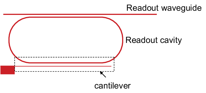
It is convenient to adopt the interaction picture with respect to , i.e., to move to the frame rotating at the pulse central frequency . In this frame, the master equation becomes
| (3) |
with
| (4) |
where is the cavity detuning, and we have defined , a dimensionless position operator of the mechanical resonator.
Due to the assumption , it is possible to neglect the effect of the free mechanical Hamiltonian in Eq. (4) during the first pulse, so that the dynamics become easy to solve. In this limit, in fact, the resonator position is a constant of motion, and it is therefore convenient to work in the position eigenstate basis, . To be more specific, assuming a factorized initial state , and writing the initial state of the mechanical resonator in the position eigenstate basis as , the state of the whole system at the end of the first pulse can be written as
| (5) |
where is the time evolution superoperator acting only on the cavity mode and where and are real valued parameters. This time evolution is simple and describes a driven cavity mode, with decay rate and detuning . In the present case, the initial state is given by a thermal equilibrium state at temperature , for the mechanical resonator, and by the vacuum state for the cavity mode. The dynamics determined by the superoperator preserves coherent states, that is, transforms an initial coherent state into another coherent state, and it is easy to verify that
| (6) |
where is the coherent state of mode with amplitude
Since we have assumed , one can well approximate the amplitude at the end of the first pulse with its asymptotic value,
| (7) |
Therefore the state of the optomechanical system at the end of the first pulse can be written as
| (8) |
where
| (9) |
is the coordinate representation of the thermal equilibrium state of the mechanical oscillator [26], with mean thermal vibrational number . Since we want to test the sensitivity of the optomechanical device at single-photon level, we assume a very weak resonant driving pulse, that is we choose , and a mean number of cavity photons at the end of the pulse, .
After the first pulse, cavity mode quickly decays to the vacuum state in a time roughly equal to , with a negligible effect on the motion of the mechanical resonator, whose reduced state at the end of the first pulse is obtained by tracing out mode in Eq. (8),
| (10) | |||||
where
is the overlap between the two coherent states. Using Eqs. (7) and (9) and exploiting the fact that , one has that the state of the mechanical resonator at the end of the first pulse is equal to
| (11) |
Due to the assumptions above, the optomechanical interaction during the first pulse does not change the probability distribution of the oscillator position . This interaction however changes the momentum distribution of the oscillator, as manifested by the modification of the off-diagonal terms () of the density matrix of the mechanical oscillator. This modification is more evident if we represent such a state in the phase space picture provided by the Wigner function, which is related to the position representation of the density matrix by the following Fourier transform [27]
| (12) |
If we insert Eq. (11) into this definition we get a non Gaussian integral, which will be approximately evaluated in the following section.
II.2 Second step: free dynamics between the two pulses
The adoption of the Wigner function is useful also because the dynamics during the second step of the experiment is easier to describe in this picture. During this step, which lasts a time interval , the cavity remains empty because mode is back in its vacuum state and no other mode is excited. Therefore, only the mechanical resonator evolves, driven solely by its free Hamiltonian , because we have assumed , implying that dissipative effects are negligible as long as . The corresponding time evolution in the Wigner representation is simply a rotation in phase space by an angle . In fact, denoting with the Wigner function associated with the state of the resonator at the end of the first pulse of Eq. (11), and with the Wigner function at time , just before the second pulse, one has
| (13) | |||
The state of the resonator just before the second pulse can be equivalently written in the position representation by taking the inverse Fourier transform of Eq. (12), getting
| (14) |
II.3 Third step: the second probe pulse is sent into the cavity and its intensity is detected
The second pulse is quasi-resonant with a second, different mode, of the cavity, with annihilation operator . However we assume again the bad cavity limit of unresolved sidebands and we again choose a pulse duration such that and . Therefore the dynamics is identical to that taking place during the first pulse, with index replaced by index , associated with the second probe mode. In the interaction picture with respect to , i.e., in the frame rotating at the pulse central frequency the dynamics of the density operator of the system formed by cavity mode 2 and by the mechanical resonator is now generated by the master equation
| (15) |
where
| (16) |
where is the detuning of the second cavity mode. The parameters associated with this second mode, , , , and the duration of the second pulse are generally different from those associated with the first mode, but their order of magnitude is just the same (apart from which is now much larger because the probe pulse is more intense than the first). In particular, since the initial state of mode 2 is again the vacuum state , one can repeat exactly the same calculation and approximations made in step 1. This means that the oscillator does not move during the second pulse and that also mode is always in a coherent state. Therefore, the state of the system formed by the cavity mode 2 and the mechanical beam, at the end of the second pulse, can be written as
| (17) |
where is just the state in the position representation of Eq. (14), and is the coherent state of mode with amplitude
The measured observable is the number of photons in mode , which, using the final state of Eq. (17) and Eq. (14), can be written as
| (18) | |||||
This expression has an intuitive explanation since it shows that the intensity of the second pulse is given by the usual Lorenzian response of the cavity, with a detuning modulated by the resonator motion, averaged over the pertinent phase-space distribution of the mechanical resonator. Eq. (18) also illustrates the basic idea of the proposed experiment: in fact, the detection of oscillations of as a function of with period equal to would be an evident signature of the effect of the force imparted by the single-photon pulse. In fact, the resonator position will oscillate at angular frequency , consequently modulating the detuning and the intracavity photon number. The average over the phase-space distribution of the mechanical resonator implies that the “fringe” visibility of these oscillations may be blurred by thermal effects. We expect in fact that the time modulation of the signal (i.e., of the intracavity photon number) is visible only if the momentum kick provided by the first single-photon pulse emerges from the average over the thermal distribution, and this is possible only if the single-photon optomechanical coupling is large enough.
Eq. (18) can be explicitly calculated in terms of the system parameters, by first changing integration variables and explicitly writing in terms of the position representation of the resonator state after the first pulse of Eq. (11). Using and , one finally gets
| (19) |
where is explicitly given by by Eq. (11),
| (20) |
Eqs. (19)-(20) can be evaluated numerically and provide the desired signal under the only assumptions and , . An explicit example is shown in Fig. 2, which corresponds to the parameter set illustrated in the figure caption. The time modulation of the intensity of the second pulse is rather weak, with a fringe visibility of the order of , which however should be visible by acquiring sufficiently large statistics.

III Analysis of the results
The dependence of the visibility upon the various system parameters, and the conditions under which the signal modulation due to the resonator motion caused by the first single-photon kick can be better understood by approximately evaluating the general expressions of Eqs. (19)-(20). In fact, one can derive a much simpler expression for in the limit of not too strong single-photon coupling, . This condition is quite easily satisfied and in fact, the parameters of Fig. 2 correspond to . This assumption allows to simplify the expression of the exponent in Eq. (11). In fact, at second order in we get
| (21) |
As a consequence, in this limit, using the definition of Eq. (12), the Wigner function of the resonator at the end of the first pulse can be easily evaluated, and one gets
| (22) |
where
| (23) | |||||
| (24) |
Eq. (22) shows that, due to the kick exerted by the first pulse, the mechanical beam acquires a nonzero mean momentum . At second order in one has also an increase of the width of the momentum probability distribution with respect to the thermal width (see Eq. (24)). However this correction is negligible with respect to the thermal width even at zero temperature , because in the experimental regime we are considering and . Therefore a first order treatment in is well justified and we shall assume from now on. This implies that at the end of the first pulse the state of the mechanical resonator is, with a good approximation, equal to a thermal state displaced along the momentum axis by the nonzero mean momentum .
Then, using the fact that between the two pulses one has the free oscillation of the mechanical resonator which is a rotation by an angle in phase space, and taking the inverse Fourier transform, one gets for the position representation of the state of the mechanical resonator before the second pulse
| (25) |
The probability distribution of the resonator position just before the second pulse is immediately obtained putting in Eq. (25): as expected, the momentum kick received by the mechanical resonator during the first pulse manifests itself as an oscillation with frequency of the center of the probability distribution. However, due to the condition this probability distribution of the resonator position is still valid at the end of the second pulse, and therefore inserting it in the general equation for the detected signal of Eq. (18), one gets
| (26) |
which is much simpler than the general expression of Eq. (19) obtained without assuming also . Changing integration variable we can also rewrite it as
| (27) |
where we have introduced an effective time-dependent detuning
| (28) |
This simpler expression for the intensity of the probe pulse is the convolution of a Gaussian probability distribution (which comes from the thermal distribution of the oscillator position) with the Lorenzian curve associated with the cavity mode response. This convolution is the well-known Voigt profile function in spectroscopy.
From this expression one can estimate how the fringe visibility is influenced by the various system parameters. The Voigt function is well approximated by a Lorenzian or by a Gaussian depending upon the ratio between the width of the two curves. If the Gaussian width (given by the thermal equilibrium width ) is much larger than the Lorenzian width (given by ) then Eq. (27) is well approximated by a Gaussian, because one can replace the Lorenzian with a suitably normalized Dirac delta function. In the opposite case the role of the Gaussian and Lorenzian curves are exchanged. When , the Gaussian distribution is wider and we can approximate
| (29) |
This equation reproduces the correct “classical” limit, which we mean as the limit of very large temperatures and at the same time very large intensity of the second driving pulse, i.e., and , but with constant. In such a limit the detected probe intensity becomes a constant and does not oscillate, that is, the fringe visibility is equal to zero. An explicit expression of the fringe visibility can be obtained in this limit, using Eq. (28) for : one gets
| (30) | |||
Fig. 2 refers to a set of parameters in which we can approximately apply the present Gaussian approximation of the Voigt function. In fact, we have chosen in Fig. 2 and , and in fact Eq. (30) gives as found in Fig. 2.
It is interesting to study the opposite limit in which the Gaussian thermal distribution is much narrower than the Lorenzian and one can approximate the former with a Dirac delta in Eq. (27). Using also the expression of of Eq. (28), we get
| (31) |
that is, the intensity of the probe pulse is a Lorenzian modulated in time by the resonator motion caused by the kick imparted by the first pulse. In such a case the visibility is given by
| (32) |
This visibility is maximized for the following choice of the detuning,
which corresponds to the maximum fringe visibility
| (33) |
We note that the visibility predicted here, although weak, could be measured with the state-of-the-art single photon detectors. To obtain good statistics, 1 million repeated measurements need to be carried out to distinguish a visibility of . At kHz repetition rate, this corresponds to 20 minutes counting time. The dark count of the detector should be much less than 1000 during this measurement time. Recently such detector has emerged and made available in an integrated photonic circuit [28]. In fact, quantum efficiency up to 50% can be reached with dark count rate less than 0.1 Hz, or 100 counts in 20 minutes [29]. It is foreseeable that a fully integrated device system with on-chip single photon detectors would allow unambiguous determination of single photon effect.
IV Conclusions
We have proposed an interferometric scheme employing an experimentally achievable optomechanical device with sufficiently large single photon optomechanical coupling , able to detect and measure the effect of an almost instantaneous optomechanical force exerted by a single photon pulse on a nanomechanical resonator. If the single-photon optomechanical coupling and the mechanical quality factor are sufficiently large, the coherent oscillations of the resonator caused by the kick imparted by a single photon pulse could be detected as time-dependent modulations of the light intensity at the cavity output. This represent a viable scheme able to unambiguously prove optomechanical effects at the single photon level, and which could be efficiently employed also in different scenarios for the interferometric detection of weak impulsive forces in nanomechanical devices.
V Acknowledgments
This work has been supported by the European Commission (ITN-Marie Curie project cQOM and FET-Open Project iQUOEMS), by MIUR (PRIN 2011), and DARPA MTO’s ORCHID program through a grant from AFOSR.
References
- [1] J. D. Teufel, T. Donner, D. Li, J. W. Harlow, M. S. Allman, K. Cicak, A. J. Sirois, J. D. Whittaker, K. W. Lehnert, and R. W. Simmonds, Nature 475, 359 (2011).
- [2] J. Chan, T. P. M. Alegre, A. H. Safavi-Naeini, J. T. Hill, A. Krause, S. Groblacher, M. Aspelmeyer, and O. Painter, Nature 478, 89 (2011).
- [3] E. Verhagen, S. Deleglise, S. Weis, A. Schliesser, T. J. Kippenberg, Nature 482, 63 (2012).
- [4] K. Hammerer, C. Genes, D. Vitali, P. Tombesi, G. J. Milburn, C. Simon, and D. Bouwmeester, arXiv:1211.2594 (2012).
- [5] P. Rabl, Phys. Rev. Lett. 107, 063601 (2011).
- [6] A. Nunnenkamp, K. Børkje, and S. M. Girvin, Phys. Rev. Lett. 107, 063602 (2011).
- [7] X.-W. Xu, H. Wang, J. Zhang, and Y.-x. Liu, Phys. Rev. A 88, 063819 (2013).
- [8] J.-Q. Liao, H. K. Cheung and C. K. Law, Phys. Rev. A 85 025803 (2012).
- [9] X. W. Xu, Y. J. Li and Yu-xi Liu, Phys. Rev. A 87, 025803 (2013).
- [10] A. Kronwald, M. Ludwig, and F. Marquardt, Phys. Rev. A 87, 013847 (2013).
- [11] M. Ludwig, A. H. Safavi-Naeini, O. Painter, and F. Marquardt, Phys. Rev. Lett. 109, 063601 (2012).
- [12] K. Stannigel, P. Komar, S. J. M. Habraken, S. D. Bennett, M. D. Lukin, P. Zoller, and P. Rabl, Phys. Rev. Lett. 109, 013603 (2012).
- [13] B. Pepper, R. Ghobadi, E. Jeffrey, C. Simon, and D. Bouwmeester, Phys. Rev. Lett. 109, 023601 (2012).
- [14] M. R. Vanner, M. Aspelmeyer, and M. S. Kim, Phys. Rev. Lett. 110, 010504 (2013).
- [15] U. Akram, W. P. Bowen, and G. J. Milburn, New J. Phys. 15, 093007 (2013).
- [16] T. Hong, H. Yang, H. Miao, and Y. Chen, Phys. Rev. A 88, 023812 (2013).
- [17] P. Sekatski, M. Aspelmeyer, and N. Sangouard, Phys. Rev. Lett. 112, 080502 (2014).
- [18] C. Galland, N. Sangouard, N. Piro, N. Gisin, and T. J. Kippenberg, Phys. Rev. Lett. 112, 143602 (2014).
- [19] M. Eichenfield, R. Camacho, J. Chan, K. J. Vahala, and O. Painter, Nature 459, 550 (2009).
- [20] J. Chan, A. H. Safavi-Naeini, J. T. Hill, S. Meenehan, and O. Painter, Appl. Phys. Lett. 101, 081115 (2012).
- [21] M. Li, W. H. P. Pernice, C. Xiong, T. Baehr-Jones, M. Hochberg, and H. X. Tang, Nature 456, 480 (2008).
- [22] W. H. P. Pernice, M. Li, and H. X. Tang, Opt. Express 17, 1806 (2009).
- [23] H. J. Mamin, D. Rugar, Appl. Phys. Lett. 79, 3358 (2001).
- [24] B. He, Phys. Rev. A 85, 063820 (2012).
- [25] The resonator actually interacts also with all the other cavity modes with a similar interaction term. However, these modes are undriven and therefore always remain in their vacuum state. As a consequence, they have no effect on the resonator motion and can be neglected in Eq. (1).
- [26] L. D. Landau, and E. M. Lifshitz, Statistical Physics, Paragraph 3.30.
- [27] C. W. Gardiner and P. Zoller, Quantum Noise, Springer, New York, 2001.
- [28] W. P. H. Pernice, C. Schuck, O. Minaeva, M. Li, G. N. Goltsman, A. V. Sergienko, and H. X. Tang, Nat. Comm. 3, 1325 (2012).
- [29] C. Schuck, W. P. H. Pernice, H. X. Tang, Scientific Reports 3, 1436 (2013).