Influence of spatially varying pseudo-magnetic field on a 2D electron gas in graphene

In 2004, the discovery of an one atom thick material was announced, which rapidly caught the attention of many physicists [1]. Graphene, a single layer of carbon atoms in a honeycomb lattice, is considered a truly two dimensional system. The carriers within it behave as two-dimensional massless Dirac fermions [2]. Due to its peculiar physical properties, graphene has great potential for nanoelectronic applications [3, 4, 5]. Graphene can be considered a zero-gap semiconductor. This fact prevents the pinch off of charge currents in electronic devices. Quantum confinement of electrons and holes in nanoribbons [6] and quantum dots [7] can be realized in order to induce a gap. However, this lattice disorder suppresses an efficient charge transport [8, 9]. One alternative to open a gap is to induce a strain field in a graphene sheet onto appropriate substrates [10]. They play the role of an effective gauge field which yields a pseudo-magnetic field [11]. Unlike actual magnetic fields, these strain induced pseudo-magnetic fields do not violate the time reversal symmetry [12, 13].

Recently, some works devoted to the search for solutions of the Dirac equation with position dependent magnetic fields were addressed [14, 15, 16, 17]. However, they consider actual instead of pseudo-magnetic fields. No experiments have been reported yet and we believe it is because such field configurations are not easy to implement in the laboratory. In this paper, we investigate a graphene sheet in the presence of both a constant orthogonal magnetic and an orthogonal pseudo-magnetic field. We consider the pseudo-magnetic field falling as $1/x^{2}$. This configuration is not known experimentally, but in considering it as induced by elastic deformations in graphene, we believe someone would be able to implement it in the laboratory. Moreover, this is the simplest case where we can get analytical solutions. Specifically, we investigate how such non constant pseudo-magnetic field modifies the relativistic Landau levels. We will solve the squared Dirac equation and show that among the possible choices for the wavefunction, the correct is the one that diverges at the origin of the coordinate system. This is compatible with the fact that our differential equation diverges at the origin as well. In Ref. [18], it is discussed that this is the correct choice if singularity is taken into account. Otherwise, we would get the wrong spectrum. This is also in agreement with other quantum problems where singularities have also appeared. This question about the correct behavior of wavefunctions whenever we have singularities has been investigated via the self adjoint extension approach over the last years [19]. An important result is that the zero-energy, which exist in the known relativistic Landau levels when just the constant orthogonal magnetic field is present, does not show up for a specific range of the parameter characterizing the varying pseudo-magnetic field. The consequence is that a Hall plateau develops at the null filling factor (dimensionless ratio between the number of charge carriers and the flux quanta). Modifications in the relativistic cyclotron frequency are examined as well.

In this section, we will investigate how a varying pseudo-magnetic field perpendicular to a graphene sheet is going to affect the relativistic Landau levels. First, we must remember the reader that the low-energy excitations of graphene behave as massless Dirac fermions, instead of massive electrons. These low-energy excitations are described by the $(2+1)$-dimensional Dirac equation

where $\sigma=\left(\sigma_{x},\sigma_{y}\right)$ are the Pauli matrices, $\Psi=(\varphi_{1},\varphi_{2})^{T}$ is a two-component spinor field, the speed of light $c$ was replaced by the Fermi velocity ($v_{F}\approx 10^{6}$m/s) and $\hbar$ has been fixed equal to one. The electronic states around the zero energy are states belonging to distinct sublattices. This is the reason we have a two component wavefunction. Two indexes to indicate these sublattices, similar to spin indexes (up and down), must be used. The inequivalent cornes of the Brillouin zone, which are called Dirac points, are labeled as $K$ and $K^{{}^{\prime}}$ [20, 21].

In this work, the varying pseudo-magnetic field is supposed to appear due to strains on a graphene sheet [22]. The valleys $K$ and $K^{{}^{\prime}}$ feel an effective field of $\tilde{\mathbf{A}}\pm\mathbf{A}$, where $\tilde{\mathbf{A}}$ is due to a real magnetic field and $\mathbf{A}$ is due to a pseudo-magnetic field. Notice that a different sign has to be used for the gauge field due to strain at the valleys $K$ and $K^{{}^{\prime}}$ since such fields do not break time reversal symmetry [23]. Considering the Landau gauge, we have

where $\lambda$ is a constant. This way, the magnetic field is $\mathbf{B}=\left[B_{0}\pm\frac{\lambda}{x^{2}}\right]\mathbf{\hat{z}}$. The first term in this field, $B_{0}$, corresponds to a constant magnetic field along the $z$ direction which is perpendicular to the graphene plane.

Going back to the problem, we consider the electronic states around the valley $K$ and the minimal coupling for electrons as $-i\mathbf{\nabla}\longrightarrow-i\mathbf{\nabla}+e\mathbf{A}=\mathbf{\pi}$. Then,

For the valley $K^{{}^{\prime}}$ we make the change $\lambda\rightarrow-\lambda$.

The Hamiltonian is given by

Writing

and using Eq. (3), we can write Eq. (1) in the form

where

and

Taking the time derivative of Eq. (6), we are able to write the second order Dirac equations for both $\varphi_{1}$ and $\varphi_{2}$, that is

and

Considering

where $\varphi(\mathbf{r})$ is the spatial part of the spinor component $\varphi_{2}(\mathbf{r},t)$, we obtain

Equation (12) above provides

The wavefunction can be factorized as $f(x)g(y)$. Since the vector potential depends on the $x$ coordinate, only the fermions will behave as plane waves in the $y$ direction. Then, we consider the ansatz for (13) as

which yields

where

By defining the dimensionless variable

Eq. (15) reads

where

The general solution of this differential equation can be obtained by using the Frobenius method to find series expansions. A similar differential equation was obatined in Ref. [24] and it was found that

where $\beta$, $\alpha$, $\gamma$ are constants and $\mathrm{HeunB}$ is the so called biconfluent Heun function [25]. We considered the modulus in the first piece in (20) since $\chi\in\left(-\infty,\infty\right)$ [26]. By substituting Eq. (20) into Eq. (18), it results in

where $C_{1}$ and $C_{2}$ are normalization constants. In order to investigate bound states, the general wavefunction must be square-integrable:

We then analyze the asymptotic behavior of solutions to the equation above, for $\chi\rightarrow 0^{\pm}$ and $\chi\rightarrow\pm\infty$. The exponential term guarantees that

if the series $\mathrm{HeunB}$ reduces to a polynomial of degree $n$. No further condition must be considered for the wavefunction. But we must be careful in choosing the right solution since our differential equation (18) has a singularity at $\chi=0$. Considering $C_{1}\equiv 0$ in Eq. (21), we have

which means that the wavefunction is regular at the origin ($\mathrm{HeunB\rightarrow 1}$ as $\chi\rightarrow 0$ [25]). On the other hand, if we take $C_{2}\equiv 0$, the wavefunction (21) might diverge at the origin because of the term ${\left|\chi\right|}^{\left(1-\sqrt{1-4\,\mathrm{F}}\right)/2}$. This said, we conclude that the solution compatible with the fact that our differential equation is singular at $\chi=0$ must be that with $C_{2}\equiv 0$ in Eq. (21), i.e., we put $C_{1}\equiv 0$, and

Otherwise, we can get the wrong spectrum as discussed in [18]. We will see bellow that this is the only choice which recovers the known spectrum for an orthogonal constant magnetic field, $B_{0}$. Notice that a divergence in the wavefunction happens when

From this last equation, the divergence in the wavefunction exists for $e\lambda<0$ and for $e\lambda>1$.

We must investigate the behavior of quantum probability as $\chi\rightarrow 0$. When $\mathrm{HeunB}$ is a polynomial of degree $n$, we have

To avoid divergence in this equation, we must impose

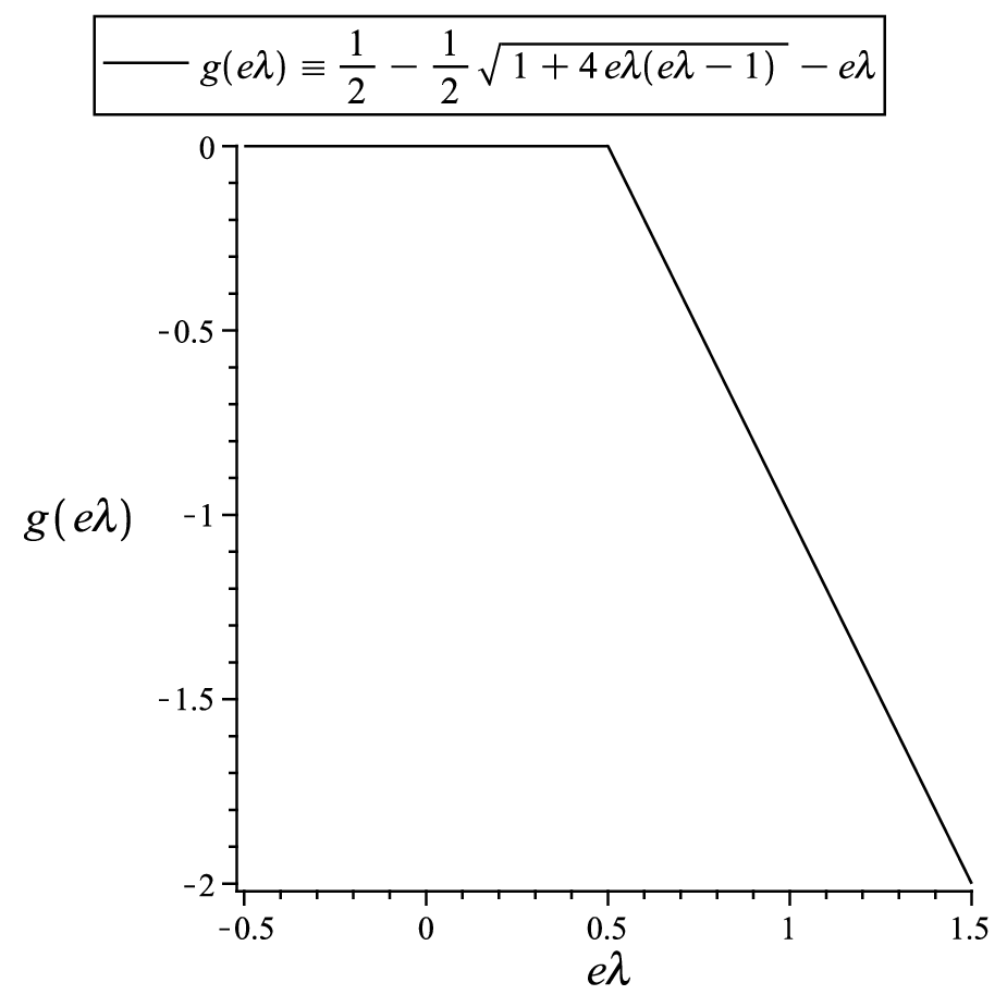
In Fig. 1, it is depicted Eq. (28). It shows that the parameter $e\lambda$ can assume any real value in the interval $(-1/2,3/2)$. This interval comes from finding the roots of Eq. (28). Before continuing, we must mention that the $1/x^{2}$ potential can lead to the "fall to the center" problem [27]. In order to prevent this phenomenon, we must have $1-4\mathrm{F}\geq 0$. This expression can be put in two forms, $(1-2e\lambda)^{2}$ and $(-1+2e\lambda)^{2}$. We conclude that physical solutions appear in the interval $(-1/2,3/2)$. For $e\lambda=1/2$, we have $1-4\mathrm{F}=0$. As we saw above, the wavefunctions diverge for $e\lambda<0$ and $e\lambda>1$. This means that regular solutions exist for $0\leq e\lambda\leq 1$ and irregular solutions exist for $-1/2<e\lambda<0$ and $1<e\lambda<3/2$.

Finally, the biconfluent Heun series becomes a polynomial of degree $n$ when [28]

with $n=0,1,2,3...$. Putting $E\equiv E_{n}^{\lambda}$ and using Eq. (19), we arrive at

Notice that, for $\lambda=0$, we get

which is the known relativistic Landau levels expression for massless fermions in the presence of a constant orthogonal magnetic field. If we had chosen the regular wavefunction in Eq. (21), we would have found $E_{n}^{0}=\pm v_{F}\sqrt{2e\left|B_{0}\right|\left(n+1\right)}$ as $\lambda\rightarrow 0$. So, this corroborates with our statement above that the correct solution must be that which may show divergence in the wavefunction at the origin.

It is useful to plot the energy versus the parameter $e\lambda$ in order to see clearly the modifications introduced by this varying pseudo-magnetic field. As it is known, there is a zero energy mode for $n=0$ in Eq. (31). In Fig. 2, we plot $(E_{0}^{\lambda})^{2}/2ev_{F}^{2}\left|B_{0}\right|$ for the $n=0$ mode. From it, we observe that the zero mode does not show up when $1/2<e\lambda<3/2$ since for $n=0$ the eigenvalues are imaginary. The zero mode still exists for $-1/2<e\lambda\leq 1/2$. We now look to the anomalous quantum Hall effect on graphene to see the consequence of this result. The Hall conductivity is generally given by $\sigma_{xy}=\nu e^{2}/h$, where $\nu$ is the filling factor (dimensionless ratio between the number of charge carries and the flux quanta), $e$ is the electrical charge and $h$ is the Planck^,s constant. At the Dirac point, both holes and electrons coexist at the zero energy and there is a finite (and quantized) contribution to the transverse conductivity given by $\pm 2e^{2}/h$. In simple words, varying the concentration of charge carries the Hall conductivity $\sigma_{xy}$ will show up as an uninterrupted ladder of equidistant steps [2, 29]. Ignoring the many-body effects, the Hall conductivity on graphene is given by $\sigma_{xy}=\pm 4e^{2}/h(n+1/2)$, where $n$ is the Landau level index and the factor 4 appears due to double valley and double spin degeneracy. This expression shows that plateaus of conductivity are formed when $\nu=\pm 4(n+1/2)=\pm 2,\pm 6,\pm 10...$. The filling factors $\nu=\pm 2$ correspond to the $n=0$ mode (zero energy). When we turn on the varying magnetic field, the zero Landau level fails to develop and the plateaus at $\nu=\pm 2$ collapse into one single plateau at $\nu=0$ [30]. Then, we have the subsequent plateaus formerly at $\nu=\pm 6$ appearing at $\nu=\pm 4$, and so on. Further analysis about the quantum Hall effect, taking into account the electron-electron interactions [31, 32, 33], should be carried out in a future work.

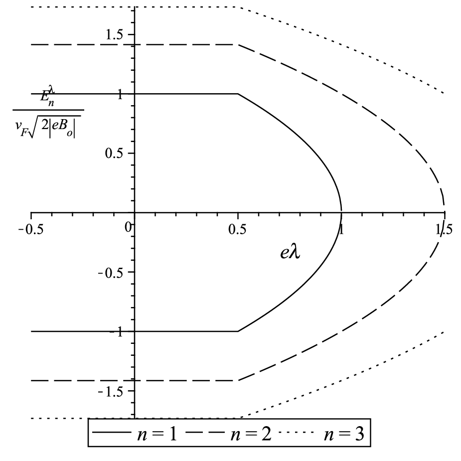
In Fig. 3, we plot the Landau levels (30) versus the parameter $e\lambda$ for $n=1,2,3$. The energies shift to lower values for positive energies (holes) and to higher values for negative energies (electrons) when $1/2<e\lambda<3/2$ (see Fig. 4).

The energy spectrum remains unchanged for $-1/2<e\lambda\leq 1/2$. Notice that the $n=1$ energy mode assumes real values only until $e\lambda=1$. These results are going to affect the relativistic cyclotron frequency as

which is depicted in Figs. 5a and 5b. From them, we see that, for $n=1$, $\omega_{c}$ increases as we raise the parameter $e\lambda$ in the interval $1/2<e\lambda\leq 1$. After $e\lambda=1$, the frequency is imaginary. For $n\geq 2$, $\omega_{c}$ increases as we raise the parameter $e\lambda$ in the interval $1/2<e\lambda<3/2$ and this effect is stronger for lower values of $n$. Then, many physical properties on graphene which depends on $\omega_{c}$ are going to be influenced by the presence of the varying magnetic field considered here. For example, it might have some impact in problems involving transitions between Landau levels induced by external radiation [34].

For the solutions around the valley $K^{{}^{\prime}}$, we just change $\lambda$ by $-\lambda$. This way, we have $-3/2<e\lambda<1/2$. For $n=0$, the zero energy is absent when $-3/2<e\lambda<1/2$. The zero energy mode exists if $-1/2\leq e\lambda<1/2$, as before. We then conclude that the pseudo-magnetic field given by $1/x^{2}$ fails to observe the zero Landau level around both valleys, $K$ and $K^{{}^{\prime}}$.

Other problems were it should be interesting to investigate the consequences of spatial modulation on the relativistic Landau levels are the relativistic version of Schrodinger cat states [35] and the study of quantum phase transitions [36].

In this work, we investigated how the relativistic Landau levels are modified if fermions on graphene are held in the presence of a constant orthogonal magnetic field together with a spatially varying orthogonal pseudo-magnetic field. We considered the latter falling as $1/x^{2}$. We were able to study this problem analytically since our squared Dirac equation yielded a differential equation called Biconfluent Heun equation, whose solution is well established and has appeared in many contexts [14, 24, 37], helping addressing different physical problems analytically as we did here. We have observed that such elastic field, given by $1/x^{2}$, fails to observe the zero Landau level around both valleys, $K$ and $K^{{}^{\prime}}$. The consequence is that a Hall plateau develops at the filling factor $\nu=0$.

We also examined the energy shift due to the presence of the varying pseudo-magnetic field and we investigated how it influences the relativistic cyclotron frequency. We saw that irregular wavefunctions and wavefunctions which do not diverge (they are regular solutions) are present. We observed that the relativistic Landau Levels are unchanged when $-1/2<e\lambda\leq 1/2$. So, since we theoretically described a way to manipulate the relativistic Landau levels, we hope our work being probed in the context of graphene, a material which has great potential for electronic applications.

As a final word, we mention that graphene under different position-dependent magnetic fields was investigated theoretically in reference [38], including the magnetic field proportional to $1/x^{2}$ alone. It would also be interesting to investigate them as pseudo-magnetic fields combined with a constant magnetic field as we did here. If either simulations or experiments involving graphene fail to observe the zero Landau level, the presence of varying pseudo-magnetic fields should be investigated. Another possibility is the presence of topological defects on a graphene sheet, since their existence also split the zero energy [39].

This work was supported by the CNPq, Brazil, Grants No. 482015/2013-6 (Universal), No. 476267/2013-7 (Universal), No. 306068/2013-3 (PQ) and FAPEMA, Brazil, Grant No. 00845/13 (Universal).

References

- [1] K. S. Novoselov, A. K. Geim, S. V. Morozov, D. Jiang, Y. Zhang, S. V. Dubonos, I. V. Grigorieva, A. A. Firsov, Science 22 October 2004: Vol. 306 no. 5696 pp. 666-669.
- [2] A. H. Castro Neto, F. Guinea, N. M. R. Peres, K. S. Novoselov and A. K. Geim, Rev. Mod. Phys. 81 (2007) 109.
- [3] Y. Sun, Q. Wu and G. Shi, Energy Environ. Sci. 4 (2011) 1113.
- [4] F. Schwierz, Nature Nanotechnology 5 (2010) 487.
- [5] J. Li, X. Cheng, A. Shashurin, M. Keidar, Graphene 1 (2012) 1-13.
- [6] F. Sol, F. Guinea and A. H. C. Neto, Phys. Rev. Lett. 99 (2007) 166803.
- [7] M. Y. Han, B.Ozyilmar, Y. Zhang and P. Kim, Phys. Rev. Lett. 98 (2007) 206805.
- [8] E. R. Mucciolo, A. H. C. Neto and C. H. Lewenkopf, Phys. Rev. B 79 (2009) 075407.
- [9] K. Nakada, M. Fujita, G. Dresselhaus and M. S. Dresselhaus, Phys. Rev. B 54 (1996) 17954.
- [10] G. Cocco, E. Cadelano and L. Colombo, Phys. Rev. B 81 (2010) 241412(R).
- [11] F. Guinea, M. I. Katsnelson and A. K. Geim, Nature Physics 6 (2010) 30-33.
- [12] F. Guinea, B. Horovitz and P. Le Doussal, Phys. Rev. B 77 (2008) 205421.
- [13] T. O. Wehling, A. V. Balatsky, A. M. Tsvelik, M. I. Katsnelson and A. I. Lichtenstein, Europhys. Lett 84 (2008) 17003.
- [14] M. R. Setare and D. Jahani, Int. Jour. of Mod. Phys. B 25 No. 3 (2011) 365.
- [15] Ş. Kuru, J. Negro and L. M. Nieto, J. Phys.: Condens. Matter 21 (2009) 455305.
- [16] R. R. Hartmann and M. E. Portnoi, Phys. Rev. A 89 (2014) 012101.
- [17] B. Roy and I. F. Herbut, Phys. Rev. B 83 (2011) 195422.
- [18] C. R. Hagen, Phys. Rev. A 77 (2008) 036101.
- [19] P. R. Giri, Phys. Rev. A 76 (2007) 012114; P. R. Giri, Mod. Phys. Lett. A 23 (2008) 2177; F. M. Andrade, E. O. Silva and M. Pereira, Phys. Rev. D 85 (2012) 041701(R); V. R. Khalilov, Eur. Phys. J. C 74 (2014) 2708; V. R. Khalilov, Theor. Math. Phys. 175 (2013) 637; V. R. Khalilov and C.-L. Ho, Ann. Phys. (N.Y.) 323 (2008) 1280; F. M. Andrade, E. O. Silva, M. Pereira, Ann. Phys. (N.Y.) 339 (2013) 510-530; F. M. Andrade and E. O. Silva, Phys. Lett. B 719 (2013) 467-471; E.O. Silva, F.M. Andrade, Europhys. Lett. 101 (2013) 51005; C. Filgueiras, E.O. Silva, F.M. Andrade, J. Math. Phys. 53 (2012) 122106; C. Filgueiras, E.O. Silva, W. Oliveira, F. Moraes, Ann. Phys. (N.Y.) 325 (2010) 2529.
- [20] S. Das Sarma, S. Adam, E.H. Hwang and E. Rossi, Rev. of Mod. Phys. 83 (2011) 407.
- [21] K. S. Novoselov, A. K. Geim, S. V. Morosov, D. Jiang, M. I. Katsnelson, I. V. Grigorieva, S. V. Dubonos and A. A. Firsov, Nature 438 (2005) 197; Y. Zhang, Y. -W. Tan, H. L. Stormer and P. Kim, Nature 438 (2005) 201.
- [22] V. M. Pereira and A. H. Castro Neto, Phys. Rev. Lett. 103 (2009) 046801.
- [23] T. Low and F. Guinea, Nano Lett. 10 (2010) 3551.
- [24] E. R. Figueiredo Medeiros, E. R. Bezerra de Mello, Eur. Phys. J. C (2012) 72 2051.
- [25] E. S. Cheb-Terrab, J. Phys. A: Math. Gen. 37 (2004) 9923.
- [26] K. Kowalski and J. Rembielński, Ann. Phys. (N.Y.) 329 (2013) 146.
- [27] A. M. Perelomov and V. S. Popov, Translated from Teoreticheskaya i Matematichskaya Fizika 4 (1970) 48.
- [28] Ronveaux, A.: Heun’s Differential Equations. Oxford University Press, Oxford (1995)
- [29] A. K. Geim and K. S. Novoselov, Nature Materials 6 (2007) 183.
- [30] A. J. M. Giesbers, L. A. Ponomarenko, K. S. Novoselov, A. K. Geim, M. I. Katsnelson, J. C. Maan and U. Zeitler, Phys. Rev. B 80 (2009) 201403(R).
- [31] F. Ortmann and S. Roche, Phys. Rev. Lett. 110 (2013) 086602.
- [32] I. F. Herbut and B. Roy, Phys. Rev. B 77 (2008) 245438.
- [33] S. Sahoo and S. Das, Indian. Jour. of Pure and App. Phys. 47 (2009) 658; S. Sahoo, Indian. Jour. of Pure and App. Phys. 49 (2011) 367.
- [34] Z. Jiang, E. A. Henriksen, L. C. Tung, Y.-J. Wang, M. E. Schwartz, M. Y. Han, P. Kim and H. L. Stormer, Phy. Rev. Lett. 98 (2007) 197403.
- [35] A. Bermudez, M. A. Martin-Delgado and E. Solano, Phys. Rev. Lett. 99 (2007) 123602.
- [36] A. Bermudez, M. A. Martin-Delgado and A.Luis, Phys. Rev. A 77 (2008) 063815.
- [37] K. Bakke, Int J Theor Phys 51 (2012) 759; M.-Aura Dariescu and C. N. Dariescu , Int. Jour. of Mod. Phys. B 27 (2013) 1350190; W. Fa-Kai, Y. Zhan-Ying, L. Chong, Y. Wen-Li and Z. Yao-Zhong, Commun. Theor. Phys. 61 (2014) 153; F. Caruso, J. Martins, V. Oguri, Ann. Phys. (N.Y.) 347 (2014) 130-140; L. B. Castro, Phys. Rev. C 86 (2012) 052201(R).
- [38] Ş. Kuru, J. Negro and L. M. Nieto, J. Phys.: Condens. Matter 21 (2009) 455305
- [39] M. J. Bueno, C. Furtado and A. M. de M. Carvalho, Eur. Phys. Jour. B 85 (2012) 53.