Phenomenological picture of fluctuations in branching random walks
Abstract
We propose a picture of the fluctuations in branching random walks, which leads to predictions for the distribution of a random variable that characterizes the position of the bulk of the particles. We also interpret the correction to the average position of the rightmost particle of a branching random walk for large times , computed by Ebert and Van Saarloos, as fluctuations on top of the mean-field approximation of this process with a Brunet-Derrida cutoff at the tip that simulates discreteness. Our analytical formulas successfully compare to numerical simulations of a particular model of branching random walk.
1 Introduction
The goal of this work is to better understand the distribution
of the particles generated by a branching random walk process
after some large evolution time.
Our initial motivation for addressing this problem comes from particle physics [1] (for a review, see [2]). In the context of the scattering of hadrons at large energies, high-occupation quantum fluctuations dominate some of the scattering cross sections currently measured for example at the LHC. These quantum fluctuations can be thought of as being built up, as the hadrons are accelerated, by the successive branchings first of their constituant quarks into quark-gluon pairs, and then of the gluons into pairs of gluons, with some diffusion in their momenta. The dynamics of these gluons is actually exactly the kind of branching diffusion process that we are going to address in this work. Therefore, results that do not depend on the detailed properties of the particular branching random walk considered may be transposed to particle physics, and give quantitative insight into hadronic scattering cross sections.
Of course, the applications of branching random walks
are much wider than particle physics.
Branching random walks may for example generate Cayley trees
which would represent the configuration space of directed polymers
in random media [3].
Although our discussion will be very general, for definiteness, we shall consider a simple model for a branching random walk (BRW) in continuous time and one-dimensional space , defined by two elementary processes: Each particle diffuses independently of the others with diffusion constant 1, and may split into two particles at rate 1, in such a way that the mean particle density obeys the equation
| (1) |
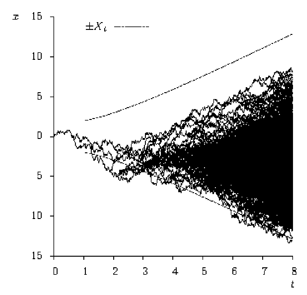
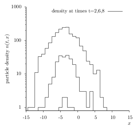
A particular realization of this BRW is represented in Fig. 1.
 |
 |
| (a) | (b) |
Several properties of BRW are known. In particular, in any given realization of the stochastic process, for large enough times, the forward part of the distribution of the particles looks like an exponential (scaled by an appropriate time-dependent constant, also depending on the particular realization considered) up to fluctuations effectively concentrated at its low-density tip. We shall call this exponential part the “front.”
Then, one can also establish rigorously [4, 5] that the probability that all particles sit at a position smaller than obeys a nonlinear partial differential equation which reads
| (2) |
This is a version of the Fisher-Kolmogorov-Petrovsky-Piscounov (FKPP) equation [6, 7]. (For an extensive review, see Ref. [8], and for more applications of the FKPP equation, see e.g. Ref. [9]). If the BRW starts at time with a single particle located at , then the initial condition is .
With such an initial condition, the solution of the FKPP equation tends to a so-called “traveling wave”. The position of a FKPP traveling wave, which is related to the average position of the rightmost particle in the BRW, is known in the large-time limit:
| (3) |
where the last term was found by Ebert and Van Saarloos [10]. (The additive constant depends on the way one defines the position of the front. It is uninteresting for our purpose.) Note that the Ebert-Van Saarloos term is a decreasing but positive contribution to the front velocity. Equation (3) may easily be extended to different branching diffusion models by appropriately replacing some numerical constants (see below, Sec. 5).
More generally, if is the number of particles at time , and is the set of their positions in a given realization, then
| (4) |
for any given function satisfies the same FKPP equation as , the initial condition being the function itself in the case of a BRW starting with one single particle at the origin. If is a monotonous function of such that and , and if reaches 1 fast enough, namely with , then the traveling wave solution holds and the front position is still given by Eq. (3). Another interesting particular case is the “critical case” when is such that exactly. Then,
| (5) |
where is a constant that we shall determine later on (see Sec. 4).
There also exists a theorem established by Lalley and Sellke
[11]
that gives the asymptotic (large time)
shape of the distribution of the position of the rightmost
particle in a frame whose origin is
at position , where is some random
variable that depends on the realization and may be thought of
as a characterization of the position of the bulk of the particles in the BRW.
(Its precise definition will be given later on).
More recently [12, 13, 14], the distribution of the
distances between the foremost particles was derived with the help of the solution to the
FKPP equation with some peculiar initial condition.
In this paper, we propose a phenomenological
picture of the fluctuations in BRW,
and we derive within this picture some new statistical properties
of a random variable similar to .
(Appendix B also lists some properties of itself.)
In Sec. 2, we shall introduce our phenomenological picture for branching random walks. Section 3 is devoted to deriving the quantitative predictions of this model for a particular random variable that can characterize the early-time fluctuations of the branching random walk. The computation of a few free constant parameters requires us to solve deterministic equations: This is explained in Sec. 4. Numerical checks are in order since our analytical results are based on conjectures: This is done in Sec. 5. In light of our phenomenological model, we shall then come back to the discussion of the Ebert-Van Saarloos result on the correction to the position of FKPP fronts (Sec. 6). Conclusions are given in Sec. 7.
2 Phenomenological description of branching random walks
2.1 Picture
The picture of the fluctuations in branching random walks (BRWs) that we have in mind is the following. There are essentially three types of fluctuations that may affect the position of the front or of the foremost particle.
- 1.
First, there are fluctuations occurring at very early times (), when the system consists in a few particles. They have a large (of order 1) and lasting impact on the position of the front or of the rightmost particle. The main effect is given by the random waiting time of the first particle before it splits into two particles, during which it diffuses, but the subsequent waiting times of the latter two particles also contribute, etc… until the system contains a large enough number of particles that makes it partly “deterministic”. We do not believe that there is a simple way to compute the effect of these fluctuations, since there is no large parameter in the problem which would allow for sensible approximations.
- 2.
Once the system contains many particles, which happens say at time , it enters a “mean-field” regime: In a first approximation, its particle density obeys a deterministic evolution with a moving absorptive boundary at a position that we shall call (and symmetrically at ), set in such a way that the particle density is 1 at some fixed distance of order 1 to the left or to the right of this boundary, respectively. These boundaries simulate the discreteness of the particles. This is the Brunet-Derrida cutoff [15], and it was shown to correctly represent the leading effect of the noise on the position of the front in the context of the stochastic FKPP equation.
From now on, we shall focus on the right boundary. (The right and the left halves of the BRW essentially decouple once the system has grown large enough). The large-time expression of the shape of the particle density near the right boundary reads, in such a model
(6) in the region , where
(7) is, up to an uninteresting non-universal additive constant, the position of the tip of the front, namely of the right boundary. The Heaviside step function enforces the fact that the particle density is 0 to the right of . , and are constants undetermined at this stage. is essentially a decreasing exponential supplemented with a Gaussian and a linear prefactors. The -dependence enters explicitly as the width of the Gaussian, and implicitly through the position of the absorptive boundary. (There are corrections to the shape of the front at order , namely to the function itself, but it turns out that we do not need to take them into account in our model, except for the determination of one overall numerical constant: We will come back to the derivation of Eq. (6) and of its corrections in Sec. 4.)
The fluctuations on top of this essentially deterministic front we have just described must take place in the tip region, where the particle density is low. We shall assume that a single fluctuation effectively gives the dominant correction to the deterministic evolution, and that the distribution of the position of this fluctuation with respect to the tip of the front is exponential:
(8) We have found (see below) that these fluctuations bring a contribution of order to the average position both of the front and of the rightmost particle in the BRW.
- 3.
Finally, there are tip fluctuations occurring at very late times, say between and , where is of order 1. They are also distributed as . They obviously add noise to the position of the tip of the front, but they do not have an effect on the bulk of the particle distribution since they do not have time to develop their own front at time .
This picture is parallel to the phenomenological model for front fluctuations proposed in Ref. [16] in the context of the stochastic FKPP problem.
2.2 Variables
To arrive at quantitative predictions for the behavior of the BRW, we need to introduce random variables that characterize the realizations. We shall discuss the following ones:
- •
, the position of the rightmost particle,
- •
, where the sum goes over all the particles in the system,
- •
.
Throughout, we shall denote by the statistical
average (over realizations) of a given variable
in the full stochastic model,
and by the value of this variable
in a mean-field approximation of the same model with a discreteness
cutoff at the tip.
(These notations have already been used in Eq. (1)
and Eqs. (6), (7) respectively.)
Discrete sums over the particles will often
be replaced by integrals wherever the particle density is large enough.
Let us briefly comment on the random variables we have just introduced.
- •
As already mentioned, is related to the solution of the FKPP equation with the step function as an initial condition.
- •
The average tends to a constant at large . In addition, in any given event, the random variable itself tends to a constant, which has some distribution (which we do not know how to compute) which may be used to characterize the early-time fluctuations. Note that an appropriate generating function of the moments of
(9) also obeys the FKPP equation, but with the “critical” initial condition discussed in the Introduction. We will come back to the latter fact in Sec. 4. Also, in the context of directed polymers in random media, is the partition function and the free energy averaged over the disorder [3].
- •
is the variable used by Lalley and Sellke in the theorem alluded to in the Introduction. However, we are not going to focus on this variable in the body of this paper, since we found it has many drawbacks for our purpose. First, a practical drawback: Although tends almost surely to a positive constant when [11], it takes negative values at finite times, with finite probability; is then undefined in these particular realizations. Second, a theoretical drawback: It turns out that the finite-time corrections to the moments of are very sensitive to the initial fluctuations, the ones that are not computable analytically. We shall nevertheless quote a few results on the distribution of in Appendix B.
In some intuitive sense, and characterize the
position of the “front” of a particular realization of the evolution at time .
The variables and keep the memory of the initial fluctuations. Therefore, we shall not attempt to compute the distribution of the fluctuations in accumulated over the whole history of the BRW, but instead the fluctuations of this variable between two large times and , in order to have a quantity that is independent of the very early times at which there is no mean-field regime.
3 Statistics of in the phenomenological picture
Here, starting from the phenomenological model defined in Sec. 2, we shall deduce new results on the distribution of the variable (and on its moments) for , up to one single constant for the moments of order larger than 2, and up to an additional constant for the first moment. Throughout, we shall aim at the accuracy for and neglect higher powers of these expansion variables.
3.1 Effect of a fluctuation on
We first compute , namely the variable in the mean-field approximation with the cutoff in the tail. Using the definition of the variable in Sec. 2.2 and using Eqs. (6),(7), we find
| (10) |
at first order in . is a constant literally equal to in this calculation, but there would also be other contributions to that we cannot get from the large- asymptotic shape of the front exhibited in Eq. (6). We shall postpone the full calculation of to Sec. 4.
It turns out that the term of order in Eq. (10) generates contributions to the distributions and to the moments that we shall address. Hence it is enough for our purpose to keep no more than the constant term, namely we write
| (11) |
We perform a more complete calculation in Appendix A, keeping the subleading terms, in order to demonstrate that this a priori approximation is indeed accurate enough.
Let us consider a fluctuation occurring at time at a distance from the tip of the deterministic front. From Eq. (7), at time such that , this fluctuation has developed its own front whose tip sits at position
| (12) |
There would of course be terms proportional to , and also here, but we again anticipate that they would eventually lead to corrections of higher order to the quantities of interest. We refer the reader to Appendix A for the details.
The shape of the front generated by this fluctuation will eventually have the form , where is a constant that we cannot determine since it is related to some “average” shape of the fluctuation. With this extra fluctuation, has the following expression:
| (13) |
The first term is just : We replace it by Eq. (11). The second term is integrated in the same way as the first one, using the expression (12) for . We find
| (14) |
Thus the forward shift in induced at time by such a fluctuation occurring at time reads
| (15) |
Note that in the asymptotic limit of interest, at first glance, the nontrivial term in this expression seems to be of order , thus, if , it is smaller than our accuracy goal. However, it is enhanced by the factor, which turns out to be large.
3.2 Probability distribution and moments
We may convert the conjectured probability of a forward fluctuation of size (Eq. (8)) into the probability distribution of the difference of between two times and by simple changes of variables. We first discuss the variable
| (16) |
The fundamental observation is that a fluctuation may essentially have
two opposite effects on
.
If it occurs after time , then it gives a positive contribution.
If instead it occurs before , it generates a negative .
Now we observe that the difference between and reads
, which is of order and
thus, we may trade for (see Appendix A
for more details).
Let us first address the case in which the fluctuation occurs between and . Using Eq. (15) together with the distribution (8), the probability that the size of the shift in induced by a fluctuation at time is less than some reads
| (17) |
We shall always assume that is finite, and the ordering . The probability distribution of then reads
| (18) |
The rate of the fluctuations is assumed constant in time, thus the distribution of results from a simple integration over from to with uniform measure. It reads
| (19) |
Exactly in the same way, we may compute the probability distribution of when the fluctuation occurs at a time smaller than . In this case, the effect on of a fluctuation of size reads
| (20) |
Using the same method, we find
| (21) |
The integral over which has to be performed to arrive at these expressions is dominated by values of of the order of . This helps us to understand a posteriori why we were allowed to drop terms of order and in Eqs. (10) and (12), respectively, although we were aiming at such accuracy for .
The probability distribution given in Eq. (19) and (21)
cannot be normalized and the first moment is also divergent. We
shall compute the latter separately in the next section.
An analytic continuation of the generating function for the moments of can be obtained from Eq. (19) and (21) by a direct calculation. We get
| (22) |
keeping in mind that this formula can be used only for moments of second order or higher.
The analytical structure of Eq. (22) is particularly
simple. There are poles on the positive real -axis, fully
contained in the first
term : They correspond to positive values of .
All the other poles, contained in the remaining terms, are located
on the real negative axis, and correspond to negative
values of .
A comment is in order on the conjectured probability distribution (8) of the tip fluctuations that we used in the above derivation. Actually, we omitted a time-dependent Gaussian factor of the form , which would cut off the exponential distribution of at a distance ahead of the tip of the front, and thus modify the distribution of for large positive . However, numerically, we do not find evidence for such a modification: It seems that Eq. (19) has a more general validity. We do not have a good explanation for this surprising fact in the context of our phenomenological model for fluctuations. But it turns out that a different calculation of the positive fluctuations outlined in Appendix C does not have such limitations.
3.3 Correction to the first moment of due to the fluctuations
Since it is not possible to use Eq. (22) to get the first moment of ,
we shall arrive at its expression through a direct calculation.
We must take into account the expansion
(keeping terms at least as large as , , )
of the density of particles in the deterministic
limit with a discreteness cutoff, and, in addition,
the effect of the fluctuations
which intermittently speed up the evolution.
We have already guessed
that there is an contribution to the deterministic
evolution (see Eq. (10)), but a full calculation will eventually
be needed.
Here, we shall simply denote by its coefficient.
The average of over realizations has thus a mean-field contribution, and a contribution from the fluctuations which in turn can be decomposed in positive and negative contributions and respectively. We shall evaluate the latter in this section.
We write
| (23) |
Using Eq. (8) and Eq. (15), we get the expression
| (24) |
for the positive part of the contribution at of the fluctuations, and
| (25) |
subtracts the effect at of the fluctuations occurring at . We have introduced a time of order 1 as a lower bound in these integrals in order to make these expressions finite. The physical meaning of this cutoff is clear: Before , there is no mean-field regime because the whole system consists in a few particles only.
Let us start with the computation of . It is useful to perform the change of variables
| (26) |
which leads to the following expression of :
| (27) |
where . is large compared to 1, except when is of order . But the contribution of the region in the -integration is smaller than , and hence negligible. So we may always assume .
The integral over is performed analytically, and the large- limit may eventually be taken:
| (28) |
The remainder reads
| (29) |
where
| (30) |
and can be performed with the help of the change of variable :
| (31) |
while for , a further integration by parts is needed to get rid of the log. We eventually arrive at the following exact expression for (29):
| (32) |
The term is the same as the term except for the replacement .
Since we are neglecting terms of relative order , and higher, we may expand the expressions for and . The difference then reads
| (33) |
Equation (23) eventually leads to the following expression for :
| (34) |
We note a very important property of this result: It does not depend on . If it did, then we would loose predictivity because is the arbitrary time after which we declare that the fluctuations are small enough for our calculation to apply. (This would not be true at the next order in , ).
4 Deterministic calculations
In this section, we first review the Ebert-Van Saarloos method [10] to compute the order correction to the mean position of the rightmost particle in the BRW . We extend the method to the position of the right boundary in the deterministic model with discreteness cutoffs , and eventually adapt it to .
The calculations presented here will enable us to determine the remaining unknown constants, namely (see Eq. (7)), (Eq. (10)), and . The latter two constants appear in particular in Eqs. (19), (21), (22) and (34).
4.1 Ebert-Van Saarloos calculation and its extension
The original calculation of Ebert and Van Saarloos aimed at finding properties of the solutions to the FKPP equation
| (35) |
for , with a steep enough initial condition, e.g. . This equation is actually the same as Eq. (2), with the correspondence . The nonlinearity can essentially be viewed as a moving absorptive boundary on a linear partial differential equation, the position of the boundary being set in such a way that has a maximum at a fixed height.
To determine the value of the constants and , we need to address a branching diffusion equation with a nonlinearity that forces to go to zero over a distance of order 1 at the right of the point at which , and which therefore acts as a tip cutoff. In terms of a smooth equation, we may write, for example,
| (36) |
and study the properties of the solutions to this equation in the region .
In both cases, the equation can be linearized in the respective domain of interest, and one gets
| (37) |
We shall assume that the nonlinear term is equivalent to a right-moving absorptive boundary at the accuracy at which we want to address the problem. (This assumption was better motivated by Ebert and Van Saarloos in their discussion of what they call the “interior expansion” [10]). In the first case, we study the function to the right of the boundary; in the second case, we study the function to the left.
Solution to the linearized equation with an appropriate boundary condition.
Near the boundary, at large times, the function reads
| (38) |
where and this is valid for . According to Ebert-Van Saarloos [10], the large- corrections to this shape are of the form (there is no term of order ). All these features should not depend on whether we address Eq. (35) or Eq. (36) above, except for the signs of and .
We write
| (39) |
where , and the following ansatz are taken:
| (40) |
The variable may be positive in the linear domain (it is the case for the usual Ebert-Van Saarloos solution) or negative: Therefore, we write , where . The ansatz for the front position contained in already incorporates the two known [5] dominant terms at large , namely . The term was new in Ref. [10].
Thanks to these ansatz, the original equation splits into a hierarchy of equations for the functions . The first two equations of this set read
| (41) |
The first equation of the hierarchy is the Kummer equation
| (42) |
with , and . Two independent solutions are, for example, the two Kummer functions (or hypergeometric functions)
| (43) |
namely, in our case,
| (44) |
The latter is just the elementary function , while the former diverges like for large , and has thus to be discarded. Hence the solution reads
| (45) |
where is a constant, arbitrary at this stage.
As for the second equation in Eq. (41) whose solution is the function , it is an inhomogeneous Kummer differential equation. A basis for the solutions of the homogeneous part is, for example, the set of the two functions
| (46) |
We need to find a particular solution of the full equation. We define ; The equation for then reads
| (47) |
and we may look for solutions in terms of a series:
| (48) |
Inserting this expression into the differential equation (47), we get the following relations between the coefficients of the series:
| (49) |
The free parameters are and . We may choose them in such a way that : We therefore set and . Then
| (50) |
where we used the duplication formula . Switching back to the variable , the final expression for the particular solution reads
| (51) |
which, except for the sign factors , is the Ebert-Van Saarloos result [10]. Following again Ref. [10], we write the solution for as
| (52) |
and inserting (52) together with (45) into (40),(38), we would get the expression of up to the constants . We are now going to determine them from a matching procedure.
Matching conditions.
We now match with the shape of the so-called “interior” region at . This means that just obtained should have the same small- expansion as the limiting form of in Eq. (38). Hence we need to impose
| (53) |
The first constraint is solved by setting . As for the second one, it means in particular that there should be no term proportional to in . This requirement leads to the equations
| (54) |
Now we must also check the behavior at . We need the expansion of the functions and for . Let us start with . We shall use the integral representation
| (55) |
We change the variable for to in the integral, and we expand the factor near :
| (56) |
We then notice that we may extend the integral to without adding exponentially-enhanced terms. Finally, we perform the remaining integration over . The result reads
| (57) |
Setting and , we write
| (58) |
We now turn to . We write the following integral representation:
| (59) |
This representation may be checked by expanding the exponential in the integral and performing the integration over . For large , the two rightmost terms do not play any role since they are not exponentially enhanced. We may now treat the first term exactly in the same way as in the case of the Kummer function . After taking the limit, which is finite once all non-exponentially enhanced terms have been discarded, we get
| (60) |
Up to an overall constant, all terms are identical to the ones in the expansion of the function.
Requiring the cancellation of these exponentially-enhanced terms in the expression (52) for leads to the equation
| (61) |
Using this equation and the second equation in (54), one determines the value of :
| (62) |
Hence this constant is positive for the Ebert-Van Saarloos solution of the FKPP equation, but is negative when one computes the position of the tip of a front with a discretness cutoff.
Matched solution.
All in all, we get
| (63) |
with
| (64) |
The first two terms in , namely , give back Eq. (6). The next terms are finite-time corrections.
Identifying with and setting , we recover the value of
| (65) |
already derived by Ebert and Van Saarloos (see Eq. (3)). With and , we read off this formula the value of the constant
| (66) |
We can also deduce the value of by using the definition of the variable given in Sec. 2.2 and the shape of the mean-field particle distribution (63):
| (67) |
which, after replacement by the expression (63) and setting , becomes
| (68) |
The term proportional to is zero after the integration, and the other terms give numerical constants. We finally find, at order ,
| (69) |
4.2 Solution of the deterministic FKPP equation with the critical initial condition
Let us consider a generating function of the moments of the variable:
| (70) |
Defining , has exactly the form shown in Eq. (4) and thus solves the FKPP equation (35), . If the initial condition for the underlying branching random walk is a single particle at position ,
| (71) |
and then, the position of the FKPP traveling wave is given by Eq. (5). In this section, we shall address this case using the Ebert-Van Saarloos method in order to obtain the correction to the latter and some analytic features of . Indeed, from the expression of , we may in principle compute the moments of , using the identity
| (72) |
General solution of the linearized equation in a moving frame.
Following Ebert-Van Saarloos, we define
| (73) |
The linearized FKPP equation for reads
| (74) |
Next, we take the ansatz , and introduce the variable . The function is expressed with the help of , and we look for solutions in the form
| (75) |
We are led to the following hierarchical set of equations (compare to Eq. (41)):
| (76) |
The solution reads
| (77) |
where are the error functions defined by
| (78) |
and are integration constants to be determined. The terms in the first square brackets in Eq. (77) correspond to the general solution of the homogeneous equation for , while the next two terms represent a particular solution of the full equation as can easily be checked.
Matching conditions.
Because of the initial condition, the tail of the front at has the exact shape
| (79) |
at any time. In particular, there is no overall constant. Comparing to Eqs. (73),(75), this condition means that
| (80) |
Let us expand our solution (77) for for large :
| (81) |
The identification with the expected asymptotic form leads to the conditions:
| (82) |
The second condition is trivial once the first one is satisfied.
We also impose that all terms that are not exponentially suppressed cancel, which is realized by setting
| (83) |
We turn to the limit . The condition (38) reads, in terms of the -function
| (84) |
which in particular forbids constant terms and terms proportional to . Since the small- expansion of our solution reads
| (85) |
we see that needs to be set to 0 and .
Putting everything together, we find that all constraints are solved by the choice
| (86) |
Note that the coefficient in Eq. (84) is determined to be , while in the noncritical case, it is a free parameter.
Matched solution.
All in all, our solution reads
| (87) |
with
| (88) |
The term is identical to the one in the “pushed front” calculation of Ref. [10], see Appendix G, Eq. (G18) therein, although the front solution chosen in that work is different, see Eq. (G7).
We can now deduce from this calculation the average value of by expanding the exact formula Eq. (72) in powers of and keeping the coefficient of the term of order :
| (89) |
We find
| (90) |
Identifying the latter equation to Eq. (34) and taking into account the value of already computed in Eq. (69), we finally obtain a determination of :
| (91) |
5 Complete results and numerical checks
Since the new results we have obtained rely in an essential way on a model for fluctuations and hence on a set of conjectures, we need to check them with the help of numerical simulations in order to get confidence in the validity of our picture. In the first part of this section, we shall list the formulas we have obtained but extending them to more general BRW models. Then, we define a model that is convenient for numerical implementation in Sec. 5.2, and we test our results against numerical simulations of this particular model in Secs. 5.3 and 5.4.
5.1 Parameter-free predictions for a general branching diffusion
We now extend our results to general branching diffusion kernels. In the continuous case, we write the equation for the average particle density as
| (92) |
where is the operator that represents the branching diffusion. The eigenfunctions are the exponential functions , and the corresponding eigenvalues are . In the case discussed in the previous sections, and . We introduce which solves . Then in the case studied so far, and .
We can also address the discrete time and space case, which is useful in particular for numerical simulations. We write
| (93) |
where now is some finite difference operator, such as
| (94) |
In this case, and take their values on lattices of respective spacing and . Again, the eigenfunctions of the kernel are the exponential functions.
The generalization of our previous results to an arbitrary BRW relies on the fact that at large times, the “wave number” dominates and the kernel eigenvalue may be expanded to second order around [8]. We then essentially use dimensional analysis to put in the appropriate process-dependent factors. We list here the generalized expressions without detailed justifications.
With the general kernel, the FKPP front position reads (see Eq. (3))
| (95) |
The position of the tip of the front in the mean-field model with a discreteness cutoff reads instead
| (96) |
This expression generalizes Eq. (7) with computed in Sec. 4.1 (see Eq. (66)).
The relevant variable that characterizes the fluctuations of the position of the bulk of the particles is . We have computed its value in the deterministic model with a tip cutoff:
| (97) |
This equation generalizes Eq. (69).
The stochasticity that we found tractable analytically is related to the fluctuations of the difference of this variable at two distinct large times and :
| (98) |
Its first moment reads
| (99) |
The probability distribution of the fluctuations reads
| (100) |
This formula is the generalized form of Eqs. (19) and (21). A generating function of the moments of order larger than 2 can be written as
| (101) |
For example, expanding this generating function, we find that the moments of order read
| (102) |
where the ’s are numerical constants. The first ones read
| (103) |
or in numbers, , , .
5.2 Model suitable for a numerical implementation
For simplicity of the implementation, we considered a discretized branching diffusion model. At each time step, a particle on lattice site (with lattice spacing ) has the probability to give birth to another particle on the same site, to move to the site , to move to the site , and to stay unchanged at the same site. The eigenfunctions of the corresponding diffusion kernel are the exponential functions , and the eigenvalues read
| (104) |
The discretization in time is chosen to be . The relevant parameters for this model are
| (105) |
5.3 Check of the deterministic analytical results
We solve the equivalent of the deterministic FKPP equation with the critical initial condition. For our discretized model, the FKPP equation becomes the finite difference equation
| (106) |
with the initial condition . Here is an integer that labels the sites of the lattice. is the logarithm of the equivalent of defined in Sec. 4. The use of a logarithmic variable avoids problems with numerical accuracy in the region , upon which the solution depends crucially.
First, we integrate the solution according to Eq. (89) in order to get . The analytical expectation for the model which is implemented is given in Eq. (99) with the numerical inputs (105):
| (107) |
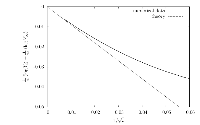
The numerical calculation is shown in Fig. 2, and is in perfect agreement with the analytical formula. In order to estimate more quantitatively the quality of this agreement, we fit a function of the form
| (108) |
where the ’s are the free parameters. The value of which we get from the fit is , which is very close to the expected value from our analytical calculation.
Next, we solve the deterministic FKPP equation with a tip cutoff. In practice, the latter cutoff is implemented as a smooth nonlinearity, as in Eq. (36). More precisely, the equation we solve numerically is the following:
| (109) |
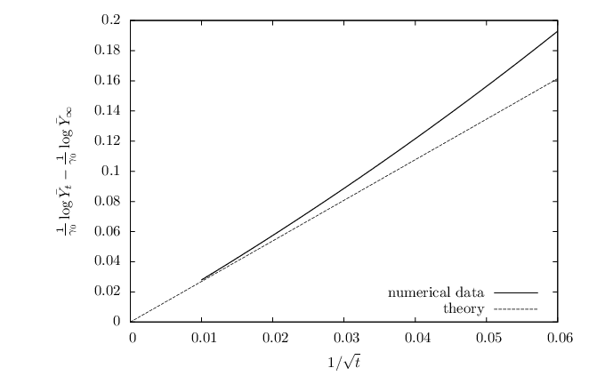
with . Here, is the logarithm of the number of particles on site at time . The logarithmic scale for the evolved function is useful here because of the exponential growth of the number of particles with time. Also in this case, the result is in excellent agreement with the analytical expectation (see Fig. 3), which, for the considered model, should read (see Eq. (97))
| (110) |
The fit of the same function as before to the numerical data gives which, again, is very close to the analytical estimate.
5.4 Check of the statistics of
We now use a Monte-Carlo implementation of the stochastic model of a branching random walk described above in order to test the probability distribution of given in Eq. (100).
The implementation is quite straightforward, except maybe that after a few timesteps, the number of particles in the central bins (typically ) becomes very large. To handle such large particle numbers, we further evolve these bins in a deterministic way. (In practice in the code, we set the limit between stochastic and deterministic evolution at .) Such an approximate treatment was tested before in a similar context, see e.g. Refs. [17, 18, 19]. As in the deterministic case discussed above, we also switch to logarithmic variables, , in order to be able to handle the large particle numbers in a standard double-precision computer representation. Of course, the low-density tails of the system are treated fully stochastically.
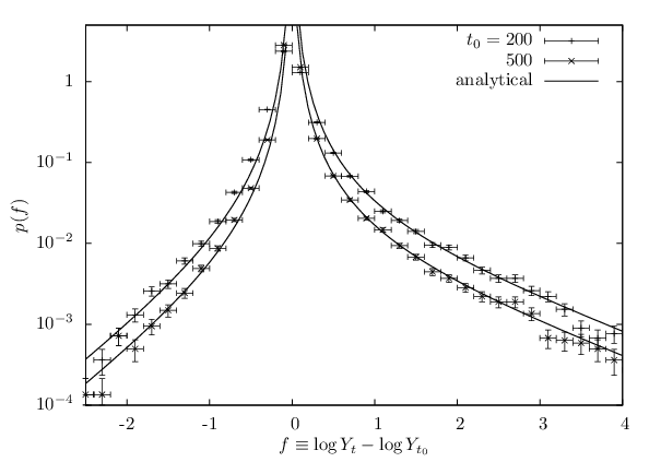
The result for the distribution of is displayed in Fig. 4 compared to the analytical formulas (100). We see an excellent agreement between the outcome of our model and the numerical data.
We can also compute numerically the first few moments of the variable and plot them against (Fig. 5).

Here again, there is a good agreement between the analytical result and the numerical calculation, although more statistics would be needed in order to reach a good accuracy for the moments of order 3 and 4.
6 Stochastic interpretation of the corrections to the position of FKPP fronts
So far, we have essentially discussed the statistics of the random variable in the light of our phenomenological picture of BRW. We are now going to address the average of the position of the rightmost particle which is also the position of the FKPP front, and whose expression at order was obtained in Ref. [10].
6.1 Correction to due to fluctuations
As in the case of , in our picture, the average value of the position of the front is given by the deterministic evolution of the bulk of the particles, supplemented by a contribution from fluctuations in the low-density region. We may write
| (111) |
In this section, we shall compute . is the contribution at time of fluctuations that occur all over the range of time and is the contribution at time of fluctuations that have occurred before :
| (112) |
where the appropriate regulators will be introduced later. is the contribution to the shift of the position of the tip of the front at time of a fluctuation of size occurring at . Let us now evaluate .
When a fluctuation occurs at time at position ahead of the tip of the regular front, then it develops its own front by independent branching diffusion. The resulting density of particles at time becomes the sum of two terms, and therefore has the shape
| (113) |
where is given by Eq. (6) and by Eq. (12). Using the latter equations, one is led to
| (114) |
The calculation of and proceeds exactly as in the case of and in Sec. 3.3. is still given by an equation of the form of (27), but with the replacements and , where now
| (115) |
Note that in the present case, late times need to be cutoff in order to ensure the convergence of the integrals: We pick some arbitrary say of order one.
The same change of variable as before may be used: , then
| (116) |
After performing the integrals and expanding in the limit of small , compared to , one gets
| (117) |
The main difference with respect to Eq. (32) (once the relevant expansions have been performed) is the presence of -dependent terms and of an extra factor 3 in the last term. As before, is deduced from the above formula by replacing by . We then see that in the difference , the and dependences cancel.
As for the moments of order , they are found to depend on , that is, on the late-time fluctuations, as they should, since is the position of the rightmost particle, which experiences a stochastic motion of size 1 over time scales of order 1.
6.2 Recovering the Ebert-Van Saarloos term
Putting everything together, namely the value of from Eq. (66) and the value of just computed, we find the interesting expression
| (118) |
The terms that grow with and are the usual deterministic terms from Bramson’s classical solution [5]. Then, the next terms, under the square brackets, are respectively the deterministic correction to the position of the discreteness cutoff in the mean-field model, and the correction due to fluctuations. We see that the latter is exactly twice the former, with a minus sign. The sum of these two terms gives back the Ebert-Van Saarloos correction for , see Eq. (3).
In other words, the mismatch between , the position of the tip of the front in the deterministic model with a cutoff, and , the mean position of the rightmost particle in the full stochastic model, is exactly due to the very fluctuations we have been analyzing in this paper.
7 Conclusions
Some time ago, we proposed a model for the fluctuations of stochastic pulled fronts [16], which are realizations of the stochastic FKPP (sFKPP) equation (for a review, see Ref. [20]). Equations in the class of the sFKPP equation may be thought of, for instance, as representing the dynamics of the particle number density in a branching-diffusion process in which there is in addition a nonlinear selection/saturation process that effectively limits the density of particles. The realizations of such equations are stochastic traveling waves. The stochasticity comes from the discreteness of the number of particles. In this context, the (deterministic) FKPP equation represents the mean-field (or infinite number of particle) limit of the full dynamics.
Expansions about the mean-field solution
were considered already a long time ago; see, e.g., Ref. [21]
where the so-called expansion (see Ref. [22])
was applied to study fluctuations in the context of
reaction-diffusion processes.
Later, we could obtain new analytical results
thanks to a phenomenological
model [16].
The picture encoded in our model was the following:
Most of the time, the traveling wave
front propagates deterministically,
obeying the ordinary deterministic
FKPP equation supplemented
with a cutoff in the tail, accounting for discreteness by making sure that
the number density of particles reaches 0 rapidly whenever it drops below 1.
Brunet and Derrida had shown [15] that such a cutoff
correctly represents the main effect of the noise on the velocity of the front.
On top of that, in our model,
there are some rare fluctuations consisting in a few particles
randomly sent far ahead of the tip of the front, which upon further evolution
build up a new front that completely takes over the old one.
A positive correction to the front velocity was found, and the cumulants of the
front position were computed (see Ref. [16]).
In the present paper, we have considered a simple branching random walk, without
any selection mechanism. We have used exactly the same ingredients as the ones
conjectured in the model for stochastic fronts, namely deterministic evolution with a cutoff
and fluctuations consisting in a few particles randomly sent ahead the
tip of the front at a distance distributed exponentially.
We were also able to
arrive at a quantitative characterization of the fluctuations of the front
in these processes.
There are however a few important differences between the branching random walk and the stochastic FKPP front. First, the initial fluctuations are never “forgotten” in the BRW case. This is because of the absence of a selection mechanism able to “kill” the front and let it be periodically regenerated by fluctuations. Therefore, we could only compute the effect of the fluctuations on the front position between two large times and . Next, while it was quite straightforward to define a proper front position in the sFKPP case (as for example the integral of the normalized particle density from position say 0 to ), it is more tricky for the simple branching random walk. We were led to consider the variables and (introduced in Sec. 2.2). Our main result is the distribution of the variable given in Eq. (100), where and are two large times such that . Interestingly enough, the distribution of the positive values of this variable is identical (up to an overall factor) to the distribution of the front fluctuations in the sFKPP case. The same holds true for the distribution of to which we dedicate Appendix B.
We were also able to discuss the average of the position of the rightmost particle, but
not its higher moments since they are sensitive to the very late-time fluctuations
which are not properly described in our model.
As for the average position,
we could nevertheless propose an appealing interpretation of the
correction to the front position computed by Ebert and Van Saarloos in Ref. [10].
There are still many open questions. Maybe the most outstanding one on the technical side would be to try and compute the statistics of (and of ) exactly, instead of relying on a phenomenological picture involving conjectures. We outlined such a calculation in Appendix C, based on the evaluation of a generating function, but without being able to complete it.
Acknowledgements
The idea at the origin of Appendix C is due to Prof. B. Derrida. We thank him also for very helpful discussions, and for his reading of the manuscript. We acknowledge support from “P2IO Excellence Laboratory”, and from the US Department of Energy, Grant No. DE-FG02-92ER40699.
Appendix A Details of the calculation of the probability distribution of
In this appendix, we go back to the calculations that lead to Eqs. (15), (19) and (21), but keeping the subleading terms that we neglected a priori in Sec. 3.1 in order to simplify the presentation.
The exact evaluation of starting from its definition given in Eq. (10), in which one inserts Eqs. (6), (7), makes use of the basic Gaussian integral
| (119) |
We immediately arrive at Eq. (10), which may also be rewritten at order as
| (120) |
We now add a fluctuation occurring say at time . It develops a front whose tip sits, at time , at position
| (121) |
which is Eq. (7) supplemented with the subleading terms. Keeping all the latter, we see that Eq. (15) just needs to be replaced by
| (122) |
As for the probability distribution of the fluctuations in Eq. (18), it becomes
| (123) |
which has to be integrated over . We recall that after integration over , the obtained expression will be correct at order , , , hence only the first nontrivial terms are relevant in the expansion of the exponential.
In the absence of terms, the integration region could be chosen to be as in Sec. 3. Now however we have a non-integrable singularity at which needs to be cut off. Hence we write
| (124) |
where is an arbitrary time interval whose length is of the order of 1.
Let us compute the integral
| (125) |
appearing in the previous expression. We expand the exponential to lowest order, and hence we get the three terms
| (126) |
where (which is essentially the same integral as in Eq. (30)) gives back the lowest-order result in Eq. (19):
| (127) |
As for the two other terms,
| (128) |
are new contributions which are subleading, as is easy to demonstrate from an exact calculation of these integrals. We start with the computation of :
| (129) |
Since , it is clear that the largest terms in are at most of order and . As for ,
| (130) |
The second term is divergent for . It gives the dominant contribution at large : . The other terms are also subleading, of order and .
Hence we see that at order , boils down to the first term in the expansion of in Eq. (127).
Lastly, we have already noticed in Sec. 3 that
| (131) |
thus replacing by in brings about only subleading contributions.
Appendix B Statistics of
In the same way as for the variable , we may try to get the statistics of from our phenomenological model. The variable is of interest since it is used in a mathematical theorem to characterize what we call the position of the front in each realization, however, as we shall see, we cannot obtain full analytical formulas for the first moment of as in the case of . Moreover, as was already commented above, the variable has properties that make it awkward for numerical simulations.
The first step is to compute in the mean-field approximation with a tip cutoff. The result reads
| (132) |
This formula is analogous to Eq. (10), but there is now a slightly stronger -dependence, , which we are able to determine completely from the leading-order shape of the particle distribution. We have dropped terms of order and higher.
The effect of a fluctuation occurring at time on is
| (133) |
(Compare to Eq. (15)). The following approximate formula can now be written for the distribution of :
| (134) |
where is given by Eq. (133), while is the probability distribution (8). The bounds on the integral over depend on whether is positive or negative. Indeed, positive values of are generated by fluctuations occurring at between and , while fluctuations before (namely between the times at which we declare that the system contains a large number of particles and ) give rise to negative values of .
The distribution of positive is quite easy to compute. It is enough to recognize that the terms of order and inside the square bracket give subleading contributions to . It turns out that the final result is very similar to (see Eq. (19)), except for the detailed form of the and dependence:
| (135) |
Inserting the value of the constant previously determined (see Eq. (91)) and going to a general branching diffusion kernel, we get
| (136) |
Negative values of are more complicated to deal with since we can no longer neglect the term in Eq. (133) a priori. Performing the change of variable and expanding for large and , the equation for simplifies to
| (137) |
Due to the Dirac -function, we see that as soon as , where solves , and hence is of order 1. This means that is of higher-order in powers of and when .
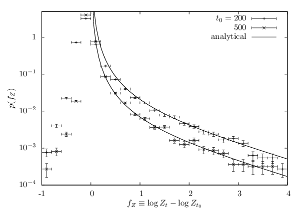
Our formula for the distribution, Eq. (136), successfully
compares to the numerical data, see Fig. 6.
We also see that the distribution of negative values of is indeed
sharply suppressed (compare to the distribution of in
Fig. 4).
As for the mean of , we found that it depends on the arbitrary time roughly as , and thus is not calculable.
Appendix C Generating function for the moments
In this section, we are going to find the form of the large positive -fluctuations from a generating function, hence from a deterministic calculation.
C.1 General framework and exact formulas
We can write the following identity:
| (138) |
see Eq. (9) for the definition of . This equation follows from the integral representation of the function, and is suitable for series expansions in , which eventually lead to the moments of . For some calculations outlined below, it will prove useful to change and to the variables
| (139) |
since Eq. (138) then holds in the very same form (just up to the replacements ) directly for the moments of .
Let us introduce the generating function
| (140) |
It is the value of this function at zero, , from which one computes the generating function in Eq. (138), which reads
| (141) |
The function may also be written as
| (142) |
where is a parameter in this equation, and
| (143) |
In this form, it is clear that obeys the FKPP equation (with time variable ), with the initial condition . But may also be written as
| (144) |
which makes it obvious that it also obeys the FKPP equation (with time variable ), with the initial condition .
So far, these formulas are exact and should in principle enable the computation of the moments of , from some hopefully limited knowledge of the properties of the solutions to the FKPP equation.
We have not been able to fully compute the generating function. However, we can use the systematic solution to FKPP for the evolution of , and a mean-field approximation for : Interestingly enough, this turns out to be enough to compute the positive fluctuations of .
C.2 Approximate solution: Moments of
In this section, we shall consider the stronger limit .
Let us treat the evolution from the initial time to time in the mean-field approximation with a tip cutoff: This means that we assume a distribution of particles at time given by Eq. (6). Then the product over the particles in Eq. (142) becomes the exponential of an integral over the spatial coordinate weighted by the particle density:
| (145) |
where . We have dropped the term in the form of the particle distribution as well as the term in since they would eventually give subleading contributions, of order , at large .
We see that the Gaussian under the integral makes sure that the range of integration in the variable is effectively .
We turn to the . We know that it obeys the FKPP equation with the critical initial condition. Hence the solution can be deduced from Eq. (87). However, since , defining , we may expand the solution for , namely
| (146) |
We have dropped the term of order in .
We shall now proceed with the integration in Eq. (145). Keeping only the term of order and switching to the , variables, we find
| (147) |
Inserting this expression into Eq. (141) (with , being replaced by , ), we now perform the integrals over and . The exact result is
| (148) |
Remarkably, if we invert this equation for the probability distribution of by performing an appropriate contour integration over , we exactly recover Eq. (100) for the case (in the limit , and up to replacements of the parameters in (100): , ). Note that the constant which appeared in the phenomenological model is determined without any further calculation in the present approach. The case however cannot be obtained unless we were able to release the mean-field approximation for the evolution between and .
References
- [1] E. Iancu, A. H. Mueller and S. Munier, Phys. Lett. B 606, 342 (2005).
- [2] S. Munier, Phys. Rept. 473, 1 (2009).
- [3] B. Derrida, H. Spohn, J. Stat. Phys. 51, 817-840 (1988).
- [4] H. P. McKean, Commun. Pure Appl. Math. 28, 323 (1975).
- [5] M. D. Bramson, Mem. Am. Math. Soc. 44, 285 (1983).
- [6] R. A. Fisher, Ann. Eugenics 7, 355 (1937).
- [7] A. Kolmogorov, I. Petrovsky, and N. Piscounov, Moscou Univ. Bull. Math. A1, 1 (1937).
- [8] W. van Saarloos, Phys. Rep. 386, 29-222 (2003).
- [9] S. N. Majumdar, P.L. Krapivsky, Physica A 318, 161 (2003).
- [10] U. Ebert and W. van Saarloos, Physica D 146, 1-99 (2000).
- [11] S. P. Lalley, T. Sellke, Ann. Prob. 15, No. 3, 1052-1061 (1987).
- [12] E. Brunet, B. Derrida, Europhys. Lett. 87, 60010 (2009).
- [13] E. Brunet, B. Derrida, J. Stat. Phys. 143, 420-446 (2011).
- [14] E. Aidekon, J. Berestycki, E. Brunet, Z. Shi, Probab. Theory Related Fields 157, 405 (2013).
- [15] E. Brunet, B. Derrida, Phys. Rev. E 56 2597-2604 (1997).
- [16] E. Brunet, B. Derrida, A. H. Mueller and S. Munier, Phys. Rev. E 73, 056126 (2006).
- [17] E. Moro, Phys. Rev. E69 (2004) 060101(R); Phys. Rev. E70 (2004) 045102(R).
- [18] E. Brunet, B. Derrida, Comp. Phys. Comm. 121-122 (1999) 376.
- [19] E. Brunet, B. Derrida, J. Stat. Phys. 103 (2001) 269.
- [20] D. Panja, Phys. Rep. 393, 87-174 (2004).
- [21] H.P. Breuer, W. Huber and F. Petruccione, Physica D 73 (1994) 259–273.
- [22] N. G. van Kampen, Stochastic Processes in Physics and Chemistry, Third Edition (North Holland, 2007).