CFHTLenS: Cosmological constraints from a combination of cosmic shear two-point and three-point correlations
Abstract
Higher-order, non-Gaussian aspects of the large-scale structure carry valuable information on structure formation and cosmology, which is complementary to second-order statistics. In this work we measure second- and third-order weak-lensing aperture-mass moments from CFHTLenS and combine those with CMB anisotropy probes. The third moment is measured with a significance of . The combined constraint on is improved by 10%, in comparison to the second-order only, and the allowed ranges for and are substantially reduced. Including general triangles of the lensing bispectrum yields tighter constraints compared to probing mainly equilateral triangles. Second- and third-order CFHTLenS lensing measurements improve Planck CMB constraints on and by 26% for flat CDM. For a model with free curvature, the joint CFHTLenS-Planck result is (68% confidence), which is an improvement of 43% compared to Planck alone. We test how our results are potentially subject to three astrophysical sources of contamination: source-lens clustering, the intrinsic alignment of galaxy shapes, and baryonic effects. We explore future limitations of the cosmological use of third-order weak lensing, such as the nonlinear model and the Gaussianity of the likelihood function.
Keywords:
cosmological parameters – methods: statistical1 Introduction
The extraordinary rise of observational cosmology over the past twenty years has profoundly modified the ambitions and the methods of physical cosmology. It has opened a new era where precision cosmology may allow astronomers and physicists to address key questions about fundamental laws of physics. Cosmological surveys probing a range of different scales and epochs, using techniques such as CMB anisotropies, supernovae of type Ia, baryonic acoustic oscillations, galaxy cluster counts, and weak gravitational lensing have based a broad cosmological paradigm upon strong observational foundations.
Cosmological weak lensing, also called cosmic shear, denotes tiny shape distortions of distant galaxy images that arise from gravitational lensing of light by the large-scale structure of the Universe. It is a cumulative, anisotropic gravitational shear effect that a light bundle experiences by passing through cosmic structures on the way from the galaxy to the observer. A circular beam of light is hereby transformed into a small ellipse. This gives us a powerful way to indirectly observe dark matter in the Universe and to study its distribution on cosmological scales.
Although the lensing effect is very weak, it modifies the shapes of galaxies in a coherent manner and can therefore be detected, analysed statistically, and interpreted within a cosmological model, by observing millions of galaxies. The distribution of weak gravitational distortions as a function of angular scale is indeed an almost direct gravitational imprint of the dark matter distribution projected on the sky. The second-order shear correlation between galaxy pairs have been measured from different surveys since 2000, and have been successfully used to constrain the power spectrum of dark matter. Recent results are for example: Fu et al. (2008) for the CFHTLS third data release; Schrabback et al. (2010) for the Hubbble Space Telescope COSMOS11 1 http://cosmos.astro.caltech.edu survey; Benjamin et al. (2013) and Kilbinger et al. (2013) for CFHTLenS; and Jee et al. (2013) for the Deep Lens Survey.
Third-order cosmic shear statistics contain information about the bispectrum of the projected matter density, which is the lowest-order measure of non-Gaussianity of the large-scale structure (Bernardeau et al. 1997; Van Waerbeke et al. 1999; Van Waerbeke et al. 2001). The accuracy of cosmological parameters constraints from combined measurements of second- and third-order shear statistics is expected to be increased significantly (Takada & Jain 2004; Kilbinger & Schneider 2005; Vafaei et al. 2010).
The first detections of third-order shear statistics was obtained from VIRMOS (Bernardeau et al. 2003; Pen et al. 2003) and CTIO data (Jarvis et al. 2004, hereafter JBJ04). With the improvement of shape measurement techniques and point spread function corrections for space-based observations by Schrabback et al. (2010), Semboloni et al. (2011b) obtained cosmological constraints from three-point shear statistics using the data from COSMOS, which are consistent with the WMAP7 best-fit cosmology. Van Waerbeke et al. (2013) measured third-, fourth- and fifth-order cosmic shear statistics from reconstructed convergence maps, and found good agreement for the third-order moment with WMAP7 predictions.
In this paper, we perform a combined second- and third-order weak-lensing analysis to constrain parameters of different cosmological models using the CFHT Lensing Survey22 2 www.cfhtlens.org (CFHTLenS), which covers 154 square degrees in five optical bands obtained as part of the CFHT Legacy Survey. A companion paper, Semboloni et al. (2014), presents in more detail the third-moment measurement and systematics tests. An overview of the CFHTLenS data and analysis can be found in Erben et al. (2013) and Heymans et al. (2012).
This paper is organised as follows. In Sect. 2, we briefly review the theoretical background of weak gravitational lensing and second-/third-order statistics of cosmic shear. In Sect. 3 we describe the CFHTLenS data and covariance measurement methods and calibration, the theoretical model, and the statistical analysis to compare our models to the data. Section 4 presents the CFHTLenS measurements and cosmological constraints. In Sect. 5 we discuss astrophysical contaminants to third-order lensing, and Sect. 6 shows combined constraints with other cosmological probes. We conclude the paper with a discussion of our results in Sect. 7.
The data that are presented in this work (aperture-mass moments and covariance matrices) are available at http://www.cfhtlens.org. The software used for the cosmological analysis can be downloaded from http://cosmopmc.info.
2 Weak cosmological lensing
2.1 Theoretical predictions
Cosmic shear is the weak lensing effect caused by the large-scale structure. The theory of weak lensing has been reviewed in detail in Bartelmann & Schneider (2001); Hoekstra & Jain (2008); Munshi et al. (2008); Bartelmann (2010).
The convergence of a galaxy at angular position and comoving distance is given by the all matter density contrast times the lensing efficiency, integrated over all (lens) distances,
| (1) | ||||
| (2) |
where is the comoving angular diameter distance which depends on the curvature of the Universe. is the Hubble constant, the speed of light, the total matter density, and the scale factor. The convergence of a population of sources with a random density distribution in comoving coordinates is
| (3) |
where is the limiting distance of the survey.
The power spectrum of the convergence (3) is given as
| (4) |
where is the modulus of a two-dimensional wave vector perpendicular to the line of sight. can be written as a projection of the power spectrum of dark matter along the line of sight, using the approximation of Limber’s equation (Kaiser 1992), as defined in Schneider et al. (1998)
| (5) |
Here, is the lens efficiency,
| (6) |
The bispectrum of the convergence is defined by the following equation:
| (7) |
Using again Limber’s equation, is related to the matter bispectrum .
To model the highly non-linear bispectrum on small scales, we employ the hyper-extended perturbation theory (Scoccimarro & Couchman 2001, HEPT). This framework provides functions to interpolate between the linear regime, where tree-level perturbation theory is a good description of the bispectrum, and the strongly non-linear regime. HEPT on these very small scales falls back on the stable clustering hypothesis, where clustering is assumed to have reached virialized equilibrium (Peebles 1980).
The original HEPT bispectrum is based on the non-linear power spectrum fitting formulae from Peacock & Dodds (1996). Although the HEPT bispectrum is expressed as a function of the non-linear power spectrum, the HEPT coefficients have been fitted to the reduced bispectrum, minimising the dependence on the power spectrum. Therefore, different prescriptions for the non-linear power spectrum can be combined with HEPT, for example the widely-used halofit (Smith et al. 2003). Recently, Sato & Nishimichi (2013) have shown that HEPT provides a much better fit to the convergence bispectrum when using the revised halofit version of Takahashi et al. (2012). These revised fitting functions also match more closely the convergence power spectrum. Whereas the original halofit prescription underestimates power on small scales (Takahashi et al. 2012, e.g.), the revised halofit overestimates it slightly (Heitmann et al. 2014). An alternative prescription of the non-linear power spectrum is given by the Coyote emulator (Heitmann et al. 2014). Further, a revised version of HEPT was recently published by Gil-Marín et al. (2012). In App. A.1 we test those different models for and on N-body simulations. We choose the combination models of Takahashi et al. (2012) and Heitmann et al. (2014) since it provides the best match to the CFHTLenS Clone simulations (Harnois-Déraps et al. 2012). We do not consider the effect of baryons on the power- and bispectrum. Their influence on the matter clustering is important, in particular on small scales. This behavious can be modeled using hydro-dynamical -body simulations (Semboloni et al. 2011a). Their potential influence is estimated in Sect. 5.3.
2.2 Second- and third-order functions
2.2.1 Correlation functions
The basic observables from a weak-lensing galaxy survey are the ellipticities at galaxy positions . From that it is possible to create a map of the convergence in Fourier space and to measure the power spectrum and bispectrum by taking moments. Such a convergence reconstruction has been performed recently using CFHTLenS data, and moments of the convergence up to order 5 have been measured (Van Waerbeke et al. 2013).
We choose a different approach, which does not require the treatment of masks and smoothing of the shear field. From the galaxy ellipticities, we directly estimate the shear second- and third-order correlation functions, and , respectively. For the second-order case (2PCFs), we update the results from Kilbinger et al. (2013, hereafter K13), using 120 instead of 129 fields, which are the fields that pass the systematics test on both second- and third-order (Semboloni et al. 2014). The third-order correlation functions (3PCF) are given for a triangle, and have eight components (Schneider & Lombardi 2003; Zaldarriaga & Scoccimarro 2003; Takada & Jain 2003). We use the four complex natural components as introduced in Schneider & Lombardi (2003). Following the notation of JBJ04, for triangle vertices , we define two triangle side vectors as , . An unbiased estimator for the zero-th component is
| (8) |
where is the weight of shear of each galaxy. As in JBJ04, we choose the polar angle of the triangle side to be the projection angle for all vertices. The sum is performed over triples of galaxies which form triangles that are close to within the chosen binning scheme. We use the tree-based code, kindly provided by M. Jarvis, to perform this summation. The binning scheme is detailed in JBJ04, see also App. A.2.
The first component is estimated as
| (9) |
The other two components are obtained from by cyclic permutations of the triangle parameters (Schneider & Lombardi 2003).
2.2.2 Aperture moments
The aperture mass, introduced by Kaiser et al. (1994) and Schneider (1996), is a scalar quantity expressed in terms of convergence inside an aperture centred at some point , filtered by a function that depends on some characteristic smoothing scale . If is compensated, i.e. the aperture mass can be expressed in terms of the tangential shear component, , where is the polar angle of the vector ,
| (10) |
The filter function is given in terms of , see Kaiser et al. (1994) and Schneider (1996). Correspondingly, is defined in terms of the cross-component of the shear, , and is a measure of the B-mode,
| (11) |
The aperture-mass dispersion can be calculated in terms of the covergence power specturm ,
| (12) |
where is the Fourier transform of . The third-order moment of the aperture-mass has been introduced by JBJ04 and Pen et al. (2003). Its generalisation involves the correlation of the aperture-mass for three different smoothing scales, which optimally probes the bispectrum for general triangles, has been defined in Schneider et al. (2005, hereafter SKL05). It can be written as
| (13) |
where is the symmetric permutation group of . One of the four integrals in Eq. (13) can be performed analytically using the angular dependence of the bispectrum due to the statistical isotropy of the convergence field. The result is given in Kilbinger & Schneider (2005). The simplest expressions for the third-order aperture-mass moment in terms of exist for a Gaussian-shaped filter function ,
| (14) |
There are several advantages of using aperture moments instead of -point correlation functions. Most importantly, aperture measures are sensitive only to the E-mode of the shear field. They filter out long-wavelength modes where an E-/B-mode separation is not possible given the finite survey volume (Schneider et al. 2010). They are therefore less susceptible to some type of systematics in the data. Further, a theoretical prediction from the convergence bispectrum is much easier and faster obtained for the aperture third moment than for the three-point correlation function (SKL05). It is therefore more efficient to use in a Monte-Carlo sampling analysis.
2.3 Measurement of aperture moments
The direct measurement of the aperture-mass second and third moments by averaging over positions is not straightforward. Masks and gaps in the data can cause biases in the estimation, or make a lot of the area unused. Instead, these moments can be expressed as integrals over the two- and three-point correlation functions, for which unbiased estimators have been introduced in Sect. 2.2.1.
For second order, this relation was found by Crittenden et al. (2002) and Schneider et al. (2002),
| (15) |
with the functions Analytical expressions corresponding to the Gaussian filter (14) can be found in Crittenden et al. (2002), Schneider et al. (2002), and Pen et al. (2003).
Corresponding relations for the third-order aperture-mass moment have been derived in JBJ04, and, for the generalised case, in SKL05. First, we define the complex quantity . Next, third moments of are calculated as integrals over the 3PCF; from these moments, the the E- and B-modes are formed as linear combinations (see below). The integrals are performed over all triangle configurations ,
| (16) |
and
| (17) |
Here we have introduced the short forms , , and defined . For mathematical convenience we write the 2D vectors and complex quantities, with their real (imaginary) part being the - (-)component. The triangle orientation in the integrand is chosen such that . The filter functions can be inferred from Schneider et al. (2005), and are given as
| (18) | ||||
| (19) |
with
| (20) | ||||
| (21) |
The vectors connect the vectices to the triangle centroid, which are the same vectors as in JBJ04. Further,
As described in JBJ04, the 3PCF is only calculated for one of the six possible permutations of triangle sides , given by . To cover the full range of triangles, eqs. (16) and (17) have to be split up into six terms, by permuting the centroid vectors , see eq. (59) in JBJ04. In our case of the generalised third moment, this implies permuting the smoothing angles . The result is
| (22) |
where the brackets around the indices denote permutations, i.e.
| (23) |
In eq. (17), the permutations of the triangle sides result in a change of the complex conjugated vertex. The result is
| (24) |
which is symmetric under permutation of and . For brevity, we omitted the argument . Likewise, we have
| (25) |
and
| (26) |
In the previous two equations, only the last two indices of the filter functions are permuted, i.e. .
As in JBJ04 and SKL05, we combine eq. (16) – (26) to obtain the E- and B-mode components of the third-order aperture-mass moment. The pure E- and B-modes are, respectively,
| (27) | ||||
| (28) |
The mixed E-/B-mode components are
| (29) | ||||
| (30) |
Both mixed components have further permutations, which can be obtained by permuting the smoothing scales.
The expectation value of the mixed components (29, 30) is non-zero only if the E-and B-modes are correlated. For a parity-symmetric shear field, only the last B-mode component (30) can be non-zero (Schneider 2003). However in practise, noise sample variance causes a given observed region to violate parity, and all three B-mode components can be non-zero.
2.4 E-/B-mode mixing from incomplete coverage of the shear correlation
To estimate the third-order aperture-mass moment from data, we replace the integrals in eqs. (22) – (26) by sums over the measured triangle configurations. These estimators will be biased since both on very small and very large scales, triangles cannot be measured. The former incompleteness occurs on scales of around 10 arcsec, which is the size of the CFHTLenS postage stamps around galaxies: correlations between objects at separation below this scale are not measured reliably (Miller et al. 2013). The large-scale limit is set by the survey size.
For the Gaussian filter (14) and given smoothing angles , the functions decrease as a Gaussian with increasing triangle sides. To reduce the bias from incomplete sampling at large scales, we carry out the integrals to four times the maximal smoothing angle (JBJ04).
Our smallest smoothing angle is arcmin. This corresponds to a bias of around 1% for the aperture-mass dispersion using the Gaussian filter (Kilbinger et al. 2006).
For third-order, we expect a smaller bias: Firstly, the functions are proportional to the triangle sides to the sixth power, compared to , so small scales are more suppressed. Secondly, very small triangles do not contribute much because the three-point correlation functions tend to zero for decreasing triangle size. This is because they filter the bispectrum with the first-kind Bessel functions and , respectively, which tend to zero for decreasing angular scales, in contrast to the case of which filters the power spectrum with approaching unity towards small arguments. A recent publication shows that the leakage is indeed negligible below (Shi et al. 2014).
3 Data and calibration set-up
3.1 Data
An overview of the weak-lensing data of the Canada-France-Hawaii Lensing Survey (CFHTLenS) is given in Heymans et al. (2012). See subsequent papers for details on the data reduction (Erben et al. 2013), photometric redshifts (Hildebrandt et al. 2012), and galaxy shape measurements (Miller et al. 2013).
CFHTLenS consists of 171 pointings covering 154 square degrees in five optical bands. For second-order cosmic shear, a sample of 129 fields was consistent with no remaining systematics (Heymans et al. 2012). Semboloni et al. (2014) analysed systematic contributions to third-order statistics and found significant systematics in an additional 9 out of the 129 fields (see their Fig. 5). We therefore choose for our combined second- and third-order analysis the conservative sample of 120 fields.
As in K13, we select galaxies within the redshift range . This leaves us with 4.2 million source galaxies, corresponding to an effective number density of galaxies per square arcmin. For the model of the lensing signal, the redshift distribution is taken as the sum of the redshift probability functions over all galaxies, providing a mean redshift of 0.748 (see Hildebrandt et al. (2012) for the tests on the reliability of the photometric redshifts used in all CFHTLenS papers).
3.2 Shear calibration
We use the calibration of measured galaxy shapes from Heymans et al. (2012), accounting for additive and multiplicative biases of the estimated ellipticity,
| (31) |
The additive bias for the first component of the ellipticity is found to be consistent with zero, while it shows a bias at the level of on average, which is subtracted from the second ellipticity component for each galaxy. The multiplicative bias is fitted as a function of the galaxy signal-to-noise ratio and size , and applied globally (Miller et al. 2013). The 2PCFs are corrected for as in Heymans et al. (2012) and K13. We calculate the calibration function
| (32) |
where the sum is carried out over pairs of galaxies with separation within a bin around .
Analogeously, the calibration factor for the three point shear correlation function is
| (33) |
where the sum goes over all triangles in a bin around . We divide all eight components of the 3PCF by . The multiplicative bias is on average , so that the 2PCFs and 3PCF are divided by and , respectively. We get corrections of order and , virtually independent of angular scale.
3.3 Data covariance
The covariance of the third-order aperture mass contains terms up to sixth order in the shear. Semi-analytical expressions for those terms in Fourier space exist using the halo model of dark matter (Kayo et al. 2013; Sato & Nishimichi 2013). However, we choose a numerical approach as follows. We measure aperture-mass moments on realisations of dark-matter -body and ray-tracing simulations, and estimate the covariance from the field-to-field scatter. The simulations are populated by galaxies, with spatial distribution including masks, redshift distribution, and shape noise corresponding to observed CFHTLenS characteristics, so that the obtained covariance matrix includes shape noise and cosmic variance. The N-body and ray-tracing method that underlies this CFHTLenS “Clone” is described in Harnois-Déraps et al. (2012). We measure the two-point and three-point aperture-mass statistics from each of the 184 realisations over the same angular range as for CFHTLenS data (see Sect. 4.2). To obtain the correlation between second- and third-order quantities, we measure both statistics simultaneously and calculate their field-to-field cross-covariance. The Clone is based on the WMAP5 (+BAO+SN) cosmology. We do not take into account the variation of the covariance with cosmology (Eifler et al. 2009). This effect was found to be minor for second-order cosmic shear (K13).
The largest available scale from the Clone is 280 arcmin. This corresponds in principle to a maximum Gaussian smoothing scale for the aperture-mass of 70 arcmin. However, the signal-to-noise ratio of is very small on large scales given the statistical power of CFHTLenS. From the Clone we found no significant improvement when adding scales larger than about 15 arcmin. For that reason, we calculate the third-order aperture-mass moment up to only 15 arcmin.
The final covariance matrix is scaled with the ratio of the effective area pointings devided by 120 MegaCam pointings which have passed the systematics test (Heymans et al. 2012). This rescaling is valid strictly only for Gaussian fields, and we are neglecting couplings between small and large modes. The relatively small scales of our data vector should not be affected too much by this. Further, to correct for the bias of the inverse covariance estimator (Anderson 2003; Hartlap et al. 2007), we multiply with the factor , where is the number of simulated fields, and is the number of angular scales. The smallest correction factor, in the case of the combined data vector with , is , which corresponds to a regime where the trace of the de-biased inverse covariance is accurate to a few percent. The expected parameter error uncertainties are less than percent (Taylor et al. 2013).
3.4 Cosmological parameter space
To relate the weak-lensing and external cosmological data to theoretical models, we use a multi-variate Gaussian likelihood function,
| (34) |
where denotes the theoretical prediction for the data for a given -dimensional parameter vector . For the CFHTLenS data, is the vector of measured aperture-mass second and third moments, or their concatenation, all as function of angular scales. For the generalised third moment, which is a function of three smoothing scales , we construct a vector in lexical order such that . We test and discuss the Gaussian approximation of the likelihood in App. A.3.
We use CosmoPMC33 3 http://cosmopmc.info to sample the CFHTLenS weak-lensing posterior. For constraints from CFHTLenS combined with other probes, we importance-sample the WMAP9 and Planck MCMC chain with the CFHTLenS PMC sample. For Planck (Planck Collaboration et al. 2014) we use the chain that samples the combination of Planck temperature data and CMB lensing.
We run the PMC algorithm for up to ten iterations, using 10,000 sample points in each iteration. To reduce the Monte-Carlo variance, we use larger samples with 100,000 points for the final iteration. For the flat CDM model, the base parameter vector for CFHTLenS weak lensing is . For dark-energy and non-flat models, the parameter vector has one more parameter and , respectively. For the combination with WMAP9 and Planck, the reionisation optical depth and the Sunyaev-Zel’dovich (SZ) template amplitude are added to the parameter vector. In this case, we use as the primary normalisation parameter, and calculate as a derived parameter. Moreover, when WMAP9 is added to CFHTLenS, we use flat priors which cover the high-density regions and the tails of the posterior distribution well. The priors of Flat CDM, Flat CDM and Curved CDM models are summarised in Table 1.
| Param. | Prior | Description |
|---|---|---|
| CFHTLenS, CDM | ||
| Total matter density | ||
| Power-spectrum normalisation | ||
| Baryon density | ||
| Spectral index of prim. density fluct. | ||
| Hubble parameter | ||
| Additional parameter for CDM | ||
| Const. term in dark-energy eq. of state | ||
| Additional parameter for curved CDM | ||
| Dark-energy density | ||
We choose and test the angular scale range together with the theoretical model using the CFHTLenS Clone simulations. More details can be found in App. A.1.
4 CFHTLenS weak-lensing results
In this section we present the measurement of second- and third-order aperture-mass measures from CFHTLenS. We show results on the cosmological parameters and , the parameters that are best measured by weak cosmological lensing. We obtain constraints from second- and third-order statistics, and from their combination. With current surveys, these two parameters are near-degenerate, where the direction of degeneracy is approximately a power law, given by the amplitude parameter . We summarise our results on this derived parameter at the end of Sect. 5.
4.1 Second–order measures


We report updates of the second-order measurements and resulting cosmological parameters compared to K13. First, we add a measurement of the aperture-mass dispersion using the Gaussian filter (14), which is the filter function we employ for the third-order aperture-mass moment. The top panel of Fig. 1 shows the E-/B-modes in the angular scale range 2 to 70 arcmin. This is to combine measurements with the same smoothing function. Note that there is no necessity for that: for combinations of second- and third-order measures to obtain the most stringent cosmological parameter constraints, we use the optimal second-order pure E-mode measure. These are the so-called COSEBI (Complete Orthogonal Shear E- and B-mode Integral) modes (Schneider et al. 2010) with the logarithmic filter, for the full available range of angular scales, from 10 arcsec to 250 arcmin. This measure was presented in K13. The COSEBI modes are strongly correlated, which makes visual inspection of the data and comparison to the prediction difficult. Therefore, we show uncorrelated data points as orthogonal transformation of the COSEBIs , , where S is an orthogonal matrix, . The result is presented in the lower panel of Fig. 1. Increasing modes have larger error bars, which correspond to the elements of the diagonal matrix , obtained by diagonalising the COSEBIs covariance matrix .
The covariance matrices of both the aperture-mass dispersion and the COSEBIs are the field-to-field dispersion from the 184 independent clone simulation realisations including shape noise, rescaled to the CFHTLenS area.
Second, we update our model of the non-linear power spectrum with the extended Coyote emulator (Heitmann et al. 2014), which provides more accurate estimates of over a wider range in wave number , redshift , and cosmological parameters, compared to the first version (Heitmann et al. 2010; Heitmann et al. 2009; Lawrence et al. 2010). We do not include baryonic effects to the power spectrum. Our smallest scale is arcmin, corresponding to a 3D Fourier scale of about Mpc at redshift of maximum lensing efficiency for CFHTLenS depth. The suppression of power due to the presence of baryons in halos is expected to be between and per cent, depending on the feedback model (Semboloni et al. 2013). Kitching et al. (2014) present a conservative 3D cosmic shear analysis including this model for baryonic effects.
The Coyote emulation parameters are physical densities and . We sample from those parameters, and calculate as deduced parameter for the final PMC sample. The prior range in and given by the emulator is relatively narrow. This makes fitting a power-law to the degeneracy direction difficult, resulting in an under-estimated value of of around . Instead, we fix , which we obtained by sampling the full prior range of and using the revised halofit model (Takahashi et al. 2012). The results are given in Table 2. Note that the smaller prior range results in smaller error bars compared to the full parameter range. The difference between the models is only about 20% of the statistical uncertainty.
| Model | Reference | |
|---|---|---|
| Coyote | Heitmann et al. (2014) | |
| revised halofit | Takahashi et al. (2012) |


4.2 Third-order measures
The upper panel of Fig. 2 shows the third-order aperture-mass moment measured from CFHTLenS data. This is the diagonal part for three equal filter scales in the range 2 to 15 arcmin. The plot shows the E-mode (; eq. 27). The three B-mode components (28 - 30) are shown on a linear scale in the lower panel. All error bars are calculated from the 184 independent Clone fields of view, rescaled to the observed survey area, and contain Poisson noise and cosmic variance.
There is good agreement of the E-mode signal with the theoretical model using the WMAP9 best-fit parameters, and the measurement from the Clone simulations. We note a non-zero B-mode detection. The smallest scale of 2 arcmin shows two non-zero B-mode data points. This scale may suffer from numerical integration imprecisions due to the small number of available triangles. Further, intrinsic alignment may create a B-mode signal on small scales (Semboloni et al. 2008, hereafter SHvWS08). More thorough tests of systematics of the third-order aperture-mass moment is performed in the companion paper Semboloni et al. (2014). On larger scales the component is non-zero. This component is not parity-invariant and is only produced when the observed shear field shows a parity violation. We discuss possible origins of this contribution in Sect. 7.
A further consistency check is the comparison of the third moment from the mosaic catalogue to the one measured on single MegaCam pointings individually. To obtain the error bars of the latter, we subdivide the Clone fields into parts, to account for the smaller observed field size. This results in larger error bars, in particular on large angular scales, where substantially fewer triangles are available. As can be seen in Fig. 2, the two methods of obtaining the third moment are consistent. As expected, the greatest differences occur on large scales, where the relative number of common triangles is smallest.
Figures 3 and 4 show examples of the generalised third-order aperture-mass components for a few combinations of angular smoothing radii (). Except on the smallest scale, the agreement of the CFHTLenS third-moment E-mode with WMAP9 predictions are very good. The B-mode is non zero for a few data points, similar to the diagonal case as discussed above.
4.3 E- and B-mode measurement significance
We perform null tests of the various E-/B-mode components. The function is given as the Gaussian distribution (34) where the model is zero everywhere. Thus, the full Clone covariance is taken into account for the significance test, accounting for the correlation between angular scales. Contrary to the E-mode, the B-modes covariance only contains shape noise and no cosmic variance, since there is no cosmological B-mode signal in the clone. The error bars on the B-mode are therefore much smaller than for . Since there is no intrinsic alignment in the Clone simulations, the cosmic variance from this contribution is therefore not included in our covariance, which might over-estimate the significance.
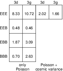
As for the cosmological analysis, we use scales between and arcmin. We also check the consistency of the E-mode signal with theory, in which case the assumed model is the WMAP9 prediction. Given the degrees of freedom 3 for the diagonal and 10 for the general third moment, the resulting is translated into a significance level. The results are shown in Fig. 5.
The significance of the E-mode is about when we include the cosmic variance. Using Poisson noise only, we obtain a much higher significance of more than . This covariance would be the correct one to use in case of absence of , since in this case there would be no cosmic variance. Thus, we can reject the hypothesis of a null third-order lensing signal with .
The signal is in very good agreement with the WMAP9 best-fit model. All diagonal B-mode components are less significant than the E-mode, and their amplitude is below the E-mode. However, both the generalised and generalised components are non-null at about .
4.4 Cosmological constraints
We test two predictions about third-order weak lensing statistics: (1) The generalised third-order aperture-mass moment contains more information about cosmology than the ‘diagonal’ term (Schneider et al. 2005; Kilbinger & Schneider 2005). (2) Combined with second-order, parameter degeneracies are partially lifted, leading to significantly improved joint constraints (Takada & Jain 2004; Kilbinger & Schneider 2005). We have already explored these two predictions using the CFHTLenS Clone simulations (Sect. A.1).
In Fig. 6, we show the marginalised constraints for and , the parameters that are best constraints from weak cosmological lensing. Symbols used in the following figures are explained in Table 3. The generalised third-order aperture-mass covers indeed a smaller part of parameter space compared to the diagonal one. Adding the non-equal smoothing scale measurements of the generalised third moment rules out those models with a very low and . The amplitude parameter is larger than zero at more than for both the diagonal and general third moment. This is at much higher significance than the non-zero detection of (previous section). This result is stronger, since it involves parameter fitting within the framework of an assuming theoretical model. In particular, the shape of the signal plays a role and adds information that is not used in a simple null test. This result is consistent with what we see in the Clone simulations.
| Symbol | Description |
|---|---|
| 2 | , aperture-mass dispersion |
| COSEBis, a second-order E-/B-mode measure (Schneider et al. 2010) | |
| 3d 44 4 Note that the symbol ‘3d’ indicates the third-moment diagonal, and is not to be confused with three-dimensional (3D) lensing, e.g. Kitching et al. (2014). | , diagonal third-order aperture-mass moment, evaluated for one filter scale |
| 3g | , generalised third-order aperture- mass moment, correlating three filter scales |
| SLC | (diagonal) third-order aperture-mass moment from source-lens clustering (Sect. 5.1) |
| IA | (diagonal) third-order aperture-mass moment from intrinsic alignments (Sect. 5.2) |
Diagonal and generalised third moment

Second, adding second-order measures reduces the allowed parameter space, however not by much as shown in Fig. 7. Third-order lensing probes a shallower slope of the parameter , in agreement with the theoretical prediction from Kilbinger & Schneider (2004) and Vafaei et al. (2010). Mainly in the region of extreme and is where the - and -constraints differ. The constraints orthogonal to the - degeneracy direction are reduced by % (%) when adding third-order to COSEBIs (aperture-mass dispersion). Here we see an example where a Fisher matrix analysis (Takada & Jain 2004; Kilbinger & Schneider 2005) can provide overly optimistic predictions (Wolz et al. 2012). Even though the slope of the constraints at the fiducial model is different, the curved, non-linear shape of the parameter degeneracy directions of the two probes largely negates this difference, leading to a larger overlap between the allowed regions. This shows the necessity to explore the full likelihood function, in our case with Monte-Carlo sampling, to obtain realistic joint constraints.
flat CDM

flat CDM

We explore extensions from the standard model CDM model, by adding (1) curvature, and (2) dark energy in the form of a constant equation-of-state parameter . For those extensions, the results on and are similar to the standard case, see Fig. 8. For further parameters, we combine CFHTLenS with other probes, see Sect. 6.
flat CDM

curved CDM

5 Astrophysical weak-lensing contaminants
Third-order cosmic shear statistics suffer from two major contaminants of astrophysical origin: Intrinsic alignment (IA) and source-lens clustering (SLC). Contrary to second-order statistics, IA and SLC contribute to a much higher level. The correlations they introduce can be comparable in amplitude to the cosmological weak-lensing skewness.
5.1 Source-lens clustering
Source-lens clustering (SLC), see Bernardeau (1998); Hamana et al. (2002), denotes the fact that galaxies in a weak-lensing survey act both as sources and lenses. More precisely, source galaxies are correlated to structures that cause the lensing effect on other source galaxies. For a given line of sight, this clustering gives rise to a modulation of the lensing signal, since the source redshift distribution is changed with respect to the average in a way that correlates with the lensing signal. This introduces an additional variance, skewness, etc. of the convergence field.
To model SLC, we have to use a locally-varying source galaxy density instead of the mean distribution , which are related to each other as
| (35) |
We assume a simple linear, deterministic galaxy bias and write
| (36) |
Inserting the modified galaxy distribution (35) into (3) leads to higher-order density correlations. These additional terms do not contribute more than a few percent to second-order statistics, since they are proportional to the convergence bispectrum. They are however of more importance for the third-order functions: both cosmic shear, for common models such as perturbation theory or HEPT, and SLC depend on terms that are proportional to the power spectrum squared. Inserting that additional convergence term into (10) yields the SLC contribution to the aperture-mass,
| (37) |
Note that we are not estimating the aperture-mass third moment from local measures of , for example by placing apertures over the survey and then computing the third moment of that distribution. Instead, we integrate over the 3PCF, which has been globally computed by averaging over all galaxy triples. Any local estimator would need to be normalised by the number of galaxies in that region, e.g. the aperture disk. That would include the SLC-corrected , partly off-setting the SLC contribution. In a perturbative ansatz, this is represented by two contributing terms with opposite signs (Bernardeau 1998). Our global estimators of the 3PCF (8, 9) are instead normalised by the number of galaxy triples over the whole survey. The SLC correction to that is very small compared to the expectation value of the unperturbed number of triples. Therefore, we can safely neglect this contribution (Valageas 2014).
We write the total aperture-mass as , and expand the third moment up to linear terms in the SLC contribution (37). The result is
| (38) |
The second term is the first-order SLC contribution. Inserting (37), this term can be written as
| (39) |
with
| (40) |
where is the modified Bessel function of order . This expression corresponds to the first term of equation (A17) in Hamana et al. (2002). The latter was obtained for a top-hat filter function, for which the two Fourier integrals separate. In our case of a compensated Gaussian filter, the closed expression (40) describes the mode coupling.
For the galaxy bias we take the redshift-scaling from Moscardini et al. (1998),
| (41) |
where is the linear growth factor. This implies a bias of unity at high redshift, which well matches our magnitude-limited sample (Giannantonio et al. 2014). At the bias is .
5.2 Intrinsic alignment
To model the contamination of galaxy intrinsic alignment (IA) to third-order cosmic shear, we implement the model from SHvWS08. This work measured IA in a suite of -body simulations, and modelled IA for different redshift ranges and a few simple galaxy populations.
For second-order cosmic shear with a very broad source redshift distribution as is the case in this work, intrinsic alignment plays a minor role. Its contamination of the cosmological lensing signal is of the order per cent (Benjamin et al. 2013), which we neglect here. See Heymans et al. (2013) for a measurement of second-order IA using narrow redshift bins. For third-order shear however, the contribution from IA is much larger, and we will model it as follows.
Third-order galaxy shape correlations including shear () and intrinsic shape () can be written schematically as a sum of the four terms . The first term, , is a pure lensing correlation. This is the quantity from which we deduce cosmological parameters. The last term, , is a pure intrinsic shape correlation. We can safely neglect this term, since only physically close galaxies give rise to this correlation. For our very wide redshift bin, the number of such close triples is very small compared to the overall number of galaxy triples. The expected amplitude is more than an order of magnitude smaller than GGG, an in fact consistent with zero for CFHTLS-type surveys (SHvWS08).
The mixed terms, stemming from the correlation between intrinsic shape and shear, are produced by galaxy triples at all redshift ranges, and can be very large compared to . The redshift scaling of these terms is easy to calculate, since it only depends on the geometry of the Universe. For the angular scaling, we follow SHvWS08 and assume a simple power-law dependence for the third-order aperture-mass.
Following Hirata & Seljak (2004), the redshift-dependence of the shear-shape (GI) correlation is straight-forwardly calculated. The lensing of a source galaxy at redshift by structures correlated to a galaxy at lens redshift scales as . For GGI and GII, we take into account the redshifts of the galaxy triple, and integrate over the redshift distributions, neglecting the clustering of galaxies as a higher-order contribution. Using a simple exponential scaling with angular distance (King 2005, SHvWS08) we obtain
| (42) |
The IA model parameters are the amplitudes and the characteristic angular scales and .
We add and to our theoretical third-order aperture-mass, and try to jointly sample cosmological and IA parameters. Due to the relatively low statistical significance of the CFHTLenS weak-lensing skewness and very limited redshift resolution, we do not aim to obtain interesting constraints on very general IA parameters. Rather, our goal is to use a realistic IA model to assess the influence on our cosmological results.
We therefore use the results from SHvWS08 as priors on our IA parameters. We use two models of the galaxy population: A realistic one (mixed early- and late-types) and a pessimistic case (early-types only). The redshift combinations tested in SHvWS08 closest to the CFHTLenS range correspond to the case of lens galaxies at and source galaxies at . This corresponds roughly to our mean source redshift of , and lens redshifts probed by a single redshift bin. The best-fit values and error bars for the four IA parameters are given in Table 4. We translate those into Gaussian priors with width equal to three times the error, while we exclude unphysical negative scales and .
5.3 Baryonic physics
The presence of baryons in dark-matter halos in the form of stars and gas changes halo properties compared to pure dark matter. This has an influence on the total power spectrum and bispectrum on small and medium scales. Prescriptions to quantify and model this, e.g. with a halo-model approach, have been obtained by using hydro-dynamical -body simulations (Jing et al. 2006; Rudd et al. 2008; van Daalen et al. 2011; Semboloni et al. 2011a, e.g.). The effect depends on the assumed details of baryonic physics. In the most realistic case, the amplitude of the third-order aperture moment at arcmin is suppressed by - per cent compared to dark matter only (Semboloni et al. 2013). Contrary to IA or SLC, the relative effect strongly decreases towards larger scales. At arcmin, the dark-matter only prediction is biased high by less than per cent.
We do not include a model of baryonic effects for the power- and bispectrum in this work. Using a simple calculation, where we model the decrease of as a function of angular scale according to Fig. 1 of Semboloni et al. (2013), we find that increases by () for the model with larger (smaller) baryonic suppression. So our value of , ignoring baryonic suppression, might be biased high by to per cent.
5.4 Results
flat CDM

| Model | arcmin | /arcmin | ||
|---|---|---|---|---|
| mixed (realistic) | ||||
| elliptical (pessimistic) |
curved CDM

Adding IA and SLC changes the amplitude parameter within the statistical uncertainty of CFHTLenS. The amplitude change is comparible in size with the difference between the diagonal and generalized third moments, see Fig. 9.
As expected, the total IA contribution ( plus ) reduces the skewness, and the amplitude parameter increases to compensate. There is only a mild degeneracy between and the IA amplitudes and . The same is true for the . The two IA amplitude parameters are strongly anti-correlated, since they contribute to the skewness with opposite sign. The posterior error bars on the IA amplitude decrease by about 20% with respect to the prior.
Using the purely elliptical model from SHvWS08 leads to a very strong decrease of the third moments. This is the case within the full prior range, which we take to be three times as large as the errors of SHvWS08. The resulting cosmic shear plus IA aperture-mass skewness is not compatible with our measurement, and we conclude that this model is not supported by the data.
SLC leads to a increase of the skewness contrary to IA, and therefore the jointly fitted is smaller compared to ignoring this astrophysical systematic. We explored different bias models and marginalise over a range of parameters. We found that the results are not very sensitive within a reasonable model space. The results presented in this paper correspond to a flat prior with . The magnitude-limited sample of lensing-selected galaxies between redshifts of 0.2 and 1.3 is expected to have a mean bias that is not too far from unity.
When both IA and SLC are included in the joint second- plus third-order lensing analysis, the resulting amplitude parameter is marginally increased (Table 5).
flat CDM
curved CDM

 ,
,
6 Joint parameter constraints
| Parameter | flat CDM | flat CDM | curved CDM |
|---|---|---|---|
We add CMB to CFHTLenS weak-lensing, to lift some of the parameter constraints. Throughout this section, the weak-lensing data consists of the second-order COSEBIs combined with third-order diagonal aperture mass. For the latter we include intrinsic alignment and source-lens clustering (Sect. 5). We do not include a model of the baryonic modification of the power- and bispectrum. With the conservative choice of angular scales, we limit the influence of small-scale model unertainties, see also Sect. 5.3.
It is well-known (Contaldi et al. 2003) and has been recently been demonstrated again in K13, that the - lensing degeneracy in a flat CDM model can be lifted by the addition of CMB anisotropies, since the latter shows a near-orthogonal correlation between those two parameters. In this paper, we combine second- and third-order CHFLTenS weak lensing with WMAP9 and Planck measurements. The results are shown in Table 6.
The Planck constraints are much tighter than the ones from WMAP, and do therefore dominate the combined confidence region. The Planck error region is around a slightly higher but there is no significant tension.
For a non-flat cosmology, the difference between WMAP9 and Planck is much more pronounced, since Planck alone measures the curvature of the Universe to a high precision due to the addition of CMB lensing (Smith et al. 2006). Moreover, the small size of the joint constraints for CHFLTenS + Planck comes partially from the fact that the two confidence regions have a smaller overlap. We do not consider this to be a tension: both probes are consistent at 95% confidence.
The density of the cosmological constant, is not well constrained by 2D lensing. However, the strong degeneracy for CMB alone, which is close to the direction of constant curvature, can be lifted when adding both probes (Fig. 10). This is also true for Planck, where the degeneracy is smaller due its sensitivity to CMB lensing, but the joint CHTLenS+Planck constraints are smaller by . Note that the joint CFHTLenS+Planck contour is shifted to lower values of compared to Planck alone, due to the differences for between the two probes, see Fig. 11. For a given , CFHTlenS prefers a lower .
The CFHTLenS+Planck constraints are shifted towards smaller compared to Planck alone (Figs. 10 and 11). It was already seen from second-order cosmic shear (Benjamin et al. 2013; Heymans et al. 2013, K13;) that CFHTLenS prefers a lower . Further, over the range of allowed by Planck, lensing puts a lower limit on . Because of the strong CMB degeneracies between and both and , the joint Lensing+Planck constraints rule out larger values of and (Fig. 12).
For a flat CDM model with a free, constant parameter, the CMB shows the same degeneracy as weak lensing in the space of and as shown in Kilbinger et al. (2009). Adding WMAP9 to CFHTLenS does not reduce the allowed parameter space by much – to lift the degeneracy efficiently, one would have to further add BAO and/or Hubble constant priors. The combined CFHTLenS+Planck contours are dominated by Planck. Compared to the flat case, the allowed parameter space moves towards lower and higher .
curved CDM

curved CDM

| Param. | flat CDM | flat CDM | curved CDM |
|---|---|---|---|

7 Discussion
7.1 Diagonal and generalized third moments
The generalised third-order aperture-mass contains more information about cosmology than the diagonal one (Kilbinger & Schneider 2005). This is because the former probes a wide range of triangles of different shape of the bispectrum in Fourier space. The latter is restricted to mainly equilateral triangles. This can be inferred from eq. (13): if all filter scales are equal, the filter functions all peak at the same scale , and the bispectrum contribution comes mainly from equilateral triangles.
We confirm this prediction with CFHTLenS, where the error bar on the amplitude parameter is reduced to about half the size (Fig. 13, Table 7). Most importantly, the generalized third moment excludes a good part of the low-amplitude region in the - parameter space (Fig. 6). Interestingly, despite this information increase, the detection significance of the generalised third moment is lower than for the diagonal case (Fig. 5). That shows that the null test is sensitive to different properties of the measurement than the Bayesian parameter fit. In particular, there is extra-information in the shape of the signal, and not only in the amplitude. Only the latter plays a role for the null test.
This increase in information for the generalised third moment is also seen in the Clone simulation, albeit less pronounced. Despite our attempt to create simulations as realistic as possible, there are differences which might influence the third-moment measurement in the Clone in a different way compared to the data. This could be the noise, but also the underlying cosmological skewness which might be affected by the finite field and discretisation in the Clone.
The mean value of is larger for the generalised third moment compared to the diagonal case. The difference is not significant due to the relative large error, but we see the same trend with the Clone simulation. This may be because the bispectrum model is not well calibrated on non-equilateral triangles. Another reason could be that the numerical integration over the 3PCF performs more poorly for non-equal aperture radii, and gives biased results. This possibility has to be explored in the future with larger simulations.
7.2 E- and B-modes
We obtained a measurement of the cosmic shear third-order correlations from CFHTLenS data, but also three cases of B-mode combinations that are inconsistent with zero at . One of these detections, the generalised , signifies a violation of parity invariance. It is not very likely that an astrophysical source is at the origin of this mode, since it would require a model with a preferred orientation.
We tested the algorithm to calculate the third-order aperture on the Clone simulations, and did not find a significant B-mode. It is however possible that numerical issues are at the root of the B-mode, such as the discreteness of the triangle binning of the 3PCF, or of the numerical integration of the 3PCF to obtain the aperture quantities, or incomplete available integration range. The fact that the significance of two of the B-mode components ( and ) is larger for the generalised third moment is compatible with this view, since the integration kernels are different for the case with three different filter scales. More work is however required to scrutinise this hypothesis.
Undetected PSF correction residuals could be responsible for this B-mode. Third-order PSF-shear correlations were tested and the 120 fields used in this work were statistically found to be free of systematics (Semboloni et al. 2014), based on error estimates using CFHTLenS Clone simulations, which includes Poisson noise and cosmic variance. As in Heymans et al. (2012), these tests were done in a cosmology-blind way, and therefore did not include E- and B-mode decompositions. A full analysis of E- and B-modes from PSF residuals is left for future work.
Further, the lack of intrinsic alignment in the Clone simulations might lead to an under-estimation of the covariance matrix, if IA produces B-modes, which is very plausible: Capranico et al. (2013) obtain E- and B-mode IA power spectrum from a generic angular momentum model. SHvWS08 calculate the B-mode term using simple halo-galaxy ellipticity correlations in N-body simulations, and find a similar amplitude compared to the E-mode. IA generates cosmic variance for the B-mode components, which our covariance estimate does not include. This might lead to an over-estimation of the B-mode significance. To test this hypthesis requires a realistic IA model that produces B-modes.
7.3 Astrophysical systematics
We included simple models of two major astrophysical contaminations to the third-order shear observables. Both intrinsic alignment and source-lens clustering depend on the relation of galaxies and dark matter, and are therefore notoriously difficult to model.
Both IA and SLC modulate the lensing third-order statistics, but the change on is smaller than the 68% statistical error in both cases. The error bars on this parameter do not increase when adding those systematic contributions.
IA consists of two relevant components ( and ) with opposite sign. Even though the amplitude of each component can be large, their sum cancels out to a large part. The total contribution to the third moment is negative. Our adopted galaxy model consists of a mixture of early- and late-type galaxies. A pure elliptical sample would produce a very large IA skewness, which is ruled out by our cosmic shear data.
The SLC contribution is proportional to the galaxy bias. We found that the resulting constraints are not very sensitive to the bias model. However, for future precision measurements the bias of the lensing galaxy sample has to be known very well. This is true in particular for tomographic weak lensing, where galaxies at different redshifts create an SLC signal that depends on the bias as a function of redshift.
We do not include the effect of baryons on the power- and bispectrum. With the conservative choice of angular scales, we limit the influence of small-scale model unertainties. Following the results from -body simulations from Semboloni et al. (2013), we estimate that the lensing amplitude parameter from third-order alone might be biased high between and per cent.
7.4 Binning of the three-point correlation function
We obtain the third-order aperture-mass moment from the shape catalogue by integrating over the measured and binned three-point shear correlation function (3PCF). The computation time, even using a fast tree code, limits us in the use of very small bins. We explore a range of bin sizes using the Clone simulations, and find convergence of the results for a reasonable computation time. However, we do see larger differences in the resulting amplitude of from the data as a function of bin size (App. A.2). The differences are well within the statistical uncertainty of the data, and we leave a more detailed exploration of the 3PCF calculation for future work.
7.5 Limitations of cosmology from third-order shear statistic
Currently, there are limitation for the use of weak-lensing skewness measures for precision cosmology. These include:
- •
Model predictions of the bispectrum. Current fitting formulae of the bispectrum are accurate to only 10% on small scales (Gil-Marín et al. 2012). Moreover, these models have been calibrated to only a few basic cosmological models such as CDM. More accurate models are needed, spanning a larger parameter space including dark-energy cosmologies. We tested several models in App. A.1.
Further, the effect of baryons has to be studied and quantified, for which it is necessary to run large hydro-dynamical -body simulations. Predictions based on the halo model have already been made for third-order statistics (Semboloni et al. 2013). On small scales our lack of knowledge of baryonic physics become the dominant uncertainty for weak lensing cosmological results.
- •
Astrophysical systematics are not well understood. In particular intrinsic alignment models are too simplistic for future large-area surveys. Alternatively, IA can be largely removed via nulling, at the price of significant loss of constraining power (Shi et al. 2010). SLC is easier to model, since it only involves the bias of the lensing galaxy sample, which can be obtained with independent observations, for example using galaxy clustering.
- •
The Gaussian approximation of the likelihood function will not be sufficient for future surveys. Numerical simulations can be used to explore and estimate the true likelihood function for a limited parameter set (Hartlap et al. 2009; Pires et al. 2009). In App. A.3 we calculate the distribution of the third-order aperture-mass measurements.
In this work we tested and used simple approaches to mitigate those limitations in the view of current state-of-the-art weak lensing data. Different models of the bispectrum were compared, intrinsic alignment was modelled and jointly constrained with cosmology, and the Gaussianity of the data was measured, and, in the companion paper Semboloni et al. (2014), a non-Gaussian likelihood model was employed.
Acknowledgments
The authors thank M. Jarvis for kindly providing his code to compute the three-point correlation functions. We acknowledge A. Grado for providing the VST cluster at Naples Observatory for computation time, and P. Schneider and P. Valageas for fruitful discussions. We thank the anonymous referee for useful comments.
This work is based on observations obtained with MegaPrime/MegaCam, a joint project of CFHT and CEADAPNIA, at the Canada-France-Hawaii Telescope (CFHT) which is operated by the National Research Council (NRC) of Canada, the Institut National des Sciences de l’Univers of the Centre National de la Recherche Scientifique (CNRS) of France, and the University of Hawaii. This research used the facilities of the Canadian Astronomy Data Centre operated by the National Research Council of Canada with the support of the Canadian Space Agency. We thank the CFHT staff for successfully conducting the CFHTLS observations and in particular Jean-Charles Cuillandre and Eugene Magnier for the continuous improvement of the instrument calibration and the Elixir detrended data that we used. We also thank TERAPIX for the individual exposures quality assessment and validation during the CFHTLS data acquisition period, and Emmanuel Bertin for developing some of the software used in this study. CFHTLenS data processing was made possible thanks to significant computing support from the NSERC Research Tools and Instruments grant program, and to HPC specialist Ovidiu Toader.
LF acknowledges support from NSFC grants 11103012 &11333001, Innovation Program 12ZZ134 of SMEC, STCSM grant 11290706600, and Shanghai Research grant 13JC1404400. MJH acknowledges support from the Natural Sciences and Engineering Research Council of Canada (NSERC). MK is supported in parts by the DFG cluster of excellence ‘Origin and Structure of the Universe’. CH acknowledges support from the European Research Council under the EC FP7 grant number 240185. TDK acknowledges support from a Royal Society University Research Fellowship. LVW acknowledges support from the Natural Sciences and Engineering Research Council of Canada (NSERC) and the Canadian Institute for Advanced Research (CIfAR, Cosmology and Gravity program). TE is supported by the Deutsche Forschungsgemeinschaft through project ER 327/3-1 and the Transregional Collaborative Research Centre TR 33 - ”The Dark Universe”. H. Hildebrandt is supported by the Marie Curie IOF 252760, by a CITA National Fellowship, and the DFG grant Hi 1495/2-1. H. Hoekstra acknowledges support from Marie Curie IRG grant 230924, the Netherlands Organisation for Scientific Research (NWO) grant number 639.042.814 and from the European Research Council under the EC FP7 grant number 279396. YM acknowledges support from CNRS/INSU (Institut National des Sciences de l’Univers) and the Programme National Galaxies et Cosmologie (PNCG). BR acknowledges support from the European Research Council in the form of a Starting Grant with number 240672. MJH acknowledges support from the Natural Sciences and Engineering Research Council of Canada (NSERC). TS acknowledges support from NSF through grant AST-0444059-001, SAO through grant GO0-11147A, and NWO. MV acknowledges support from the Netherlands Organization for Scientific Research (NWO) and from the Beecroft Institute for Particle Astrophysics and Cosmology. The -body simulations used in this analysis were performed on the TCS supercomputer at the SciNet HPC Consortium. SciNet is funded by: the Canada Foundation for Innovation under the auspices of Compute Canada; the Government of Ontario; Ontario Research Fund - Research Excellence; and the University of Toronto.
Author Contribution: All authors contributed to the development and writing of this paper. The authorship list consists of three alphabetic groups: The first group indicates the two lead authors of this paper (LF, MK). The second group includes key contributers to the science analysis and interpretation in this paper, the founding core team and those whose long-term significant effort produced the final CFHTLenS data product. The third group covers members of the CFHTLenS team who made a significant contribution to the project and/or the paper. The CFHTLenS collaboration was co-led by CH and LVW, and the CFHTLenS Cosmology Working Group was led by TK.
References
- Anderson (2003) Anderson T. W., 2003, An introduction to multivariate statistical analysis, 3rd edn. Wiley-Interscience
- Bartelmann (2010) Bartelmann M., 2010, Classical and Quantum Gravity, 27, 233001
- Bartelmann & Schneider (2001) Bartelmann M., Schneider P., 2001, Phys. Rep., 340, 297
- Benjamin et al. (2013) Benjamin J. et al., 2013, \mnras, 431, 1547
- Bernardeau (1998) Bernardeau F., 1998, \aap, 338, 375
- Bernardeau et al. (1997) Bernardeau F., Van Waerbeke L., Mellier Y., 1997, \aap, 322, 1
- Bernardeau et al. (2003) Bernardeau F., Van Waerbeke L., Mellier Y., 2003, \aap, 397, 405
- Capranico et al. (2013) Capranico F., Merkel P. M., Schäfer B. M., 2013, \mnras, 435, 194
- Contaldi et al. (2003) Contaldi C. R., Hoekstra H., Lewis A., 2003, Physical Review Letters, 90, 221303/1
- Crittenden et al. (2002) Crittenden R. G., Natarajan P., Pen U.-L., Theuns T., 2002, \apj, 568, 20
- Eifler et al. (2009) Eifler T., Schneider P., Hartlap J., 2009, \aap, 502, 721
- Erben et al. (2013) Erben T. et al., 2013, \mnras, 433, 2545
- Fu et al. (2008) Fu L. et al., 2008, \aap, 479, 9
- Giannantonio et al. (2014) Giannantonio T., Ross A. J., Percival W. J., Crittenden R., Bacher D., Kilbinger M., Nichol R., Weller J., 2014, \prd, 89, 023511
- Gil-Marín et al. (2012) Gil-Marín H., Wagner C., Fragkoudi F., Jimenez R., Verde L., 2012, \jcap, 2, 47
- Hamana et al. (2002) Hamana T., Colombi S. T., Thion A., Devriendt J. E. G. T., Mellier Y., Bernardeau F., 2002, \mnras, 330, 365
- Harnois-Déraps et al. (2012) Harnois-Déraps J., Vafaei S., Van Waerbeke L., 2012, \mnras, 426, 1262
- Hartlap et al. (2009) Hartlap J., Schrabback T., Simon P., Schneider P., 2009, \aap, 504, 689
- Hartlap et al. (2007) Hartlap J., Simon P., Schneider P., 2007, \aap, 464, 399
- Heitmann et al. (2009) Heitmann K., Higdon D., White M., Habib S., Williams B. J., Lawrence E., Wagner C., 2009, \apj, 705, 156
- Heitmann et al. (2014) Heitmann K., Lawrence E., Kwan J., Habib S., Higdon D., 2014, \apj, 780, 111
- Heitmann et al. (2010) Heitmann K., White M., Wagner C., Habib S., Higdon D., 2010, \apj, 715, 104
- Heymans et al. (2013) Heymans C. et al., 2013, \mnras, 432, 2433
- Heymans et al. (2012) Heymans C. et al., 2012, \mnras, 427, 146
- Hildebrandt et al. (2012) Hildebrandt H. et al., 2012, \mnras, 421, 2355
- Hirata & Seljak (2004) Hirata C. M., Seljak U., 2004, \prd, 70, 063526
- Hoekstra & Jain (2008) Hoekstra H., Jain B., 2008, Annual Review of Nuclear and Particle Science, 58, 99
- Jarvis et al. (2004) Jarvis M., Bernstein G., Jain B., 2004, \mnras, 352, 338 (JBJ04)
- Jee et al. (2013) Jee M. J., Tyson J. A., Schneider M. D., Wittman D., Schmidt S., Hilbert S., 2013, \apj, 765, 74
- Jing et al. (2006) Jing Y. P., Zhang P., Lin W. P., Gao L., Springel V., 2006, \apjl, 640, L119
- Kaiser (1992) Kaiser N., 1992, \apj, 388, 272
- Kaiser et al. (1994) Kaiser N., Squires G., Fahlman G., Woods D., 1994, in Clusters of galaxies, Proceedings of the XIVth Moriond Astrophysics Meeting, Méribel, France, p. 269, alsoarXiv:astro-ph/9407004
- Kayo et al. (2013) Kayo I., Takada M., Jain B., 2013, \mnras, 429, 344
- Kilbinger et al. (2009) Kilbinger M. et al., 2009, \aap, 497, 677
- Kilbinger et al. (2013) Kilbinger M. et al., 2013, \mnras, 430, 2200 (K13)
- Kilbinger & Schneider (2004) Kilbinger M., Schneider P., 2004, \aap, 413, 465
- Kilbinger & Schneider (2005) Kilbinger M., Schneider P., 2005, \aap, 442, 69
- Kilbinger et al. (2006) Kilbinger M., Schneider P., Eifler T., 2006, \aap, 457, 15
- King (2005) King L. J., 2005, \aap, 441, 47
- Kitching et al. (2014) Kitching T. D. et al., 2014, submitted to \mnras, also 1401.6842
- Lawrence et al. (2010) Lawrence E., Heitmann K., White M., Higdon D., Wagner C., Habib S., Williams B., 2010, \apj, 713, 1322
- Miller et al. (2013) Miller L. et al., 2013, \mnras, 429, 2858
- Moscardini et al. (1998) Moscardini L., Coles P., Lucchin F., Matarrese S., 1998, \mnras, 299, 95
- Munshi et al. (2008) Munshi D., Valageas P., Van Waerbeke L., Heavens A., 2008, \physrep, 462, 67
- Peacock & Dodds (1996) Peacock J. A., Dodds S. J., 1996, \mnras, 280, L19
- Peebles (1980) Peebles P. J. E., 1980, The Large-Scale Structure of the Universe. Princeton University Press
- Pen et al. (2003) Pen U.-L., Zhang T., Van Waerbeke L., Mellier Y., Zhang P., Dubinski J., 2003, \apj, 592, 664
- Pires et al. (2009) Pires S., Starck J.-L., Amara A., Réfrégier A., Teyssier R., 2009, \aap, 505, 969
- Planck Collaboration et al. (2014) Planck Collaboration et al., 2014, \aap in press, also 1303.5076
- Rudd et al. (2008) Rudd D. H., Zentner A. R., Kravtsov A. V., 2008, \apj, 672, 19
- Sato & Nishimichi (2013) Sato M., Nishimichi T., 2013, \prd, 87, 123538
- Schneider (1996) Schneider P., 1996, \mnras, 283, 837
- Schneider (2003) Schneider P., 2003, \aap, 408, 829
- Schneider et al. (2010) Schneider P., Eifler T., Krause E., 2010, \aap, 520, A116
- Schneider et al. (2005) Schneider P., Kilbinger M., Lombardi M., 2005, \aap, 431, 9 (SKL05)
- Schneider & Lombardi (2003) Schneider P., Lombardi M., 2003, \aap, 397, 809
- Schneider et al. (1998) Schneider P., Van Waerbeke L., Jain B., Kruse G., 1998, \mnras, 296, 873
- Schneider et al. (2002) Schneider P., Van Waerbeke L., Mellier Y., 2002, \aap, 389, 729
- Schrabback et al. (2010) Schrabback T. et al., 2010, \aap, 516, A63
- Scoccimarro & Couchman (2001) Scoccimarro R., Couchman H. M. P., 2001, \mnras, 325, 1312
- Semboloni et al. (2008) Semboloni E., Heymans C., van Waerbeke L., Schneider P., 2008, \mnras, 388, 991 (SHvWS08)
- Semboloni et al. (2013) Semboloni E., Hoekstra H., Schaye J., 2013, \mnras, 434, 148
- Semboloni et al. (2011a) Semboloni E., Hoekstra H., Schaye J., van Daalen M. P., McCarthy I. G., 2011a, \mnras, 417, 2020
- Semboloni et al. (2011b) Semboloni E., Schrabback T., van Waerbeke L., Vafaei S., Hartlap J., Hilbert S., 2011b, \mnras, 410, 143
- Semboloni et al. (2014) Semboloni E., et al., 2014, in prep.
- Shi et al. (2010) Shi X., Joachimi B., Schneider P., 2010, \aap, 523, A60
- Shi et al. (2014) Shi X., Joachimi B., Schneider P., 2014, \aap, 561, A68
- Smith et al. (2006) Smith K. M., Hu W., Kaplinghat M., 2006, \prd, 74, 123002
- Smith et al. (2003) Smith R. E. et al., 2003, \mnras, 341, 1311
- Takada & Jain (2003) Takada M., Jain B., 2003, \apjl, 583, L49
- Takada & Jain (2004) Takada M., Jain B., 2004, \mnras, 348, 897
- Takahashi et al. (2012) Takahashi R., Sato M., Nishimichi T., Taruya A., Oguri M., 2012, \apj, 761, 152
- Taylor et al. (2013) Taylor A., Joachimi B., Kitching T., 2013, \mnras
- Vafaei et al. (2010) Vafaei S., Lu T., van Waerbeke L., Semboloni E., Heymans C., Pen U.-L., 2010, Astroparticle Physics, 32, 340
- Valageas (2014) Valageas P., 2014, \aap, 561, A53
- van Daalen et al. (2011) van Daalen M. P., Schaye J., Booth C. M., Dalla Vecchia C., 2011, \mnras, 415, 3649
- Van Waerbeke et al. (2013) Van Waerbeke L. et al., 2013, \mnras, 433, 3373
- Van Waerbeke et al. (1999) Van Waerbeke L., Bernardeau F., Mellier Y., 1999, \aap, 342, 15
- Van Waerbeke et al. (2001) Van Waerbeke L., Hamana T., Scoccimarro R., Colombi S., Bernardeau F., 2001, \mnras, 322, 918
- Wolz et al. (2012) Wolz L., Kilbinger M., Weller J., Giannantonio T., 2012, \jcap, 9, 9
- Zaldarriaga & Scoccimarro (2003) Zaldarriaga M., Scoccimarro R., 2003, \apj, 584, 559
Appendix A Clone simulation tests
In this appendix we discuss various tests involving the CFHTLenS ‘Clone’ -body simulations (Harnois-Déraps et al. 2012). These tests include the validity of the theoretical model, and the accuracy of the 3PCF algorithm.
A.1 Theoretical model and angular scales
To check the accuracy of our theoretical model as well as the numerical algorithms involved to obtain the third-order aperture-mass moments, we measure from the Clone simulation and try to recover the input cosmology using the sampling method and likelihood function as described in the previous two sections. We implemented various combinations of prescriptions of the non-linear power and bi-spectrum as described at the end of Sect.2.1. A comparison of those predictions with the Clone simulations are shown in Fig. 14. The difference between the original halofit (Smith et al. 2003) and its revised version is minimal for third order. The difference with Heitmann et al. (2014) is larger but still small compared to our error bars. Since the validity of the latter is restricted in parameter space, -, and redshift range, we chose the revised halofit prescription for the power spectrum. The model from Gil-Marín et al. (2012) overpredicts the Clone simulations, and we choose Scoccimarro & Couchman (2001) for the bispectrum model.

We try different combinations of minimum and maximum aperture radii under the assumption of a flat CDM model. The parameter combination , which is the direction along the degeneracy, is consistent with the input value of . The best recovery of the input parameters is obtained using the aperture angular range [. We therefore choose this range for the cosmological analysis of CFHTLenS, using three filter scales. The number of distinct data points for the generalised third moment (combinations with repetitions) is 10.
The generalised third moment yields only sightly smaller error bars compared to the diagonal case, thereby only partially confirming the predicted strong increase of information from Fisher matrix analyses (Kilbinger & Schneider 2005). In Sect. 4.4 we see that the CFHTLenS data shows a larger difference between diagonal and generalised third moment. This is further elaborated in the discussion (Sect. 7).
We compare third-order constraints with the aperture-mass dispersion , the latter ranging between 2 to 70 arcmin. The direction of degeneracy for and is very similar in both cases, but the slope of the elongated “banana” is slightly steeper for the dispersion than for the third moment, in agreement with theoretical predictions (Kilbinger & Schneider 2005; Vafaei et al. 2010).
Our smallest angular scale for second- (third-) order is . This corresponds to a Fourier scale of about . Since the filter functions decay exponentially, we are not sensitive to . At the redshift of peak lensing efficiency (, this corresponds to 3D Fourier scales of of . At redshift of , below which the large-scale structure contributes less than 10% to the overall lensing signal, the corresponding -mode is /Mpc.
A.2 Calculating the 3PCF and binning of triangles
We obtain the third-order aperture-mass moment from the shape catalogue by integrating over the measured and binned three-point shear correlation function (3PCF). The computation time, even using a fast tree code, limits us in the use of very small bins. The tree-code from JBJ04 uses equidistant bins of size in the logarithm of the triangle side lengths. We explore various bin sizes using a subsample of 20 out of 184 simulated Clone fields. As shown in the top panel of Fig 15, large bin sizes underestimate the signal. However, we find convergence of the results for bin sizes smaller than . Based on these findings, we choose the conservative bin size for the CFHTLenS data.
When applying bin sizes and to CFHTLenS data, we do see slightly larger differences in the resulting amplitude of (see the bottom panel of Fig 15). The differences are well within the statistical uncertainty of the data, and we leave a more detailed exploration of the 3PCF calculation for future work.
Clone

CFHTLenS

A.3 Distribution of the third moment measurements
We use a Gaussian likelihood function (34) of our data as an approximation of the true likelihood function. Semboloni et al. (2014) consider a non-Gaussian treatment of the likelihood function using an independent component analysis (ICA) with the help of numerical simulations. They found that the effect on cosmological parameters is minor. Thus, the Gaussian likelihood functions still represents a good approximation.
To further test this assumption, we compute the distribution of the aperture-mass skewness from realisations of the Clone including intrinsic galaxy ellipticity noise. The results are printed in Table 8. The rms of the skewness and kurtosis from a Gaussian distribution with unknown mean are and , respectively. There is a marginal detection of a negative kurtosis at large scales. The skewness is consistent with zero. We conclude that the assumption of a Gaussian distribution for is sufficient for our purpose.
| Scale | ||||||
|---|---|---|---|---|---|---|
| Skewness | ||||||
| Kurtosis | ||||||