跳到论文正文
W Papers独立论文阅读器 arXiv:1404.5465 论文正文 计算阅读时间 · 0%
引用这篇论文根据当前论文元数据生成,正式投稿前建议核对。


License: arXiv.org perpetual non-exclusive license
arXiv:1404.5465v2 [math.ST] 24 Oct 2016

Best prediction under a nested error model with log transformation

Supported by the Spanish grants SEJ2007-64500, MTM2012-37077-C02-01, MTM-2012-33740 and ECO-2011-25706. Part of this work was done during a research stay of the second author in the Institute of Statistics of the University of Neuchâtel.
Nirian Martín    Isabel Molina Affiliation: Department of Statistics, Universidad Carlos III de Madrid

Key words: Empirical best estimator; Mean squared error; Parametric bootstrap.
MSC 2000: primary 62D05; secondary 62G09.


Abstract: In regression models involving economic variables such as income, log transformation is typically taken to achieve approximate normality and stabilize the variance. However, often the interest is predicting individual values or means of the variable in the original scale. Back transformation of predicted values introduces a non-negligible bias. Moreover, assessing the uncertainty of the actual predictor is not straightforward. In this paper, a nested error model for the log transformation of the target variable is considered. Nested error models are widely used for estimation of means in subpopulations with small sample sizes (small areas), by linking all the areas through common parameters. These common parameters are estimated using the overall set of sample data, which leads to much more efficient small area estimators. Analytical expressions for the best predictors of individual values of the original variable and of small area means are obtained under the nested error model with log transformation of the target variable. Empirical best predictors are defined by estimating the unknown model parameters in the best predictors. Exact mean squared errors of the best predictors and second order approximations to the mean squared errors of the empirical best predictors are derived. Mean squared error estimators that are second order correct are also obtained. An example with Mexican data on living conditions illustrates the procedures.

1 Introduction

In Econometric regression models, variables such as income or expenditure are often transformed with logarithm to achieve homoscedastic errors with approximately normal distribution. However, the variable of interest remains to be the untransformed one. Target characteristics of the study variable such as the values for out-of-sample individuals or the means for specific subpopulations become then functions of the exponentials of the dependent variable in the model. However, the predictors obtained by transforming back the individual predicted values are biased. Usual bias-corrections are only approximations and optimality properties are lost. However, the exact expression for the optimal predictors can be obtained analytically for certain models. A model that is often used for small area estimation is the nested-error linear regression model proposed by Battesse, Harter and Fuller (1988) to estimate the area under production of corn and soybeans in a number of counties. In small area estimation, the lack of sample observations in some of the areas of interest is solved by linking all areas through the common regression parameters but including at the same time random area effects that represent the unexplained between area variation. The common parameters are estimated using the sample observations from all the areas together and this leads to great efficiency gains with respect to estimators that use only the area-specific sample data (direct estimators). This kind of model is used in Econometric applications as well, see e.g. Elbers, Lanjouw and Lanjouw (2003) or Molina and Rao (2010), who employed this model to estimate poverty indicators in small areas. For more details on small area estimation methods, see the monograph by Rao and Molina (2015) and the recent review by Pfeffermann (2013).

Assessing the reliability, or uncertainty, of the obtained predictors is crucial in practical applications. A popular uncertainty measure is the mean squared error (MSE), also called mean squared prediction error. MSEs of optimal predictors of small area parameters have been obtained under certain models but only for simple parameters, see e.g. Das, Jiang and Rao (2004). The MSE of an individual prediction under a nested-error model with log-transformation that is second-order correct has not been obtained yet. Moreover, when predicting the mean of the original variable in a given area, the optimal predictor is function of the predicted values for the out-of-sample individuals from that area. Since the individuals belong to the same area, due to the presence of the area effects, individual predictors are not independent. Then mean crossed product errors (MCPEs) between pairs of individual predictions are needed to derive the MSE of the predictor of the mean in that area.

Here we obtain optimal predictors for individual values of the target variable in out-of-sample units and also for small area means. Additionally, second-order asymptotic approximations for the MCPEs of pairs of individual predictions are derived, which lead to good approximations for the MSEs of predicted area means. In the small area estimation literature, this was done previously only under area-level models by Slud and Maiti (2006). Under a unit-level model, Molina (2009) dealt with estimation of exponentials of mixed effects, i.e. exponentials of linear functions of the fixed and the random effects in the model; the individual values of the original variable cannot be expressed as special cases of these parameters. Thus, the target parameters and not the same and consequently results are also different. In particular, certain crossed-product terms appearing in the MCPE that are of lower order in Molina (2009), are not negligible when predicting individual observations. In fact, those crossed-product terms are typically neglected in small area estimation applications. Here we show that these terms cannot be neglected and give their analytical expression up to o⁡(D−1)o(D^{-1}) terms, where DD is the number of areas.

Analytical approximations for the uncertainty measures have a complex shape and users might prefer to use resampling procedures such as bootstrap methods. González-Manteiga et al. (2008) proposed a parametric bootstrap method designed for finite populations under a nested error model that is suitable in this paper. However, González-Manteiga et al. (2008) proved consistency of the bootstrap MSE estimator when the target parameters are linear. For our particular non-linear parameters, consistency remains to be proved. Nevertheless, once an analytical asymptotic expression is available for the true MSE, the technique of imitation used in that paper can be followed to achieve the consistency in this paper. Thus, the theoretical results for the MSE approximation that are obtained in this paper lead automatically to the consistency of the corresponding bootstrap MSE estimators.

The paper is organized as follows. The considered model and the target quantities are introduced in Section 2. This section also gives the best predictor and first and second-stage empirical best predictors of the target quantities. Section 3 describes usual likelihood-based fitting methods. MCPEs and MSEs of first-stage empirical best predictors are obtained in Section 4, and for second-stage empirical best predictors, second-order approximations to the analogous uncertainty measures are given in Section 5. Second-order unbiased estimators of these uncertainty measures are provided in Section 6. Section 7 describes a parametric bootstrap procedure for estimation of the uncertainty. Section 8 describes the result of a simulation experiment comparing the proposed predictor with existing ones. Section 9 illustrates the procedures through the estimation of mean income in municipalities from Mexico. Finally, the proofs of all the theorems are included in the Appendix.

2 Model, target quantities and predictors

When estimating characteristics of subpopulations that have varying sizes, it seems convenient to work under a finite population setup. Here we consider that the population UU is finite and contains NN units. This population is partitioned into DD subpopulations U1,…,UDU_{1},\ldots,U_{D}, also called areas or domains, of sizes N1,…,NDN_{1},\ldots,N_{D}. The data is obtained from a sample ss of size nn drawn from the population UU. We denote by sds_{d} the subsample from domain dd, of (fixed) size ndn_{d}, d=1,…,Dd=1,\ldots,D, with ∑d=1Dnd=n\sum_{d=1}^{D}n_{d}=n, and by s¯d=Ud−sd\bar{s}_{d}=U_{d}-s_{d} the sample complement from area dd, of size Nd−ndN_{d}-n_{d}, d=1,…,Dd=1,\ldots,D.

The goal is to predict the value wd​iw_{di} of the variable of interest for an out-of-sample individual ii within area dd, or the area mean Nd−1​∑i=1Ndwd​iN_{d}^{-1}\sum_{i=1}^{N_{d}}w_{di}, based on a regression model for wd​iw_{di}. If wd​iw_{di} represents a measurement of an economical variable such as income or expenditure, it is customary to consider the logarithm of wd​iw_{di} as dependent variable in a regression model. Moreover, in many applications, the available auxiliary variables do not explain sufficiently well all the between-area variation that data exhibit. Then, random area effects representing this unexplained variation are included in the model. This is typically done in small area estimation applications. Here we assume the following linear regression model with random area effects, also known as nested-error model, for the log-transformed variables yd​i=log⁡wd​iy_{di}=\log w_{di},

yd​i=𝐱d​i′​𝜷+ud+ed​i,ud​∼i​i​d​𝒩​(0,σu2),ed​i​∼i​i​d​𝒩​(0,σe2),i=1,…,Nd,d=1,…,D.y_{di}={\mathbf{x}}_{di}^{\prime}\bm{\beta}+u_{d}+e_{di},\ u_{d}\overset{iid}{\sim}{\cal N}(0,\sigma_{u}^{2}),\ e_{di}\overset{iid}{\sim}{\cal N}(0,\sigma_{e}^{2}),\quad i=1,\ldots,N_{d},\ d=1,\ldots,D. (1)

Here, 𝐱d​i{\mathbf{x}}_{di} is a vector containing the values of pp explanatory variables for ii-th individual in dd-th area, 𝜷∈I​Rp\bm{\beta}\in I\!\!R^{p} is the vector of unknown regression coefficients, ed​ie_{di} is the individual error, udu_{d} is the random effect of area dd, with random effects {ud}\{u_{d}\} and errors {ed​i}\{e_{di}\} assumed to be independent, and finally σu2\sigma_{u}^{2} and σe2\sigma_{e}^{2} are the unknown random effects and individual error variances respectively, called variance components. We denote by 𝜽=(σu2,σe2)′\bm{\theta}=(\sigma_{u}^{2},\sigma_{e}^{2})^{\prime} the vector of variance components and by Θ={(σu2,σe2)′;σu2≥0,σe2>0}\Theta=\{(\sigma_{u}^{2},\sigma_{e}^{2})^{\prime};\sigma_{u}^{2}\geq 0,\ \sigma_{e}^{2}>0\} the space where these parameters lie. Notation 𝜷\bm{\beta} and 𝜽\bm{\theta} will refer hereafter to generic elements from I​RpI\!\!R^{p} and Θ\Theta, whereas 𝜷0\bm{\beta}_{0} and 𝜽0\bm{\theta}_{0} will be the respective true values of 𝜷\bm{\beta} and 𝜽\bm{\theta}, where 𝜽0\bm{\theta}_{0} is supposed to be within the interior of Θ\Theta. For a quantity A⁡(𝜷,𝜽)A(\bm{\beta},\bm{\theta}) depending on 𝜽\bm{\theta} and/or 𝜷\bm{\beta}, we will use many times the notation AA, omitting the explicit dependence on 𝜷\bm{\beta} and/or 𝜽\bm{\theta}.

If we intend to estimate the mean of an area with a poor sample size ndn_{d}, the estimators that use only the ndn_{d} area-specific observations, called direct estimators, are highly inefficient. Model (1) links all the areas through the common parameters 𝜷\bm{\beta}, σu2\sigma_{u}^{2} and σe2\sigma_{e}^{2}, which allows us to “borrow strength” from all the areas when estimating a particular area mean. However, even though the model is assumed for yd​i=log⁡wd​iy_{di}=\log w_{di}, the target parameter remains to be the area mean of the untransformed variables, which can be expressed in terms of the dependent variables in the model as

τd=1Nd∑i=1Ndwd​i=1Nd∑i=1Ndexp(yd​i),d=1,…,D.\tau_{d}=\frac{1}{N_{d}}\sum_{i=1}^{N_{d}}w_{di}=\frac{1}{N_{d}}\sum_{i=1}^{N_{d}}\exp(y_{di}),\quad d=1,\ldots,D.

Here we intend to estimate single values wd​i=exp⁡(yd​i)w_{di}=\exp(y_{di}) of the target variable in out-of-sample units i∈s¯di\in\bar{s}_{d} and area means τd=Nd−1​∑i=1Ndexp⁡(yd​i)\tau_{d}=N_{d}^{-1}\sum_{i=1}^{N_{d}}\exp(y_{di}), when the variables yd​iy_{di} in the population units follow model (1). These target quantities are special cases of a general parameter of the form h⁡(𝐲d)h({\mathbf{y}}_{d}), where h⁡(⋅)h(\cdot) is a measurable function and 𝐲d=(yd​1,…,yd​Nd)′{\mathbf{y}}_{d}=(y_{d1},\ldots,y_{dN_{d}})^{\prime} is the vector of outcomes for domain dd. Defining also 𝐗d=(𝐱d​1,…,𝐱d​Nd)′{\mathbf{X}}_{d}=({\mathbf{x}}_{d1},\ldots,{\mathbf{x}}_{dN_{d}})^{\prime} and 𝐞d=(ed​1,…,ed​Nd)′{\mathbf{e}}_{d}=(e_{d1},\ldots,e_{dN_{d}})^{\prime}, the model reads

𝐲d=𝐗d​𝜷+ud​𝟏Nd+𝐞d,ud​∼i​i​d​𝒩​(0,σu2),𝐞d​∼i​n​d​𝒩Nd​(𝟎Nd,σe2​𝐈Nd),d=1,…,D,{\mathbf{y}}_{d}={\mathbf{X}}_{d}\bm{\beta}+u_{d}\mathbf{1}_{N_{d}}+{\mathbf{e}}_{d},\ u_{d}\overset{iid}{\sim}{\cal N}(0,\sigma_{u}^{2}),\ {\mathbf{e}}_{d}\overset{ind}{\sim}{\cal N}_{N_{d}}(\mathbf{0}_{N_{d}},\sigma_{e}^{2}{\mathbf{I}}_{N_{d}}),\quad d=1,\ldots,D, (2)

where 𝟎k\mathbf{0}_{k} is a kk-vector of zeros, 𝟏k\mathbf{1}_{k} is a kk-vector of ones and 𝐈k{\mathbf{I}}_{k} is the k×kk\times k identity matrix. The covariance matrix of 𝐲d{\mathbf{y}}_{d} is equal to 𝐕d=σu2​𝟏Nd​𝟏Nd′+σe2​𝐈Nd=𝐕d​(𝜽){\mathbf{V}}_{d}=\sigma_{u}^{2}\mathbf{1}_{N_{d}}\mathbf{1}_{N_{d}}^{\prime}+\sigma_{e}^{2}{\mathbf{I}}_{N_{d}}={\mathbf{V}}_{d}(\bm{\theta}). Let us arrange the elements from domain dd into sample and out-of-sample elements, as

𝐲d=(𝐲d​s𝐲d​r),𝐗d=(𝐗d​s𝐗d​r),𝐕d=(𝐕d​s𝐕d​s​r𝐕d​r​s𝐕d​r).{\mathbf{y}}_{d}=\left(\begin{array}[]{c}{\mathbf{y}}_{ds}\\ {\mathbf{y}}_{dr}\end{array}\right),\quad{\mathbf{X}}_{d}=\left(\begin{array}[]{c}{\mathbf{X}}_{ds}\\ {\mathbf{X}}_{dr}\end{array}\right),\quad{\mathbf{V}}_{d}=\left(\begin{array}[]{cc}{\mathbf{V}}_{ds}&{\mathbf{V}}_{dsr}\\ {\mathbf{V}}_{drs}&{\mathbf{V}}_{dr}\end{array}\right).

The “best predictor” δ~d\tilde{\delta}_{d} of a general parameter δd=h⁡(𝐲d)\delta_{d}=h({\mathbf{y}}_{d}) is the function of the sample data 𝐲d​s{\mathbf{y}}_{ds} with minimum mean squared error MSE​(δ~d)=E​(δ~d−δd)2\mbox{MSE}(\tilde{\delta}_{d})=E(\tilde{\delta}_{d}-\delta_{d})^{2} and is given by δ~d=E𝐲d​r​{h⁡(𝐲d)|𝐲d​s}\tilde{\delta}_{d}=E_{{\mathbf{y}}_{dr}}\{h({\mathbf{y}}_{d})|{\mathbf{y}}_{ds}\}, where the expectation is taken with respect to the distribution of 𝐲d​r|𝐲d​s{\mathbf{y}}_{dr}|{\mathbf{y}}_{ds}. The best predictor is exactly unbiased in the sense E𝐲d​s​(δ~d)=E𝐲d​(δd)E_{{\mathbf{y}}_{ds}}(\tilde{\delta}_{d})=E_{{\mathbf{y}}_{d}}(\delta_{d}). Since by (2) we have 𝐲d∼𝒩⁡(𝐗d​𝜷,𝐕d){\mathbf{y}}_{d}\sim{\cal N}({\mathbf{X}}_{d}\bm{\beta},{\mathbf{V}}_{d}), the desired conditional distribution is

𝐲d​r|𝐲d​s​∼i​n​d​𝒩Nd−nd​(𝝁d​r|s,𝐕d​r|s),d=1,…,D,{\mathbf{y}}_{dr}|{\mathbf{y}}_{ds}\overset{ind}{\sim}{\cal N}_{N_{d}-n_{d}}(\bm{\mu}_{dr|s},{\mathbf{V}}_{dr|s}),\quad d=1,\ldots,D, (3)

with mean vector and covariance matrix given by

𝝁d​r|s=𝐗d​r​𝜷+𝐕d​r​s​𝐕d​s−1​(𝐲d​s−𝐗d​s​𝜷),𝐕d​r|s=𝐕d​r−𝐕d​r​s​𝐕d​s−1​𝐕d​s​r.\bm{\mu}_{dr|s}={\mathbf{X}}_{dr}\bm{\beta}+{\mathbf{V}}_{drs}{\mathbf{V}}_{ds}^{-1}({\mathbf{y}}_{ds}-{\mathbf{X}}_{ds}\bm{\beta}),\quad{\mathbf{V}}_{dr|s}={\mathbf{V}}_{dr}-{\mathbf{V}}_{drs}{\mathbf{V}}_{ds}^{-1}{\mathbf{V}}_{dsr}.

Under the nested-error model (1), they reduce to

𝝁d​r|s\displaystyle\bm{\mu}_{dr|s} =𝐗d​r​𝜷+𝟏Nd−nd​γd​(y¯d​s−𝐱¯d​s′​𝜷)\displaystyle={\mathbf{X}}_{dr}\bm{\beta}+\mathbf{1}_{N_{d}-n_{d}}\gamma_{d}(\bar{y}_{ds}-\bar{{\mathbf{x}}}_{ds}^{\prime}\bm{\beta}) (4)
𝐕d​r|s\displaystyle{\mathbf{V}}_{dr|s} =σu2​(1−γd)​𝟏Nd−nd​𝟏Nd−nd′+σe2​𝐈Nd−nd,\displaystyle=\sigma_{u}^{2}(1-\gamma_{d})\mathbf{1}_{N_{d}-n_{d}}\mathbf{1}_{N_{d}-n_{d}}^{\prime}+\sigma_{e}^{2}{\mathbf{I}}_{N_{d}-n_{d}}, (5)

where y¯d​s=nd−1​∑i∈sdyd​i\bar{y}_{ds}=n_{d}^{-1}\sum_{i\in s_{d}}y_{di}, 𝐱¯d​s=nd−1​∑i∈sd𝐱d​i\bar{{\mathbf{x}}}_{ds}=n_{d}^{-1}\sum_{i\in s_{d}}{\mathbf{x}}_{di} and γd=σu2/(σu2+σe2/nd)\gamma_{d}=\sigma_{u}^{2}/(\sigma_{u}^{2}+\sigma_{e}^{2}/n_{d}).

Based on the conditional distribution (3) with mean vector given in (4) and covariance matrix (5), the next theorem gives closed-form expressions for the best predictors of wd​i=exp⁡(yd​i)w_{di}=\exp(y_{di}) and τd=Nd−1​∑i=1Ndexp⁡(yd​i)\tau_{d}=N_{d}^{-1}\sum_{i=1}^{N_{d}}\exp(y_{di}).

Theorem 1.

Under the nested-error model with log-transformation (1), it holds:

  • (i)

    The best predictor of wd​i=exp⁡(yd​i)w_{di}=\exp(y_{di}), for i∈s¯di\in\bar{s}_{d}, is given by

    w~d​i=w~d​i​(𝜷,𝜽)=exp⁡(y~d​i+αd),\tilde{w}_{di}=\tilde{w}_{di}(\bm{\beta},\bm{\theta})=\exp(\tilde{y}_{di}+\alpha_{d}), (6)

    where y~d​i=𝐱d​i′​𝜷+γd​(y¯d​s−𝐱¯d​s′​𝜷)\tilde{y}_{di}={\mathbf{x}}_{di}^{\prime}\bm{\beta}+\gamma_{d}(\bar{y}_{ds}-\bar{\mathbf{x}}_{ds}^{\prime}\bm{\beta}) and αd={σu2​(1−γd)+σe2}/2\alpha_{d}=\{\sigma_{u}^{2}(1-\gamma_{d})+\sigma_{e}^{2}\}/2.

  • (ii)

    The best predictor of τd=Nd−1​∑i=1Ndexp⁡(yd​i)\tau_{d}=N_{d}^{-1}\sum_{i=1}^{N_{d}}\exp(y_{di}) is given by

    τ~d=τ~d​(𝜷,𝜽)=1Nd​(∑i∈sdwd​i+∑i∈s¯dw~d​i).\tilde{\tau}_{d}=\tilde{\tau}_{d}(\bm{\beta},\bm{\theta})=\frac{1}{N_{d}}\left(\sum_{i\in s_{d}}w_{di}+\sum_{i\in\bar{s}_{d}}\tilde{w}_{di}\right). (7)
Remark 1.

In contrast with the case of estimation of a small area mean under a nested error model without log-transformation, the best predictor of the small area mean τd\tau_{d} given in (7) requires the values of the auxiliary variables 𝐱d​i{\mathbf{x}}_{di} for each out-of-sample unit i∈s¯di\in\bar{s}_{d} and not only of area totals or means of the auxiliary variables. Censuses of potentially useful auxiliary variables are available for practically all European countries and many other countries all over the world.

Molina (2009) proposed the bias-corrected predictor w~d​iM=exp⁡(y~d​i+αdM)\tilde{w}_{di}^{M}=\exp(\tilde{y}_{di}+\alpha_{d}^{M}), where αdM=σu2​(1−γd)/2\alpha_{d}^{M}=\sigma_{u}^{2}(1-\gamma_{d})/2, which is similar to the best predictor w~d​i\tilde{w}_{di} given in (6). However, they are not exactly the same because the target parameters in Molina (2009) are of the type exp⁡(𝐱d​i′​𝜷+ud)\exp({\mathbf{x}}_{di}^{\prime}\bm{\beta}+u_{d}), which differ from our target parameters here given by the individual observations wd​i=exp⁡(yd​i)=exp⁡(𝐱d​i′​𝜷+ud+ed​i)w_{di}=\exp(y_{di})=\exp({\mathbf{x}}_{di}^{\prime}\bm{\beta}+u_{d}+e_{di}). Nevertheless, it is interesting to study how Molina (2009)’s predictor w~d​iM\tilde{w}_{di}^{M} performs for wd​i=exp⁡(yd​i)w_{di}=\exp(y_{di}). The next result gives the relative bias of w~d​iM\tilde{w}_{di}^{M} and of the naive predictor obtained by back-transforming the predicted model responses, w~d​iN=exp⁡(y~d​i)\tilde{w}_{di}^{N}=\exp(\tilde{y}_{di}). By this result, these two predictors are negatively biased unlike the best predictor w~d​i\tilde{w}_{di} given in (6) and |R​B​(w~d​iN)|≥|R​B​(w~d​iM)||RB(\tilde{w}_{di}^{N})|\geq|RB(\tilde{w}_{di}^{M})|.

Proposition 1.

Under model (1), it holds:

  • (i)

    R​B​(w~d​iN)=exp⁡(αd)−1RB(\tilde{w}_{di}^{N})=\exp(\alpha_{d})-1;

  • (ii)

    R​B​(w~d​iM)=exp⁡(σe2/2)−1RB(\tilde{w}_{di}^{M})=\exp(\sigma_{e}^{2}/2)-1.

The best predictors w~d​i​(𝜷,𝜽)\tilde{w}_{di}(\bm{\beta},\bm{\theta}) and τ~d​(𝜷,𝜽)\tilde{\tau}_{d}(\bm{\beta},\bm{\theta}) depend on the true values of 𝜷\bm{\beta} and 𝜽\bm{\theta}, which are unknown in practice. Next we define first and second-stage empirical best (EB) predictors obtained by estimating these unknown parameters in two stages. First, define the following vectors and matrices containing the sample elements from all the areas

𝐲s=(𝐲1​s′,…,𝐲D​s′)′,𝐗s=(𝐗1​s′,…,𝐗D​s′)′,𝐞s=(𝐞1​s′,…,𝐞D​s′)′,\displaystyle{\mathbf{y}}_{s}=({\mathbf{y}}_{1s}^{\prime},\ldots,{\mathbf{y}}_{Ds}^{\prime})^{\prime},\quad{\mathbf{X}}_{s}=({\mathbf{X}}_{1s}^{\prime},\ldots,{\mathbf{X}}_{Ds}^{\prime})^{\prime},\quad{\mathbf{e}}_{s}=({\mathbf{e}}_{1s}^{\prime},\ldots,{\mathbf{e}}_{Ds}^{\prime})^{\prime},
𝐙s=diag1≤d≤D​(𝟏nd),𝐮=(u1,…,uD)′.\displaystyle{\mathbf{Z}}_{s}=\mbox{diag}_{1\leq d\leq D}(\mathbf{1}_{n_{d}}),\quad{\mathbf{u}}=(u_{1},\ldots,u_{D})^{\prime}.

Then, the model for the sample units can be written as

𝐲s=𝐗s​𝜷+𝐙s​𝐮+𝐞s,𝐮∼𝒩D​(𝟎D,σu2​𝐈D),𝐞s∼𝒩n​(𝟎n,σe2​𝐈n),{\mathbf{y}}_{s}={\mathbf{X}}_{s}\bm{\beta}+{\mathbf{Z}}_{s}{\mathbf{u}}+{\mathbf{e}}_{s},\quad{\mathbf{u}}\sim{\cal N}_{D}(\mathbf{0}_{D},\sigma_{u}^{2}{\mathbf{I}}_{D}),\quad{\mathbf{e}}_{s}\sim{\cal N}_{n}(\mathbf{0}_{n},\sigma_{e}^{2}{\mathbf{I}}_{n}),

and the covariance matrix of 𝐲s{\mathbf{y}}_{s} is given by

𝐕s=diag1≤d≤D​(𝐕d​s),𝐕d​s=σu2​𝟏nd​𝟏nd′+σe2​𝐈nd.{\mathbf{V}}_{s}=\mbox{diag}_{1\leq d\leq D}({\mathbf{V}}_{ds}),\quad{\mathbf{V}}_{ds}=\sigma_{u}^{2}\mathbf{1}_{n_{d}}\mathbf{1}_{n_{d}}^{\prime}+\sigma_{e}^{2}{\mathbf{I}}_{n_{d}}.

The first-stage EB predictor is obtained under the assumption that 𝜽\bm{\theta} is known but 𝜷\bm{\beta} is unknown. The maximum likelihood (ML) estimator of 𝜷\bm{\beta} under normality, which is also the weighted least squares (WLS) estimator of 𝜷\bm{\beta} without normality reads

𝜷~​(𝜽)=(𝐗s′​𝐕s−1​𝐗s)−1​𝐗s′​𝐕s−1​𝐲s.\tilde{\bm{\beta}}(\bm{\theta})=({\mathbf{X}}_{s}^{\prime}{\mathbf{V}}_{s}^{-1}{\mathbf{X}}_{s})^{-1}{\mathbf{X}}_{s}^{\prime}{\mathbf{V}}_{s}^{-1}{\mathbf{y}}_{s}. (8)

The first-stage EB predictors of wd​iw_{di} and τd\tau_{d} are then

w^d​i=w^d​i​(𝜽)=w~d​i​(𝜷~​(𝜽),𝜽),τ^d=τ^d​(𝜽)=τ~d​(𝜷~​(𝜽),𝜽).\hat{w}_{di}=\hat{w}_{di}(\bm{\theta})=\tilde{w}_{di}(\tilde{\bm{\beta}}(\bm{\theta}),\bm{\theta}),\quad\hat{\tau}_{d}=\hat{\tau}_{d}(\bm{\theta})=\tilde{\tau}_{d}(\tilde{\bm{\beta}}(\bm{\theta}),\bm{\theta}). (9)

The next result gives asymptotic unbiasedness of w^d​i\hat{w}_{di} at the log scale.

Proposition 2.

Under model (1) and assumptions (H1)–(H3) of Section 5, it holds

log⁡E⁡(w^d​i)=log⁡E⁡(wd​i)+O⁡(D−1).\log E(\hat{w}_{di})=\log E(w_{di})+O(D^{-1}).

Finally, the second-stage EB predictors of wd​iw_{di} and τd\tau_{d} are obtained by replacing the unknown 𝜽\bm{\theta} in (9) by a consistent estimator 𝜽^\hat{\bm{\theta}}, that is,

w^d​iE=w^d​i​(𝜽^)=w~d​i​(𝜷~​(𝜽^),𝜽^),τ^dE=τ^d​(𝜽^)=τ~d​(𝜷~​(𝜽^),𝜽^).\hat{w}_{di}^{E}=\hat{w}_{di}(\hat{\bm{\theta}})=\tilde{w}_{di}(\tilde{\bm{\beta}}(\hat{\bm{\theta}}),\hat{\bm{\theta}}),\quad\hat{\tau}_{d}^{E}=\hat{\tau}_{d}(\hat{\bm{\theta}})=\tilde{\tau}_{d}(\tilde{\bm{\beta}}(\hat{\bm{\theta}}),\hat{\bm{\theta}}). (10)

Section 5 describes typical methods for consistent estimation of 𝜽\bm{\theta} under model (1).

3 Fitting methods

A typical estimation method is maximum likelihood (ML), which provides consistent and asymptotically efficient estimators of the variance components (Miller, 1973). The ML estimator 𝜽^=(σ^u2,σ^e2)′\hat{\bm{\theta}}=(\hat{\sigma}_{u}^{2},\hat{\sigma}_{e}^{2})^{\prime} of 𝜽=(σu2,σe2)′\bm{\theta}=(\sigma_{u}^{2},\sigma_{e}^{2})^{\prime} maximizes the penalized log-likelihood, given by

lP​(𝜽)=c−12​(log⁡|𝐕s|+𝐲s′​𝐏s​𝐲s),𝐏s=𝐕s−1−𝐕s−1​𝐗s​𝐐s​𝐗s′​𝐕s−1,l_{P}(\bm{\theta})=c-\frac{1}{2}\left(\log|{\mathbf{V}}_{s}|+{\mathbf{y}}_{s}^{\prime}{\mathbf{P}}_{s}{\mathbf{y}}_{s}\right),\quad{\mathbf{P}}_{s}={\mathbf{V}}_{s}^{-1}-{\mathbf{V}}_{s}^{-1}{\mathbf{X}}_{s}{\mathbf{Q}}_{s}{\mathbf{X}}_{s}^{\prime}{\mathbf{V}}_{s}^{-1}, (11)

where cc denotes a generic constant. The score vector is defined as 𝐬⁡(𝜽)=∂lP​(𝜽)/∂𝜽=(s1​(𝜽),s2​(𝜽))′{\mathbf{s}}(\bm{\theta})=\partial l_{P}(\bm{\theta})/\partial\bm{\theta}=(s_{1}(\bm{\theta}),s_{2}(\bm{\theta}))^{\prime}. In terms of the vector 𝐯s=𝐲s−𝐗s​𝜷=𝐙s​𝐮+𝐞s{\mathbf{v}}_{s}={\mathbf{y}}_{s}-{\mathbf{X}}_{s}\bm{\beta}={\mathbf{Z}}_{s}{\mathbf{u}}+{\mathbf{e}}_{s}, the elements of the score vector are given by

sh(𝜽)=−12tr(𝐕s−1𝚫h)+12𝐯s′𝐏s𝚫h𝐏s𝐯s,h=1,2,s_{h}(\bm{\theta})=-\frac{1}{2}\mbox{tr}({\mathbf{V}}_{s}^{-1}\bm{\Delta}_{h})+\frac{1}{2}{\mathbf{v}}_{s}^{\prime}{\mathbf{P}}_{s}\bm{\Delta}_{h}{\mathbf{P}}_{s}{\mathbf{v}}_{s},\quad h=1,2, (12)

where 𝚫h=∂𝐕s/∂θh\bm{\Delta}_{h}=\partial{\mathbf{V}}_{s}/\partial\theta_{h}, that is, 𝚫1=𝐙s​𝐙s′\bm{\Delta}_{1}={\mathbf{Z}}_{s}{\mathbf{Z}}_{s}^{\prime} and 𝚫2=𝐈n\bm{\Delta}_{2}={\mathbf{I}}_{n}. The ML estimator of 𝜽\bm{\theta} is then obtained solving the equation system 𝐬⁡(𝜽)=𝟎2{\mathbf{s}}(\bm{\theta})=\mathbf{0}_{2} together with equation (8) for 𝜷\bm{\beta}. Since equations are non-linear, numerical algorithms such as Newton-Raphson or Fisher-Scoring are typically applied. These algorithms require respectively the elements of Hessian matrix or the Fisher information matrix. The Hessian matrix is defined as H⁡(𝜽)=∂2lP​(𝜽)/∂𝜽2=(Hh​ℓ​(𝜽))H(\bm{\theta})=\partial^{2}l_{P}(\bm{\theta})/\partial\bm{\theta}^{2}=(H_{h\ell}(\bm{\theta})), where

Hh​ℓ​(𝜽)=12​tr​(𝐕s−1​𝚫h​𝐕s−1​𝚫ℓ)−𝐯s′​𝐏s​𝚫h​𝐏s​𝚫ℓ​𝐏s​𝐯s,h,ℓ=1,2.H_{h\ell}(\bm{\theta})=\frac{1}{2}\mbox{tr}({\mathbf{V}}_{s}^{-1}\bm{\Delta}_{h}{\mathbf{V}}_{s}^{-1}\bm{\Delta}_{\ell})-{\mathbf{v}}_{s}^{\prime}{\mathbf{P}}_{s}\bm{\Delta}_{h}{\mathbf{P}}_{s}\bm{\Delta}_{\ell}{\mathbf{P}}_{s}{\mathbf{v}}_{s},\quad h,\ell=1,2.

Finally, the Fisher information matrix is ℱ⁡(𝜽)=E⁡{−H⁡(𝜽)}=(ℱh​ℓ​(𝜽)){\cal F}(\bm{\theta})=E\{-H(\bm{\theta})\}=({\cal F}_{h\ell}(\bm{\theta})), where

ℱh​ℓ​(𝜽)=−12​tr​(𝐕s−1​𝚫h​𝐕s−1​𝚫ℓ)+tr​(𝐏s​𝚫h​𝐏s​𝚫ℓ),h,ℓ=1,2.{\cal F}_{h\ell}(\bm{\theta})=-\frac{1}{2}\mbox{tr}({\mathbf{V}}_{s}^{-1}\bm{\Delta}_{h}{\mathbf{V}}_{s}^{-1}\bm{\Delta}_{\ell})+\mbox{tr}({\mathbf{P}}_{s}\bm{\Delta}_{h}{\mathbf{P}}_{s}\bm{\Delta}_{\ell}),\quad h,\ell=1,2.

A drawback of ML estimator of 𝜽\bm{\theta} is that is does not account for the degrees of freedom due to estimation of 𝜷\bm{\beta}. Restricted ML (REML) corrects for this problem, providing estimators with bias of lower order. This is achieved by transforming the data 𝐲{\mathbf{y}} as 𝐅′​𝐲{\mathbf{F}}^{\prime}{\mathbf{y}}, where 𝐅{\mathbf{F}} is any n×(n−p)n\times(n-p) matrix with rank n−pn-p and satisfying 𝐅′​𝐗=𝟎n−p{\mathbf{F}}^{\prime}{\mathbf{X}}=\mathbf{0}_{n-p}. The REML estimator is the value of 𝜽\bm{\theta} maximizing the so called restricted log-likelihood lRl_{R}, which is the logarithm of the joint density function of the transformed data 𝐅′​𝐲{\mathbf{F}}^{\prime}{\mathbf{y}}. Noting that 𝐅​(𝐅′​𝐕s​𝐅)−1​𝐅′=𝐏s{\mathbf{F}}({\mathbf{F}}^{\prime}{\mathbf{V}}_{s}{\mathbf{F}})^{-1}{\mathbf{F}}^{\prime}={\mathbf{P}}_{s} (Searle et al. 1992, p.451), this function can be written as

lR​(𝜽)=c−12​(log⁡|𝐅′​𝐕s​𝐅|+𝐲s′​𝐏s​𝐲s).l_{R}(\bm{\theta})=c-\frac{1}{2}\left(\log|{\mathbf{F}}^{\prime}{\mathbf{V}}_{s}{\mathbf{F}}|+{\mathbf{y}}_{s}^{\prime}{\mathbf{P}}_{s}{\mathbf{y}}_{s}\right). (13)

The score vector obtained from lRl_{R} is 𝐬R​(𝜽)=∂lR​(𝜽)/∂𝜽=(sR,1​(𝜽),sR,2​(𝜽))′{\mathbf{s}}_{R}(\bm{\theta})=\partial l_{R}(\bm{\theta})/\partial\bm{\theta}=(s_{R,1}(\bm{\theta}),s_{R,2}(\bm{\theta}))^{\prime}. Using again the relation 𝐅​(𝐅′​𝐕s​𝐅)−1​𝐅′=𝐏s{\mathbf{F}}({\mathbf{F}}^{\prime}{\mathbf{V}}_{s}{\mathbf{F}})^{-1}{\mathbf{F}}^{\prime}={\mathbf{P}}_{s}, the elements of 𝐬R{\mathbf{s}}_{R} can be expressed as

sR,h(𝜽)=−12tr(𝐏s−1𝚫h)+12𝐯s′𝐏s𝚫h𝐏s𝐯s,h=1,2.s_{R,h}(\bm{\theta})=-\frac{1}{2}\mbox{tr}({\mathbf{P}}_{s}^{-1}\bm{\Delta}_{h})+\frac{1}{2}{\mathbf{v}}_{s}^{\prime}{\mathbf{P}}_{s}\bm{\Delta}_{h}{\mathbf{P}}_{s}{\mathbf{v}}_{s},\quad h=1,2. (14)

The Hessian matrix obtained from lRl_{R} is HR​(𝜽)=∂2lR​(𝜽)/∂𝜽2=(HR,h​ℓ​(𝜽))H_{R}(\bm{\theta})=\partial^{2}l_{R}(\bm{\theta})/\partial\bm{\theta}^{2}=(H_{R,h\ell}(\bm{\theta})), where

HR,h​ℓ​(𝜽)=12​tr​(𝐏s−1​𝚫h​𝐏s−1​𝚫ℓ)−𝐯s′​𝐏s​𝚫h​𝐏s​𝚫ℓ​𝐏s​𝐯s,h,ℓ=1,2.H_{R,h\ell}(\bm{\theta})=\frac{1}{2}\mbox{tr}({\mathbf{P}}_{s}^{-1}\bm{\Delta}_{h}{\mathbf{P}}_{s}^{-1}\bm{\Delta}_{\ell})-{\mathbf{v}}_{s}^{\prime}{\mathbf{P}}_{s}\bm{\Delta}_{h}{\mathbf{P}}_{s}\bm{\Delta}_{\ell}{\mathbf{P}}_{s}{\mathbf{v}}_{s},\quad h,\ell=1,2.

Finally, the corresponding Fisher information matrix is in this case given by ℱR​(𝜽)=E⁡{−HR​(𝜽)}=(ℱR,h​ℓ​(𝜽)){\cal F}_{R}(\bm{\theta})=E\{-H_{R}(\bm{\theta})\}=({\cal F}_{R,h\ell}(\bm{\theta})), with elements

ℱR,h​ℓ​(𝜽)=12​tr​(𝐏s​𝚫h​𝐏s​𝚫ℓ),h,ℓ=1,2.{\cal F}_{R,h\ell}(\bm{\theta})=\frac{1}{2}\mbox{tr}({\mathbf{P}}_{s}\bm{\Delta}_{h}{\mathbf{P}}_{s}\bm{\Delta}_{\ell}),\quad h,\ell=1,2.

4 Uncertainty of first-stage EB predictors

The reliability of a point predictor is typically assessed by its MSE. When estimating a small area mean τd\tau_{d}, in virtue of (7), the MSE of a predictor τ~d\tilde{\tau}_{d} can be directly obtained as a function of the MCPEs of pairs of predictors w^d​i\hat{w}_{di} and w^d​j\hat{w}_{dj} for out-of-sample units i,j∈s¯di,j\in\bar{s}_{d}. For this reason, in the following we focus on giving the expressions for the MCPEs of pairs of individual predictors.

Theorem 2 spells out the MCPE of the best predictors w~d​i\tilde{w}_{di} and w~d​j\tilde{w}_{dj} for out-of-sample units i,j∈s¯di,j\in\bar{s}_{d}, defined by MCPE​(w~d​i,w~d​j)=E⁡{(w~d​i−wd​i)​(w~d​j−wd​j)}\mbox{MCPE}(\tilde{w}_{di},\tilde{w}_{dj})=E\{(\tilde{w}_{di}-w_{di})(\tilde{w}_{dj}-w_{dj})\}. The mean squared error (MSE) of the best predictor of a single out-of-sample observation MSE​(w~d​i)=E​(w~d​i−wd​i)2\mbox{MSE}(\tilde{w}_{di})=E(\tilde{w}_{di}-w_{di})^{2}, i∈s¯di\in\bar{s}_{d} is then obtained taking i=ji=j. For the area mean τd\tau_{d}, the MSE of the best predictor MSE​(τ~d)=E​(τ~d−τd)2\mbox{MSE}(\tilde{\tau}_{d})=E(\tilde{\tau}_{d}-\tau_{d})^{2} is given in Corollary 1. Let 1{i=j}1_{\{i=j\}} be equal to 1 if i=ji=j and 0 otherwise, and

S1=∑i∈s¯d∑j∈s¯d,j>iexp⁡{(𝐱d​i+𝐱d​j)′​𝜷},S2=∑i∈s¯dexp⁡{2​𝐱d​i′​𝜷}.S_{1}=\sum_{i\in\bar{s}_{d}}\sum_{j\in\bar{s}_{d},j>i}\exp\left\{({\mathbf{x}}_{di}+{\mathbf{x}}_{dj})^{\prime}\bm{\beta}\right\},\quad S_{2}=\sum_{i\in\bar{s}_{d}}\exp\left\{2{\mathbf{x}}_{di}^{\prime}\bm{\beta}\right\}.
Theorem 2.

Under the nested-error model with log-transformation (1), the mean crossed product error of the best predictors w~d​i\tilde{w}_{di} and w~d​j\tilde{w}_{dj} of wd​iw_{di} and wd​jw_{dj}, for i,j∈s¯di,j\in\bar{s}_{d}, is given by

MCPE​(w~d​i,w~d​j)\displaystyle\mbox{MCPE}(\tilde{w}_{di},\tilde{w}_{dj}) =exp⁡{2​σu2+σe2+(𝐱d​i+𝐱d​j)′​𝜷}\displaystyle=\exp\left\{2\sigma_{u}^{2}+\sigma_{e}^{2}+({\mathbf{x}}_{di}+{\mathbf{x}}_{dj})^{\prime}\bm{\beta}\right\}
×[1+{exp(σe2)−1}1{i=j}−exp{−σu2(1−γd)}].\displaystyle\times\left[1+\left\{\exp(\sigma_{e}^{2})-1\right\}1_{\{i=j\}}-\exp\left\{-\sigma_{u}^{2}(1-\gamma_{d})\right\}\right].
Corollary 1.

The mean squared error of the best predictor τ~d\tilde{\tau}_{d} of τd\tau_{d} is given by

MSE​(τ~d)\displaystyle\mbox{MSE}(\tilde{\tau}_{d}) =Nd−2​exp⁡(2​σu2+σe2)​(2​[1−exp⁡{−σu2​(1−γd)}]​S1CLOSE\displaystyle=N_{d}^{-2}\exp\left(2\sigma_{u}^{2}+\sigma_{e}^{2}\right)\left(2\left[1-\exp\left\{-\sigma_{u}^{2}(1-\gamma_{d})\right\}\right]S_{1}\right.
OPEN+[exp⁡(σe2)−exp⁡{−σu2​(1−γd)}]​S2).\displaystyle+\left.\left[\exp(\sigma_{e}^{2})-\exp\left\{-\sigma_{u}^{2}(1-\gamma_{d})\right\}\right]S_{2}\right).

For a pair of first-stage EB predictors obtained by estimating 𝜷\bm{\beta} using the WLS estimator given in (8) but assuming that 𝜽\bm{\theta} is known, Theorem 3 gives the MCPE. The MSE of a single first-stage EB predictor is obtained setting j=ij=i. The following notation is required:

𝐐s=(𝐗s′​𝐕s−1​𝐗s)−1,hd,i​j=𝐱d​i′​𝐐s​𝐱d​j,hd,i=𝐱d​i′​𝐐s​𝐱¯d​s,hd=𝐱¯d​s′​𝐐s​𝐱¯d​s.{\mathbf{Q}}_{s}=({\mathbf{X}}_{s}^{\prime}{\mathbf{V}}_{s}^{-1}{\mathbf{X}}_{s})^{-1},\quad h_{d,ij}={\mathbf{x}}_{di}^{\prime}{\mathbf{Q}}_{s}{\mathbf{x}}_{dj},\quad h_{d,i}={\mathbf{x}}_{di}^{\prime}{\mathbf{Q}}_{s}\bar{\mathbf{x}}_{ds},\quad h_{d}=\bar{\mathbf{x}}_{ds}^{\prime}{\mathbf{Q}}_{s}\bar{\mathbf{x}}_{ds}.
Theorem 3.

Under the nested-error model with log-transformation (1), the mean crossed product error of the first-stage EB predictors w^d​i\hat{w}_{di} and w^d​j\hat{w}_{dj}, for i,j∈s¯di,j\in\bar{s}_{d}, is given by

MCPE​(w^d​i,w^d​j)=exp⁡{2​σu2+σe2+(𝐱d​i+𝐱d​j)′​𝜷}\displaystyle\mbox{MCPE}(\hat{w}_{di},\hat{w}_{dj})=\exp\left\{2\sigma_{u}^{2}+\sigma_{e}^{2}+({\mathbf{x}}_{di}+{\mathbf{x}}_{dj})^{\prime}\bm{\beta}\right\} (15)
×[1+{exp(σe2)−1}1{i=j}+exp{(hd,i​i+hd,j​j)/2+hd,i​j−2γd2hd−σu2(1−γd)}\displaystyle\times\left[1+\left\{\exp(\sigma_{e}^{2})-1\right\}1_{\{i=j\}}+\exp\left\{(h_{d,ii}+h_{d,jj})/2+h_{d,ij}-2\gamma_{d}^{2}h_{d}-\sigma_{u}^{2}(1-\gamma_{d})\right\}\right.
−exp⁡{(hd,j​j−γd2​hd)/2+γd​(hd,j−γd​hd)−σu2​(1−γd)}\displaystyle-\exp\left\{(h_{d,jj}-\gamma_{d}^{2}h_{d})/2+\gamma_{d}(h_{d,j}-\gamma_{d}h_{d})-\sigma_{u}^{2}(1-\gamma_{d})\right\}
−exp{(hd,i​i−γd2hd)/2+γd(hd,i−γdhd)−σu2(1−γd)}]=:M1​d,i​j(𝜷,𝜽).\displaystyle\left.-\exp\left\{(h_{d,ii}-\gamma_{d}^{2}h_{d})/2+\gamma_{d}(h_{d,i}-\gamma_{d}h_{d})-\sigma_{u}^{2}(1-\gamma_{d})\right\}\right]=:M_{1d,ij}(\bm{\beta},\bm{\theta}).

5 Uncertainty of second-stage EB predictors

In practice, the vector of variance components 𝜽=(σu2,σe2)′\bm{\theta}=(\sigma_{u}^{2},\sigma_{e}^{2})^{\prime} is also unknown. Estimation of 𝜽\bm{\theta} to obtain second-stage EB predictors entails an increase in uncertainty and this increase should be accounted for in the MCPE. The additional uncertainty depends on the estimation method used for 𝜽\bm{\theta}. This section gives an approximation up to o⁡(D−1)o(D^{-1}) terms for the MCPE of pairs of individual second-stage EB predictors when model parameters are estimated by ML or REML.

For the second-stage EB predictors w^d​iE=w^d​i​(𝜽^)\hat{w}_{di}^{E}=\hat{w}_{di}(\hat{\bm{\theta}}) and w^d​jE=w^d​j​(𝜽^)\hat{w}_{dj}^{E}=\hat{w}_{dj}(\hat{\bm{\theta}}) of wd​iw_{di} and wd​jw_{dj}, for i,j∈s¯di,j\in\bar{s}_{d}, the MCPE can be decomposed as

MCPE​(w^d​iE,w^d​jE)=MCPE​(w^d​i,w^d​j)+E⁡{(w^d​iE−w^d​i)​(w^d​jE−w^d​j)}\displaystyle\mbox{MCPE}(\hat{w}_{di}^{E},\hat{w}_{dj}^{E})=\mbox{MCPE}(\hat{w}_{di},\hat{w}_{dj})+E\left\{(\hat{w}_{di}^{E}-\hat{w}_{di})(\hat{w}_{dj}^{E}-\hat{w}_{dj})\right\} (16)
+E⁡{(w^d​iE−w^d​i)​(w^d​j−wd​j)}+E⁡{(w^d​i−wd​i)​(w^d​jE−w^d​j)}.\displaystyle\quad+E\left\{(\hat{w}_{di}^{E}-\hat{w}_{di})(\hat{w}_{dj}-w_{dj})\right\}+E\left\{(\hat{w}_{di}-w_{di})(\hat{w}_{dj}^{E}-\hat{w}_{dj})\right\}.

The first term on the right-hand side of (16) is already given in Theorem 3 above. The remaining terms will be approximated up to o⁡(D−1)o(D^{-1}) terms under the following assumptions, where λmin​(A)\lambda_{\min}(A) denotes the minimum eigenvalue of AA:

  1. (H1)

    p<∞p<\infty, lim supD→∞max1≤d≤D⁡nd<∞\displaystyle\limsup_{D\to\infty}\max_{1\leq d\leq D}n_{d}<\infty and lim infD→∞min1≤d≤D⁡nd>0\displaystyle\liminf_{D\to\infty}\min_{1\leq d\leq D}n_{d}>0;

  2. (H2)

    The elements of the matrix 𝐗{\mathbf{X}} are uniformly bounded as D→∞D\to\infty;

  3. (H3)

    lim infD→∞D−1​λmin​(𝐗s′​𝐗s)>0\displaystyle\liminf_{D\to\infty}D^{-1}\lambda_{\min}({\mathbf{X}}_{s}^{\prime}{\mathbf{X}}_{s})>0;

  4. (H4)

    lim infD→∞D−1​λmin​(ℱ)>0\displaystyle\liminf_{D\to\infty}D^{-1}\lambda_{\min}({\cal F})>0.

Theorem 4 gives an approximation for the second term on the right-hand side of (16). This result uses the additional notation

𝐱d​i​j=𝐱d​i+𝐱d​j,𝐦d=(𝟎d−1′,1,𝟎D−d′)′,𝜼d=σu2​𝐕s−1​𝐙s​𝐦d,\displaystyle{\mathbf{x}}_{dij}={\mathbf{x}}_{di}+{\mathbf{x}}_{dj},\quad{\mathbf{m}}_{d}=(\mathbf{0}_{d-1}^{\prime},1,\mathbf{0}_{D-d}^{\prime})^{\prime},\quad\bm{\eta}_{d}=\sigma_{u}^{2}{\mathbf{V}}_{s}^{-1}{\mathbf{Z}}_{s}{\mathbf{m}}_{d},\quad
Ed​i​j=exp⁡{2​αd+𝐱d​i​j′​𝜷+12​𝐱d​i​j′​𝐐s​𝐱d​i​j+2​γd​(σu2−γd​𝐱¯d​s′​𝐐s​𝐱¯d​s)},\displaystyle E_{dij}=\exp\left\{2\alpha_{d}+{\mathbf{x}}_{dij}^{\prime}\bm{\beta}+\frac{1}{2}{\mathbf{x}}_{dij}^{\prime}{\mathbf{Q}}_{s}{\mathbf{x}}_{dij}+2\gamma_{d}\left(\sigma_{u}^{2}-\gamma_{d}\bar{{\mathbf{x}}}_{ds}^{\prime}{\mathbf{Q}}_{s}\bar{{\mathbf{x}}}_{ds}\right)\right\},
Kd=tr​(ℱ−1​∂𝜼d′∂𝜽​𝐕s​∂𝜼d∂𝜽)+(∂αd∂𝜽+2​∂𝜼d′∂𝜽​𝐕s​𝜼d)′​ℱ−1​(∂αd∂𝜽+2​∂𝜼d′∂𝜽​𝐕s​𝜼d)\displaystyle K_{d}=\mbox{tr}\left({\cal F}^{-1}\frac{\partial\bm{\eta}_{d}^{\prime}}{\partial\bm{\theta}}{\mathbf{V}}_{s}\frac{\partial\bm{\eta}_{d}}{\partial\bm{\theta}}\right)+\left(\frac{\partial\alpha_{d}}{\partial\bm{\theta}}+2\frac{\partial\bm{\eta}_{d}^{\prime}}{\partial\bm{\theta}}{\mathbf{V}}_{s}\bm{\eta}_{d}\right)^{\prime}{\cal F}^{-1}\left(\frac{\partial\alpha_{d}}{\partial\bm{\theta}}+2\frac{\partial\bm{\eta}_{d}^{\prime}}{\partial\bm{\theta}}{\mathbf{V}}_{s}\bm{\eta}_{d}\right)
M2​d,i​j​(𝜷,𝜽)=Ed​i​j​Kd.\displaystyle M_{2d,ij}(\bm{\beta},\bm{\theta})=E_{dij}K_{d}.
Theorem 4.

Let w^d​iE=w^d​i​(𝛉^)\hat{w}_{di}^{E}=\hat{w}_{di}(\hat{\bm{\theta}}) be the second-stage EB predictor of wd​iw_{di}, with 𝛉^\hat{\bm{\theta}} denoting either ML or REML estimator of 𝛉\bm{\theta} under the nested-error model with log-transformation (1). If assumptions (H1)-(H4) hold, then

E⁡{(w^d​iE−w^d​i)​(w^d​jE−w^d​j)}=M2​d,i​j​(𝜷,𝜽)+o⁡(D−1).E\left\{(\hat{w}_{di}^{E}-\hat{w}_{di})(\hat{w}_{dj}^{E}-\hat{w}_{dj})\right\}=M_{2d,ij}(\bm{\beta},\bm{\theta})+o(D^{-1}).

Theorem 5 gives a second-order unbiased approximation for the first of the crossed product terms in (16); the last term is analogous. For this theorem, we need to introduce additional notation. We define

Ed​i​j∗=exp⁡{αd+𝐱d​i​j′​𝜷+σe2+σu2​(3+γd)+hd,i​i+2​hd,i​j−2​γd​hd,j−γd2​hd}.\displaystyle E_{dij}^{\ast}=\exp\left\{\alpha_{d}+{\mathbf{x}}_{dij}^{\prime}\bm{\beta}+\sigma_{e}^{2}+\sigma_{u}^{2}(3+\gamma_{d})+h_{d,ii}+2h_{d,ij}-2\gamma_{d}h_{d,j}-\gamma_{d}^{2}h_{d}\right\}. (17)

We also define 𝐄d=2​(𝚫1​𝜼d,𝚫2​𝜼d){\mathbf{E}}_{d}=2(\bm{\Delta}_{1}\bm{\eta}_{d},\bm{\Delta}_{2}\bm{\eta}_{d}), 𝐀d=(αd,h​t){\mathbf{A}}_{d}=(\alpha_{d,ht}), with αd,h​t=∂2αd/∂θh​∂θt\alpha_{d,ht}=\partial^{2}\alpha_{d}/\partial\theta_{h}\partial\theta_{t}, 𝐁d=(bd,h​t){\mathbf{B}}_{d}=(b_{d,ht}) with bd,h​t=2​𝜼d′​𝐕s​(∂2𝜼d/∂θh​∂θt)b_{d,ht}=2\bm{\eta}_{d}^{\prime}{\mathbf{V}}_{s}(\partial^{2}\bm{\eta}_{d}/\partial\theta_{h}\partial\theta_{t}),

𝐆d=col1≤k≤2​{(∂αd∂𝜽+2​∂𝜼d′∂𝜽​𝐕s​𝜼d)′​ℱ−1​Φk},{\mathbf{G}}_{d}=\underset{1\leq k\leq 2}{\mbox{col}}\left\{\left(\displaystyle{\frac{\partial\alpha_{d}}{\partial\bm{\theta}}}+2\displaystyle{\frac{\partial\bm{\eta}_{d}^{\prime}}{\partial\bm{\theta}}}{\mathbf{V}}_{s}\bm{\eta}_{d}\right)^{\prime}{\cal F}^{-1}\Phi_{k}\right\},

for Φk=(ϕh​k​ℓ)h,ℓ\Phi_{k}=(\phi_{hk\ell})_{h,\ell} with ϕh​k​ℓ=tr​(𝐕s−1​𝚫h​𝐕s−1​𝚫t​𝐕s−1​𝚫k)\phi_{hk\ell}=\mbox{tr}({\mathbf{V}}_{s}^{-1}\bm{\Delta}_{h}{\mathbf{V}}_{s}^{-1}\bm{\Delta}_{t}{\mathbf{V}}_{s}^{-1}\bm{\Delta}_{k}), ϵd=col1≤h≤2​(4​𝜼d′​𝚫h​𝜼d)\bm{\epsilon}_{d}=\underset{1\leq h\leq 2}{\mbox{col}}(4\bm{\eta}_{d}^{\prime}\bm{\Delta}_{h}\bm{\eta}_{d}), 𝝇=(ς1,ς2)′\bm{\varsigma}=(\varsigma_{1},\varsigma_{2})^{\prime}, with ςh=2​tr​(ℱ−1​Φh)\varsigma_{h}=2\mbox{tr}({\cal F}^{-1}\Phi_{h}), h=1,2h=1,2, and 𝝂=(ν1,ν2)′\bm{\nu}=(\nu_{1},\nu_{2})^{\prime}, with νh=tr​(𝐏s​𝚫h)−tr​(𝐕s−1​𝚫h)\nu_{h}=\mbox{tr}({\mathbf{P}}_{s}\bm{\Delta}_{h})-\mbox{tr}({\mathbf{V}}_{s}^{-1}\bm{\Delta}_{h}), h=1,2h=1,2, and

Cd=tr​[ℱ−1​(∂𝜼d′∂𝜽​𝐄d+𝐀d+𝐁d2−𝐆d)]+(∂αd∂𝜽+2​∂𝜼d′∂𝜽​𝐕s​𝜼d)′​ℱ−1​(𝝂+ϵd+𝝇2).C_{d}=\mbox{tr}\left[{\cal F}^{-1}\left(\frac{\partial\bm{\eta}_{d}^{\prime}}{\partial\bm{\theta}}{\mathbf{E}}_{d}+\frac{{\mathbf{A}}_{d}+{\mathbf{B}}_{d}}{2}-{\mathbf{G}}_{d}\right)\right]+\left(\frac{\partial\alpha_{d}}{\partial\bm{\theta}}+2\frac{\partial\bm{\eta}_{d}^{\prime}}{\partial\bm{\theta}}{\mathbf{V}}_{s}\bm{\eta}_{d}\right)^{\prime}{\cal F}^{-1}\left(\bm{\nu}+\frac{\bm{\epsilon}_{d}+\bm{\varsigma}}{2}\right).

Finally, we define

M2​d,i​j∗​(𝜷,𝜽)=Ed​i​j∗​Kd,Td,i​j​(𝜷,𝜽)=Ed​i​j​Cd,Td,i​j∗​(𝜷,𝜽)=Ed​i​j∗​Cd,\displaystyle M_{2d,ij}^{\ast}(\bm{\beta},\bm{\theta})=E_{dij}^{\ast}K_{d},\quad T_{d,ij}(\bm{\beta},\bm{\theta})=E_{dij}C_{d},\quad T_{d,ij}^{*}(\bm{\beta},\bm{\theta})=E_{dij}^{*}C_{d},
M3​d,i​j​(𝜷,𝜽)=12​M2​d,i​j​(𝜷,𝜽)+Td,i​j​(𝜷,𝜽)−12​M2​d,i​j∗​(𝜷,𝜽)−Td,i​j∗​(𝜷,𝜽).\displaystyle M_{3d,ij}(\bm{\beta},\bm{\theta})=\frac{1}{2}M_{2d,ij}(\bm{\beta},\bm{\theta})+T_{d,ij}(\bm{\beta},\bm{\theta})-\frac{1}{2}M_{2d,ij}^{*}(\bm{\beta},\bm{\theta})-T_{d,ij}^{*}(\bm{\beta},\bm{\theta}). (18)
Theorem 5.

Let w^d​iE=w^d​i​(𝛉^)\hat{w}_{di}^{E}=\hat{w}_{di}(\hat{\bm{\theta}}) be the second-stage EB predictor of wd​iw_{di} under the nested-error model with log-transformation (1), with 𝛉^\hat{\bm{\theta}} denoting either ML or REML estimator of 𝛉\bm{\theta}. If assumptions (H1)-(H4) hold, then for i,j∈s¯di,j\in\bar{s}_{d}, we have

E⁡{(w^d​iE−w^d​i)​(w^d​j−wd​j)}=M3​d,i​j​(𝜷,𝜽)+o⁡(D−1).E\left\{(\hat{w}_{di}^{E}-\hat{w}_{di})(\hat{w}_{dj}-w_{dj})\right\}=M_{3d,ij}(\bm{\beta},\bm{\theta})+o(D^{-1}).

If 𝛉^\hat{\bm{\theta}} is the REML estimator, set 𝛎=𝟎2\bm{\nu}=\mathbf{0}_{2} in M3​d,i​j​(𝛃,𝛉)M_{3d,ij}(\bm{\beta},\bm{\theta}).

Finally, Theorem 6 gives a second-order approximation to the MCPE of w^d​iE\hat{w}_{di}^{E} and w^d​jE\hat{w}_{dj}^{E}, as a direct consequence of decomposition (16) and Theorems 3, 4 and 5.

Theorem 6.

Let w^d​iE=w^d​i​(𝛉^)\hat{w}_{di}^{E}=\hat{w}_{di}(\hat{\bm{\theta}}) be the second-stage EB predictor of wd​iw_{di} under the nested-error model with log-transformation (1), with 𝛉^\hat{\bm{\theta}} denoting either ML or REML estimator of 𝛉\bm{\theta}. Under assumptions (H1)-(H4), it holds

MCPE​(w^d​iE,w^d​jE)=M1​d,i​j​(𝜷,𝜽)+M2​d,i​j​(𝜷,𝜽)+M3​d,i​j​(𝜷,𝜽)+M3​d,j​i​(𝜷,𝜽)+o⁡(D−1).\mbox{MCPE}(\hat{w}_{di}^{E},\hat{w}_{dj}^{E})=M_{1d,ij}(\bm{\beta},\bm{\theta})+M_{2d,ij}(\bm{\beta},\bm{\theta})+M_{3d,ij}(\bm{\beta},\bm{\theta})+M_{3d,ji}(\bm{\beta},\bm{\theta})+o(D^{-1}).

The following corollary gives a second-order approximation to the MSE of the second-stage EB predictor τ^dE\hat{\tau}_{d}^{E} of the area mean τd\tau_{d}.

Corollary 2.

An approximation to the MSE of τ^dE\hat{\tau}_{d}^{E} is obtained noting that

MSE​(τ^dE)=1Nd2​{2​∑i∈s¯d∑j∈s¯d,j>iMCPE​(w^d​iE,w^d​jE)+∑i∈s¯dMSE​(w^d​iE)}\mbox{MSE}(\hat{\tau}_{d}^{E})=\frac{1}{N_{d}^{2}}\left\{2\sum_{i\in\bar{s}_{d}}\sum_{j\in\bar{s}_{d},j>i}\mbox{MCPE}(\hat{w}_{di}^{E},\hat{w}_{dj}^{E})+\sum_{i\in\bar{s}_{d}}\mbox{MSE}(\hat{w}_{di}^{E})\right\} (19)

and applying Theorem 6 to obtain second-order approximations of MCPE​(w^d​iE,w^d​jE)\mbox{MCPE}(\hat{w}_{di}^{E},\hat{w}_{dj}^{E}) and of MSE​(w^d​iE)\mbox{MSE}(\hat{w}_{di}^{E}) by setting i=ji=j. In fact, going through all the proofs, it can be seen that the remainder term in Theorem 6 is o⁡(D−1)o(D^{-1}) uniformly for all ii and jj; in other words,

MCPE​(w^d​iE,w^d​jE)=∑k=13Mk​d,i​j​(𝜷,𝜽)+M3​d,j​i​(𝜷,𝜽)+md,i​j​(𝜷,𝜽).\mbox{MCPE}(\hat{w}_{di}^{E},\hat{w}_{dj}^{E})=\sum_{k=1}^{3}M_{kd,ij}(\bm{\beta},\bm{\theta})+M_{3d,ji}(\bm{\beta},\bm{\theta})+m_{d,ij}(\bm{\beta},\bm{\theta}).

where max1≤i,j≤Nd⁡md,i​j​(𝛃,𝛉)=o⁡(D−1)\max_{1\leq i,j\leq N_{d}}m_{d,ij}(\bm{\beta},\bm{\theta})=o(D^{-1}). This implies that the resulting approximation to the MSE of τ^dE\hat{\tau}_{d}^{E} is also o⁡(D−1)o(D^{-1}).

6 Estimation of the uncertainty

The following theorem states that replacing the unknown parameters 𝜽\bm{\theta} and 𝜷\bm{\beta} by their corresponding ML estimators 𝜽^\hat{\bm{\theta}} and 𝜷^=𝜷~​(𝜽^)\hat{\bm{\beta}}=\tilde{\bm{\beta}}(\hat{\bm{\theta}}) in M1​d,i​j​(𝜷,𝜽)M_{1d,ij}(\bm{\beta},\bm{\theta}) leads to a O⁡(D−1)O(D^{-1}) bias. It also gives a second-order approximation for that bias, which can then be corrected. The proof follows closely that of Theorem 4 in Molina (2009).

Theorem 7.

Let 𝛉^\hat{\bm{\theta}} denote either ML or REML estimator of 𝛉\bm{\theta} under the nested-error model with log-transformation (1) and 𝛃^=𝛃~​(𝛉^)\hat{\bm{\beta}}=\tilde{\bm{\beta}}(\hat{\bm{\theta}}). If assumptions (H1)-(H4) hold, then

E⁡{M1​d,i​j​(𝜷^,𝜽^)}=M1​d,i​j​(𝜷,𝜽)+∑k=13Λd,i​j,k​(𝜷,𝜽)+o⁡(D−1),E\{M_{1d,ij}(\hat{\bm{\beta}},\hat{\bm{\theta}})\}=M_{1d,ij}(\bm{\beta},\bm{\theta})+\sum_{k=1}^{3}\Lambda_{d,ij,k}(\bm{\beta},\bm{\theta})+o(D^{-1}),

where

Λd,i​j,1​(𝜷,𝜽)\displaystyle\Lambda_{d,ij,1}(\bm{\beta},\bm{\theta}) =2​(∂M1​d,i​j/∂𝜽)′​ℱ−1​𝝂,\displaystyle=2\left(\partial M_{1d,ij}/\partial\bm{\theta}\right)^{\prime}{\cal F}^{-1}\bm{\nu},
Λd,i​j,2​(𝜷,𝜽)\displaystyle\Lambda_{d,ij,2}(\bm{\beta},\bm{\theta}) =(1/2)​tr​[(∂2M1​d,i​j/∂𝜽2)​ℱ−1],\displaystyle=(1/2)\mbox{tr}\left[\left(\partial^{2}M_{1d,ij}/\partial\bm{\theta}^{2}\right){\cal F}^{-1}\right],
Λd,i​j,3​(𝜷,𝜽)\displaystyle\Lambda_{d,ij,3}(\bm{\beta},\bm{\theta}) =M1​d,i​j​(𝜷,𝜽)​𝐱d​i​j′​(𝐗s′​𝐕s−1​𝐗s)−1​𝐱d​i​j.\displaystyle=M_{1d,ij}(\bm{\beta},\bm{\theta})\,{\mathbf{x}}_{dij}^{\prime}({\mathbf{X}}_{s}^{\prime}{\mathbf{V}}_{s}^{-1}{\mathbf{X}}_{s})^{-1}{\mathbf{x}}_{dij}.

If 𝛉^\hat{\bm{\theta}} is the REML estimator, Λd,i​j,1​(𝛃,𝛉)=0\Lambda_{d,ij,1}(\bm{\beta},\bm{\theta})=0 because 𝛎=𝟎2\bm{\nu}=\mathbf{0}_{2}.

It is not difficult to see that plugging the ML estimators 𝜽^\hat{\bm{\theta}} and 𝜷^\hat{\bm{\beta}} for the true values 𝜽\bm{\theta} and 𝜷\bm{\beta} in the above bias correction terms leads to negligible bias in the sense

E{Λd,i​j,k(𝜷^,𝜽^)}=Λd,i​j,k(𝜷,𝜽)+o(D−1),k=1,2,3.E\{\Lambda_{d,ij,k}(\hat{\bm{\beta}},\hat{\bm{\theta}})\}=\Lambda_{d,ij,k}(\bm{\beta},\bm{\theta})+o(D^{-1}),\quad k=1,2,3. (20)

The same occurs for REML estimators of 𝜽\bm{\theta} and 𝜷\bm{\beta}. According to Theorem 7 and equation (20), an unbiased estimator of MCPE​(w~d​i,w~d​j)\mbox{MCPE}(\tilde{w}_{di},\tilde{w}_{dj}) up to o⁡(D−1)o(D^{-1}) terms is given by

mcpe​(w~d​i,w~d​j)=M1​d,i​j​(𝜷^,𝜽^)−∑k=13Λd,i​j,k​(𝜷^,𝜽^).\mbox{mcpe}(\tilde{w}_{di},\tilde{w}_{dj})=M_{1d,ij}(\hat{\bm{\beta}},\hat{\bm{\theta}})-\sum_{k=1}^{3}\Lambda_{d,ij,k}(\hat{\bm{\beta}},\hat{\bm{\theta}}). (21)

Moreover, by Molina (2009), it holds that

E⁡{M2​d,i​j​(𝜷^,𝜽^)}=M2​d,i​j​(𝜷,𝜽)+o⁡(D−1).E\{M_{2d,ij}(\hat{\bm{\beta}},\hat{\bm{\theta}})\}=M_{2d,ij}(\bm{\beta},\bm{\theta})+o(D^{-1}). (22)

So far we have obtained unbiased estimators up to o⁡(D−1)o(D^{-1}) terms of the first two terms on the right-hand side of (16). Thus, in order to have an unbiased estimator of (16) of the same order, it only remains to estimate unbiasedly M3​d,i​j​(𝜷,𝜽)M_{3d,ij}(\bm{\beta},\bm{\theta}). The next theorem states that plugging the ML estimators 𝜽^\hat{\bm{\theta}} and 𝜷^\hat{\bm{\beta}} in M3​d,i​j​(𝜷,𝜽)M_{3d,ij}(\bm{\beta},\bm{\theta}) yields an unbiased estimator of the desired order.

Theorem 8.

Let 𝛉^\hat{\bm{\theta}} denote either ML or REML estimator of 𝛉\bm{\theta} under the nested-error model with log-transformation (1) and 𝛃^=𝛃~​(𝛉^)\hat{\bm{\beta}}=\tilde{\bm{\beta}}(\hat{\bm{\theta}}). If assumptions (H1)-(H4) hold, then

E⁡{M3​d,i​j​(𝜷^,𝜽^)}=M3​d,i​j​(𝜷,𝜽)+o⁡(D−1).E\{M_{3d,ij}(\hat{\bm{\beta}},\hat{\bm{\theta}})\}=M_{3d,ij}(\bm{\beta},\bm{\theta})+o(D^{-1}).

The analogous result holds for M3​d,j​i​(𝜷,𝜽)=E⁡{(w^d​i−w^d​i)​(w^d​jE−wd​j)}+o⁡(D−1)M_{3d,ji}(\bm{\beta},\bm{\theta})=E\{(\hat{w}_{di}-\hat{w}_{di})(\hat{w}_{dj}^{E}-w_{dj})\}+o(D^{-1}). Finally, from (21), (20) and Theorem 8, the estimator

mcpe​(w^d​iE,w^d​jE)=M1​d,i​j​(𝜷^,𝜽^)−∑k=13Λd,i​j,k​(𝜷^,𝜽^)+M2​d,i​j​(𝜷^,𝜽^)+M3​d,i​j​(𝜷^,𝜽^)+M3​d,j​i​(𝜷^,𝜽^)\mbox{mcpe}(\hat{w}_{di}^{E},\hat{w}_{dj}^{E})=M_{1d,ij}(\hat{\bm{\beta}},\hat{\bm{\theta}})-\sum_{k=1}^{3}\Lambda_{d,ij,k}(\hat{\bm{\beta}},\hat{\bm{\theta}})+M_{2d,ij}(\hat{\bm{\beta}},\hat{\bm{\theta}})+M_{3d,ij}(\hat{\bm{\beta}},\hat{\bm{\theta}})+M_{3d,ji}(\hat{\bm{\beta}},\hat{\bm{\theta}})

satisfies

E⁡{mcpe​(w^d​iE,w^d​jE)}=MCPE​(w^d​iE,w^d​jE)+o⁡(D−1).E\{\mbox{mcpe}(\hat{w}_{di}^{E},\hat{w}_{dj}^{E})\}=\mbox{MCPE}(\hat{w}_{di}^{E},\hat{w}_{dj}^{E})+o(D^{-1}).

7 Bootstrap estimation of the uncertainty

Resampling methods are very popular among practitioners due to their conceptual simplicity, which also makes them less prone to coding errors. Under the setup of this paper, the naive bootstrap procedure for finite populations proposed by González-Manteiga et al. (2008) can be applied for the estimation of the MSE of either an individual predictor w^d​iE\hat{w}_{di}^{E} or for the predicted area mean τ^dE\hat{\tau}_{d}^{E}. It can also be applied to estimate the MCPE of two individual predictors w^d​iE\hat{w}_{di}^{E} and w^d​jE\hat{w}_{dj}^{E}, with j≠ij\neq i. Here we describe only the steps of the bootstrap procedure for estimation of the MSE of τ^dE\hat{\tau}_{d}^{E}, because for the other cases is analogous.

  • 1)

    With the available data (𝐲s,𝐗s)({\mathbf{y}}_{s},{\mathbf{X}}_{s}) coming from the sample ss, calculate the ML estimators of the model parameters 𝜷^\hat{\bm{\beta}} and 𝜽^=(σ^u2,σ^e2)′\hat{\bm{\theta}}=(\hat{\sigma}_{u}^{2},\hat{\sigma}_{e}^{2})^{\prime}.

  • 2)

    Generate bootstrap random effects ud∗​∼i​i​d​𝒩​(0,σ^u2)u_{d}^{*}\overset{iid}{\sim}{\cal N}(0,\hat{\sigma}_{u}^{2}), d=1,…,Dd=1,\ldots,D.

  • 3)

    Generate bootstrap errors ed​i∗​∼i​i​d​𝒩​(0,σ^e2)e_{di}^{*}\overset{iid}{\sim}{\cal N}(0,\hat{\sigma}_{e}^{2}), i=1,…,Ndi=1,\ldots,N_{d}, d=1,…,Dd=1,\ldots,D.

  • 4)

    Generate a bootstrap population of response variables from the fitted model

    yd​i∗=𝐱d​i′𝜷^+ud∗+ed​i∗,i=1,…,Nd,d=1,…,D.y_{di}^{*}={\mathbf{x}}_{di}^{\prime}\hat{\bm{\beta}}+u_{d}^{*}+e_{di}^{*},\quad i=1,\ldots,N_{d},\ d=1,\ldots,D. (23)

    Let τd∗=Nd−1​∑i=1Ndexp⁡(yd​i∗)\tau_{d}^{*}=N_{d}^{-1}\sum_{i=1}^{N_{d}}\exp(y_{di}^{*}) be the true mean of area dd in this bootstrap population.

  • 5)

    Let 𝐲s∗{\mathbf{y}}_{s}^{\ast} be the vector with the bootstrap elements whose subscripts are in the original sample ss, {yd​i∗;i∈sd,d=1,…,D}\{y_{di}^{\ast};i\in s_{d},d=1,\ldots,D\}. Using the bootstrap sample data 𝐲s∗{\mathbf{y}}_{s}^{\ast} and 𝐗d{\mathbf{X}}_{d}, fit the bootstrap model (23), obtaining new model parameter estimators 𝜷^∗\hat{\bm{\beta}}^{\ast} and 𝜽^∗=(σ^u2∗,σ^e2∗)′\hat{\bm{\theta}}^{\ast}=(\hat{\sigma}_{u}^{2\ast},\hat{\sigma}_{e}^{2\ast})^{\prime}. Calculate the bootstrap second-stage EB predictor

    τ^dE∗=τ~d∗(𝜷^∗,𝜽^∗)=1Nd{∑i∈sdexp(yd​i∗)+∑i∈s¯dexp(y~d​i∗+α^d∗)},\hat{\tau}_{d}^{E\ast}=\tilde{\tau}_{d}^{\ast}(\hat{\bm{\beta}}^{\ast},\hat{\bm{\theta}}^{\ast})=\frac{1}{N_{d}}\left\{\sum_{i\in s_{d}}\exp(y_{di}^{\ast})+\sum_{i\in\bar{s}_{d}}\exp(\tilde{y}_{di}^{\ast}+\hat{\alpha}_{d}^{\ast})\right\},

    for α^d∗={σ^u2∗(1−γ^d∗)}/2\hat{\alpha}_{d}^{\ast}=\{\hat{\sigma}_{u}^{2\ast}(1-\hat{\gamma}_{d}^{\ast})\}/2 and y~d​i∗=𝐱d​i′​𝜷^∗+γ^d∗​(y¯d​s∗−𝐱¯d​s′​𝜷^∗)\tilde{y}_{di}^{\ast}={\mathbf{x}}_{di}^{\prime}\hat{\bm{\beta}}^{\ast}+\hat{\gamma}_{d}^{\ast}(\bar{y}_{ds}^{\ast}-\bar{{\mathbf{x}}}_{ds}^{\prime}\hat{\bm{\beta}}^{\ast}), where y¯d​s∗=nd−1​∑i∈sdyd​i∗\bar{y}_{ds}^{\ast}=n_{d}^{-1}\sum_{i\in s_{d}}y_{di}^{\ast} and γ^d∗=σ^u2∗/(σ^u2∗+σ^e2∗/nd)\hat{\gamma}_{d}^{\ast}=\hat{\sigma}_{u}^{2\ast}/(\hat{\sigma}_{u}^{2\ast}+\hat{\sigma}_{e}^{2\ast}/n_{d}).

  • 6)

    The bootstrap MSE of τ^dE∗\hat{\tau}_{d}^{E*} is then

    MSE∗(τ^dE∗)=E∗(τ^dE∗−τd∗)2,\mbox{MSE}_{*}(\hat{\tau}_{d}^{E*})=E_{*}(\hat{\tau}_{d}^{E*}-\tau_{d}^{*})^{2}, (24)

    where E∗E_{*} indicates expectation with respect to the probability distribution induced by model (23) given the original sample data {yd​i;i∈sd,d=1,…,D}\{y_{di};i\in s_{d},d=1,\ldots,D\}.

In practice, (24) is approximated by Monte Carlo, by repeating Steps 2)–5) a large number of times BB, and then averaging over the BB replicates. Let τd∗(b)\tau_{d}^{*(b)} be the true parameter in bb-th replicate and τ^dE∗(b)\hat{\tau}_{d}^{E*(b)} be the corresponding second-stage EB predictor. The Monte Carlo approximation of (24), used here as an estimator of MSE​(τ^dE)\mbox{MSE}(\hat{\tau}_{d}^{E}), is given by

mse∗​(τ^dE)=1B​∑b=1B(τ^dE∗(b)−τd∗(b))2.\mbox{mse}_{*}(\hat{\tau}_{d}^{E})=\frac{1}{B}\sum_{b=1}^{B}(\hat{\tau}_{d}^{E*(b)}-\tau_{d}^{*(b)})^{2}. (25)

González-Manteiga et al. (2008) proved the consistency of the bootstrap MSE of the second-stage EB predictor of a linear parameter by the technique of imitation. With the available analytical formula for the MCPE given in Theorem 6, here the result is analogous. First, by imitating the proofs of Theorems 3, 4 and 5 under the bootstrap population given the original sample data, the bootstrap MCPE can be approximated as

MCPE∗(w^d​iE∗,w^d​jE∗)=MCPEN∗(w^d​iE∗,w^d​jE∗)+o(D−1),\mbox{MCPE}_{*}(\hat{w}_{di}^{E*},\hat{w}_{dj}^{E*})=\mbox{MCPE}_{N*}(\hat{w}_{di}^{E*},\hat{w}_{dj}^{E*})+o(D^{-1}), (26)

where

MCPEN∗(w^d​iE∗,w^d​jE∗)=M1​d,i​j(𝜷^,𝜽^)+M2​d,i​j(𝜷^,𝜽^)+M3​d,i​j(𝜷^,𝜽^)+M3,j,i(𝜷^,𝜽^).\mbox{MCPE}_{N*}(\hat{w}_{di}^{E*},\hat{w}_{dj}^{E*})=M_{1d,ij}(\hat{\bm{\beta}},\hat{\bm{\theta}})+M_{2d,ij}(\hat{\bm{\beta}},\hat{\bm{\theta}})+M_{3d,ij}(\hat{\bm{\beta}},\hat{\bm{\theta}})+M_{3,j,i}(\hat{\bm{\beta}},\hat{\bm{\theta}}).

Since ML estimates are consistent and MCPEN∗(w^d​iE∗,w^d​jE∗)\mbox{MCPE}_{N*}(\hat{w}_{di}^{E*},\hat{w}_{dj}^{E*}) is a continuous function of (𝜷^,𝜽^)(\hat{\bm{\beta}},\hat{\bm{\theta}}), then MCPEN∗(w^d​iE∗,w^d​jE∗)\mbox{MCPE}_{N*}(\hat{w}_{di}^{E*},\hat{w}_{dj}^{E*}) is also consistent for MCPEN​(w^d​iE,w^d​jE)=M1​d,i​j​(𝜷,𝜽)+M2​d,i​j​(𝜷,𝜽)+M3​d,i​j​(𝜷,𝜽)+M3,j,i​(𝜷,𝜽)\mbox{MCPE}_{N}(\hat{w}_{di}^{E},\hat{w}_{dj}^{E})=M_{1d,ij}(\bm{\beta},\bm{\theta})+M_{2d,ij}(\bm{\beta},\bm{\theta})+M_{3d,ij}(\bm{\beta},\bm{\theta})+M_{3,j,i}(\bm{\beta},\bm{\theta}). However, due to the presence of the O⁡(D−1)O(D^{-1}) bias terms listed in Theorem 7, MCPEN​(w^d​iE,w^d​jE)\mbox{MCPE}_{N}(\hat{w}_{di}^{E},\hat{w}_{dj}^{E}) is only first-order and not second-order unbiased for the true MCPE​(w^d​iE,w^d​jE)\mbox{MCPE}(\hat{w}_{di}^{E},\hat{w}_{dj}^{E}), that is,

E{MCPEN∗(w^d​iE∗,w^d​jE∗)}=MCPE(w^d​iE,w^d​jE)+O(D−1).E\{\mbox{MCPE}_{N*}(\hat{w}_{di}^{E*},\hat{w}_{dj}^{E*})\}=\mbox{MCPE}(\hat{w}_{di}^{E},\hat{w}_{dj}^{E})+O(D^{-1}).

For bias corrections of the naive bootstrap estimator (25) to achieve a o⁡(D−1)o(D^{-1}) bias in the case of linear parameters, see e.g. Butar and Lahiri (2003) and Pfeffermann and Tiller (2005). For a bias correction based on double bootstrap, see Hall and Maiti (2006a). These corrections can be directly extended to estimate our specific non-linear parameters wd​iw_{di} or τd\tau_{d}. These bias corrections might yield negative MSE estimates. Hall and Maiti (2006b) proposed a positive bias-corrected MSE estimate through double bootstrap, but the second-order unbiasedness property is lost. Thus, ensuring positive MSE estimate and second-order unbiased is still a challenge.

8 Simulation experiment

We carried out a simulation experiment to compare, in terms of bias and MSE under the simple mean model yd​i=μ+ud+ed​iy_{di}=\mu+u_{d}+e_{di}, the following estimators of the area means τd\tau_{d}: (i) the second-stage EB predictor τ^dE\hat{\tau}_{d}^{E}; (ii) the naive predictor τ^dN=Nd−1​(∑i∈sdwd​i+∑i∈s¯dw^d​iN)\hat{\tau}_{d}^{N}=N_{d}^{-1}(\sum_{i\in s_{d}}w_{di}+\sum_{i\in\bar{s}_{d}}\hat{w}_{di}^{N}), where w^d​iN=exp⁡(y^d​i)\hat{w}_{di}^{N}=\exp(\hat{y}_{di}); Molina (2009)’s predictor τ^dM=Nd−1​(∑i∈sdwd​i+∑i∈s¯dw^d​iM)\hat{\tau}_{d}^{M}=N_{d}^{-1}(\sum_{i\in s_{d}}w_{di}+\sum_{i\in\bar{s}_{d}}\hat{w}_{di}^{M}), for w^d​iM=exp⁡(y^d​i+α^dM)\hat{w}_{di}^{M}=\exp(\hat{y}_{di}+\hat{\alpha}_{d}^{M}), with α^dM=σ^u2​(1−γ^d)/2\hat{\alpha}_{d}^{M}=\hat{\sigma}_{u}^{2}(1-\hat{\gamma}_{d})/2; (iii) direct estimator τ^dD=nd−1​∑i∈sdwd​i\hat{\tau}_{d}^{D}=n_{d}^{-1}\sum_{i\in s_{d}}w_{di} and (iv) the estimator obtained assuming the area-level model of Fay and Herriot (1979), τ^dD=μ+vd+ϵd\hat{\tau}_{d}^{D}=\mu+v_{d}+\epsilon_{d}, where vdv_{d} are assumed iid with E⁡(vd)=0E(v_{d})=0, v​a​r​(vd)=σv2var(v_{d})=\sigma_{v}^{2}, and ϵd\epsilon_{d} are independent with E⁡(ϵd)=0E(\epsilon_{d})=0 and v​a​r​(ϵd)=ψdvar(\epsilon_{d})=\psi_{d}, with ψd\psi_{d} assumed to be known and fixed to the sampling variance of the direct estimator τ^dD\hat{\tau}_{d}^{D}, d=1,…,Dd=1,\ldots,D. We will also analyze the contribution of each term of M​S​E​(τ^d)MSE(\hat{\tau}_{d}).

We consider a limited number of areas, D=10D=10, in order to analyze the small sample properties of the estimators. Population sizes of the areas are taken as Nd=200N_{d}=200, d=1,…,Dd=1,\ldots,D, which gives a total population size of N=2000N=2000. Model parameters are taken as μ=1\mu=1, σe2=1\sigma_{e}^{2}=1 and σu2=0.3\sigma_{u}^{2}=0.3, leading to a variance fraction γd=σu2/(σu2+σe2/nd)=0.75\gamma_{d}=\sigma_{u}^{2}/(\sigma_{u}^{2}+\sigma_{e}^{2}/n_{d})=0.75. A total of K=10,000K=10,000 Monte Carlo (MC) populations were generated from the mentioned mean model. In each MC simulation replicate, simple random samples sds_{d} without replacement of size nd=10n_{d}=10 were drawn independently from each area dd, making a total sample size of n=100n=100. In this case, by Proposition 1, the actual relative bias of the naive predictor w~d​iN\tilde{w}_{di}^{N} amounts to R​B​(w~d​iN)=−41.6%RB(\tilde{w}_{di}^{N})=-41.6\%. For Molina (2009)’s predictor, it is R​B​(w~d​iM)=−39.3%RB(\tilde{w}_{di}^{M})=-39.3\%. Let us now look at the actual biases and MSEs of each type of estimator of τd\tau_{d}, d=1,…,Dd=1,\ldots,D. Figure 1 (left) plots the MC means of the true values τd\tau_{d} and of the estimators (i)–(iv) and the MSEs (right). This figure illustrates how the naive and Molina (2009)´s predictors are both considerably biased low and also how the EB predictor τ^dE\hat{\tau}_{d}^{E} proposed in this paper has a negligible bias together with a substantially smaller MSE than all other estimators.

Refer to caption

Refer to caption

Figure 1: Monte Carlo means of true values, naive, Molina (2009) and second-stage EB predictors, direct estimator and estimator based on FH model (left). Monte Carlo MSEs of all the estimators (right).

Next we analyze the contribution of each MSE term to the total M​S​E​(τ^dE)MSE(\hat{\tau}_{d}^{E}) in this simulation experiment. Figure 2 displays the MC approximation to M​S​E​(τ^dE)MSE(\hat{\tau}_{d}^{E}) labelled “MC MSE(EB)”, M​S​E​(τ~d)MSE(\tilde{\tau}_{d}) given in Corollary 1 labelled “MSE(B)”, M​S​E​(τ^d)MSE(\hat{\tau}_{d}) given in Theorem 3 labelled “MSE(EB1)”, the same but adding the crossed-product terms M2​d,i​jM_{2d,ij} given in Theorem 4, and finally the analytical approximation to M​S​E​(τ^dE)MSE(\hat{\tau}_{d}^{E}) obtained from Theorem 6 and Corollary 2 that includes the terms M3​d,i​j+M3​d,j​iM_{3d,ij}+M_{3d,ji}. We can clearly see that in this simulation experiment, the naive MSE estimators M​S​E​(τ~d)MSE(\tilde{\tau}_{d}) or M​S​E​(τ^d)MSE(\hat{\tau}_{d}) underestimate the true MSE to a great extent, and the additional MSE terms of Theorems 4 and 6 seem to be necessary to avoid undesired underestimation of the MSE.

Refer to caption

Figure 2: MC MSE of second-stage EB predictor τ^dE\hat{\tau}_{d}^{E} labelled “MC MSE(EB)”, MSE of best predictor τ~d\tilde{\tau}_{d} labelled “MSE(B)”, MSE of first-stage EB predictor τ^d\hat{\tau}_{d} labelled “MSE(EB1)”, the same but adding the crossed-product terms M2​d,i​jM_{2d,ij}, and total MSE of second-stage EB predictor τ^dE\hat{\tau}_{d}^{E} labelled “MSE(EB)”.

9 Estimation of mean income in municipalities from Mexico

In this section we apply the obtained results to the estimation of mean income in municipalities of the State of Mexico. Data comes from two different sources. One is the Module of Socio-economic Conditions (MCS in Spanish) from the 2010 Mexican National Survey on Income and Expense of Households (ENIGH in Spanish). The MCS collects microdata on income, health, nutrition, education, social security, quality of household, basic equipment and social cohesion in Mexico. We also have available micro data from the Census of the same year. The Census contains several of the variables also contained in the MCS, but the income variable used officially (monthly total per capita income) is collected only in the mentioned survey. Based on both data sources, we estimate mean income in each municipality that appears in the MCS survey data (many of them are not sampled by the MCS), except for one which, after a preliminary study of the considered variables, turned out to be very different from the other municipalities (outlier). This makes a total of D=57D=57 municipalities. From these, the minimum sample size is 8 and the maximum is 2037, with a median of 96 and an average of 185.

After a preliminary check of the relationships between income and the available variables in the MCS, we selected as auxiliary variables age, age2\mbox{age}^{2}, age3\mbox{age}^{3}, the indicators of gender, indigenous population, activity sectors (including unemployed and inactive), composition of household, quality of dwelling, indicator of receiving social benefits, classification according to the available equipment, years of schooling, indicator of rural/urban area and the interactions between quality of dwelling with rural/urban area and of composition of household with gender. Since income distribution in Mexico is highly skewed, the model was fitted to log⁡(income+k)\log(\mbox{income}+k) where k=171k=171 was selected to achieve an approximately symmetric distribution of model residuals. The Supplementary material shows the histograms of income before and after the transformation. It shows also the resulting fitted regression parameters. The fitted variance components are σu2=0.0160\sigma_{u}^{2}=0.0160 and σe2=0.3245\sigma_{e}^{2}=0.3245, which lead to an average contribution of σu2\sigma_{u}^{2} to the total variance of D−1​∑d=1Dγd=0.789D^{-1}\sum_{d=1}^{D}\gamma_{d}=0.789.

We computed also direct Horvitz-Thompson estimators of mean income wd​iw_{di} together with their sampling variances, obtained as

τ^dD​I​R=Nd−1​∑i∈sdπd​i−1​wd​i,var​(τ^dD​I​R)=Nd−2​∑i∈sdπd​i−2​(1−πd​i)​wd​i2,\hat{\tau}_{d}^{DIR}=N_{d}^{-1}\sum_{i\in s_{d}}\pi_{di}^{-1}w_{di},\quad\mbox{var}(\hat{\tau}_{d}^{DIR})=N_{d}^{-2}\sum_{i\in s_{d}}\pi_{di}^{-2}(1-\pi_{di})w_{di}^{2},

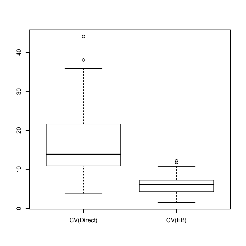
where πd​i\pi_{di} is the inclusion probability of ii-th unit in the sample from municipality dd. The sampling variance is obtained using the following approximation for the second-order inclusion probabilities πd,i​j≈πd​i​πd​j\pi_{d,ij}\approx\pi_{di}\pi_{dj}, j≠ij\neq i, and noting that πd,i​i=πd​i\pi_{d,ii}=\pi_{di} for all ii. Figure shows EB, direct, Molina (2009) and naive estimators of mean income for the D=57D=57 municipalities. This figure illustrates that direct estimators are somewhat unstable. According to Proposition 1, Molina (2009) and naive estimators have an average estimated relative bias of -14.77% and -14.92% respectively. In this application, both take very similar values (superposed in the plot) and their values are lower than those of EB estimators, which could be due to the mentioned theoretical bias.

Finally, boxplots of the estimated coefficients of variation (CVs) defined for any estimator τ^d\hat{\tau}_{d} as cv​(τ^d)=100×var​(τ^d)/τ^d\mbox{cv}(\hat{\tau}_{d})=100\times\sqrt{\mbox{var}(\hat{\tau}_{d})}/\hat{\tau}_{d} are shown in Figure 3. These boxplots show the significant reduction in CV obtained when using EB estimators instead of the default direct estimators.

Refer to caption

Refer to caption

Figure 3: EB, Molina (2009), naive and direct estimates of mean income for each municipality (left) and boxplots of estimated CVs of direct and EB estimates of mean income (right).

APPENDIX: PROOFS

In this appendix, the Euclidean norm of a vector 𝐚{\mathbf{a}} is denoted by |𝐚|=(𝐚′​𝐚)1/2|{\mathbf{a}}|=({\mathbf{a}}^{\prime}{\mathbf{a}})^{1/2}. For a matrix AA, we consider the norms ‖A‖=λmax1/2​(A′​A)\|A\|=\lambda_{\max}^{1/2}(A^{\prime}A) and ‖A‖2=tr1/2​(A′​A)\|A\|_{2}=\mbox{tr}^{1/2}(A^{\prime}A), where λmax​(A)\lambda_{\max}(A) denotes the maximum eigenvalue of AA. Asymptotic orders refer to D→∞D\to\infty.

PROOF OF PROPOSITION 1

The naive predictor of wd​iw_{di} can be expressed in terms of the best predictor w~d​i\tilde{w}_{di} as w~d​iN=exp⁡(y~d​i)=exp⁡(−αd)​w~d​i\tilde{w}_{di}^{N}=\exp(\tilde{y}_{di})=\exp(-\alpha_{d})\tilde{w}_{di}. Now since the best predictor w~d​i\tilde{w}_{di} is unbiased, that is, E⁡(w~d​i)=E⁡(wd​i)E(\tilde{w}_{di})=E(w_{di}), we have E⁡(w~d​iN)=exp⁡(−αd)​E​(w~d​i)=exp⁡(−αd)​E​(wd​i)E(\tilde{w}_{di}^{N})=\exp(-\alpha_{d})E(\tilde{w}_{di})=\exp(-\alpha_{d})E(w_{di}). The relative bias (RB) of w~d​iN\tilde{w}_{di}^{N} is then R​B​(w~d​iN)=E⁡(w~d​iN)/E⁡(wd​i)−1=exp⁡(−αd)−1RB(\tilde{w}_{di}^{N})=E(\tilde{w}_{di}^{N})/E(w_{di})-1=\exp(-\alpha_{d})-1. Similarly, Molina (2009) predictor can be expressed as w~d​iN=exp(y~d​i+αdM)=exp(−σe2/2)w~d​i\tilde{w}_{di}^{N}=\exp(\tilde{y}_{di}+\alpha_{d}^{M})=\exp(-\sigma_{e}^{2}/2)\tilde{w}_{di}. Taking expected value, we get E(w~d​iM)=exp(−σe2/2)E(wd​i)E(\tilde{w}_{di}^{M})=\exp(-\sigma_{e}^{2}/2)E(w_{di}). Thus, RB(w~d​iM)=E(w~d​iM)/E(wd​i)−1=exp(−σe2/2)−1RB(\tilde{w}_{di}^{M})=E(\tilde{w}_{di}^{M})/E(w_{di})-1=\exp(-\sigma_{e}^{2}/2)-1. □\Box

The next lemma is required in the proofs of several of the remaining results.

Lemma 1.

Let 𝐕s{\mathbf{V}}_{s} be the covariance matrix of 𝐲s{\mathbf{y}}_{s}, ℱ{\cal F} and ℱR{\cal F}_{R} the ML and REML Fisher-information matrices respectively, and 𝐐s=(𝐗s′​𝐕s−1​𝐗s)−1{\mathbf{Q}}_{s}=({\mathbf{X}}_{s}^{\prime}{\mathbf{V}}_{s}^{-1}{\mathbf{X}}_{s})^{-1}. It holds

  • (i)

    Condition (H1) implies ‖𝐕s‖=O⁡(1)\|{\mathbf{V}}_{s}\|=O(1).

  • (ii)

    ‖𝐕s−1‖=O⁡(1)\|{\mathbf{V}}_{s}^{-1}\|=O(1).

  • (iii)

    Conditions (H1) and (H3) imply ‖𝐐s‖=O⁡(D−1)\|{\mathbf{Q}}_{s}\|=O(D^{-1}).

  • (iv)

    Condition (H4) implies ‖ℱ−1‖=O⁡(D−1)\|{\cal F}^{-1}\|=O(D^{-1}) and ‖ℱR−1‖=O⁡(D−1)\|{\cal F}_{R}^{-1}\|=O(D^{-1}).

PROOF OF LEMMA 1

(i) Since 𝐕s{\mathbf{V}}_{s} is symmetric and block-diagonal with blocks equal to 𝐕d​s{\mathbf{V}}_{ds}, d=1,…,Dd=1,\ldots,D, we have

‖𝐕s‖=λmax1/2​(𝐕s2)=λmax​(𝐕s)=max1≤d≤D⁡{λmax​(𝐕d​s)}.\|{\mathbf{V}}_{s}\|=\lambda_{\max}^{1/2}({\mathbf{V}}_{s}^{2})=\lambda_{\max}({\mathbf{V}}_{s})=\max_{1\leq d\leq D}\{\lambda_{\max}({\mathbf{V}}_{ds})\}.

Now since 𝐕d​s=σu2​𝟏nd​𝟏nd′+σe2​𝐈nd{\mathbf{V}}_{ds}=\sigma_{u}^{2}\mathbf{1}_{n_{d}}\mathbf{1}_{n_{d}}^{\prime}+\sigma_{e}^{2}{\mathbf{I}}_{n_{d}}, we have

λmax​(𝐕d)≤σu2​λmax​(𝟏nd​𝟏nd′)+σe2​λmax​(𝐈nd)=σu2​nd+σe2.\lambda_{\max}({\mathbf{V}}_{d})\leq\sigma_{u}^{2}\lambda_{\max}(\mathbf{1}_{n_{d}}\mathbf{1}_{n_{d}}^{\prime})+\sigma_{e}^{2}\lambda_{\max}({\mathbf{I}}_{n_{d}})=\sigma_{u}^{2}n_{d}+\sigma_{e}^{2}.

Then, by assumption (H1), we obtain

‖𝐕s‖=max1≤d≤D⁡{λmax​(𝐕d​s)}≤σu2​max1≤d≤D​nd+σe2=O⁡(1),\|{\mathbf{V}}_{s}\|=\max_{1\leq d\leq D}\{\lambda_{\max}({\mathbf{V}}_{ds})\}\leq\sigma_{u}^{2}\max_{1\leq d\leq D}n_{d}+\sigma_{e}^{2}=O(1),

which implies (i). □\Box
(ii) Similarly as before, we have

‖𝐕s−1‖=λmax​(𝐕s−1)=λmin−1​(𝐕s)={min1≤d≤D⁡λmin​(𝐕d​s)}−1.\|{\mathbf{V}}_{s}^{-1}\|=\lambda_{\max}({\mathbf{V}}_{s}^{-1})=\lambda_{\min}^{-1}({\mathbf{V}}_{s})=\left\{\min_{1\leq d\leq D}\lambda_{\min}({\mathbf{V}}_{ds})\right\}^{-1}.

But again, using the expression of 𝐕d​s=σu2​𝟏nd​𝟏nd′+σe2​𝐈nd{\mathbf{V}}_{ds}=\sigma_{u}^{2}\mathbf{1}_{n_{d}}\mathbf{1}_{n_{d}}^{\prime}+\sigma_{e}^{2}{\mathbf{I}}_{n_{d}}, we have

λmin​(𝐕d)≥σu2​λmin​(𝟏nd​𝟏nd′)+σe2​λmin​(𝐈nd)=σe2>0,\lambda_{\min}({\mathbf{V}}_{d})\geq\sigma_{u}^{2}\lambda_{\min}(\mathbf{1}_{n_{d}}\mathbf{1}_{n_{d}}^{\prime})+\sigma_{e}^{2}\lambda_{\min}({\mathbf{I}}_{n_{d}})=\sigma_{e}^{2}>0,

which is true for all d∈{1,…,D}d\in\{1,\ldots,D\} and for all DD. Therefore, ‖𝐕s−1‖=O⁡(1)\|{\mathbf{V}}_{s}^{-1}\|=O(1). □\Box
(iii) By the definition of 𝐐s=(𝐗s′​𝐕s−1​𝐗s)−1{\mathbf{Q}}_{s}=({\mathbf{X}}_{s}^{\prime}{\mathbf{V}}_{s}^{-1}{\mathbf{X}}_{s})^{-1}, we obtain

‖𝐐s‖=λmax​(𝐐s)=λmin−1​(𝐗s′​𝐕s−1​𝐗s).\|{\mathbf{Q}}_{s}\|=\lambda_{\max}({\mathbf{Q}}_{s})=\lambda_{\min}^{-1}({\mathbf{X}}_{s}^{\prime}{\mathbf{V}}_{s}^{-1}{\mathbf{X}}_{s}).

But by the definition of eigenvalue, we have

λmin​(𝐗s′​𝐕s−1​𝐗s)=minv⁡v′​𝐗s′​𝐕s−1​𝐗s​vv′​v=minv⁡(v′​𝐗s′​𝐕s−1​𝐗s​vv′​𝐗s′​𝐗s​v​v′​𝐗s′​𝐗s​vv′​v)\displaystyle\lambda_{\min}({\mathbf{X}}_{s}^{\prime}{\mathbf{V}}_{s}^{-1}{\mathbf{X}}_{s})=\min_{v}\frac{v^{\prime}{\mathbf{X}}_{s}^{\prime}{\mathbf{V}}_{s}^{-1}{\mathbf{X}}_{s}v}{v^{\prime}v}=\min_{v}\left(\frac{v^{\prime}{\mathbf{X}}_{s}^{\prime}{\mathbf{V}}_{s}^{-1}{\mathbf{X}}_{s}v}{v^{\prime}{\mathbf{X}}_{s}^{\prime}{\mathbf{X}}_{s}v}\frac{v^{\prime}{\mathbf{X}}_{s}^{\prime}{\mathbf{X}}_{s}v}{v^{\prime}v}\right)
≥(minw⁡w′​𝐗s′​𝐕s−1​𝐗s​ww′​𝐗s′​𝐗s​w)​(minv⁡v′​𝐗s′​𝐗s​vv′​v)=λmin​(𝐕s−1)​λmin​(𝐗s′​𝐗s)\displaystyle\geq\left(\min_{w}\frac{w^{\prime}{\mathbf{X}}_{s}^{\prime}{\mathbf{V}}_{s}^{-1}{\mathbf{X}}_{s}w}{w^{\prime}{\mathbf{X}}_{s}^{\prime}{\mathbf{X}}_{s}w}\right)\left(\min_{v}\frac{v^{\prime}{\mathbf{X}}_{s}^{\prime}{\mathbf{X}}_{s}v}{v^{\prime}v}\right)=\lambda_{\min}({\mathbf{V}}_{s}^{-1})\lambda_{\min}({\mathbf{X}}_{s}^{\prime}{\mathbf{X}}_{s})
=λmax−1​(𝐕s)​λmin​(𝐗s′​𝐗s).\displaystyle=\lambda_{\max}^{-1}({\mathbf{V}}_{s})\lambda_{\min}({\mathbf{X}}_{s}^{\prime}{\mathbf{X}}_{s}).

Using (i) and assumption (H3), we finally get

D​‖𝐐s‖=D​λmin−1​(𝐗s′​𝐕s−1​𝐗s)≤λmax​(𝐕s)D−1​λmin​(𝐗s′​𝐗s)=O⁡(1),D\|{\mathbf{Q}}_{s}\|=D\lambda_{\min}^{-1}({\mathbf{X}}_{s}^{\prime}{\mathbf{V}}_{s}^{-1}{\mathbf{X}}_{s})\leq\frac{\lambda_{\max}({\mathbf{V}}_{s})}{D^{-1}\lambda_{\min}({\mathbf{X}}_{s}^{\prime}{\mathbf{X}}_{s})}=O(1),

which means that ‖𝐐s‖=O⁡(D−1)\|{\mathbf{Q}}_{s}\|=O(D^{-1}). □\Box
(iv) Condition (H4) implies

D​‖ℱ−1‖=D​λmax​(ℱ−1)=1D−1​λmin​(ℱ)=O⁡(1),D\|{\cal F}^{-1}\|=D\lambda_{\max}({\cal F}^{-1})=\frac{1}{D^{-1}\lambda_{\min}({\cal F})}=O(1),

which is equivalent to ‖ℱ−1‖=O⁡(D−1)\|{\cal F}^{-1}\|=O(D^{-1}). Moreover, note that ℱ=−A/2+B{\cal F}=-A/2+B, where B=(bh​ℓ)h,ℓ=1,2B=(b_{h\ell})_{h,\ell=1,2} and A=(ah​ℓ)h,ℓ=1,2A=(a_{h\ell})_{h,\ell=1,2}, for ah​ℓ=tr​(𝐕s−1​𝚫h​𝐕s−1​𝚫ℓ)a_{h\ell}=\mbox{tr}({\mathbf{V}}_{s}^{-1}\bm{\Delta}_{h}{\mathbf{V}}_{s}^{-1}\bm{\Delta}_{\ell}) and bh​ℓ=tr​(𝐏s​𝚫h​𝐏s​𝚫ℓ)b_{h\ell}=\mbox{tr}({\mathbf{P}}_{s}\bm{\Delta}_{h}{\mathbf{P}}_{s}\bm{\Delta}_{\ell}), whereas ℱR=B/2{\cal F}_{R}=B/2. Then,

λmin​(ℱR)\displaystyle\lambda_{\min}({\cal F}_{R}) =\displaystyle= λmin​(B−B/2)=λmin​(B−B/2+A/2−A/2)\displaystyle\lambda_{\min}\left(B-B/2\right)=\lambda_{\min}\left(B-B/2+A/2-A/2\right)
=\displaystyle= λmin​{ℱ+(A−B)/2}≥λmin​(ℱ)+12​λmin​(A−B).\displaystyle\lambda_{\min}\left\{{\cal F}+(A-B)/2\right\}\geq\lambda_{\min}({\cal F})+\frac{1}{2}\lambda_{\min}(A-B).

But the diagonal elements of D−1​(A−B)D^{-1}(A-B) tend to zero. Indeed

bh​h−ah​h\displaystyle b_{hh}-a_{hh} =\displaystyle= tr​(𝐏s​𝚫h​𝐏s​𝚫h)−tr​(𝐕s−1​𝚫h​𝐕s−1​𝚫h)\displaystyle\mbox{tr}({\mathbf{P}}_{s}\bm{\Delta}_{h}{\mathbf{P}}_{s}\bm{\Delta}_{h})-\mbox{tr}({\mathbf{V}}_{s}^{-1}\bm{\Delta}_{h}{\mathbf{V}}_{s}^{-1}\bm{\Delta}_{h})
=\displaystyle= tr​(𝐏s​𝚫h​𝐖s​𝚫h)+tr​(𝐖s​𝚫h​𝐕s−1​𝚫h),\displaystyle\mbox{tr}({\mathbf{P}}_{s}\bm{\Delta}_{h}{\mathbf{W}}_{s}\bm{\Delta}_{h})+\mbox{tr}({\mathbf{W}}_{s}\bm{\Delta}_{h}{\mathbf{V}}_{s}^{-1}\bm{\Delta}_{h}),

for 𝐖s=𝐏s−𝐕s−1=𝐕s−1​𝐗s​(𝐗s′​𝐕s−1​𝐗s)−1​𝐗s′​𝐕s−1{\mathbf{W}}_{s}={\mathbf{P}}_{s}-{\mathbf{V}}_{s}^{-1}={\mathbf{V}}_{s}^{-1}{\mathbf{X}}_{s}({\mathbf{X}}_{s}^{\prime}{\mathbf{V}}_{s}^{-1}{\mathbf{X}}_{s})^{-1}{\mathbf{X}}_{s}^{\prime}{\mathbf{V}}_{s}^{-1}. Then,

|bh​h−ah​h|≤|tr​(𝐏s​𝚫h​𝐖s​𝚫h)|+|tr​(𝐖s​𝚫h​𝐕s−1​𝚫h)|.|b_{hh}-a_{hh}|\leq|\mbox{tr}({\mathbf{P}}_{s}\bm{\Delta}_{h}{\mathbf{W}}_{s}\bm{\Delta}_{h})|+|\mbox{tr}({\mathbf{W}}_{s}\bm{\Delta}_{h}{\mathbf{V}}_{s}^{-1}\bm{\Delta}_{h})|.

Now, for the second term on the right-hand side, we have

|tr​(𝐖s​𝚫h​𝐕s−1​𝚫h)|=|tr​(𝐕s−1​𝐗s​(𝐗s′​𝐕s−1​𝐗s)−1​𝐗s​𝐕s−1​𝚫h​𝐕s−1​𝚫h)|\displaystyle|\mbox{tr}({\mathbf{W}}_{s}\bm{\Delta}_{h}{\mathbf{V}}_{s}^{-1}\bm{\Delta}_{h})|=|\mbox{tr}({\mathbf{V}}_{s}^{-1}{\mathbf{X}}_{s}({\mathbf{X}}_{s}^{\prime}{\mathbf{V}}_{s}^{-1}{\mathbf{X}}_{s})^{-1}{\mathbf{X}}_{s}{\mathbf{V}}_{s}^{-1}\bm{\Delta}_{h}{\mathbf{V}}_{s}^{-1}\bm{\Delta}_{h})|
=|tr{(𝐗s′𝐕s−1𝐗s)−1/2𝐗s𝐕s−1𝚫h𝐕s−1𝚫h𝐕s−1𝐗s(𝐗s′𝐕s−1𝐗s)−1/2}|\displaystyle=|\mbox{tr}\{({\mathbf{X}}_{s}^{\prime}{\mathbf{V}}_{s}^{-1}{\mathbf{X}}_{s})^{-1/2}{\mathbf{X}}_{s}{\mathbf{V}}_{s}^{-1}\bm{\Delta}_{h}{\mathbf{V}}_{s}^{-1}\bm{\Delta}_{h}{\mathbf{V}}_{s}^{-1}{\mathbf{X}}_{s}({\mathbf{X}}_{s}^{\prime}{\mathbf{V}}_{s}^{-1}{\mathbf{X}}_{s})^{-1/2}\}|
≤pλmax{(𝐗s′𝐕s−1𝐗s)−1/2𝐗s𝐕s−1𝚫h𝐕s−1𝚫h𝐕s−1𝐗s(𝐗s′𝐕s−1𝐗s)−1/2}\displaystyle\leq p\lambda_{\max}\{({\mathbf{X}}_{s}^{\prime}{\mathbf{V}}_{s}^{-1}{\mathbf{X}}_{s})^{-1/2}{\mathbf{X}}_{s}{\mathbf{V}}_{s}^{-1}\bm{\Delta}_{h}{\mathbf{V}}_{s}^{-1}\bm{\Delta}_{h}{\mathbf{V}}_{s}^{-1}{\mathbf{X}}_{s}({\mathbf{X}}_{s}^{\prime}{\mathbf{V}}_{s}^{-1}{\mathbf{X}}_{s})^{-1/2}\}
=p∥𝐕s−1/2𝚫h𝐕s−1𝐗s(𝐗s′𝐕s−1𝐗s)−1/2∥2\displaystyle=p\|{\mathbf{V}}_{s}^{-1/2}\bm{\Delta}_{h}{\mathbf{V}}_{s}^{-1}{\mathbf{X}}_{s}({\mathbf{X}}_{s}^{\prime}{\mathbf{V}}_{s}^{-1}{\mathbf{X}}_{s})^{-1/2}\|^{2}
≤pλmin−4(𝐕s)∥𝚫h∥2∥𝐕s−1/2𝐗s(𝐗s′𝐕s−1𝐗s)−1/2∥2\displaystyle\leq p\lambda_{\min}^{-4}({\mathbf{V}}_{s})\|\bm{\Delta}_{h}\|^{2}\|{\mathbf{V}}_{s}^{-1/2}{\mathbf{X}}_{s}({\mathbf{X}}_{s}^{\prime}{\mathbf{V}}_{s}^{-1}{\mathbf{X}}_{s})^{-1/2}\|^{2}
=p​λmin−4​(𝐕s)​‖𝚫h‖2=O⁡(1).\displaystyle=p\lambda_{\min}^{-4}({\mathbf{V}}_{s})\|\bm{\Delta}_{h}\|^{2}=O(1).

Similarly, it is easy to see that |tr​(𝐏s​𝚫h​𝐖s​𝚫h)|=O⁡(1)|\mbox{tr}({\mathbf{P}}_{s}\bm{\Delta}_{h}{\mathbf{W}}_{s}\bm{\Delta}_{h})|=O(1). Therefore, it holds that D−1​(ah​h−bh​h)→0D^{-1}(a_{hh}-b_{hh})\to 0 as D→∞D\to\infty for h=1,2h=1,2, leading to limD→∞λmin​{D−1​(A−B)}=lim infλmin​{D−1​(A−B)}=0\lim_{D\to\infty}\lambda_{\min}\{D^{-1}(A-B)\}=\liminf\lambda_{\min}\{D^{-1}(A-B)\}=0, which in turn implies

lim infD−1​λmin​(ℱR)≥lim infD−1​λmin​(ℱ)+lim infλmin​{D−1​(A−B)}>0.\liminf D^{-1}\lambda_{\min}({\cal F}_{R})\geq\liminf D^{-1}\lambda_{\min}({\cal F})+\liminf\lambda_{\min}\{D^{-1}(A-B)\}>0.

Then, similarly as we did for ℱ{\cal F} above, we obtain ‖ℱR−1‖=O⁡(D−1)\|{\cal F}_{R}^{-1}\|=O(D^{-1}). □\Box

PROOF OF PROPOSITION 2

First of all, note that

E⁡(wd​i)=E⁡[exp⁡(yd​i)]=exp⁡{𝐱d​i′​𝜷+(σu2+σe2)/2}.E(w_{di})=E[\exp(y_{di})]=\exp\{{\mathbf{x}}_{di}^{\prime}\bm{\beta}+(\sigma_{u}^{2}+\sigma_{e}^{2})/2\}. (27)

On the other hand, w^d​i=exp⁡(y^d​i+αd)\hat{w}_{di}=\exp(\hat{y}_{di}+\alpha_{d}), where y^d​i\hat{y}_{di} is given by

y^d​i=𝐛d​i′​𝐲s,\hat{y}_{di}={\mathbf{b}}_{di}^{\prime}{\mathbf{y}}_{s}, (28)

for the vector

𝐛d​i=𝐕s−1​𝐗s​𝐐s​𝐱d​i+σu2​𝐏s​𝐙s​𝐦d,{\mathbf{b}}_{di}={\mathbf{V}}_{s}^{-1}{\mathbf{X}}_{s}{\mathbf{Q}}_{s}{\mathbf{x}}_{di}+\sigma_{u}^{2}{\mathbf{P}}_{s}{\mathbf{Z}}_{s}{\mathbf{m}}_{d}, (29)

where 𝐦d=(𝟎d−1′,1,𝟎D−d′)′{\mathbf{m}}_{d}=(\mathbf{0}_{d-1}^{\prime},1,\mathbf{0}_{D-d}^{\prime})^{\prime}. Replacing 𝐲s=𝐗s​𝜷+𝐯s{\mathbf{y}}_{s}={\mathbf{X}}_{s}\bm{\beta}+{\mathbf{v}}_{s}, for 𝐯s=𝐙s​𝐮+𝐞s{\mathbf{v}}_{s}={\mathbf{Z}}_{s}{\mathbf{u}}+{\mathbf{e}}_{s} in (28) and noting that 𝐛d​i′​𝐗s​𝜷=𝐱d​i′​𝜷{\mathbf{b}}_{di}^{\prime}{\mathbf{X}}_{s}\bm{\beta}={\mathbf{x}}_{di}^{\prime}\bm{\beta} because 𝐏s​𝐗s=𝟎n{\mathbf{P}}_{s}{\mathbf{X}}_{s}=\mathbf{0}_{n}, we obtain y^d​i=𝐱d​i′​𝜷+𝐛d​i′​𝐯s\hat{y}_{di}={\mathbf{x}}_{di}^{\prime}\bm{\beta}+{\mathbf{b}}_{di}^{\prime}{\mathbf{v}}_{s}. Hence, the first-stage EB predictor of wd​iw_{di} can be expressed as

w^d​i=exp⁡(y^d​i+αd),y^d​i=𝐱d​i′​𝜷+𝐛d​i′​𝐯s.\hat{w}_{di}=\exp(\hat{y}_{di}+\alpha_{d}),\quad\hat{y}_{di}={\mathbf{x}}_{di}^{\prime}\bm{\beta}+{\mathbf{b}}_{di}^{\prime}{\mathbf{v}}_{s}. (30)

Taking expected value, we get

E⁡(w^d​i)=exp⁡(𝐱d​i′​𝜷+αd+𝐛d​i′​𝐕s​𝐛d​i/2).E(\hat{w}_{di})=\exp\left({\mathbf{x}}_{di}^{\prime}\bm{\beta}+\alpha_{d}+{\mathbf{b}}_{di}^{\prime}{\mathbf{V}}_{s}{\mathbf{b}}_{di}/2\right). (31)

Using the definition of 𝐛d​i{\mathbf{b}}_{di} in (29) and 𝐏s{\mathbf{P}}_{s} in (11) and taking into account that 𝐗s′​𝐏s=𝟎p×n{\mathbf{X}}_{s}^{\prime}{\mathbf{P}}_{s}=\mathbf{0}_{p\times n} and 𝐏s​𝐕s​𝐏s=𝐏s{\mathbf{P}}_{s}{\mathbf{V}}_{s}{\mathbf{P}}_{s}={\mathbf{P}}_{s}, it is easy to see that

𝐛d​i′​𝐕s​𝐛d​i=𝐱d​i′​𝐐s​𝐱d​i+(σu2)2​𝐦d′​𝐙s′​𝐕s−1​𝐙s​𝐦d−(σu2)2​𝐦d′​𝐙s′​𝐕s−1​𝐗s​𝐐s​𝐗s′​𝐕s−1​𝐙s​𝐦d.{\mathbf{b}}_{di}^{\prime}{\mathbf{V}}_{s}{\mathbf{b}}_{di}={\mathbf{x}}_{di}^{\prime}{\mathbf{Q}}_{s}{\mathbf{x}}_{di}+(\sigma_{u}^{2})^{2}{\mathbf{m}}_{d}^{\prime}{\mathbf{Z}}_{s}^{\prime}{\mathbf{V}}_{s}^{-1}{\mathbf{Z}}_{s}{\mathbf{m}}_{d}-(\sigma_{u}^{2})^{2}{\mathbf{m}}_{d}^{\prime}{\mathbf{Z}}_{s}^{\prime}{\mathbf{V}}_{s}^{-1}{\mathbf{X}}_{s}{\mathbf{Q}}_{s}{\mathbf{X}}_{s}^{\prime}{\mathbf{V}}_{s}^{-1}{\mathbf{Z}}_{s}{\mathbf{m}}_{d}. (32)

Since 𝐕s=diag1≤d≤D​(𝐕d​s){\mathbf{V}}_{s}=\mbox{diag}_{1\leq d\leq D}({\mathbf{V}}_{ds}) with 𝐕d​s=σu2​𝟏nd​𝟏nd′+σe2​𝐈nd{\mathbf{V}}_{ds}=\sigma_{u}^{2}\mathbf{1}_{n_{d}}\mathbf{1}_{n_{d}}^{\prime}+\sigma_{e}^{2}{\mathbf{I}}_{n_{d}}, 𝐦d=(𝟎d−1′,1,𝟎D−d′)′{\mathbf{m}}_{d}=(\mathbf{0}_{d-1}^{\prime},1,\mathbf{0}_{D-d}^{\prime})^{\prime}, 𝐙d​s=diag1≤d≤D​(𝟏nd){\mathbf{Z}}_{ds}=\mbox{diag}_{1\leq d\leq D}(\mathbf{1}_{n_{d}}) and 𝐗s=(𝐗1​s′,…,𝐗D​s′)′{\mathbf{X}}_{s}=({\mathbf{X}}_{1s}^{\prime},\ldots,{\mathbf{X}}_{Ds}^{\prime})^{\prime}, we obtain

𝐦d′​𝐙s′​𝐕s−1​𝐙s​𝐦d=γd/σu2,𝐦d′​𝐙s′​𝐕s−1​𝐗s=(γd/σu2)​𝐱¯d​s′.{\mathbf{m}}_{d}^{\prime}{\mathbf{Z}}_{s}^{\prime}{\mathbf{V}}_{s}^{-1}{\mathbf{Z}}_{s}{\mathbf{m}}_{d}=\gamma_{d}/\sigma_{u}^{2},\quad{\mathbf{m}}_{d}^{\prime}{\mathbf{Z}}_{s}^{\prime}{\mathbf{V}}_{s}^{-1}{\mathbf{X}}_{s}=(\gamma_{d}/\sigma_{u}^{2})\bar{{\mathbf{x}}}_{ds}^{\prime}. (33)

Replacing (33) in (32), we finally obtain

𝐛d​i′​𝐕s​𝐛d​i=𝐱d​i′​𝐐s​𝐱d​i+γd​(σu2−γd​𝐱¯d​s′​𝐐s​𝐱¯d​s)=γd​σu2+hd,i​i−γd2​hd,{\mathbf{b}}_{di}^{\prime}{\mathbf{V}}_{s}{\mathbf{b}}_{di}={\mathbf{x}}_{di}^{\prime}{\mathbf{Q}}_{s}{\mathbf{x}}_{di}+\gamma_{d}(\sigma_{u}^{2}-\gamma_{d}\bar{\mathbf{x}}_{ds}^{\prime}{\mathbf{Q}}_{s}\bar{\mathbf{x}}_{ds})=\gamma_{d}\sigma_{u}^{2}+h_{d,ii}-\gamma_{d}^{2}h_{d}, (34)

for hd,i​i=𝐱d​i′​𝐐s​𝐱d​ih_{d,ii}={\mathbf{x}}_{di}^{\prime}{\mathbf{Q}}_{s}{\mathbf{x}}_{di} and hd=𝐱¯d′​𝐐s​𝐱dh_{d}=\bar{\mathbf{x}}_{d}^{\prime}{\mathbf{Q}}_{s}{\mathbf{x}}_{d}. Replacing (34) in (31), we obtain

E⁡(w^d​i)=exp⁡{𝐱d​i′​𝜷+(σu2+σe2)/2+(hd,i​i−γd2​hd)/2}.E(\hat{w}_{di})=\exp\left\{{\mathbf{x}}_{di}^{\prime}\bm{\beta}+(\sigma_{u}^{2}+\sigma_{e}^{2})/2+(h_{d,ii}-\gamma_{d}^{2}h_{d})/2\right\}.

Finally, by Lemma 1, under (H1) and (H3), we have ‖𝐐s‖=O⁡(D−1)\|{\mathbf{Q}}_{s}\|=O(D^{-1}), and using (H2), it holds |hd,i​i|=O⁡(D−1)|h_{d,ii}|=O(D^{-1}) and |hd|=O⁡(D−1)|h_{d}|=O(D^{-1}). The result then follows by (28). □\Box

PROOF OF THEOREM 1

(i) The best predictor of wd​i=exp⁡(yd​i)w_{di}=\exp(y_{di}) is equal to w~d​i=E𝐲d​r​{exp⁡(yd​i)|𝐲d​s}\tilde{w}_{di}=E_{{\mathbf{y}}_{dr}}\{\exp(y_{di})|{\mathbf{y}}_{ds}\}. Here we calculate the more general expectation E𝐲d​r​{exp⁡(𝐲d​r′​𝐛d)|𝐲d​s}E_{{\mathbf{y}}_{dr}}\left\{\exp({\mathbf{y}}_{dr}^{\prime}{\mathbf{b}}_{d})|{\mathbf{y}}_{ds}\right\}, where 𝐛d{\mathbf{b}}_{d} is a non-stochastic vector of size Nd−ndN_{d}-n_{d}, d=1,…,Dd=1,\ldots,D. Now using the conditional distribution given in (3), this expectation is given by

E𝐲d​r​[exp⁡(𝐲d​r′​𝐛d)|𝐲d​s]=exp⁡(𝝁d​r|s′​𝐛d+12​𝐛d′​𝐕d​r|s​𝐛d),E_{{\mathbf{y}}_{dr}}\left[\exp\left({\mathbf{y}}_{dr}^{\prime}{\mathbf{b}}_{d}\right)|{\mathbf{y}}_{ds}\right]=\exp\left(\bm{\mu}_{dr|s}^{\prime}{\mathbf{b}}_{d}+\frac{1}{2}\,{\mathbf{b}}_{d}^{\prime}{\mathbf{V}}_{dr|s}{\mathbf{b}}_{d}\right), (35)

because the integral involved is equal to 1. Now (i) follows from the expressions for 𝝁d​r|s\bm{\mu}_{dr|s} and 𝐕d​r|s{\mathbf{V}}_{dr|s} given in (4) and (5), and taking 𝐛d{\mathbf{b}}_{d} as a vector with 1 in position ii and the rest of elements equal to zero.
(ii) The best predictor of τd\tau_{d} is given by

τ~d=τ~d​(𝜷,𝜽)=E𝐲d​r​(τd|𝐲d​s)=1Nd​[∑i∈sdexp⁡(yd​i)+∑i∈s¯dE𝐲d​r​{exp⁡(yd​i)|𝐲d​s}].\tilde{\tau}_{d}=\tilde{\tau}_{d}(\bm{\beta},\bm{\theta})=E_{{\mathbf{y}}_{dr}}\left(\tau_{d}|{\mathbf{y}}_{ds}\right)=\frac{1}{N_{d}}\left[\sum_{i\in s_{d}}\exp(y_{di})+\sum_{i\in\bar{s}_{d}}E_{{\mathbf{y}}_{dr}}\left\{\exp(y_{di})|{\mathbf{y}}_{ds}\right\}\right]. (36)

The result then follows by straightforward application of (i). □\Box

PROOF OF THEOREM 2

For i,j∈s¯di,j\in\bar{s}_{d}, we need to calculate

MCPE​(w~d​i,w~d​j)=E⁡(w~d​i​w~d​j)−E⁡(w~d​i​wd​j)−E⁡(wd​i​w~d​j)+E⁡(wd​i​wd​j).\mbox{MCPE}(\tilde{w}_{di},\tilde{w}_{dj})=E(\tilde{w}_{di}\tilde{w}_{dj})-E(\tilde{w}_{di}w_{dj})-E(w_{di}\tilde{w}_{dj})+E(w_{di}w_{dj}). (37)

Since udu_{d} and ed​ie_{di} are independent for all ii, the last term on the right hand side of (37) for i≠ji\neq j is given by

E⁡(wd​i​wd​j)=exp⁡{(𝐱d​i+𝐱d​j)′​𝜷}​E​{exp⁡(2​ud)}​E​{exp⁡(ed​i)}​E​{exp⁡(ed​j)}.E(w_{di}w_{dj})=\exp\left\{({\mathbf{x}}_{di}+{\mathbf{x}}_{dj})^{\prime}\bm{\beta}\right\}E\left\{\exp(2u_{d})\right\}E\left\{\exp(e_{di})\right\}E\left\{\exp(e_{dj})\right\}. (38)

In contrast, for i=ji=j we have

E⁡(wd​i2)=exp⁡(2​𝐱d​i′​𝜷)​E​{exp⁡(2​ud)}​E​{exp⁡(2​ed​i)}.E(w_{di}^{2})=\exp(2{\mathbf{x}}_{di}^{\prime}\bm{\beta})E\left\{\exp(2u_{d})\right\}E\left\{\exp(2e_{di})\right\}. (39)

Observe that the expectations appearing on the right hand side of (38) and (39) are respectively the moment generating function (m.g.f.) of the independent random variables 2​ud2u_{d}, ed​ie_{di}, ed​je_{dj} and 2​ed​i2e_{di}, evaluated at t=1t=1. Since the m.g.f. of a random variable X∼𝒩⁡(μ,σ2)X\sim{\cal N}(\mu,\sigma^{2}) is given by MX​(t)=exp⁡(μ​t+σ2​t2/2)M_{X}(t)=\exp(\mu t+\sigma^{2}t^{2}/2), using this expression we get

E(wd​iwd​j)=exp{(𝐱d​i+𝐱d​j)′𝜷+2σu2+σe2(1+1{i=j})}.E(w_{di}w_{dj})=\exp\left\{({\mathbf{x}}_{di}+{\mathbf{x}}_{dj})^{\prime}\bm{\beta}+2\sigma_{u}^{2}+\sigma_{e}^{2}(1+1_{\{i=j\}})\right\}. (40)

Now we obtain E⁡(w~d​i​wd​j)=E⁡{exp⁡(y~d​i+αd+yd​j)}E(\tilde{w}_{di}w_{dj})=E\left\{\exp(\tilde{y}_{di}+\alpha_{d}+y_{dj})\right\}. But by model (1), we know

yd​j=𝐱d​j′​𝜷+ud+ed​j,\displaystyle y_{dj}={\mathbf{x}}_{dj}^{\prime}\bm{\beta}+u_{d}+e_{dj},
y~d​i=𝐱d​i′​𝜷+γd​(y¯d​s−𝐱¯d​s′​𝜷)=𝐱d​i′​𝜷+γd​(ud+e¯d​s),\displaystyle\tilde{y}_{di}={\mathbf{x}}_{di}^{\prime}\bm{\beta}+\gamma_{d}(\bar{y}_{ds}-\bar{{\mathbf{x}}}_{ds}^{\prime}\bm{\beta})={\mathbf{x}}_{di}^{\prime}\bm{\beta}+\gamma_{d}(u_{d}+\bar{e}_{ds}),

Then,

y~d​i+yd​j=(𝐱d​i+𝐱d​j)′​𝜷+(1+γd)​ud+ed​j+γd​e¯d​s.\tilde{y}_{di}+y_{dj}=({\mathbf{x}}_{di}+{\mathbf{x}}_{dj})^{\prime}\bm{\beta}+(1+\gamma_{d})u_{d}+e_{dj}+\gamma_{d}\bar{e}_{ds}.

Noting that udu_{d}, ed​je_{dj} for j∈s¯dj\in\bar{s}_{d} and e¯d​s\bar{e}_{ds} are independent, we have

E⁡(w~d​i​wd​j)=E⁡{exp⁡(y~d​i+αd+yd​j)}\displaystyle E(\tilde{w}_{di}w_{dj})=E\left\{\exp(\tilde{y}_{di}+\alpha_{d}+y_{dj})\right\} (41)
=exp⁡{(𝐱d​i+𝐱d​j)′​𝜷}​exp⁡(αd)​E​[exp⁡{(1+γd)​ud}]​E​{exp⁡(ed​j)}​E​[exp⁡{γd​e¯d​s}].\displaystyle=\exp\{({\mathbf{x}}_{di}+{\mathbf{x}}_{dj})^{\prime}\bm{\beta}\}\exp(\alpha_{d})E\left[\exp\left\{(1+\gamma_{d})u_{d}\right\}\right]E\left\{\exp(e_{dj})\right\}E\left[\exp\left\{\gamma_{d}\bar{e}_{ds}\right\}\right].

Using the m.g.f.’s evaluated at t=1t=1 of the random variables involved in (41), using the expression of αd=12​{σu2​(1−γd)+σe2}\alpha_{d}=\frac{1}{2}\{\sigma_{u}^{2}(1-\gamma_{d})+\sigma_{e}^{2}\} and the fact that γd​(σu2+σe2/nd)=σu2\gamma_{d}(\sigma_{u}^{2}+\sigma_{e}^{2}/n_{d})=\sigma_{u}^{2}, we get

E(w~d​iwd​j)=exp{(𝐱d​i+𝐱d​j)′𝜷+2σu2+σe2−σu2(1−γd)=E(wd​iw~d​j)}.E(\tilde{w}_{di}w_{dj})=\exp\{({\mathbf{x}}_{di}+{\mathbf{x}}_{dj})^{\prime}\bm{\beta}+2\sigma_{u}^{2}+\sigma_{e}^{2}-\sigma_{u}^{2}(1-\gamma_{d})=E(w_{di}\tilde{w}_{dj})\}. (42)

Finally, we calculate E⁡(w~d​i​w~d​j)=E⁡{exp⁡(y~d​i+y~d​j+2​αd)}E(\tilde{w}_{di}\tilde{w}_{dj})=E\left\{\exp(\tilde{y}_{di}+\tilde{y}_{dj}+2\alpha_{d})\right\}. Again, by model (1), it holds

y~d​i+y~d​j=(𝐱d​i+𝐱d​j)′​𝜷+2​γd​(y¯d​s−𝐱¯d​s′​𝜷)=(𝐱d​i+𝐱d​j)′​𝜷+2​γd​(ud+e¯d​s).\tilde{y}_{di}+\tilde{y}_{dj}=({\mathbf{x}}_{di}+{\mathbf{x}}_{dj})^{\prime}\bm{\beta}+2\gamma_{d}(\bar{y}_{ds}-\bar{{\mathbf{x}}}_{ds}^{\prime}\bm{\beta})=({\mathbf{x}}_{di}+{\mathbf{x}}_{dj})^{\prime}\bm{\beta}+2\gamma_{d}(u_{d}+\bar{e}_{ds}).

Now since

2​γd​(ud+e¯d​s)∼𝒩⁡{0,4​γd2​(σu2+σe2nd)}≡𝒩⁡(0,4​γd​σu2),2\gamma_{d}(u_{d}+\bar{e}_{ds})\sim{\cal N}\left\{0,4\gamma_{d}^{2}\left(\sigma_{u}^{2}+\frac{\sigma_{e}^{2}}{n_{d}}\right)\right\}\equiv{\cal N}(0,4\gamma_{d}\,\sigma_{u}^{2}),

then using again the m.g.f. of γd​(ud+e¯d​s)\gamma_{d}(u_{d}+\bar{e}_{ds}) evaluated at t=1t=1, we get

E⁡[exp⁡{2​γd​(ud+e¯d​s)}]=exp⁡(2​γd​σu2).E\left[\exp\{2\gamma_{d}(u_{d}+\bar{e}_{ds})\}\right]=\exp(2\gamma_{d}\,\sigma_{u}^{2}).

Finally, using the expression of αd={σu2​(1−γd)+σe2}/2\alpha_{d}=\{\sigma_{u}^{2}(1-\gamma_{d})+\sigma_{e}^{2}\}/2, we get

E⁡(w~d​i​w~d​j)=exp⁡{(𝐱d​i+𝐱d​j)′​𝜷}​exp​{2​σu2+σe2−σu2​(1−γd)}=E⁡(w~d​i​wd​j).E(\tilde{w}_{di}\tilde{w}_{dj})=\exp\{({\mathbf{x}}_{di}+{\mathbf{x}}_{dj})^{\prime}\bm{\beta}\}\exp\{2\sigma_{u}^{2}+\sigma_{e}^{2}-\sigma_{u}^{2}(1-\gamma_{d})\}=E(\tilde{w}_{di}w_{dj}). (43)

The result follows by replacing (40), (42) and (43) in (37). □\Box

PROOF OF COROLLARY 1

The MSE of τ~d\tilde{\tau}_{d} is given by

MSE​(τ~d)=1Nd2​{2​∑i∈s¯d∑j∈s¯d,j>iMCPE​(w~d​i,w~d​j)+∑i∈s¯dMSE​(w~d​i)}.\mbox{MSE}(\tilde{\tau}_{d})=\frac{1}{N_{d}^{2}}\left\{2\sum_{i\in\bar{s}_{d}}\sum_{j\in\bar{s}_{d},j>i}\mbox{MCPE}(\tilde{w}_{di},\tilde{w}_{dj})+\sum_{i\in\bar{s}_{d}}\mbox{MSE}(\tilde{w}_{di})\right\}.

The result follows by using Theorem 2 separately for i≠ji\neq j and for i=ji=j. □\Box

PROOF OF THEOREM 3

The mean crossed product error of a pair of individual first-stage predictors w^d​i\hat{w}_{di} and w^d​j\hat{w}_{dj}, for i,j∈s¯di,j\in\bar{s}_{d}, is given by

M​C​P​E​(w^d​i,w^d​j)=E⁡(w^d​i​w^d​j)+E⁡(wd​i​wd​j)−E⁡(w^d​i​wd​j)−E⁡(wd​i​w^d​j).MCPE(\hat{w}_{di},\hat{w}_{dj})=E(\hat{w}_{di}\hat{w}_{dj})+E(w_{di}w_{dj})-E(\hat{w}_{di}w_{dj})-E(w_{di}\hat{w}_{dj}). (44)

The second term on the right hand side of (44) is given in (40). Concerning the first term on the right hand side of (44), see that for all i∈s¯di\in\bar{s}_{d}, using (30), we get

E⁡(w^d​i​w^d​j)=exp⁡{2​αd+(𝐱d​i+𝐱d​j)′​𝜷}​E​[exp⁡{(𝐛d​i+𝐛d​j)′​𝐯s}],E(\hat{w}_{di}\hat{w}_{dj})=\exp\{2\alpha_{d}+({\mathbf{x}}_{di}+{\mathbf{x}}_{dj})^{\prime}\bm{\beta}\}E\left[\exp\{({\mathbf{b}}_{di}+{\mathbf{b}}_{dj})^{\prime}{\mathbf{v}}_{s}\}\right],

where the expectation on the right hand side is the m.g.f. of the normal random vector (𝐛d​i+𝐛d​j)′​𝐯s({\mathbf{b}}_{di}+{\mathbf{b}}_{dj})^{\prime}{\mathbf{v}}_{s} evaluated at 1, that is,

E⁡(w^d​i​w^d​j)=exp⁡{(𝐱d​i+𝐱d​j)′​𝜷+(𝐛d​i+𝐛d​j)′​𝐕s​(𝐛d​i+𝐛d​j)/2+2​αd}.E(\hat{w}_{di}\hat{w}_{dj})=\exp\left\{({\mathbf{x}}_{di}+{\mathbf{x}}_{dj})^{\prime}\bm{\beta}+({\mathbf{b}}_{di}+{\mathbf{b}}_{dj})^{\prime}{\mathbf{V}}_{s}({\mathbf{b}}_{di}+{\mathbf{b}}_{dj})/2+2\alpha_{d}\right\}. (45)

Concerning the remaining expectations in (44), noting that wd​i=exp⁡(yd​i)w_{di}=\exp(y_{di}) for yd​i=𝐱d​i′​𝜷+ud+ed​iy_{di}={\mathbf{x}}_{di}^{\prime}\bm{\beta}+u_{d}+e_{di} and using (30), we can write

yd​i+y^d​j=(𝐱d​i+𝐱d​j)′​𝜷+𝐛d​j′​𝐯s+ud+ed​i+αd.y_{di}+\hat{y}_{dj}=({\mathbf{x}}_{di}+{\mathbf{x}}_{dj})^{\prime}\bm{\beta}+{\mathbf{b}}_{dj}^{\prime}{\mathbf{v}}_{s}+u_{d}+e_{di}+\alpha_{d}.

Replacing now 𝐯s=𝐙s​𝐮+𝐞s{\mathbf{v}}_{s}={\mathbf{Z}}_{s}{\mathbf{u}}+{\mathbf{e}}_{s} and writing ud=𝐦d′​𝐮u_{d}={\mathbf{m}}_{d}^{\prime}{\mathbf{u}}, we obtain

E⁡(wd​i​w^d​j)=exp⁡{(𝐱d​i+𝐱d​j)′​𝜷+αd}​E​{exp⁡(ed​i)}​E​[exp⁡{(𝐦d′+𝐛d​j′​𝐙s)​𝐮}]​E​{exp⁡(𝐛d​j′​𝐞s)}.E(w_{di}\hat{w}_{dj})=\exp\left\{({\mathbf{x}}_{di}+{\mathbf{x}}_{dj})^{\prime}\bm{\beta}+\alpha_{d}\right\}E\{\exp(e_{di})\}E\left[\exp\{({\mathbf{m}}_{d}^{\prime}+{\mathbf{b}}_{dj}^{\prime}{\mathbf{Z}}_{s}){\mathbf{u}}\}\right]E\{\exp({\mathbf{b}}_{dj}^{\prime}{\mathbf{e}}_{s})\}. (46)

Similarly as before, using the m.g.f. of the normal random vectors involved in the previous expression and rearranging the terms, we obtain

E⁡(wd​i​w^d​j)=exp⁡{(𝐱d​i+𝐱d​j)′​𝜷+αd+(σe2+σu2)/2+𝐛d​j′​𝐕s​𝐛d​j/2+σu2​𝐦d′​𝐙s​𝐛d​j}.E(w_{di}\hat{w}_{dj})=\exp\left\{({\mathbf{x}}_{di}+{\mathbf{x}}_{dj})^{\prime}\bm{\beta}+\alpha_{d}+(\sigma_{e}^{2}+\sigma_{u}^{2})/2+{\mathbf{b}}_{dj}^{\prime}{\mathbf{V}}_{s}{\mathbf{b}}_{dj}/2+\sigma_{u}^{2}{\mathbf{m}}_{d}^{\prime}{\mathbf{Z}}_{s}{\mathbf{b}}_{dj}\right\}. (47)

Replacing (40), (45) and (47) in (44), we get

MCPE(w^d​i,w^d​j)=exp{(𝐱d​i+𝐱d​j)′𝜷}[exp{2σu2+σe2(1+1{i=j})}\displaystyle\hskip-19.91684pt\mbox{MCPE}(\hat{w}_{di},\hat{w}_{dj})=\exp\left\{({\mathbf{x}}_{di}+{\mathbf{x}}_{dj})^{\prime}\bm{\beta}\right\}\left[\exp\left\{2\sigma_{u}^{2}+\sigma_{e}^{2}(1+1_{\{i=j\}})\right\}\right. (48)
+exp⁡{(𝐛d​i+𝐛d​j)′​𝐕s​(𝐛d​i+𝐛d​j)/2+2​αd}\displaystyle+\exp\left\{({\mathbf{b}}_{di}+{\mathbf{b}}_{dj})^{\prime}{\mathbf{V}}_{s}({\mathbf{b}}_{di}+{\mathbf{b}}_{dj})/2+2\alpha_{d}\right\}
−exp⁡{(σe2+σu2)/2+𝐛d​i′​𝐕s​𝐛d​i/2+σu2​𝐦d′​𝐙s​𝐛d​i+αd}\displaystyle-\exp\left\{(\sigma_{e}^{2}+\sigma_{u}^{2})/2+{\mathbf{b}}_{di}^{\prime}{\mathbf{V}}_{s}{\mathbf{b}}_{di}/2+\sigma_{u}^{2}{\mathbf{m}}_{d}^{\prime}{\mathbf{Z}}_{s}{\mathbf{b}}_{di}+\alpha_{d}\right\}
−exp{(σe2+σu2)/2+𝐛d​j′𝐕s𝐛d​j/2+σu2𝐦d′𝐙s𝐛d​j}+αd].\displaystyle\left.-\exp\left\{(\sigma_{e}^{2}+\sigma_{u}^{2})/2+{\mathbf{b}}_{dj}^{\prime}{\mathbf{V}}_{s}{\mathbf{b}}_{dj}/2+\sigma_{u}^{2}{\mathbf{m}}_{d}^{\prime}{\mathbf{Z}}_{s}{\mathbf{b}}_{dj}\right\}+\alpha_{d}\right].

Let us calculate the expression of each term in (48). Now similarly as in (34), using the definition of 𝐛d​i{\mathbf{b}}_{di} given in (29) and 𝐏s{\mathbf{P}}_{s} in (11), we get

(𝐛d​i+𝐛d​j)′​𝐕s​(𝐛d​i+𝐛d​j)=(𝐱d​i+𝐱d​j)′​𝐐s​(𝐱d​i+𝐱d​j)+4​γd​(σu2−γd​𝐱¯d​s′​𝐐s​𝐱¯d​s).({\mathbf{b}}_{di}+{\mathbf{b}}_{dj})^{\prime}{\mathbf{V}}_{s}({\mathbf{b}}_{di}+{\mathbf{b}}_{dj})=({\mathbf{x}}_{di}+{\mathbf{x}}_{dj})^{\prime}{\mathbf{Q}}_{s}({\mathbf{x}}_{di}+{\mathbf{x}}_{dj})+4\gamma_{d}\left(\sigma_{u}^{2}-\gamma_{d}\bar{{\mathbf{x}}}_{ds}^{\prime}{\mathbf{Q}}_{s}\bar{{\mathbf{x}}}_{ds}\right). (49)

On the other hand, using (33), we get

σu2​𝐦d′​𝐙s​𝐛d​i=γd​(σu2+𝐱d​i′​𝐐s​𝐱¯d​s−γd​𝐱¯d​s′​𝐐s​𝐱¯d​s).\sigma_{u}^{2}{\mathbf{m}}_{d}^{\prime}{\mathbf{Z}}_{s}{\mathbf{b}}_{di}=\gamma_{d}\left(\sigma_{u}^{2}+{\mathbf{x}}_{di}^{\prime}{\mathbf{Q}}_{s}\bar{\mathbf{x}}_{ds}-\gamma_{d}\bar{\mathbf{x}}_{ds}^{\prime}{\mathbf{Q}}_{s}\bar{\mathbf{x}}_{ds}\right). (50)

Replacing (49), (34), (50) and the expression for αd\alpha_{d} in (48), we obtain the desired expression for MCPE​(w^d​i,w^d​j)\mbox{MCPE}(\hat{w}_{di},\hat{w}_{dj}). □\Box

PROOF OF THEOREM 4

We prove it for the case in which 𝜽^\hat{\bm{\theta}} is the ML estimator of 𝜽\bm{\theta}. For the REML estimator the proof is analogous, but in fact simpler. Following the same arguments as in the proof of Theorem 1 in Molina (2009), we obtain

E⁡{(w^d​iE−w^d​i)​(w^d​jE−w^d​j)}=E⁡{(𝐡d​i′​ℱ−1​𝐬)​(𝐡d​j′​ℱ−1​𝐬)}+o⁡(D−1),E\left\{(\hat{w}_{di}^{E}-\hat{w}_{di})(\hat{w}_{dj}^{E}-\hat{w}_{dj})\right\}=E\left\{\left({\mathbf{h}}_{di}^{\prime}{\cal F}^{-1}{\mathbf{s}}\right)\left({\mathbf{h}}_{dj}^{\prime}{\cal F}^{-1}{\mathbf{s}}\right)\right\}+o(D^{-1}), (51)

where 𝐡d​i=∂w^d​i/∂𝜽{\mathbf{h}}_{di}=\partial\hat{w}_{di}/\partial\bm{\theta}. Using the same ideas as in Theorem 2 in Molina (2009), we get

E⁡{(𝐡d​i′​ℱ−1​𝐬)​(𝐡d​j′​ℱ−1​𝐬)}=\displaystyle\hskip-19.91684ptE\left\{\left({\mathbf{h}}_{di}^{\prime}{\cal F}^{-1}{\mathbf{s}}\right)\left({\mathbf{h}}_{dj}^{\prime}{\cal F}^{-1}{\mathbf{s}}\right)\right\}= (52)
exp{2αd+(𝐱d​i+𝐱d​j)′𝜷+12(𝐛d​i+𝐛d​j)′𝐕s(𝐛d​i+𝐛d​j)}{tr(ℱ−1∂𝜼d′∂𝜽𝐕s∂𝜼d∂𝜽)\displaystyle\hskip-19.91684pt\exp\left\{2\alpha_{d}+({\mathbf{x}}_{di}+{\mathbf{x}}_{dj})^{\prime}\bm{\beta}+\frac{1}{2}({\mathbf{b}}_{di}+{\mathbf{b}}_{dj})^{\prime}{\mathbf{V}}_{s}({\mathbf{b}}_{di}+{\mathbf{b}}_{dj})\right\}\left\{\mbox{tr}\left({\cal F}^{-1}\frac{\partial\bm{\eta}_{d}^{\prime}}{\partial\bm{\theta}}{\mathbf{V}}_{s}\frac{\partial\bm{\eta}_{d}}{\partial\bm{\theta}}\right)\right.
+(∂𝜼d′∂𝜽𝐕s(𝐛d​i+𝐛d​j)+∂αd∂𝜽)′ℱ−1(∂𝜼d′∂𝜽𝐕s(𝐛d​i+𝐛d​j)+∂αd∂𝜽)}+o(D−1).\displaystyle\hskip-19.91684pt\left.+\left(\frac{\partial\bm{\eta}_{d}^{\prime}}{\partial\bm{\theta}}{\mathbf{V}}_{s}({\mathbf{b}}_{di}+{\mathbf{b}}_{dj})+\frac{\partial\alpha_{d}}{\partial\bm{\theta}}\right)^{\prime}{\cal F}^{-1}\left(\frac{\partial\bm{\eta}_{d}^{\prime}}{\partial\bm{\theta}}{\mathbf{V}}_{s}({\mathbf{b}}_{di}+{\mathbf{b}}_{dj})+\frac{\partial\alpha_{d}}{\partial\bm{\theta}}\right)\right\}+o(D^{-1}).

Note that by (29), we can express 𝐛d​i{\mathbf{b}}_{di} in terms of 𝜼d\bm{\eta}_{d} as follows

𝐛d​i=𝜼d+𝐕s−1​𝐗s​𝐐s​(𝐱d​i−𝐗s′​𝜼d).{\mathbf{b}}_{di}=\bm{\eta}_{d}+{\mathbf{V}}_{s}^{-1}{\mathbf{X}}_{s}{\mathbf{Q}}_{s}({\mathbf{x}}_{di}-{\mathbf{X}}_{s}^{\prime}\bm{\eta}_{d}). (53)

But ‖𝐙s‖=O⁡(1)\|{\mathbf{Z}}_{s}\|=O(1) by assumption (H1). Moreover, |𝐦d|=1|{\mathbf{m}}_{d}|=1. Using Lemma 1 (ii), we get

|𝜼d|=σu2​|𝐕s−1​𝐙s​𝐦d|≤σu2​‖𝐕s−1‖​‖𝐙s‖|𝐦d|=O⁡(1).|\bm{\eta}_{d}|=\sigma_{u}^{2}|{\mathbf{V}}_{s}^{-1}{\mathbf{Z}}_{s}{\mathbf{m}}_{d}|\leq\sigma_{u}^{2}\|{\mathbf{V}}_{s}^{-1}\|\|{\mathbf{Z}}_{s}\||{\mathbf{m}}_{d}|=O(1). (54)

Now observe that by Lemma 1 (iii), we have

∥𝐕s−1/2𝐗s𝐐s∥=λmax1/2(𝐐s𝐗s𝐕s−1𝐗s𝐐s)=λmax1/2(𝐐s)=O(D−1/2).\|{\mathbf{V}}_{s}^{-1/2}{\mathbf{X}}_{s}{\mathbf{Q}}_{s}\|=\lambda_{\max}^{1/2}({\mathbf{Q}}_{s}{\mathbf{X}}_{s}{\mathbf{V}}_{s}^{-1}{\mathbf{X}}_{s}{\mathbf{Q}}_{s})=\lambda_{\max}^{1/2}({\mathbf{Q}}_{s})=O(D^{-1/2}).

Since 𝐗s′​𝜼d=𝐗d​s′​𝐕d​s−1​𝟏nd{\mathbf{X}}_{s}^{\prime}\bm{\eta}_{d}={\mathbf{X}}_{ds}^{\prime}{\mathbf{V}}_{ds}^{-1}\mathbf{1}_{n_{d}}, which has bounded norm, and |𝐱d​i−𝐗s′​𝜼d|≤|𝐱d​i|+|𝐗s′​𝜼d||{\mathbf{x}}_{di}-{\mathbf{X}}_{s}^{\prime}\bm{\eta}_{d}|\leq|{\mathbf{x}}_{di}|+|{\mathbf{X}}_{s}^{\prime}\bm{\eta}_{d}|, by assumptions (H1)-(H3), we have

|𝐕s−1𝐗s𝐐s(𝐱d​i−𝐗s′𝜼d)|≤∥𝐕s−1/2∥∥𝐕s−1/2𝐗s𝐐s∥|𝐱d​i−𝐗s′𝜼d|=O(D−1/2).|{\mathbf{V}}_{s}^{-1}{\mathbf{X}}_{s}{\mathbf{Q}}_{s}({\mathbf{x}}_{di}-{\mathbf{X}}_{s}^{\prime}\bm{\eta}_{d})|\leq\|{\mathbf{V}}_{s}^{-1/2}\|\|{\mathbf{V}}_{s}^{-1/2}{\mathbf{X}}_{s}{\mathbf{Q}}_{s}\||{\mathbf{x}}_{di}-{\mathbf{X}}_{s}^{\prime}\bm{\eta}_{d}|=O(D^{-1/2}). (55)

From (53), (54) and (55), we have obtained

𝐛d​i=𝜼d+𝐟d​i,|𝜼d|=O(1),|𝐟d​i|=O(D−1/2).{\mathbf{b}}_{di}=\bm{\eta}_{d}+{\mathbf{f}}_{di},\quad|\bm{\eta}_{d}|=O(1),\quad|{\mathbf{f}}_{di}|=O(D^{-1/2}). (56)

Note also that |∂𝜼d/∂θh|=O⁡(1)|\partial\bm{\eta}_{d}/\partial\theta_{h}|=O(1), since

∂𝜼d∂θh=𝐕s−1(∂σu2∂θh𝐈n−𝚫h𝐕s−1)𝐙s𝐦d,h=1,2.\frac{\partial\bm{\eta}_{d}}{\partial\theta_{h}}={\mathbf{V}}_{s}^{-1}\left(\frac{\partial\sigma_{u}^{2}}{\partial\theta_{h}}{\mathbf{I}}_{n}-\bm{\Delta}_{h}{\mathbf{V}}_{s}^{-1}\right){\mathbf{Z}}_{s}{\mathbf{m}}_{d},\quad h=1,2.

This implies ‖∂𝜼d/∂𝜽‖=O⁡(1)\left\|\partial\bm{\eta}_{d}/\partial\bm{\theta}\right\|=O(1), because

‖∂𝜼d∂𝜽‖≤‖∂𝜼d∂𝜽‖2=tr1/2​{(∂𝜼d∂𝜽)′​∂𝜼d∂𝜽}=(∑h=12|∂𝜼d∂θh|2)1/2≤21/2​maxh∈{1,2}​|∂𝜼d∂θh|\left\|\frac{\partial\bm{\eta}_{d}}{\partial\bm{\theta}}\right\|\leq\left\|\frac{\partial\bm{\eta}_{d}}{\partial\bm{\theta}}\right\|_{2}=\mbox{tr}^{1/2}\left\{\left(\frac{\partial\bm{\eta}_{d}}{\partial\bm{\theta}}\right)^{\prime}\frac{\partial\bm{\eta}_{d}}{\partial\bm{\theta}}\right\}=\left(\sum_{h=1}^{2}\left|\frac{\partial\bm{\eta}_{d}}{\partial\theta_{h}}\right|^{2}\right)^{1/2}\leq 2^{1/2}\max_{h\in\{1,2\}}\left|\frac{\partial\bm{\eta}_{d}}{\partial\theta_{h}}\right|

By (53) and (55), we get for any ii,

ℱ−1​∂𝜼d′∂𝜽​𝐕s​𝐛d​i=ℱ−1​∂𝜼d′∂𝜽​𝐕s​𝜼d+𝜿d​i,|𝜿d​i|=o⁡(D−1).{\cal F}^{-1}\frac{\partial\bm{\eta}_{d}^{\prime}}{\partial\bm{\theta}}{\mathbf{V}}_{s}{\mathbf{b}}_{di}={\cal F}^{-1}\frac{\partial\bm{\eta}_{d}^{\prime}}{\partial\bm{\theta}}{\mathbf{V}}_{s}\bm{\eta}_{d}+\bm{\kappa}_{di},\quad|\bm{\kappa}_{di}|=o(D^{-1}). (57)

Using repeatedly (57), we obtain

{∂𝜼d′∂𝜽​𝐕s​(𝐛d​i+𝐛d​j)+∂αd∂𝜽}′​ℱ−1​{∂𝜼d′∂𝜽​𝐕s​(𝐛d​i+𝐛d​j)+∂αd∂𝜽}\displaystyle\left\{\frac{\partial\bm{\eta}_{d}^{\prime}}{\partial\bm{\theta}}{\mathbf{V}}_{s}({\mathbf{b}}_{di}+{\mathbf{b}}_{dj})+\frac{\partial\alpha_{d}}{\partial\bm{\theta}}\right\}^{\prime}{\cal F}^{-1}\left\{\frac{\partial\bm{\eta}_{d}^{\prime}}{\partial\bm{\theta}}{\mathbf{V}}_{s}({\mathbf{b}}_{di}+{\mathbf{b}}_{dj})+\frac{\partial\alpha_{d}}{\partial\bm{\theta}}\right\}
=(2​∂𝜼d′∂𝜽​𝐕s​𝜼d+∂αd∂𝜽)′​ℱ−1​(2​∂𝜼d′∂𝜽​𝐕s​𝜼d+∂αd∂𝜽)+o⁡(D−1)\displaystyle=\left(2\frac{\partial\bm{\eta}_{d}^{\prime}}{\partial\bm{\theta}}{\mathbf{V}}_{s}\bm{\eta}_{d}+\frac{\partial\alpha_{d}}{\partial\bm{\theta}}\right)^{\prime}{\cal F}^{-1}\left(2\frac{\partial\bm{\eta}_{d}^{\prime}}{\partial\bm{\theta}}{\mathbf{V}}_{s}\bm{\eta}_{d}+\frac{\partial\alpha_{d}}{\partial\bm{\theta}}\right)+o(D^{-1})

and using (49), we obtain

exp⁡{2​αd+(𝐱d​i+𝐱d​j)′​𝜷+(𝐛d​i+𝐛d​j)′​𝐕s​(𝐛d​i/2+𝐛d​j)}=Ed​i​j.\exp\left\{2\alpha_{d}+({\mathbf{x}}_{di}+{\mathbf{x}}_{dj})^{\prime}\bm{\beta}+({\mathbf{b}}_{di}+{\mathbf{b}}_{dj})^{\prime}{\mathbf{V}}_{s}({\mathbf{b}}_{di}/2+{\mathbf{b}}_{dj})\right\}=E_{dij}. (58)

Replacing (58) in (52) and then (52) in (51), we get the desired result. □\Box

PROOF OF THEOREM 5

Again, we show the result for the ML estimator 𝜽^\hat{\bm{\theta}} of 𝜽\bm{\theta}, because for REML the proof is analogous but simpler. The proof is based on the following chain of results:

  • (A)

    For every ν∈(0,1)\nu\in(0,1), there exists a subset of the sample space ℬ{\cal B} on which, for large DD, it holds

    w^d​iE−w^d​i=𝐡d​i′​ℱ−1​𝐬+𝐡d​i′​ℱ−1​(H+ℱ)​ℱ−1​𝐬+12​𝐡d​i′​ℱ−1​𝐝+12​𝐬′​ℱ−1​Sd​i​ℱ−1​𝐬+𝐫d​i,\hat{w}_{di}^{E}-\hat{w}_{di}={\mathbf{h}}_{di}^{\prime}{\cal F}^{-1}{\mathbf{s}}+{\mathbf{h}}_{di}^{\prime}{\cal F}^{-1}(H+{\cal F}){\cal F}^{-1}{\mathbf{s}}+\frac{1}{2}{\mathbf{h}}_{di}^{\prime}{\cal F}^{-1}{\mathbf{d}}+\frac{1}{2}{\mathbf{s}}^{\prime}{\cal F}^{-1}S_{di}{\cal F}^{-1}{\mathbf{s}}+{\mathbf{r}}_{di},

    where 𝐡d​i=∂w^d​i/∂𝜽{\mathbf{h}}_{di}=\partial\hat{w}_{di}/\partial\bm{\theta}, Sd​i=∂2w^d​i/∂𝜽2S_{di}=\partial^{2}\hat{w}_{di}/\partial\bm{\theta}^{2}, 𝐝=(d1,d2)′{\mathbf{d}}=(d_{1},d_{2})^{\prime}, with dh=𝐬′​ℱ−1​Dh​ℱ−1​𝐬d_{h}={\mathbf{s}}^{\prime}{\cal F}^{-1}D_{h}{\cal F}^{-1}{\mathbf{s}}, Dh=∂H/∂θhD_{h}=\partial H/\partial\theta_{h}, h=1,2h=1,2, and the remainder term 𝐫d​i{\mathbf{r}}_{di} satisfies |𝐫d​i|<D−3ν/2w|{\mathbf{r}}_{di}|<D^{-3\nu/2}w, for a random variable ww with bounded first and second moments.

  • (B)

    If 1ℬ1_{{\cal B}} is the indicator function of the set ℬ{\cal B}, it holds that

    E⁡{(w^d​iE−w^d​i)​(w^d​j−wd​j)​1ℬ}=E⁡{𝐡d​i′​ℱ−1​𝐬​(w^d​j−wd​j)​1ℬ}\displaystyle\hskip-22.76228ptE\left\{(\hat{w}_{di}^{E}-\hat{w}_{di})(\hat{w}_{dj}-w_{dj})1_{{\cal B}}\right\}=E\left\{{\mathbf{h}}_{di}^{\prime}{\cal F}^{-1}{\mathbf{s}}(\hat{w}_{dj}-w_{dj})1_{{\cal B}}\right\} (59)
    +E⁡{𝐡d​i′​ℱ−1​(H+ℱ)​ℱ−1​𝐬​(w^d​j−wd​j)​1ℬ}\displaystyle\hskip-22.76228pt\qquad+E\left\{{\mathbf{h}}_{di}^{\prime}{\cal F}^{-1}(H+{\cal F}){\cal F}^{-1}{\mathbf{s}}(\hat{w}_{dj}-w_{dj})1_{{\cal B}}\right\}
    +E⁡{12​𝐡d​i′​ℱ−1​𝐝​(w^d​j−wd​j)​1ℬ}\displaystyle\hskip-22.76228pt\qquad+E\left\{\frac{1}{2}{\mathbf{h}}_{di}^{\prime}{\cal F}^{-1}{\mathbf{d}}(\hat{w}_{dj}-w_{dj})1_{{\cal B}}\right\}
    +E⁡{12​𝐬′​ℱ−1​Sd​i​ℱ−1​𝐬​(w^d​j−wd​j)​1ℬ}+o⁡(D−1).\displaystyle\hskip-22.76228pt\qquad+E\left\{\frac{1}{2}{\mathbf{s}}^{\prime}{\cal F}^{-1}S_{di}{\cal F}^{-1}{\mathbf{s}}(\hat{w}_{dj}-w_{dj})1_{{\cal B}}\right\}+o(D^{-1}).
  • (C)

    E⁡{(w^d​iE−w^d​i)​(w^d​j−wd​j)​1ℬc}=o⁡(D−1)E\left\{(\hat{w}_{di}^{E}-\hat{w}_{di})(\hat{w}_{dj}-w_{dj})1_{{\cal B}^{c}}\right\}=o(D^{-1}).

  • (D)

    It holds that

    E⁡{𝐡d​i′​ℱ−1​𝐬​(w^d​j−wd​j)}+E⁡{𝐡d​i′​ℱ−1​(H+ℱ)​ℱ−1​𝐬​(w^d​j−wd​j)}\displaystyle\hskip-22.76228ptE\left\{{\mathbf{h}}_{di}^{\prime}{\cal F}^{-1}{\mathbf{s}}(\hat{w}_{dj}-w_{dj})\right\}+E\left\{{\mathbf{h}}_{di}^{\prime}{\cal F}^{-1}(H+{\cal F}){\cal F}^{-1}{\mathbf{s}}(\hat{w}_{dj}-w_{dj})\right\} (60)
    +E⁡{12​𝐡d​i′​ℱ−1​𝐝​(w^d​j−wd​j)}+E⁡{12​𝐬′​ℱ−1​Sd​i​ℱ−1​𝐬​(w^d​j−wd​j)}\displaystyle\hskip-22.76228pt\qquad+E\left\{\frac{1}{2}{\mathbf{h}}_{di}^{\prime}{\cal F}^{-1}{\mathbf{d}}(\hat{w}_{dj}-w_{dj})\right\}+E\left\{\frac{1}{2}{\mathbf{s}}^{\prime}{\cal F}^{-1}S_{di}{\cal F}^{-1}{\mathbf{s}}(\hat{w}_{dj}-w_{dj})\right\}
    =M3​d,i​j​(𝜷,𝜽)+o⁡(D−1).\displaystyle\hskip-22.76228pt\qquad=M_{3d,ij}(\bm{\beta},\bm{\theta})+o(D^{-1}).
  • (E)

    It holds that

    E⁡{𝐡d​i′​ℱ−1​𝐬​(w^d​j−wd​j)​1ℬc}=o⁡(D−1),\displaystyle\hskip-22.76228ptE\left\{{\mathbf{h}}_{di}^{\prime}{\cal F}^{-1}{\mathbf{s}}(\hat{w}_{dj}-w_{dj})1_{{\cal B}^{c}}\right\}=o(D^{-1}),
    E⁡{𝐡d​i′​ℱ−1​(H+ℱ)​ℱ−1​𝐬​(w^d​j−wd​j)​1ℬc}=o⁡(D−1),\displaystyle\hskip-22.76228ptE\left\{{\mathbf{h}}_{di}^{\prime}{\cal F}^{-1}(H+{\cal F}){\cal F}^{-1}{\mathbf{s}}(\hat{w}_{dj}-w_{dj})1_{{\cal B}^{c}}\right\}=o(D^{-1}),
    E⁡{12​𝐡d​i′​ℱ−1​𝐝​(w^d​j−wd​j)​1ℬc}=o⁡(D−1),\displaystyle\hskip-22.76228ptE\left\{\frac{1}{2}{\mathbf{h}}_{di}^{\prime}{\cal F}^{-1}{\mathbf{d}}(\hat{w}_{dj}-w_{dj})1_{{\cal B}^{c}}\right\}=o(D^{-1}),
    E⁡{12​𝐬′​ℱ−1​Sd​i​ℱ−1​𝐬​(w^d​j−wd​j)​1ℬc}=o⁡(D−1).\displaystyle\hskip-22.76228ptE\left\{\frac{1}{2}{\mathbf{s}}^{\prime}{\cal F}^{-1}S_{di}{\cal F}^{-1}{\mathbf{s}}(\hat{w}_{dj}-w_{dj})1_{{\cal B}^{c}}\right\}=o(D^{-1}).

Applying in turn (C) and (B), we obtain

E⁡{(w^d​iE−w^d​i)​(w^d​j−wd​j)}\displaystyle\hskip-22.76228ptE\left\{(\hat{w}_{di}^{E}-\hat{w}_{di})(\hat{w}_{dj}-w_{dj})\right\}
=E⁡{𝐡d​i′​ℱ−1​𝐬​(w^d​j−wd​j)​1ℬ}+E⁡{𝐡d​i′​ℱ−1​(H+ℱ)​ℱ−1​𝐬​(w^d​j−wd​j)​1ℬ}\displaystyle\hskip-22.76228pt\quad=E\left\{{\mathbf{h}}_{di}^{\prime}{\cal F}^{-1}{\mathbf{s}}(\hat{w}_{dj}-w_{dj})1_{{\cal B}}\right\}+E\left\{{\mathbf{h}}_{di}^{\prime}{\cal F}^{-1}(H+{\cal F}){\cal F}^{-1}{\mathbf{s}}(\hat{w}_{dj}-w_{dj})1_{{\cal B}}\right\}
+E⁡{12​𝐡d​i′​ℱ−1​𝐝​(w^d​j−wd​j)​1ℬ}+E⁡{12​𝐬′​ℱ−1​Sd​i​ℱ−1​𝐬​(w^d​j−wd​j)​1ℬ}+o⁡(D−1).\displaystyle\hskip-22.76228pt\quad+E\left\{\frac{1}{2}{\mathbf{h}}_{di}^{\prime}{\cal F}^{-1}{\mathbf{d}}(\hat{w}_{dj}-w_{dj})1_{{\cal B}}\right\}+E\left\{\frac{1}{2}{\mathbf{s}}^{\prime}{\cal F}^{-1}S_{di}{\cal F}^{-1}{\mathbf{s}}(\hat{w}_{dj}-w_{dj})1_{{\cal B}}\right\}+o(D^{-1}).

Finally, writing 1ℬ=1−1ℬc1_{{\cal B}}=1-1_{{\cal B}^{c}} and applying (E) and (D), we obtain

E⁡{(w^d​iE−w^d​i)​(w^d​j−wd​j)}=M3​d,i​j​(𝜷,𝜽)+o⁡(D−1).\hskip-22.76228ptE\left\{(\hat{w}_{di}^{E}-\hat{w}_{di})(\hat{w}_{dj}-w_{dj})\right\}=M_{3d,ij}(\bm{\beta},\bm{\theta})+o(D^{-1}).

Next we give the proofs of results (A)–(E).


Proof of (A): It is obtained by applying Lemma 3 of Molina (2009) to w^d​iE=w^d​i​(𝜽)\hat{w}_{di}^{E}=\hat{w}_{di}(\bm{\theta}), where 𝜽^\hat{\bm{\theta}} is the ML estimator of 𝜽\bm{\theta}.


Proof of (B): Applying (A) we obtain

E⁡{(w^d​iE−w^d​i)​(w^d​j−wd​j)​1ℬ}=E⁡{𝐡d​i′​ℱ−1​𝐬​(w^d​j−wd​j)​1ℬ}\displaystyle E\left\{(\hat{w}_{di}^{E}-\hat{w}_{di})(\hat{w}_{dj}-w_{dj})1_{{\cal B}}\right\}=E\left\{{\mathbf{h}}_{di}^{\prime}{\cal F}^{-1}{\mathbf{s}}(\hat{w}_{dj}-w_{dj})1_{{\cal B}}\right\}
+E⁡{𝐡d​i′​ℱ−1​(H+ℱ)​ℱ−1​𝐬​(w^d​j−wd​j)​1ℬ}+E⁡{12​𝐡d​i′​ℱ−1​𝐝​(w^d​j−wd​j)​1ℬ}\displaystyle\qquad+E\left\{{\mathbf{h}}_{di}^{\prime}{\cal F}^{-1}(H+{\cal F}){\cal F}^{-1}{\mathbf{s}}(\hat{w}_{dj}-w_{dj})1_{{\cal B}}\right\}+E\left\{\frac{1}{2}{\mathbf{h}}_{di}^{\prime}{\cal F}^{-1}{\mathbf{d}}(\hat{w}_{dj}-w_{dj})1_{{\cal B}}\right\}
+E⁡{12​𝐬′​ℱ−1​Sd​i​ℱ−1​𝐬​(w^d​j−wd​j)​1ℬ}+E⁡{𝐫d​i​(w^d​j−wd​j)​1ℬ}.\displaystyle\qquad+E\left\{\frac{1}{2}{\mathbf{s}}^{\prime}{\cal F}^{-1}S_{di}{\cal F}^{-1}{\mathbf{s}}(\hat{w}_{dj}-w_{dj})1_{{\cal B}}\right\}+E\left\{{\mathbf{r}}_{di}(\hat{w}_{dj}-w_{dj})1_{{\cal B}}\right\}.

But by Theorem 3, we know that MSE​(w^d​j)=O​(1)\mbox{MSE}(\hat{w}_{dj})=O(1) as DD tends to infinity. Then, applying Hölder’s inequality and taking ν∈(2/3,1)\nu\in(2/3,1), we obtain

E⁡{𝐫d​i​(w^d​j−wd​j)​1ℬ}\displaystyle E\left\{{\mathbf{r}}_{di}(\hat{w}_{dj}-w_{dj})1_{{\cal B}}\right\} ≤E1/2​(𝐫d​i2​1ℬ)​E1/2​{(w^d​j−wd​j)2}\displaystyle\leq E^{1/2}({\mathbf{r}}_{di}^{2}1_{{\cal B}})E^{1/2}\{(\hat{w}_{dj}-w_{dj})^{2}\} (61)
<D−3ν/2E1/2(w2){MSE(w^d​j)}1/2=o(D−1).\displaystyle<D^{-3\nu/2}E^{1/2}(w^{2})\{\mbox{MSE}(\hat{w}_{dj})\}^{1/2}=o(D^{-1}).

Proof of (C): Noting that w^d​iE=exp⁡(y^d​iE+α^d)\hat{w}_{di}^{E}=\exp(\hat{y}_{di}^{E}+\hat{\alpha}_{d}), for y^d​iE=y^d​i​(𝜽^)\hat{y}_{di}^{E}=\hat{y}_{di}(\hat{\bm{\theta}}) and α^d=αd​(𝜽^)\hat{\alpha}_{d}=\alpha_{d}(\hat{\bm{\theta}}), we have

E⁡{(w^d​iE−w^d​i)​(w^d​j−wd​j)​1ℬc}\displaystyle E\left\{(\hat{w}_{di}^{E}-\hat{w}_{di})(\hat{w}_{dj}-w_{dj})1_{{\cal B}^{c}}\right\} (62)
=E⁡[{exp⁡(y^d​iE+α^d)−exp⁡(y^d​i+αd)}​{exp⁡(y^d​j+αd)−exp⁡(yd​j)}​1ℬc]\displaystyle\quad=E\left[\left\{\exp(\hat{y}_{di}^{E}+\hat{\alpha}_{d})-\exp(\hat{y}_{di}+\alpha_{d})\right\}\left\{\exp(\hat{y}_{dj}+\alpha_{d})-\exp(y_{dj})\right\}1_{{\cal B}^{c}}\right]
≤E⁡[exp⁡(y^d​iE+y^d​j+α^d+αd)​1ℬc]+E⁡[exp⁡(y^d​i+yd​j+αd)​1ℬc].\displaystyle\quad\leq E\left[\exp(\hat{y}_{di}^{E}+\hat{y}_{dj}+\hat{\alpha}_{d}+\alpha_{d})1_{{\cal B}^{c}}\right]+E\left[\exp(\hat{y}_{di}+y_{dj}+\alpha_{d})1_{{\cal B}^{c}}\right].

For ν∈(0,1)\nu\in(0,1), we define the neighborhood N(𝜽0)={𝜽∈Θ:|𝜽−𝜽0|<D−ν/2}N(\bm{\theta}_{0})=\{\bm{\theta}\in\Theta:|\bm{\theta}-\bm{\theta}_{0}|<D^{-\nu/2}\}. Using (28) and applying Hölder’s inequality, the first expectation on the right-hand side of (62) can be bounded as

E⁡[exp⁡(y^d​iE+y^d​j+α^d+αd)​1ℬc]≤exp⁡{2​supN⁡(𝜽0)αd​(𝜽)}\displaystyle\hskip-22.76228ptE\left[\exp(\hat{y}_{di}^{E}+\hat{y}_{dj}+\hat{\alpha}_{d}+\alpha_{d})1_{{\cal B}^{c}}\right]\leq\exp\left\{2\sup_{N(\bm{\theta}_{0})}\alpha_{d}(\bm{\theta})\right\}
×E⁡[exp⁡{supN⁡(𝜽0)(𝐛d​i​(𝜽)+𝐛d​j​(𝜽))′​𝐲s}​1ℬc]\displaystyle\hskip-22.76228pt\quad\times E\left[\exp\left\{\sup_{N(\bm{\theta}_{0})}({\mathbf{b}}_{di}(\bm{\theta})+{\mathbf{b}}_{dj}(\bm{\theta}))^{\prime}{\mathbf{y}}_{s}\right\}1_{{\cal B}^{c}}\right]
≤exp⁡{2​supN⁡(𝜽0)αd​(𝜽)}​E1/2​[exp⁡{2​supN⁡(𝜽0)(𝐛d​i​(𝜽)+𝐛d​j​(𝜽))′​𝐲s}]​P1/2​(ℬc).\displaystyle\hskip-22.76228pt\quad\leq\exp\left\{2\sup_{N(\bm{\theta}_{0})}\alpha_{d}(\bm{\theta})\right\}E^{1/2}\left[\exp\left\{2\sup_{N(\bm{\theta}_{0})}({\mathbf{b}}_{di}(\bm{\theta})+{\mathbf{b}}_{dj}(\bm{\theta}))^{\prime}{\mathbf{y}}_{s}\right\}\right]P^{1/2}({\cal B}^{c}).

But the suprema of |αd​(𝜽)||\alpha_{d}(\bm{\theta})| and |𝐛d​i​(𝜽)||{\mathbf{b}}_{di}(\bm{\theta})| over N⁡(𝜽0)N(\bm{\theta}_{0}) are bounded. Moreover, since 𝐲s{\mathbf{y}}_{s} is normally distributed, the expected value on the right-hand side of the inequality is bounded. Now by Lemma 1 of Molina (2009) with ν=η∈(0,3/4)\nu=\eta\in(0,3/4) and b>16b>16, we get P1/2(ℬc)=O(D−b/16)=o(D−1)P^{1/2}({\cal B}^{c})=O(D^{-b/16})=o(D^{-1}). Therefore,

E⁡[exp⁡(y^d​iE+y^d​j+α^d+αd)​1ℬc]=o⁡(D−1).E\left[\exp(\hat{y}_{di}^{E}+\hat{y}_{dj}+\hat{\alpha}_{d}+\alpha_{d})1_{{\cal B}^{c}}\right]=o(D^{-1}). (63)

Similarly, we have

E⁡[exp⁡(y^d​i+yd​j+αd)​1ℬc]\displaystyle E\left[\exp(\hat{y}_{di}+y_{dj}+\alpha_{d})1_{{\cal B}^{c}}\right] (64)
≤exp⁡(αd)​E1/2​[exp⁡{supN⁡(𝜽0)𝐛d​i′​(𝜽)​𝐲s+yd​j}]​P1/2​(ℬc)=o⁡(D−1).\displaystyle\leq\exp(\alpha_{d})E^{1/2}\left[\exp\left\{\sup_{N(\bm{\theta}_{0})}{\mathbf{b}}_{di}^{\prime}(\bm{\theta}){\mathbf{y}}_{s}+y_{dj}\right\}\right]P^{1/2}({\cal B}^{c})=o(D^{-1}).

Replacing (63) and (64) in (62), we obtain E⁡{(w^d​iE−w^d​i)​(w^d​j−wd​j)​1ℬc}=o⁡(D−1)E\left\{(\hat{w}_{di}^{E}-\hat{w}_{di})(\hat{w}_{dj}-w_{dj})1_{{\cal B}^{c}}\right\}=o(D^{-1}).

Proof of (D): Consider the first term on the left-hand side of (60), given by

E⁡{𝐡d​i′​ℱ−1​𝐬​(w^d​j−wd​j)}=E⁡(𝐡d​i′​ℱ−1​𝐬​w^d​j)−E⁡(𝐡d​i′​ℱ−1​𝐬​wd​j)E\left\{{\mathbf{h}}_{di}^{\prime}{\cal F}^{-1}{\mathbf{s}}(\hat{w}_{dj}-w_{dj})\right\}=E\left({\mathbf{h}}_{di}^{\prime}{\cal F}^{-1}{\mathbf{s}}\,\hat{w}_{dj}\right)-E\left({\mathbf{h}}_{di}^{\prime}{\cal F}^{-1}{\mathbf{s}}\,w_{dj}\right)

Using wd​i=exp⁡(𝐱d​i′​𝜷+ud+ed​i)w_{di}=\exp({\mathbf{x}}_{di}^{\prime}\bm{\beta}+u_{d}+e_{di}) and taking into account that

𝐡d​i=exp⁡(δd​i)​∂δd​i/∂𝜽,δd​i=αd+𝐱d​i′​𝜷+𝐛d​i′​𝐯s,{\mathbf{h}}_{di}=\exp(\delta_{di})\partial\delta_{di}/\partial\bm{\theta},\quad\delta_{di}=\alpha_{d}+{\mathbf{x}}_{di}^{\prime}\bm{\beta}+{\mathbf{b}}_{di}^{\prime}{\mathbf{v}}_{s}, (65)

we obtain

E⁡(𝐡d​i′​ℱ−1​𝐬​w^d​j)=exp⁡(αd+𝐱d​i​j′​𝜷)​E​{exp⁡(𝐛d​i​j′​𝐯s)​(∂δd​i/∂𝜽)′​ℱ−1​𝐬}.E\left({\mathbf{h}}_{di}^{\prime}{\cal F}^{-1}{\mathbf{s}}\,\hat{w}_{dj}\right)=\exp\left(\alpha_{d}+{\mathbf{x}}_{dij}^{\prime}\bm{\beta}\right)E\left\{\exp({\mathbf{b}}_{dij}^{\prime}{\mathbf{v}}_{s})\left(\partial\delta_{di}/\partial\bm{\theta}\right)^{\prime}{\cal F}^{-1}{\mathbf{s}}\right\}. (66)

where 𝐛d​i​j=𝐛d​i+𝐛d​j=2​𝜼d+𝐟d​i+𝐟d​j{\mathbf{b}}_{dij}={\mathbf{b}}_{di}+{\mathbf{b}}_{dj}=2\bm{\eta}_{d}+{\mathbf{f}}_{di}+{\mathbf{f}}_{dj}, with |𝜼d|=O⁡(1)|\bm{\eta}_{d}|=O(1) and |𝐟d​i|=O(D−1/2)|{\mathbf{f}}_{di}|=O(D^{-1/2}) by (56).

To calculate the expected value in (66), note that δd​i=αd+𝐱d​i′​𝜷+𝐛d​i′​𝐯s\delta_{di}=\alpha_{d}+{\mathbf{x}}_{di}^{\prime}\bm{\beta}+{\mathbf{b}}_{di}^{\prime}{\mathbf{v}}_{s} and define

𝐠d=ℱ−1​∂αd∂𝜽=(gd​1,gd​2)′,Cd​i=ℱ−1​∂𝐛d​i′∂𝜽=(𝐜d​i​1,𝐜d​i​2)′.{\mathbf{g}}_{d}={\cal F}^{-1}\frac{\partial\alpha_{d}}{\partial\bm{\theta}}=(g_{d1},g_{d2})^{\prime},\quad C_{di}={\cal F}^{-1}\frac{\partial{\mathbf{b}}_{di}^{\prime}}{\partial\bm{\theta}}=({\mathbf{c}}_{di1},{\mathbf{c}}_{di2})^{\prime}. (67)

Then, we can write

ℱ−1​∂δd​i∂𝜽=ℱ−1​∂αd∂𝜽+ℱ−1​∂𝐛d​i′∂𝜽​𝐯s=𝐠d+Cd​i​𝐯s,{\cal F}^{-1}\frac{\partial\delta_{di}}{\partial\bm{\theta}}={\cal F}^{-1}\frac{\partial\alpha_{d}}{\partial\bm{\theta}}+{\cal F}^{-1}\frac{\partial{\mathbf{b}}_{di}^{\prime}}{\partial\bm{\theta}}{\mathbf{v}}_{s}={\mathbf{g}}_{d}+C_{di}{\mathbf{v}}_{s}, (68)

Moreover, denoting 𝐀h=𝐏s​𝚫h​𝐏s{\mathbf{A}}_{h}={\mathbf{P}}_{s}\bm{\Delta}_{h}{\mathbf{P}}_{s}, qh=𝐯s′​𝐀h​𝐯sq_{h}={\mathbf{v}}_{s}^{\prime}{\mathbf{A}}_{h}{\mathbf{v}}_{s}, h=1,2h=1,2 and 𝐪=(q1,q2)′{\mathbf{q}}=(q_{1},q_{2})^{\prime}, the vector of scores (14) can be expressed as

𝐬=(𝐪−E​𝐪)/2+𝝂,𝝂=(ν1,ν2)′,νh={tr​(𝐏s​𝚫h)−tr​(𝐕s−1​𝚫h)}/2.{\mathbf{s}}=({\mathbf{q}}-E{\mathbf{q}})/2+\bm{\nu},\quad\bm{\nu}=(\nu_{1},\nu_{2})^{\prime},\quad\nu_{h}=\left\{\mbox{tr}({\mathbf{P}}_{s}\bm{\Delta}_{h})-\mbox{tr}({\mathbf{V}}_{s}^{-1}\bm{\Delta}_{h})\right\}/2. (69)

Using these expressions, we get

E⁡{exp⁡(𝐛d​i​j′​𝐯s)​(∂δd​i∂𝜽)′​ℱ−1​𝐬}=12​𝐠d′​E​{exp⁡(𝐛d​i​j′​𝐯s)​(𝐪−E​𝐪)}\displaystyle E\left\{\exp({\mathbf{b}}_{dij}^{\prime}{\mathbf{v}}_{s})\left(\frac{\partial\delta_{di}}{\partial\bm{\theta}}\right)^{\prime}{\cal F}^{-1}{\mathbf{s}}\right\}=\frac{1}{2}{\mathbf{g}}_{d}^{\prime}E\left\{\exp({\mathbf{b}}_{dij}^{\prime}{\mathbf{v}}_{s})({\mathbf{q}}-E{\mathbf{q}})\right\}
+𝐠d′​𝝂​E​{exp⁡(𝐛d​i​j′​𝐯s)}+12​E​{exp⁡(𝐛d​i​j′​𝐯s)​𝐯s′​Cd​i′​(𝐪−E​𝐪)}+E⁡{exp⁡(𝐛d​i​j′​𝐯s)​𝐯s′​Cd​i′}​𝝂.\displaystyle+{\mathbf{g}}_{d}^{\prime}\bm{\nu}E\left\{\exp({\mathbf{b}}_{dij}^{\prime}{\mathbf{v}}_{s})\right\}+\frac{1}{2}E\left\{\exp({\mathbf{b}}_{dij}^{\prime}{\mathbf{v}}_{s}){\mathbf{v}}_{s}^{\prime}C_{di}^{\prime}({\mathbf{q}}-E{\mathbf{q}})\right\}+E\left\{\exp({\mathbf{b}}_{dij}^{\prime}{\mathbf{v}}_{s}){\mathbf{v}}_{s}^{\prime}C_{di}^{\prime}\right\}\bm{\nu}.

Using repeatedly Lemma 5(iv) of Molina (2009), we obtain

E⁡(𝐡d​i′​ℱ−1​𝐬​w^d​j)=Ed​i​j​{tr​(ℱ−1​∂𝜼d′∂𝜽​𝐄d​j)+12​(∂αd∂𝜽+2​∂𝜼d′∂𝜽​𝐕s​𝜼d​j)′​ℱ−1​(2​𝝂+ϵd​j)}.E\left({\mathbf{h}}_{di}^{\prime}{\cal F}^{-1}{\mathbf{s}}\,\hat{w}_{dj}\right)=E_{dij}\left\{\mbox{tr}\left({\cal F}^{-1}\frac{\partial\bm{\eta}_{d}^{\prime}}{\partial\bm{\theta}}{\mathbf{E}}_{dj}\right)+\frac{1}{2}\left(\frac{\partial\alpha_{d}}{\partial\bm{\theta}}+2\frac{\partial\bm{\eta}_{d}^{\prime}}{\partial\bm{\theta}}{\mathbf{V}}_{s}{\bm{\eta}_{dj}}\right)^{\prime}{\cal F}^{-1}(2\bm{\nu}+\bm{\epsilon}_{dj})\right\}. (70)

For the expected value E⁡(𝐡d​i′​ℱ−1​𝐬​wd​j)E({\mathbf{h}}_{di}^{\prime}{\cal F}^{-1}{\mathbf{s}}\,w_{dj}), note that wd​j=exp⁡(yd​j)w_{dj}=\exp(y_{dj}), where yd​j=𝐱d​j′​𝜷+vd​jy_{dj}={\mathbf{x}}_{dj}^{\prime}\bm{\beta}+v_{dj}, for vd​j=ud+ed​jv_{dj}=u_{d}+e_{dj}. However, since j∈s¯dj\in\bar{s}_{d}, we cannot express yd​jy_{dj} in terms of 𝐯s{\mathbf{v}}_{s} as done above. In this case, we construct an extended vector 𝐯s​j∗=(𝐯s′,vd​j)′{\mathbf{v}}_{sj}^{*}=({\mathbf{v}}_{s}^{\prime},v_{dj})^{\prime}, whose distribution is N⁡(𝟎2,𝐕s∗)N(\mathbf{0}_{2},{\mathbf{V}}_{s}^{*}), for

𝐕s∗=(𝐕sσu2​𝐳dσu2​𝐳d′σu2+σe2){\mathbf{V}}_{s}^{*}=\left(\begin{array}[]{cc}{\mathbf{V}}_{s}&\sigma_{u}^{2}{\mathbf{z}}_{d}\\ \sigma_{u}^{2}{\mathbf{z}}_{d}^{\prime}&\sigma_{u}^{2}+\sigma_{e}^{2}\end{array}\right)

where 𝐳d=𝐙s​𝐦d{\mathbf{z}}_{d}={\mathbf{Z}}_{s}{\mathbf{m}}_{d}. Defining also 𝐛d​i∗=(𝐛d​i′,1)′{\mathbf{b}}_{di}^{*}=({\mathbf{b}}_{di}^{\prime},1)^{\prime}, we can express

E⁡(𝐡d​i′​ℱ−1​𝐬​wd​j)=exp⁡(αd+𝐱d​i​j′​𝜷)​E​[exp⁡{(𝐛d​i∗)′​𝐯s​j∗}​(∂δd​i∂𝜽)′​ℱ−1​𝐬].E\left({\mathbf{h}}_{di}^{\prime}{\cal F}^{-1}{\mathbf{s}}\,w_{dj}\right)=\exp\left(\alpha_{d}+{\mathbf{x}}_{dij}^{\prime}\bm{\beta}\right)E\left[\exp\{({\mathbf{b}}_{di}^{*})^{\prime}{\mathbf{v}}_{sj}^{*}\}\left(\frac{\partial\delta_{di}}{\partial\bm{\theta}}\right)^{\prime}{\cal F}^{-1}{\mathbf{s}}\right].

Expressing now ℱ−1​∂δd​i/∂𝜽{\cal F}^{-1}\partial\delta_{di}/\partial\bm{\theta} and 𝐬{\mathbf{s}} in terms of 𝐯s​j∗{\mathbf{v}}_{sj}^{*} similarly as in (68) and (69) by adding zero elements to the vectors and matrices multiplying 𝐯s{\mathbf{v}}_{s}, we can apply exactly the same results as used for E⁡(𝐡d​i′​ℱ−1​𝐬​w^d​j)E\left({\mathbf{h}}_{di}^{\prime}{\cal F}^{-1}{\mathbf{s}}\,\hat{w}_{dj}\right). The result turns out to be equal to (70) with Ed​i​jE_{dij} replaced by Ed​i​j∗E_{dij}^{*}.

The rest of terms on the left-hand side of (60) are obtained following a similar procedure, by expressing the terms within the expectations as sums of products of quadratic and linear forms in 𝐯s{\mathbf{v}}_{s} multiplied by exponentials of linear forms of 𝐯s{\mathbf{v}}_{s} and then applying repeatedly Lemma 5 of Molina (2009).


Proof of (E): Note that

E⁡{|𝐡d​i′​ℱ−1​𝐬​(w^d​j−wd​j)|​1ℬc}≤E⁡{|𝐡d​i′​ℱ−1​𝐬​w^d​j|​1ℬc}+E⁡{|𝐡d​i′​ℱ−1​𝐬​wd​j|​1ℬc}.E\left\{\left|{\mathbf{h}}_{di}^{\prime}{\cal F}^{-1}{\mathbf{s}}(\hat{w}_{dj}-w_{dj})\right|1_{{\cal B}^{c}}\right\}\leq E\left\{\left|{\mathbf{h}}_{di}^{\prime}{\cal F}^{-1}{\mathbf{s}}\,\hat{w}_{dj}\right|1_{{\cal B}^{c}}\right\}+E\left\{\left|{\mathbf{h}}_{di}^{\prime}{\cal F}^{-1}{\mathbf{s}}\,w_{dj}\right|1_{{\cal B}^{c}}\right\}. (71)

By the definition of 𝐡d​i{\mathbf{h}}_{di} in (65) and that of w^d​j\hat{w}_{dj} in (30), we obtain

E⁡{|𝐡d​i′​ℱ−1​𝐬​w^d​j|​1ℬc}=exp⁡(2​αd+𝐱d​i​j′​𝜷)​E​[exp⁡{(𝐛d​i+𝐛d​j)′​𝐯s}​|(∂δd​i∂𝜽)′​ℱ−1​𝐬|​1ℬc].\displaystyle E\left\{\left|{\mathbf{h}}_{di}^{\prime}{\cal F}^{-1}{\mathbf{s}}\,\hat{w}_{dj}\right|1_{{\cal B}^{c}}\right\}=\exp(2\alpha_{d}+{\mathbf{x}}_{dij}^{\prime}\bm{\beta})E\left[\exp\{({\mathbf{b}}_{di}+{\mathbf{b}}_{dj})^{\prime}{\mathbf{v}}_{s}\}\left|\left(\frac{\partial\delta_{di}}{\partial\bm{\theta}}\right)^{\prime}{\cal F}^{-1}{\mathbf{s}}\right|1_{{\cal B}^{c}}\right].

Now applying repeatedly Hölder’s inequality, we get

E⁡{|𝐡d​i′​ℱ−1​𝐬​w^d​j|​1ℬc}≤exp⁡(2​αd+𝐱d​i​j′​𝜷)​E1/2​[exp⁡{2​(𝐛d​i+𝐛d​j)′​𝐯s}]\displaystyle E\left\{\left|{\mathbf{h}}_{di}^{\prime}{\cal F}^{-1}{\mathbf{s}}\,\hat{w}_{dj}\right|1_{{\cal B}^{c}}\right\}\leq\exp(2\alpha_{d}+{\mathbf{x}}_{dij}^{\prime}\bm{\beta})E^{1/2}\left[\exp\{2({\mathbf{b}}_{di}+{\mathbf{b}}_{dj})^{\prime}{\mathbf{v}}_{s}\}\right]
×E1/8|∂δd​i∂𝜽|8E1/8|ℱ−1𝐬|8P1/4(ℬc)=O(D−1/2−b/32)=o(D−1)\displaystyle\quad\times E^{1/8}\left|\frac{\partial\delta_{di}}{\partial\bm{\theta}}\right|^{8}E^{1/8}\left|{\cal F}^{-1}{\mathbf{s}}\right|^{8}P^{1/4}({\cal B}^{c})=O(D^{-1/2-b/32})=o(D^{-1}) (72)

for b>16b>16, noting that by the proof of Theorem 1 in Molina (2009), it holds

E1/8|∂δd​i∂𝜽|8=O(1),E1/8|ℱ−1𝐬|8=O(D−1/2),E^{1/8}\left|\frac{\partial\delta_{di}}{\partial\bm{\theta}}\right|^{8}=O(1),\quad E^{1/8}\left|{\cal F}^{-1}{\mathbf{s}}\right|^{8}=O(D^{-1/2}), (73)

that P1/4(ℬc)=O(D−b/32)P^{1/4}({\cal B}^{c})=O(D^{-b/32}), by Lemma 1 in Molina (2009) with ν=η∈(0,3/4)\nu=\eta\in(0,3/4), and finally taking into account that 𝐯s{\mathbf{v}}_{s} is normally distributed and that exp⁡(2​αd+𝐱d​i​j′​𝜷)\exp(2\alpha_{d}+{\mathbf{x}}_{dij}^{\prime}\bm{\beta}) and 𝐛d​i{\mathbf{b}}_{di} are bounded. By a similar reasoning, we obtain

E⁡{|𝐡d​i′​ℱ−1​𝐬​wd​j|​1ℬc}≤exp⁡(αd+𝐱d​i​j′​𝜷)​E​[exp⁡{(𝐛d​i∗)′​𝐯s​j∗}​|(∂δd​i∂𝜽)′​ℱ−1​𝐬|​1ℬc]=o⁡(D−1).E\left\{\left|{\mathbf{h}}_{di}^{\prime}{\cal F}^{-1}{\mathbf{s}}\,w_{dj}\right|1_{{\cal B}^{c}}\right\}\leq\exp(\alpha_{d}+{\mathbf{x}}_{dij}^{\prime}\bm{\beta})E\left[\exp\{({\mathbf{b}}_{di}^{*})^{\prime}{\mathbf{v}}_{sj}^{*}\}\left|\left(\frac{\partial\delta_{di}}{\partial\bm{\theta}}\right)^{\prime}{\cal F}^{-1}{\mathbf{s}}\right|1_{{\cal B}^{c}}\right]=o(D^{-1}). (74)

By (74) and (72), we obtain E⁡{|𝐡d​i′​ℱ−1​𝐬​(w^d​j−wd​j)|​1ℬc}=o⁡(D−1)E\left\{\left|{\mathbf{h}}_{di}^{\prime}{\cal F}^{-1}{\mathbf{s}}(\hat{w}_{dj}-w_{dj})\right|1_{{\cal B}^{c}}\right\}=o(D^{-1}). The remaining results in (E) are proved similarly. □\Box

PROOF OF THEOREM 8

Similarly as before, we spell the proof for ML, since for REML estimation the proof is analogous. For ν∈(0,1)\nu\in(0,1), let us define the neighborhood

N(𝜷0,𝜽0)={(𝜷′,𝜽′)′∈Θ×IRp;|𝜷−𝜷0|<D−ν/2,|𝜽−𝜽0|<D−ν/2}.N(\bm{\beta}_{0},\bm{\theta}_{0})=\{(\bm{\beta}^{\prime},\bm{\theta}^{\prime})^{\prime}\in\Theta\times I\!\!R^{p};|\bm{\beta}-\bm{\beta}_{0}|<D^{-\nu/2},\ |\bm{\theta}-\bm{\theta}_{0}|<D^{-\nu/2}\}.

By a first-order Taylor expansion of M3​d,i​j​(𝜷,𝜽)M_{3d,ij}(\bm{\beta},\bm{\theta}) around (𝜷,𝜽)=(𝜷0,𝜽0)(\bm{\beta},\bm{\theta})=(\bm{\beta}_{0},\bm{\theta}_{0}) evaluated at the ML estimates (𝜷^,𝜽^)(\hat{\bm{\beta}},\hat{\bm{\theta}}), we obtain

M3​d,i​j​(𝜷^,𝜽^)=M3​d,i​j​(𝜷0,𝜽0)+∂M3​d,i​j​(𝜷,𝜽)∂𝜽|(𝜷∗,𝜽∗)​(𝜽^−𝜽0)+∂M3​d,i​j​(𝜷,𝜽)∂𝜷|(𝜷∗,𝜽∗)​(𝜷^−𝜷0),M_{3d,ij}(\hat{\bm{\beta}},\hat{\bm{\theta}})=M_{3d,ij}(\bm{\beta}_{0},\bm{\theta}_{0})+\left.\frac{\partial M_{3d,ij}(\bm{\beta},\bm{\theta})}{\partial\bm{\theta}}\right|_{(\bm{\beta}_{\ast},\bm{\theta}_{\ast})}(\hat{\bm{\theta}}-\bm{\theta}_{0})+\left.\frac{\partial M_{3d,ij}(\bm{\beta},\bm{\theta})}{\partial\bm{\beta}}\right|_{(\bm{\beta}_{\ast},\bm{\theta}_{\ast})}(\hat{\bm{\beta}}-\bm{\beta}_{0}), (75)

where (𝜷∗′,𝜽∗′)′∈N⁡(𝜷0,𝜽0)(\bm{\beta}_{\ast}^{\prime},\bm{\theta}_{\ast}^{\prime})^{\prime}\in N(\bm{\beta}_{0},\bm{\theta}_{0}). Taking expected value, we obtain

E⁡[M3​d,i​j​(𝜷^,𝜽^)]=M3​d,i​j​(𝜷0,𝜽0)\displaystyle\hskip-28.45274ptE\left[M_{3d,ij}(\hat{\bm{\beta}},\hat{\bm{\theta}})\right]=M_{3d,ij}(\bm{\beta}_{0},\bm{\theta}_{0}) (76)
+E⁡[∂M3​d,i​j​(𝜷,𝜽)∂𝜽|(𝜷∗,𝜽∗)​(𝜽^−𝜽0)+∂M3​d,i​j​(𝜷,𝜽)∂𝜷|(𝜷∗,𝜽∗)​(𝜷^−𝜷0)].\displaystyle\hskip-28.45274pt+E\left[\left.\frac{\partial M_{3d,ij}(\bm{\beta},\bm{\theta})}{\partial\bm{\theta}}\right|_{(\bm{\beta}_{\ast},\bm{\theta}_{\ast})}(\hat{\bm{\theta}}-\bm{\theta}_{0})+\left.\frac{\partial M_{3d,ij}(\bm{\beta},\bm{\theta})}{\partial\bm{\beta}}\right|_{(\bm{\beta}_{\ast},\bm{\theta}_{\ast})}(\hat{\bm{\beta}}-\bm{\beta}_{0})\right].

where we have

E⁡[∂M3​d,i​j​(𝜷,𝜽)∂𝜽|(𝜷∗,𝜽∗)​(𝜽^−𝜽0)+∂M3​d,i​j​(𝜷,𝜽)∂𝜷|(𝜷∗,𝜽∗)​(𝜷^−𝜷0)]\displaystyle\hskip-28.45274ptE\left[\left.\frac{\partial M_{3d,ij}(\bm{\beta},\bm{\theta})}{\partial\bm{\theta}}\right|_{(\bm{\beta}_{\ast},\bm{\theta}_{\ast})}(\hat{\bm{\theta}}-\bm{\theta}_{0})+\left.\frac{\partial M_{3d,ij}(\bm{\beta},\bm{\theta})}{\partial\bm{\beta}}\right|_{(\bm{\beta}_{\ast},\bm{\theta}_{\ast})}(\hat{\bm{\beta}}-\bm{\beta}_{0})\right] (77)
≤(supN⁡(𝜷0,𝜽0)|∂M3​d,i​j​(𝜷,𝜽)∂𝜽|)​E​|𝜽^−𝜽0|+(supN⁡(𝜷0,𝜽0)|∂M3​d,i​j​(𝜷,𝜽)∂𝜷|)​E​|𝜷^−𝜷0|.\displaystyle\hskip-28.45274pt\leq\left(\sup_{N(\bm{\beta}_{0},\bm{\theta}_{0})}\left|\frac{\partial M_{3d,ij}(\bm{\beta},\bm{\theta})}{\partial\bm{\theta}}\right|\right)E|\hat{\bm{\theta}}-\bm{\theta}_{0}|+\left(\sup_{N(\bm{\beta}_{0},\bm{\theta}_{0})}\left|\frac{\partial M_{3d,ij}(\bm{\beta},\bm{\theta})}{\partial\bm{\beta}}\right|\right)E|\hat{\bm{\beta}}-\bm{\beta}_{0}|.

By Lemma 1 in Molina (2009), for every ν∈(0,1)\nu\in(0,1), we have 𝜽^−𝜽0=ℱ−1​𝐬+𝐫∗\hat{\bm{\theta}}-\bm{\theta}_{0}={\cal F}^{-1}{\mathbf{s}}+{\mathbf{r}}^{\ast}, where |𝐫∗|≤D−ν​E​(u∗)|{\mathbf{r}}^{\ast}|\leq D^{-\nu}E(u^{\ast}), where E⁡(u∗)=O⁡(1)E(u^{\ast})=O(1); hence, |𝐫∗|=O⁡(D−ν)|{\mathbf{r}}^{\ast}|=O(D^{-\nu}). As a consequence, we have

E​|𝜽^−𝜽0|≤E​|ℱ−1​𝐬|+E​|𝐫∗|,E|\hat{\bm{\theta}}-\bm{\theta}_{0}|\leq E|{\cal F}^{-1}{\mathbf{s}}|+E|{\mathbf{r}}^{\ast}|,

and since E|ℱ−1𝐬|=O(D−1/2)E|{\cal F}^{-1}{\mathbf{s}}|=O(D^{-1/2}), we obtain that

E|𝜽^−𝜽0|=O(D−1/2−ν),ν∈(0,1).E|\hat{\bm{\theta}}-\bm{\theta}_{0}|=O(D^{-1/2-\nu}),\ \nu\in(0,1). (78)

Note also that 𝜷^−𝜷0=𝐐s​(𝜽^)​𝐗s′​𝐕s−1​(𝜽^)​𝐯s\hat{\bm{\beta}}-\bm{\beta}_{0}={\mathbf{Q}}_{s}(\hat{\bm{\theta}}){\mathbf{X}}_{s}^{\prime}{\mathbf{V}}_{s}^{-1}(\hat{\bm{\theta}}){\mathbf{v}}_{s}. Then, we can write

E​|𝜷^−𝜷0|=(supN⁡(𝜷0,𝜽0)‖𝐐s​(𝜽)‖)​(supN⁡(𝜷0,𝜽0)‖𝐕s−1​(𝜽)‖)​‖𝐗s‖​E​|𝐯s|.E|\hat{\bm{\beta}}-\bm{\beta}_{0}|=\left(\sup_{N(\bm{\beta}_{0},\bm{\theta}_{0})}\|{\mathbf{Q}}_{s}(\bm{\theta})\|\right)\left(\sup_{N(\bm{\beta}_{0},\bm{\theta}_{0})}\|{\mathbf{V}}_{s}^{-1}(\bm{\theta})\|\right)\|{\mathbf{X}}_{s}\|E|{\mathbf{v}}_{s}|.

By Lemma 1 (ii) and (iii), we know that at the true value of 𝜽\bm{\theta}, ‖𝐐s‖=O⁡(D−1)\|{\mathbf{Q}}_{s}\|=O(D^{-1}) and ‖𝐕s−1‖=O⁡(1)\|{\mathbf{V}}_{s}^{-1}\|=O(1). By continuity of 𝐐s​(𝜽){\mathbf{Q}}_{s}(\bm{\theta}) and 𝐕s−1​(𝜽){\mathbf{V}}_{s}^{-1}(\bm{\theta}) on 𝜽\bm{\theta}, we have

supN⁡(𝜽0,𝜷0)‖𝐐s​(𝜽)‖=O⁡(D−1),supN⁡(𝜽0,𝜷0)‖𝐕s−1​(𝜽)‖=O⁡(1).\sup_{N(\bm{\theta}_{0},\bm{\beta}_{0})}\|{\mathbf{Q}}_{s}(\bm{\theta})\|=O(D^{-1}),\quad\sup_{N(\bm{\theta}_{0},\bm{\beta}_{0})}\|{\mathbf{V}}_{s}^{-1}(\bm{\theta})\|=O(1).

Considering the facts that ‖𝐗s‖=O⁡(D1/2)\|{\mathbf{X}}_{s}\|=O(D^{1/2}) and E​|𝐯s|=O⁡(1)E|{\mathbf{v}}_{s}|=O(1), we obtain

E|𝜷^−𝜷0|=O(D−1/2).E|\hat{\bm{\beta}}-\bm{\beta}_{0}|=O(D^{-1/2}). (79)

By replacing (79) and (78) in (77), the desired result is obtained if the following conditions hold:

supN⁡(𝜷0,𝜽0)|∂M3​d,i​j​(𝜷,𝜽)∂𝜽|=O(D−1/2),supN⁡(𝜷0,𝜽0)|∂M3​d,i​j​(𝜷,𝜽)∂𝜷|=o(D−1/2).\sup_{N(\bm{\beta}_{0},\bm{\theta}_{0})}\left|\frac{\partial M_{3d,ij}(\bm{\beta},\bm{\theta})}{\partial\bm{\theta}}\right|=O(D^{-1/2}),\ \sup_{N(\bm{\beta}_{0},\bm{\theta}_{0})}\left|\frac{\partial M_{3d,ij}(\bm{\beta},\bm{\theta})}{\partial\bm{\beta}}\right|=o(D^{-1/2}).

Now write (18) as M3​d,i​j​(𝜷,𝜽)={Ed​i​j​(𝜷,𝜽)−Ed​i​j∗​(𝜷,𝜽)}​M31,i​j​(𝜽)M_{3d,ij}(\bm{\beta},\bm{\theta})=\left\{E_{dij}(\bm{\beta},\bm{\theta})-E_{dij}^{\ast}(\bm{\beta},\bm{\theta})\right\}M_{31,ij}(\bm{\theta}), where M31,i​j​(𝜽)=Kd​(𝜽)/2+Cd​(𝜽)M_{31,ij}(\bm{\theta})=K_{d}(\bm{\theta})/2+C_{d}(\bm{\theta}). Now since M31,i​j​(𝜽)M_{31,ij}(\bm{\theta}) does not depend on 𝜷\bm{\beta} and

∂Ed​i​j​(𝜷,𝜽)∂𝜷=Ed​i​j​(𝜷,𝜽)​𝐱d​i​j,∂Ed​i​j∗​(𝜷,𝜽)∂𝜷=Ed​i​j∗​(𝜷,𝜽)​𝐱d​i​j,\frac{\partial E_{dij}(\bm{\beta},\bm{\theta})}{\partial\bm{\beta}}=E_{dij}(\bm{\beta},\bm{\theta}){\mathbf{x}}_{dij},\quad\frac{\partial E_{dij}^{\ast}(\bm{\beta},\bm{\theta})}{\partial\bm{\beta}}=E_{dij}^{\ast}(\bm{\beta},\bm{\theta}){\mathbf{x}}_{dij},

Then, we have

|∂M3​d,i​j​(𝜷,𝜽)∂𝜷|≤{Ed​i​j​(𝜷,𝜽)+Ed​i​j∗​(𝜷,𝜽)}​|𝐱d​i​j|​|M31,i​j​(𝜽)|.\left|\frac{\partial M_{3d,ij}(\bm{\beta},\bm{\theta})}{\partial\bm{\beta}}\right|\leq\left\{E_{dij}(\bm{\beta},\bm{\theta})+E_{dij}^{\ast}(\bm{\beta},\bm{\theta})\right\}|{\mathbf{x}}_{dij}||M_{31,ij}(\bm{\theta})|.

Therefore,

supN⁡(𝜷0,𝜽0)|∂M3​d,i​j​(𝜷,𝜽)∂𝜷|≤|𝐱d​i​j|​supN⁡(𝜷0,𝜽0){Ed​i​j​(𝜷,𝜽)+Ed​i​j∗​(𝜷,𝜽)}​supN⁡(𝜷0,𝜽0)|M31,i​j​(𝜽)|.\sup_{N(\bm{\beta}_{0},\bm{\theta}_{0})}\left|\frac{\partial M_{3d,ij}(\bm{\beta},\bm{\theta})}{\partial\bm{\beta}}\right|\leq|{\mathbf{x}}_{dij}|\sup_{N(\bm{\beta}_{0},\bm{\theta}_{0})}\left\{E_{dij}(\bm{\beta},\bm{\theta})+E_{dij}^{\ast}(\bm{\beta},\bm{\theta})\right\}\sup_{N(\bm{\beta}_{0},\bm{\theta}_{0})}|M_{31,ij}(\bm{\theta})|. (80)

We know that |𝐱d​i​j|=O⁡(1)|{\mathbf{x}}_{dij}|=O(1). Moreover, it is easy to see that the suprema over N⁡(𝜽0,𝜷0)N(\bm{\theta}_{0},\bm{\beta}_{0}) of Ed​i​j​(𝜷,𝜽)+Ed​i​j∗​(𝜷,𝜽)E_{dij}(\bm{\beta},\bm{\theta})+E_{dij}^{\ast}(\bm{\beta},\bm{\theta}) is bounded. Finally, it is also easy but cumbersome to check that

supN⁡(𝜽0,𝜷0)|M31,i​j​(𝜽)|=O⁡(D−1).\sup_{N(\bm{\theta}_{0},\bm{\beta}_{0})}|M_{31,ij}(\bm{\theta})|=O(D^{-1}).

By (80), this implies

supN⁡(𝜽0,𝜷0)|∂M3​d,i​j​(𝜷,𝜽)∂𝜷|=O⁡(D−1).\sup_{N(\bm{\theta}_{0},\bm{\beta}_{0})}\left|\frac{\partial M_{3d,ij}(\bm{\beta},\bm{\theta})}{\partial\bm{\beta}}\right|=O(D^{-1}).

It also holds that

supN⁡(𝜽0,𝜷0)∂Ed​i​j​(𝜷,𝜽)∂𝜽=O⁡(1),supN⁡(𝜽0,𝜷0)∂Ed​i​j∗​(𝜷,𝜽)∂𝜽=O⁡(1)\sup_{N(\bm{\theta}_{0},\bm{\beta}_{0})}\frac{\partial E_{dij}(\bm{\beta},\bm{\theta})}{\partial\bm{\theta}}=O(1),\quad\sup_{N(\bm{\theta}_{0},\bm{\beta}_{0})}\frac{\partial E_{dij}^{\ast}(\bm{\beta},\bm{\theta})}{\partial\bm{\theta}}=O(1) (81)

and that

supN⁡(𝜽0,𝜷0)|∂M31,i​j​(𝜷,𝜽)∂𝜽|=O(D−1/2).\sup_{N(\bm{\theta}_{0},\bm{\beta}_{0})}\left|\frac{\partial M_{31,ij}(\bm{\beta},\bm{\theta})}{\partial\bm{\theta}}\right|=O(D^{-1/2}). (82)

Relations (81) and (82) imply that

supN⁡(𝜷0,𝜽0)|∂M3​d,i​j​(𝜷,𝜽)∂𝜽|=O(D−1/2).\sup_{N(\bm{\beta}_{0},\bm{\theta}_{0})}\left|\frac{\partial M_{3d,ij}(\bm{\beta},\bm{\theta})}{\partial\bm{\theta}}\right|=O(D^{-1/2}).

Finally, (76) and (77) lead to

E⁡[M3​d,i​j​(𝜷^,𝜽^)]=M3​d,i​j​(𝜷0,𝜽0)+o⁡(D−1),E\left[M_{3d,ij}(\hat{\bm{\beta}},\hat{\bm{\theta}})\right]=M_{3d,ij}(\bm{\beta}_{0},\bm{\theta}_{0})+o(D^{-1}),

which is our desired result. □\Box

References

  • [2] [] Battese, G. E., Harter, R. M. and Fuller, W. A. (1988). An Error-Components Model for Prediction of County Crop Areas Using Survey and Satellite Data. Journal of the American Statistical Association, 83, 28–36.
  • [3] [] Butar, F. B. and Lahiri, P. (2003). On measures of uncertainty of empirical Bayes small-area estimators. Journal of Statistical Planning and Inference, 112, 63–76.
  • [4] [] Das, K., Jiang, J. and Rao, J.N.K. (2004). Mean squared error of empirical predictor. The Annals of Statistics, 32, 814–840.
  • [5] [] Elbers, C., Lanjouw, J. O. and Lanjouw, P. (2003). Micro-level estimation of poverty and inequality. Econometrica, 71, 355–364.
  • [6] [] González-Manteiga, W., Lombardía, M. J., Molina, I., Morales, D. and Santamaría, L. (2008). Bootstrap mean squared error of a small-area EBLUP. Journal of Statistical Computation and Simulation, 78, 443–462.
  • [7] [] Hall, P. and Maiti, T. (2006). Nonparametric estimation of mean-squared prediction error in nested-error regression models. The Annals of Statistics, 34, 1733–1750.
  • [8] [] Miller, J.J. (1973). Asymptotic properties of maximum likelihood estimates in the mixed model of the analysis of variance. The Annals of Statistics, 5, 746–762.
  • [9] [] Molina, I. (2009). Uncertainty under a multivariate nested-error regression model with logarithmic transformation, Journal of Multivariate Analysis, 100, 963–980.
  • [10] [] Molina, I. and Rao, J.N.K. (2010). Small area estimation of poverty indicators. The Canadian Journal of Statistics, 38, 369–385.
  • [11] [] Pfeffermann, D. (2013). New Important Developments in Small Area Estimation, Statistical Science, 28, 40–68.
  • [12] [] Pfeffermann, D. and Tiller, R. (2005). Bootstrap approximation to prediction MSE for state-space models with estimated parameters, Journal of Time Series Analysis, 26, 893–916.
  • [13] [] Rao, J. N. K. and Molina, I. (2015). Small Area Estimation, Second Edition. Hoboken, NJ: Wiley.
  • [14] [] Searle, S. R., Casella, G. and McCulloch, C.E. (1992). Variance Components. New York: Wiley.
  • [15] [] Slud, E. and Maiti, T. (2006). Mean-squared error estimation in transformed Fay-Herriot models, Journal of the Royal Statistical Society B, 68, 239–257.