Capacitative coupling of singlet-triplet qubits in different inter-qubit geometries

A lateral GaAs quantum dot system with $N$ electrons is described with the Hamiltonian

where $m^{*}=0.067\,m_{e}$ and $\epsilon=12.7\,\epsilon_{0}$ are the effective electron mass and permittivity in GaAs, respectively. The external potential $V(\mathbf{r})$ for quantum dot systems is approximated with a piecewise parabolic potential that consists of several parabolic wells. A confinement potential of $n$ parabolic wells can be written as

where $\{\mathbf{R}_{m}\}_{1\leq j\leq n}$ are the locations of the minima of the parabolic dots, and $\omega_{0}$ is the confinement strength. A time dependent detuning potential $V_{d}(t,\mathbf{r})$ is included.

In our ED computations, the electrostatic detuning between the two minima of a DQD system is modeled as a step function that assumes constant values at each dot. The discontinuity in the detuning potential is found to have no effects compared to the continuous case of our previous study[27]. The detuning of a singlet-triplet qubit is defined as the potential energy difference between the two parabolic minima of the qubit, i.e. if the qubit consists of parabolic wells at $\mathbf{R}_{1}$ and $\mathbf{R}_{2}$, the detuning is given as $\epsilon(t)=V(\mathbf{R}_{1},t)-V(\mathbf{R}_{2},t)$.

Although accurate, the continuum model ED is computationally very expensive and thus limited to small particle numbers (no more than two $S-T_{0}$ qubits can be modeled accurately) and a full scanning of various QD system geometries is not possible. A more flexible method for studying systems of several $S-T_{0}$ qubits is the extended Hubbard model with the inclusion of a long-range Coulomb interaction.

In this model, a system consisting of $N_{q}$ singlet-triplet qubits ($N=2N_{q}$ electrons and QDs) can be described using the Hamiltonian,

where $i$ and $j$ are the site indices, and $\sigma$ the spin index. $E_{i\sigma}$ are the on site energies at each QD, $t_{ij\sigma}$ the tunneling element between dots, and $U_{ij}$ the Coulomb-interaction between sites $i$ and $j$, and $n_{i}$ the charge at site $i$. In this paper, the tunneling $t_{ij\sigma}=t_{ij}$ is non-zero only between the adjacent dots inside a qubit (i.e. there is no tunneling between the qubits). The electron-electron interaction is long-range, and is given as

where $C=e^{2}/4\pi\epsilon_{r}\epsilon_{0}$ is the Coulomb-strength, $\mathbf{r}_{i}$ and $\mathbf{r}_{j}$ are the locations of the dots $i$ and $j$. $U$ is the on-site interaction between two electrons in the same QD and $d>0$ is an extra constant conveying the fact that in truth the wave functions have finite widths. The parameters of the Hubbard model ($U$, $t_{ij}$, and $d$) can be fitted to continuum model data in order to produce more realistic results.

The continuum Hamiltonian (1) is diagonalized using the ED method. In the ED many-body calculations, the one-particle basis is the eigenstates corresponding to the confinement potential (2). The multi-particle basis, in which the Hamiltonian of Eq. (1) is diagonalized, is constructed from the single-particle eigenstates as the antisymmetrised Fock states. The one-particle eigenstates $\{|\psi_{p}\rangle\}_{p=1}^{N_{1}}$ (the eigenbasis size being $N_{1}$) are computed using the multi-center Gaussian basis $\{|\phi_{i}\}_{i=1}^{N_{g}}$ (the method is described in detail by Nielsen et al. [26]). The Coulomb-interaction matrix elements $V_{i,j,k,l}=\langle\phi_{i}|\langle\phi_{j}|V_{int}|\phi_{l}\rangle|\phi_{k}\rangle$ can be computed analytically in the Gaussian basis. The elements $V_{i,j}=\langle\phi_{i}|V(\mathbf{r})|\phi_{j}\rangle$ can also be computed analytically for certain confinement potentials $V(\mathbf{r})$, but generally they must be obtained using numerical integration. The matrix elements $\tilde{V}_{p,q}$ and $\tilde{V}_{p,q,r,s}$ corresponding to the one-particle eigenstates are then computed from the Gaussian elements by basis changes, as $\tilde{V}_{p,q}=\sum_{i,j}\langle\psi_{s}|\phi_{i}\rangle\langle\phi_{j}|\psi_{q}\rangle V_{i,j}$ and $\tilde{V}_{p,q,r,s}=\sum_{i,j,k,l}\langle\psi_{p}|\phi_{i}\rangle\langle\psi_{q}|\phi_{j}\rangle\langle\phi_{k}|\psi_{r}\rangle\langle\phi_{l}|\psi_{s}\rangle V_{i,j,k,l}$ (the sums go from $1$ to $N_{g}$).

In the computation of the one-particle eigenstates, $\{|\psi_{p}\rangle\}_{p=1}^{N_{1}}$, an evenly spaced grid of several hundred Gaussian functions (up to $N_{g}=500$) is used. The grid dimensions and the Gaussian widths are optimized and the convergence of the states is verified by comparing the energies to ones obtained with a much larger grid. We perform the basis change corresponding to the elements $\tilde{V}_{p,q,r,s}$ with an Nvidia Tesla C2070 graphics processing unit, which was programmed with CUDA [28], a parallel programming model for Nvidia GPUs. The many-body eigenstates are computed with ED using 18 first single-particle states ($N_{1}=18$). This basis size is found to be sufficient for the convergence of the results (the relative difference of the many-body ground state energies with 18 and 24 single particle states is less than $0.1\%$ up to very high detuning region).

The continuum Hamiltonian is diagonalized using the Lanczos algorithm for sparse matrices. In the Lanczos method, only the ground state and its energy is obtained accurately. The higher lying eigenstates can be obtained using a ’ladder operation’. The $k$th state $|\psi_{k}\rangle$ is obtained as the ground state of the Hamiltonian

where $H$ is the original Hamiltonian of the system and $\delta>0$ is a penalizing constant that moves the lower eigenstates $\{|\psi\rangle_{s}\}_{s=1}^{k-1}$ above the desired $k$th state. The lattice Hamiltonian of Eq. (3) can be diagonalized directly, as its linear dimensions do not exceed $100$ in the computations done in this study.

The time evolution of a $S-T_{0}$ qubit system, described by the wave function $|\psi(t)\rangle$ and governed by the Hamiltonian $H(t)$, is computed by propagation,

Here, $t$ and $\Delta t$ are time and time step length, respectively. $H(t)$ is either the lattice or the continuum Hamiltonian. In the continuum case, the exponential is computed using the Lanczos method.

In the simplest case, both qubits, i.e. all four QDs, are located in a straight line (corresponding to $\alpha=\beta=0$ in Fig. 1). We study effect of the qubit-qubit distance $d=|\mathbf{R}_{2}-\mathbf{R}_{3}|$. The furthest away dots at $\mathbf{R}_{1}$ and $\mathbf{R}_{4}$ are detuned to low potential. The energies of the lowest eigenstates are computed as a function of the detunings $\epsilon_{A}=V(\mathbf{R}_{2})-V(\mathbf{R}_{1})=\epsilon_{B}=V(\mathbf{R}_{3})-V(\mathbf{R}_{4})=\epsilon$. The energies with $d=100$ nm are shown in the upper left and the energies with $d=160$ nm in the upper right plot of Fig. 2.

The figures show the anti-crossing region of the $|S(1,1)\rangle$ and $|S(0,2)\rangle$ states. When the detuning overcomes the repulsion of two electrons occupying one QD, the ground state singlet shifts from $(1,1)$ to $(0,2)$. In addition to the $|S(0,2)\rangle_{A}\otimes|S(0,2)\rangle_{B}$ and $|S(1,1)\rangle_{A}\otimes|S(1,1)\rangle_{B}$ labeled in the figures, there are also two other $|SS\rangle$-type states (the two blue middle curves besides the $S(0,2)S(0,2)$ and $S(1,1)S(1,1)$), namely ’the bonding state’, and ’the anti-bonding state’,

where $+$ corresponds to the bonding state and $-$ to the anti-bonding state. The energy eigenstates of a similar two-qubit system are discussed with more detail in our previous work[27], including cases with asymmetric detuning, $\epsilon_{1}\neq\epsilon_{2}$.

When the furthest away dots $1$ and $2$ are detuned to low potential, i.e. when $\epsilon_{A},\epsilon_{B}>0$, the Coulomb repulsion caused by the other qubit facilitates the transition to $(0,2)$; it is preferable for the electrons of qubit A to be as far as possible from qubit B. The shorter the qubit-qubit distance $d$ the larger this effect is. This is evident from the figures. In the upper left plot of Fig. 2, the anti-crossing region starts around $\epsilon=3.9$ meV, and in the upper right one around $\epsilon=4.2$ meV. In the $d=100$ nm case, the eigenenergies are higher due to larger repulsion and the energy differences of the qubit states $\left\{|SS\rangle,|ST_{0}\rangle,|T_{0}S\rangle,|T_{0}T_{0}\rangle\right\}$ are also affected, and the width of the anti-crossing region increases as the Coulomb repulsion becomes more prominent. If the closer dots $1$ and $2$ are instead detuned to low potential (i.e. $\epsilon_{A}<0$ and $\epsilon_{B}<0$), the anti-crossing region will shift to higher detuning values, but otherwise the behavior of the two-qubit system stays similar.

The values of $E_{cc}$ (Eq. (8)) as a function of the detunings $\epsilon$ with several different qubit-qubit distances are shown in Fig. 4. The value of $E_{cc}$ starts to increase when the detuning has reached the anti-crossing area, saturating to a constant value when the singlet is fully in $(0,2)$ (it stays constant until the triplet also starts to undergo the transition to $(0,2)$ at much higher detuning). The shorter the qubit-qubit distance, the larger the maximal value of $E_{cc}$ is, as with shorter distances the Coulomb repulsion between the qubits has more contribution in the energies of the qubit states.

Next, we discuss the effect of the orientation of the qubits while keeping the qubit-qubit distance constant. The qubits were set $d=|\mathbf{R}_{2}-\mathbf{R}_{3}|=120$ nm apart from each other, with the intra-qubit dot distance being $80$ nm. The locations of the furthest away dots (again detuned to low potential) were varied. An illustration of the system can be seen in Fig. 1. Probing the different values of the angles $\alpha$ and $\beta$ in Fig. 1 would be very cumbersome using the continuum model. In order to avoid having to compute new sets of the one-particle eigenstates corresponding to each dot configuration, we study the angle dependence using the Hubbard model of Eq. (3) with its parameters $t_{ij}$, $U$, and $d$ fitted to the continuum model data.

In the case of a reference system of two $S-T_{0}$ qubits with the qubit-qubit distance $120$ nm, intra-qubit distance $80$ nm, confinement strength $\hbar\omega_{0}=4$ meV, and linear alignment, a good fit is obtained with $t_{ij}=27.8$ $\mu$eV, $U=3.472$ meV, and $d=0.43$ nm. The parameter fit is demonstrated in the left panel of Fig. 3. The figure shows lowest energies of the two-qubit system (see Fig. 1 for an illustration of the geometry of the two-qubit system) as functions of the detunings of the qubits, $\epsilon_{A}=\epsilon_{B}=\epsilon$. As seen in the figure, the fitted energies coincide with the continuum model ones. The fit is also tested with asymmetric detunings, $\epsilon_{A}\neq\epsilon_{B}$, and is found equally good in that case. As the capacitative coupling of singlet-triplet is governed by the energy differences of the qubit states, the Hubbard model with the fitted parameters can be used to accurately describe the coupling.

If the geometry of the system (i.e. the dot distances, locations, and the confinements) is changed, generally a new fit for the parameters has to be computed. However, if the dot distances and the confinement are kept the same and only the qubit orientations (i.e. the angles $\alpha$ and $\beta$ in Fig. 1) are changed the same fit is found to agree well. The right panel of Fig. 3 shows the energies of a system with $\alpha=\beta=0.4534\pi$. The Hubbard parameters correspond to the fit with $\alpha=\beta=0$, i.e. the same parameters used in the left panel of Fig. 3. As seen in the figure, the energies differ now a bit more compared to left panel but the fit can still be considered good. The Hubbard model can thus be used to probe the values of $\alpha$ and $\beta$ while keeping the qubit-qubit distance constant (a task that would be very cumbersome using the continuum model).

The maximum value of $E_{cc}$ as a function of the angles $\alpha$ and $\beta$ is shown in Fig. 5. The figure is obtained by using the Hubbard model of Eq. (3) with the parameters fitted to the continuum model data for the $\alpha=\beta=0$ case ($t_{ij}=27.8$ $\mu$eV, $U=3.472$ meV, and $d=0.43$ nm). The Hubbard data with these fitted parameters and continuum model data were also compared with several other angles $\alpha$ and $\beta$, and the fit was found to be good with arbitrary angles (see Fig. 3). In Fig. 5, the detuning is symmetrical, $\epsilon_{A}=\epsilon_{B}$, but the orientations resulting in high coupling applies for the general case as well, i.e. the angle dependence of $E_{cc}$ is similar also with asymmetric detunings, such as $\epsilon_{A}=-\epsilon_{B}$. Fig. 4 shows the $E_{cc}$ values as functions of the detunings $\epsilon$ with several different angles.

As seen in Fig. 5, $E_{cc}^{max}$ obtains its largest values along the line $\alpha=-\beta$ that corresponds to the geometries in which the QDs of the system form a trapezoid. The $E_{cc}^{max}$ values start to increase rapidly when the angles approach the rectangular formation at $\alpha=\pi/2$ and $\beta=-\pi/2$ and with $E_{cc}^{max}=0.3186$ meV. The qubit state energies in this case are shown in the lower right plot of Fig. 2. If the angles are further increased in this direction, the values keep rising but in this case the qubit-qubit distance becomes smaller than $120$ nm.

Along the line $\alpha=\beta$, the values of $E_{cc}^{max}$ decrease as the angles are increased. Near $\alpha=\beta=\pi/2$, the maximum value has decreased to zero. For example, with $\alpha=\beta=0.4534\pi$ the maximum value is $E_{cc}^{max}=1.7648\times 10^{-10}$ meV compared to the $\alpha=\beta=0$ value $E_{cc}^{max}=0.2159$ meV. With these ’dead angles’, the energy difference $E_{SS}+E_{T_{0}T_{0}}-E_{ST_{0}}-E_{T_{0}S}$ vanishes and $E_{cc}$ is uniformly zero. The qubit state energies for the dead angle case $\alpha=\beta=0.4354\pi$ are shown in the lower left plot of Fig. 2. Comparing this to the other plots of the figure, the anti-crossing area width is smaller, and the intermediate bonding and anti-bonding $|SS\rangle$-states are completely degenerate. As the angles are then further increased, the values of $E_{cc}$ start to rise again reaching $E_{cc}^{max}=0.06$ meV at $\alpha=\beta=\pi/2$. Fig. 4 shows the $E_{cc}$-values in the rectangular case $-\alpha=\beta=0.5\pi$, with $\alpha=\beta=0.45\pi$ (close to the dead angle case), and with $\alpha=\beta=\pi/2$.

It should be noted that the behavior of the $E_{cc}^{max}$ as a function of the angles $\alpha$ and $\beta$ or the qubit distance $d$ can be explained electrostatically. $E_{cc}$ obtains its maximum values when the singlet is fully in the $(0,2)$ configuration. Computing the value of $E_{cc}^{max}$ according to Eq. (8) so that the singlet consists of two unit charges located at a single dot, and the triplet of one charge per dot, yields the same angle dependence that is seen in Fig. 5.

The strength of the qubit-qubit coupling, the energy difference $E_{cc}$, is observable by looking at the energies of the two qubit systems. The energy difference between the intermediate bonding and anti-bonding states (the width of the ’middle bulges’ in Fig. 2) is determines the strength of the capacitative coupling. In the cases where the bonding and anti-bonding states are close to degenerate (small ’bulge’ as in Figs. 2b and 2c), $E_{cc}$ assumes very small values, and the qubits are only weakly coupled.

In implementing the capacitative CPHASE-gate, the strongly coupled geometries are preferable. Long gate operation times mean more errors due to decoherence from for example the semi-conductor nuclear spin bath [19, 18, 30] and charge-noise [24, 22, 6]. In order to achieve fast enough gate operation in the weakly coupled cases, one needs larger charge distribution differences between the singlet and triplet states. Furthermore, the charge-noise induced decoherence, an important error source in $S-T_{0}$ qubits, is increased considerably when the qubits are operated close to the $(0,2)$-regime[3, 22, 24]. It should be noted that there has also been theoretical studies on additional effects beside the charge asymmetry, so called sweet spots in capacitative coupling of $S-T_{0}$, that can minimize the charge noise coupling (e.g. Refs. 31, 25).

Fig. 6 shows the fact that with weak coupling one needs large charge asymmetries in order to achieve fast operation. The figure 6 shows the $E_{cc}$ values as a function of the charge in the low detuned dot of qubit $A$ (the charge in dot $4$, the low detuned QD of qubit B, is exactly the same due to symmetry). The values are shown in three different geometries: linear with $d=160$, linear with $d=120$ nm with, and $d=120$ nm with $\alpha=\beta=0.45\pi$. It is evident from Fig. 6 that in the weakly coupled $\alpha=\beta=0.45\pi$ case, the $E_{cc}$-values stay small even with very large charge distribution asymmetries. In order to achieve the gate operation time of for example $50$ ns (meaning that it takes $50$ ns to achieve the maximal Bell-state entanglement), a cross capacitance energy of $E_{cc}=41.36$ neV is required (see the inset in Fig. 6). In the $\alpha=\beta=0$ case with $d=120$ nm, this corresponds to the charge asymmetry $q_{1}=1.0161$, and in the $d=160$ case to $q_{1}=1.0257$. In the weakly coupled $d=120$, $\alpha=\beta=0.45\pi$ case, a much larger asymmetry of $q_{1}=1.1203$ e is needed for the same operation.

In addition to the charge-noise induced decoherence, large charge asymmetry can also cause problems in the form of the singlet charge state leakage. If the singlet is detuned close to the $(0,2)$-regime non-adiabatically, the leakage between $(1,1)$ and $(0,2)$ could hinder the gate operation[27]. We simulate a non-adiabatic detuning sweep to a charge state corresponding to the aforementioned gate operation of $50$ ns using the Hubbard model (the parameters are fitted to the continuum model data). The two-qubit system is initiated in $|S(1,1)\rangle_{A}\otimes|S(1,1)\rangle_{B}$. The detunings are then increased linearly to their maximum values ($\epsilon=3.92$ meV in the $\alpha=\beta=0$ case, $\epsilon=4.22$ meV in the $d=160$ nm case, and $\epsilon=4.25$ meV in the $\alpha=\beta=0.45\pi$ case) during a time of $\tau=0.01$ ns. The occupations of the lowest $|SS\rangle$ and $|ST_{0}\rangle$ states are plotted as a functions of time in Fig. 7.

In the $d=120$ nm and $\alpha=\beta=0$ case, the singlet charge distribution corresponding to the $50$ ns gate operation is very close to $(1,1)$ ($q_{1}=1.0161$), and thus the leakage from the lowest singlet state to the higher one is negligible. In Fig. 7, the occupations of the lowest $|SS\rangle$ and $|ST_{0}\rangle$ states are $P(|SS\rangle)=0.996$ at the end of the detuning sweep. With $d=160$ nm, the final occupation is $P(|SS\rangle)=0.968$. In the $\alpha=\beta=0.45\pi$ case, the final probability is $P(|SS\rangle)=0.840$. The weaker coupling arising from the geometry of the two-qubit system and the consequent large charge asymmetries required for the gate operation result in probability leaking out of the qubit basis to higher singlet states if the detuning sweep is too fast. In this case, the gate cannot achieve maximal Bell-state entanglement[27] (the maximum concurrence is given by the final occupation of the lowest $|SS\rangle$ state). On the other hand, slow detuning pulses needed for an adiabatic passage to $(0,2)$ could cause problems in controlling the qubits and their interaction. The non-adiabatic charge state leakage is discussed with more detail in our previous study[27].

Our analysis shows that the values of $E_{cc}^{max}$ increase with decreasing qubit-qubit distance, and the largest values are obtained with trapezoidal dot formations, i.e. with the angles in Fig. 1 being $\alpha=-\beta$. The strongest coupling (with a given qubit-qubit distance) corresponds to a rectangular formation of the qubits ($\alpha=\pi/2$ and $\beta=-\pi/2$). In implementing the coupling scheme, systems of large $E_{cc}^{max}$ values are preferable. Weak coupling arising from the geometry (long qubit-qubit distance or the ’dead angles’) can cause problems for example in the form of charge state leakage. It should be noted that the angle dependence of $E_{cc}$ was found to be similar also with asymmetric detunings and with the closer dots $2$ and $3$ detuned to low potential (i.e. $\epsilon_{A},\epsilon_{B}<0$).

In the linear alignment case (see the illustration in Fig. 8), the Coulomb repulsion between the qubits affects the middle qubit B differently compared to A and C. This asymmetry between the qubits makes it difficult to tune the detunings of the qubits so that the Coulomb repulsion between them is symmetric. With significantly asymmetric repulsion, entangling the three qubits in a single step is not viable, as the entanglement oscillates very irregularly in this case (see the asymmetry discussions in Ref. 32). Instead, we simulate a more general scheme in principle applicable to any array of $S-T_{0}$ qubits in which the interactions between qubits are turned on sequentially.

The evolution of the concurrences during the three qubit-operation are shown in Fig. 8. All three qubits A, B, and C are first initiated in the state $\frac{1}{\sqrt{2}}(|S\rangle+|T_{0}\rangle)$. Qubits A and B are then evolved under exchange with the detunings $\epsilon_{A}=-\epsilon_{B}=4.0$ meV. The pairwise concurrence $C_{AB}$ of A and B is computed, and when it reaches the maximal value $C_{AB}=1$, i.e. when A and B are maximally entangled, the detunings $\epsilon_{A}$ and $\epsilon_{B}$ are decreased to zero adiabatically. Qubits B and C are then detuned to the values $\epsilon_{B}=4.1$ meV and $\epsilon_{C}=-4.1$ meV adiabatically (i.e. in this pairwise operation, the furthest away dots are again detuned to low potential). When the detunings have reached their maximal values, the system is let to evolve for $200$ ns.

As the qubits A and B are evolved under exchange, they start to entangle, as seen in the increasing values of $C_{AB}$ in the figure. Switching off the detunings of A and B when their subsystem has reached the maximal Bell-state entanglement, and subsequently evolving B and C under exchange results in true three-qubit entanglement. The system starts to oscillate between a GHZ-state ($\tau_{ABC}=1$, for example at $t=96$ ns) and a Bell-state between qubits A and B ($C_{AB}=1$). The pairwise concurrences $C_{BC}$ and $C_{AC}$ stay approximately zero in this case; the entanglement in the system is either of the $GHZ$-type between all three qubits or between just A and B.

The frequency of the oscillations is given by the value of $E_{cc}$ similarly to Eq. (7) (this also applies to the frequency of $\tau_{ABC}$-oscillations although their functional form is different). in the two subsystems. In Fig. 8, B and C are detuned to higher values, resulting in larger value of $E_{cc}$ and faster oscillation compared to the beginning of the simulation.

If the detunings of A and B are switched off before (or after) the maximal Bell-state peak, and B and C then detuned to exchange, also $C_{BC}$ achieves non-zero values. In this case, $\tau_{ABC}$ never reaches $1$, and the entanglement oscillates between $C_{AB}$ and $C_{BC}$. For example, if the switch-off is done at $C_{AB}=0.7$, both $C_{AB}$ and $C_{BC}$ oscillate between $0$ and $0.7$, while $\tau_{ABC}$ assumes values between $0$ and $0.49$.

The linear system was also studied with other qubit-qubit distances including asymmetric cases where the distance of A and B is different from the distance of B and C. The results were qualitatively similar to the ones already discussed. The geometry of the three-qubit system defines the the $E_{cc}$-values for the pairwise qubit couplings, which in turn determine the frequencies of the entanglement oscillations. Generally, the results discussed in Sec. III are directly applicable to the sequential entanglement scheme of arbitrary number of qubits, as in this case the entanglement is generated using only two-qubit CHPASE-operations.

In the parallel alignment geometry (the illustration of the geometry is seen in Fig. 9), the sequential coupling scheme works similarly as in the linear case discussed in the previous section. The frequencies of the entanglement oscillations are again determined by the pairwise $E_{cc}$-values. As the pairwise couplings are now of the rectangular type, stronger couplings are achieved compared to the linear case, as can be seen in Fig. 4. The qualitative features of the entanglement oscillations in the sequential scheme remain unchanged from the ones in Fig. 8.

Although the Coulomb repulsion between the three qubits is still not symmetrical in the parallel formation, the differences between qubits are smaller than in the linear case. This allows the generation of GHZ-states using a single detuning pulse applied simultaneously to all three qubits, as in Ref. 32. In this case, all qubits are again initiated in the $xy$-plane with the detunings $\epsilon_{A}=\epsilon_{B}=\epsilon_{C}=\epsilon$. The system is the evolved with these constant detunings causing the qubits to entangle with each other. Fig. 9 shows the tangle evolution with different detunings $\epsilon$.

The value of the detunings, $\epsilon$, has a large qualitative effect on the $\tau_{ABC}$-oscillations. When $\epsilon$ is below or above the anti-crossing region of the singlet charge states (i.e. $\epsilon<4.6$ meV or $\epsilon>5.5$ meV), $\tau_{ABC}$ oscillates between $0$ and $1$ with an approximately constant frequency. As seen in the upper left and lower right plots of Fig. 9, the wave form is still not completely periodic due to the aforementioned asymmetry between the qubits. When the detuning is in the anti-crossing region (upper right and lower left plots in Fig. 9), the oscillations are more complex with modulation-like behavior. Apart from the small asymmetry effects, the qualitative features of the tangle oscillations are similar to symmetric triangular case of Ref. 32, in which the behavior of the oscillations with different detunings is also discussed with more detail.

The one-step preparation scheme depends in a more complex manner on the geometry of the $S-T_{0}$ qubit system than the sequential one. It could in principle be used in the linear geometry of Fig. 8 as well, by again setting the detunings to $\epsilon_{A}=\epsilon_{B}=\epsilon_{C}=\epsilon$ and letting the system evolve. However, in this case, it is found to result in very irregular entanglement oscillations that would be ill-suited for the experimental creation of cluster states. The reason for this difference between the two geometries is that in the linear geometry, the effect of the repulsion by the two other qubits depend heavily on the qubit in question. For example, the repulsion by A and B pushes the charge in C towards dot $6$, in this case effectively lowering the $E_{cc}$-value between qubits B and C. On the other hand, the repulsion by B and C enhance the $E_{cc}$ value of A and B by pushing the charge in A into the dot $1$. In the parallel geometry, the repulsion between the qubits is at its minimum, when all three qubits are in the $(1,1)$-charge state. The inter-qubit repulsion thus acts by inhibiting the transition to $(0,2)$. Although the system is still not symmetric between the three qubits, the aforementioned effect is larger in B than in A and C, the effects of the asymmetry are much smaller than in the linear case.

Finally, we will briefly discuss the creation of general cluster states between $S-T_{0}$ qubits. The generation of three-qubit GHZ-states was also studied with other intra-qubit orientations and distances, and the sequential entangling scheme was found to work similarly to the linear case in all studied geometries. In some sense, the parallel case discussed in the previous section can be considered the optimal geometry as it has the largest qubit-qubit couplings. The Coulomb-repulsion asymmetry between the qubits is also quite small in this formation.

Extending the sequential entanglement scheme beyond three qubits (i.e. adding more qubits to the formations in Figs. 8 and 9) results in an 1D-array of qubits with a corresponding cluster state. Coupling several of such 1D-arrays with each other then allows the creation general graph states. Fig. 10 shows an illustration of a 2D-array $S-T_{0}$ qubits. In the figure, the 2D-array is divided in to $N$ rows and $M$ columns. In each row, the qubits are coupled parallerly and in each column linearly.

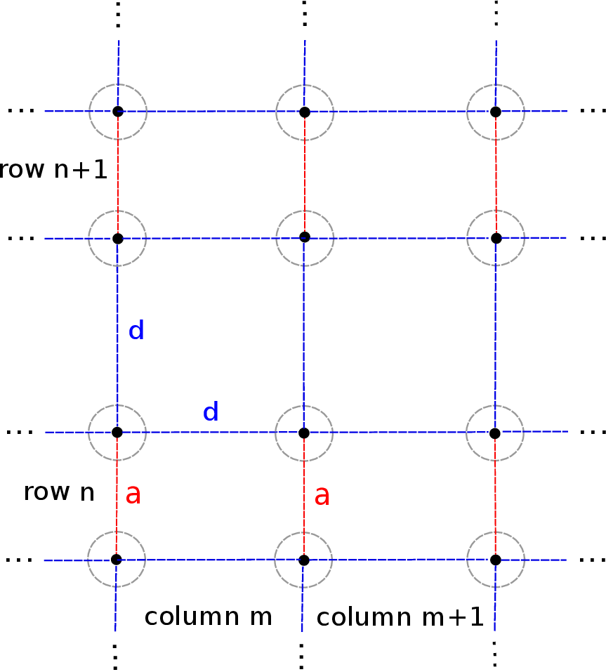
In the array geometry of Fig. 10, it should in principle be possible to entangle all qubits in a single row into an cluster state with one single detuning pulse (similarly as in Fig. 9). The neighboring rows can then be entangled with each other again sequentially in one step per a pair of rows. Entangling the rows with each other should not affect the entanglement inside rows as the detuning values required for large $E_{cc}$-values in the linear and parallel alignments differ considerably (see Fig. 4). The total number of entangling steps for obtaining a cluster state spanning the whole array is thus $M+1$. A cluster state corresponding to a given graph in the array can then be created by measuring the qubits that do not belong to the graph in the $\sigma_{z}$-basis, which effectively removes them from the cluster [15].

In reality, however, fabricating perfectly symmetrical qubit arrays is impossible. The asymmetries in the array probably inhibit the one-step preparation of cluster states for entire rows of qubits. Instead, the preparation has to be done one qubit-pair at a time, or at least between row and column segments instead of whole rows and columns. There are also many other experimental limitations, including how the electrostatic gating defining the quantum dot potentials should be conducted in such arrays. The experimental issues are however outside the scope of this paper and the analysis in this section should be considered a preliminary study on many-qubit arrays and cluster states in the $S-T_{0}$ qubit architecture.

References

- [1] D. Loss and D. P. DiVincenzo, Phys. Rev. A 57, 120 (1998).
- [2] J. Levy, Phys. Rev. Lett. 89, 147902 (2002).
- [3] J. Taylor, H. Engel, W. Dür, A. Yacoby, C. Marcus, P. Zoller, and M. Lukin, Nat. Phys. 1, 177 (2005).
- [4] J. Petta, A. Johnson, J. Taylor, E. Laird, A. Yacoby, M. Lukin, C. Marcus, M. Hanson, and A. Gossard, Science 309, 2180 (2005).
- [5] S. Foletti, H. Bluhm, D. Mahalu, V. Umansky, and A. Yacoby, Nat. Phys. 5, 903 (2009).
- [6] M. Shulman, O. Dial, S. Harvey, H. Bluhm, V. Umansky, and A. Yacoby, Science 336, 202 (2012).
- [7] D. Stepanenko and G. Burkard, Phys. Rev. B 75, 085324 (2007).
- [8] R. Horodecki, P. Horodecki, M. Horodecki, and K. Horodecki, Rev. Mod. Phys. 81, 865 (2009).
- [9] D. M. Greenberger, M. A. Horne, A. Shimony, and A. Zeilinger, American Journal of Physics 58, 1131 (1990).
- [10] W. Dür, G. Vidal, and J. I. Cirac, Phys. Rev. A 62, 062314 (2000).
- [11] V. Coffman, J. Kundu, and W. K. Wootters, Phys. Rev. A 61, 052306 (2000).
- [12] H. J. Briegel and R. Raussendorf, Phys. Rev. Lett. 86, 910 (2001).
- [13] M. Borhani and D. Loss, Phys. Rev. A 71, 034308 (2005).
- [14] R. Raussendorf and H. J. Briegel, Phys. Rev. Lett. 86, 5188 (2001).
- [15] R. Raussendorf, D. E. Browne, and H. J. Briegel, Phys. Rev. A 68, 022312 (2003).
- [16] A. Barenco, C. H. Bennett, R. Cleve, D. P. DiVincenzo, N. Margolus, P. Shor, T. Sleator, J. A. Smolin, and H. Weinfurter, Phys. Rev. A 52, 3457 (1995).
- [17] A. Johnson, J. Petta, J. Taylor, A. Yacoby, M. Lukin, C. Marcus, M. Hanson, and A. Gossard, NATURE 435, 925 (2005).
- [18] F. H. L. Koppens, J. A. Folk, J. M. Elzerman, R. Hanson, L. H. W. van Beveren, I. T. Vink, H. P. Tranitz, W. Wegscheider, L. P. Kouwenhoven, and L. M. K. Vandersypen, Science 309, 1346 (2005).
- [19] A. V. Khaetskii, D. Loss, and L. Glazman, Phys. Rev. Lett. 88, 186802 (2002).
- [20] I. A. Merkulov, A. L. Efros, and M. Rosen, Phys. Rev. B 65, 205309 (2002).
- [21] X. Hu and S. Das Sarma, Phys. Rev. Lett. 96, 100501 (2006).
- [22] O. E. Dial, M. D. Shulman, S. P. Harvey, H. Bluhm, V. Umansky, and A. Yacoby, Phys. Rev. Lett. 110, 146804 (2013a).
- [23] I. van Weperen, B. D. Armstrong, E. A. Laird, J. Medford, C. M. Marcus, M. P. Hanson, and A. C. Gossard, Phys. Rev. Lett. 107, 030506 (2011).
- [24] G. Ramon and X. Hu, Phys. Rev. B 81, 045304 (2010).
- [25] G. Ramon, Phys. Rev. B 84, 155329 (2011).
- [26] E. Nielsen, R. W. Young, R. P. Muller, and M. S. Carroll, Phys. Rev. B 82, 075319 (2010).
- [27] T. Hiltunen, J. Ritala, T. Siro, and A. Harju, New Journal of Physics 15, 103015 (2013).
- [28] J. Nickolls, I. Buck, M. Garland, and K. Skadron, Queue 6, 40 (2008).
- [29] O. E. Dial, M. D. Shulman, S. P. Harvey, H. Bluhm, V. Umansky, and A. Yacoby, Phys. Rev. Lett. 110, 146804 (2013b).
- [30] J. Särkkä and A. Harju, New J. Phys. 13, 043010 (2011).
- [31] E. Nielsen, R. P. Muller, and M. S. Carroll, Phys. Rev. B 85, 035319 (2012).
- [32] T. Hiltunen and A. Harju, Phys. Rev. B 89, 115322 (2014).