Discrimination on the Grassmann Manifold: Fundamental Limits of Subspace ClassifiersThanks: This work supported in part by AFOSR grant FA9550-13-1-0076 and the Royal Society International Exchanges Scheme IE120996. Preliminary elements of this work were presented at the IEEE Information Theory Workshop, Sept. 2013 and the IEEE Symposium on Information Theory, July 2014. Matthew Nokleby and Robert Calderbank are with Duke University, Durham, NC (emails: {matthew.nokleby,robert.calderbank}@duke.edu), and Miguel Rodrigues is with University College London (email: m.rodrigues@ucl.ac.uk)
Abstract
We present fundamental limits on the reliable classification of linear and affine subspaces from noisy, linear features. Drawing an analogy between discrimination among subspaces and communication over vector wireless channels, we propose two Shannon-inspired measures to characterize asymptotic classifier performance. First, we define the classification capacity, which characterizes necessary and sufficient conditions for the misclassification probability to vanish as the signal dimension, the number of features, and the number of subspaces to be discerned all approach infinity. Second, we define the diversity-discrimination tradeoff which, by analogy with the diversity-multiplexing tradeoff of fading vector channels, characterizes relationships between the number of discernible subspaces and the misclassification probability as the noise power approaches zero. We derive upper and lower bounds on these measures which are tight in many regimes. Numerical results, including a face recognition application, validate the results in practice.
I Introduction
The classification of high-dimensional signals arises in a host of situations, from face and digit recognition [1, 2, 3] to tumor classification [4, 5], and to the music-identification app Shazam [6]. These problems involve massive data sets—images with millions of pixels, DNA arrays with thousands of genes, or audio clips with tens of thousands of samples—which presents a substantial burden of computation and storage. Frequently, however, the data lie near a low-dimensional subspace of ambient space. For example, images of an individual’s face, subject to constraints on pose, lighting, and convexity, lie almost entirely on a subspace of five to nine dimensions, regardless of the ambient dimension of the image [7, 8, 9]. One therefore can pose classification tasks like face recognition as subspace classification problems.
When identifying low-dimensional subspaces, one can reduce the computation and storage burden by classifying from a low-dimensional representation of the signal of interest. This process is called feature extraction, and standard techniques, including linear discriminant analysis (LDA) and principal component analysis (PCA) [10], as well as their myriad variations, are well studied. One pays a price, however, for computational tractability. In principle, extracting low-dimensional features from high-dimensional signals degrades classifier performance, and it is unclear a priori how many features are necessary to ensure success.
In this paper, we present a rigorous, information-theoretic characterization of classifier performance of high-dimensional data from low-dimensional features. We show that performance depends on several factors, including the number of subspaces to be discriminated, the number of features extracted, and the underlying subspace structure. In particular, we consider the classification of -dimensional linear and affine subspaces of from linear features corrupted by Gaussian noise. To characterize classifier performance, we define two performance measures:
- •
The classification capacity, which characterizes the number of unique subspaces that can be discerned as a function of the noise power, , , and , as the latter three quantities approach infinity. Just as the usual Shannon capacity captures the phase transition of the error probability, as a function of the information rate, as the code length goes to infinity, the classification capacity captures the phase transition of the misclassification probability, in terms of the (logarithm of the) number of subspaces, as the signal dimension goes to infinity.
- •
The diversity-discrimination tradeoff (DDT), which characterizes the relationship between the number of subspaces and the misclassification probability as the noise power goes to zero. Just as the diversity-multiplexing tradeoff for fading vector wireless channels [11] characterizes the number of codewords and the error probability in terms of a region of achievable exponent pairs in the signal-to-noise ratio (SNR), the DDT specifies a region of achievable exponent pairs in the noise power for the number of subspaces and the misclassification probability.
The motivation for the preceding definitions is an analogy between classification from noisy features and communication over non-coherent vector channels. Indeed, the title of our paper alludes to [12], which investigates the capacity of the block-fading non-coherent channel in geometric terms. It shows that, at high SNR and for sufficiently long coherence time, transmitters achieve near-capacity rates by sending subspaces as codewords. Therefore the decoding task is to discern subspaces from noisy observations, and the capacity corresponds to asymptotic packings in the Grassmann manifold. Further works give tighter bounds on the capacity and explore the diversity-multiplexing tradeoff of the non-coherent channel [12, 13, 14, 15].
For the classification of -dimensional linear subspaces from noisy, linear features, one can demonstrate a syntactic duality with communications over non-coherent vector channels. Specifically, the classification problem is dual to a non-coherent communications over a channel with transmit antennas, a single receive antenna, and a coherence time of . In a preliminary version of this work, we applied results from [12, 14] directly to prove necessary conditions for successful classification [16].Ê These bounds translate into upper bounds on the classification capacity and diversity-discrimination tradeoff considered in this paper.
However, these bounds are somewhat crude. In the dual communications problem, the optimal transmission strategy employs only a single transmit antenna, which is equivalent to classifying subspaces of dimension . Therefore, the upper bounds are loose when classifying subspaces of higher dimension. Furthermore, because the classification problem is not known to be information stable [17], the mutual information between subspaces and features does not lower bound the classification capacity even for . To prove tighter upper bounds on performance, we develop new bounds on the mutual information, and to prove lower bounds on performance we analyze the misclassification probability directly.
I-A Summary of Results
Our primary contributions are upper and lower bounds, which are tight in many regimes, on the classification capacity and the diversity-discrimination tradeoff.
In Section III, we study the classification capacity. First we consider the classification of linear subspaces, which we model by taking the classes to follow zero-mean Gaussian distributions with approximately low-rank covariances. The covariances have two components: a rank component corresponding to the class subspace, and an identity component scaled by corresponding to deviations from the subspace. We further suppose a prior distribution the subspaces which is uniform over the Grassmann manifold of -dimensional subspaces in . We present an upper bound on the classification capacity, showing almost surely that the number of subspaces cannot scale any faster than . This result is intuitive: The lower the inherent signal dimension, the fewer features are required to classify the signal reliably. We also present a lower bound on the classification capacity, showing that the misclassification probability decays to zero, except for a set of subspaces having vanishing probability, provided the number of subspaces grows slower than . When , the bounds are tight up to a term. Furthermore, based on simulations presented in Section V, we conjecture that the upper bound is tight and that the gap between lower and upper bounds when is merely an artifact of the analysis.
We then consider the classification of affine subspaces, or linear subspaces translated by nonzero points. We model affine spaces by taking the classes to again be modeled by approximately rank- covariances, but this time to have nonzero means. We again suppose a uniform prior over the Grassmann manifold, and we further suppose that the means are distributed according to a standard Gaussian distribution. We characterize the classification capacity up to a term, showing that the number of subspaces growing no faster than is both necessary and sufficient for the probability of error to decay to zero, again except for a set of subspaces having vanishing probability.
In Section IV, we study the diversity-discrimination tradeoff. For linear subspaces, we derive an upper bound, showing that the average misclassification probability decays no faster than as and that the misclassification probability exhibits an error floor when the number of subspaces scales faster than . We also derive a lower bound, showing that the misclassification capacity decays at least as when the number of subspaces scales as . For affine spaces, we specify the DDT exactly, showing that the average probability decays as when the number of subspaces scales as .
For both linear and affine subspace classification, the lower bounds on performance are realized by any feature matrix having orthonormal rows in . Therefore, for regimes in which the bounds are tight, the asymptotic performance as characterized by the classification capacity and DDT is invariant to rotations of the linear features.
In Section V, we evaluate our claims empirically. We first examine the error performance of classifiers over randomly-drawn linear subspaces, focusing on the regimes in which the upper and lower bounds disagree. Then, we test the correspondence of our theoretical results to a practical face recognition application. Using standard classification algorithms against public datasets, we observe error performance that agrees with our predictions to within a reasonable tolerance.
I-B Prior Work
The statistics and machine learning literature contains a large body of work on feature extraction or supervised dimensionality reduction. In addition to the venerable linear discriminant analysis and principal component analysis, which depend only on the second-order statistics of the data, linear techniques based on higher-order statistics were developed in[18, 19, 20, 21, 22, 23, 24, 25, 26]. Owing to Fano’s inequality, the algorithm of [18] chooses linear features having maximal the mutual information with the classes, whereas [20, 25, 26] employ approximations to the mutual information based on Rényi entropy. In [27] linear features are chosen for subspace classification according to a nuclear-norm optimization problem, and in [28] an LDA-inspired Grassmann discriminant analysis is proposed. Finally, nonlinear dimensionality reduction techniques have recently become popular [29, 30].
In the signal processing literature, information-theoretic limits on subspace classification arise under the framework of sparse support recovery. The set of all -sparse vectors in is a union of subspaces, and recovering the sparsity pattern is equivalent to finding the subspace in which the signal lies. A (data) deluge of recent works [31, 32, 33, 34, 35, 36, 37, 38, 39, 40, 41, 42, 43] provides necessary and sufficient scaling laws on the triplet , where is the number of compressive measurements taken, for recovery of a sparse signal. Different assumptions on the measurement matrices, decoders, error metrics, and sparsity regimes give rise to different scaling laws. While these works do provide fundamental limits on subspace classifier performance, sparse support recovery entails a specialization to the union of canonical subspaces, and the results presented in the preceding works do not bear directly on our study.
Reference [44] considers compressed learning, i.e. learning directly in the compressive measurement domain rather than in the original data domain, showing that when data admit a sparse representation, low-dimensional feature extraction preserves the learnability and the separability of the data. Along a similar vein, a recent work [45] considers the compressive classification of convex sets, proving limits on the number of measurements required to ensure that the projected sets remain separated.
A few works have focused on the classification of Gaussian mixtures, which is closely related to the linear and affine subspace classification considered herein. In [46] classifier performance is studied for a finite number of classes as a function of signal geometry; these results prefigure the DDT results presented in the sequel. In [47], the number of measurements required to classify and reconstruct a signal drawn from a Gaussian mixture is characterized.
Researchers have also studied information-theoretic limits on other classification problems. The authors of [48] provide asymptotic limits on the success of model selection of Markov random fields. The authors of [49] use results in universal source coding to prove general bounds on classifier performance. The authors of [50] study the limits of database recovery from low-dimensional features, characterizing an “identification capacity” which is analogous to the classification capacity studied in this paper.
I-C Notation
We let bold lowercase letters denote vectors and bold uppercase letters to denote matrices. We let and denote the field of reals and integers, respectively. We let and denote the identity matrix and the all-zeros matrix, respectively, indicating the size of the matrix in a subscript when necessary. We let denote the Euclidean norm; when applied to a matrix it denotes the induced operator norm. We let denote the expectation, indicating the distribution over which the expectation is taken by a subscript when necessary. We let and denote the floor function and the positive part of a number, respectively. We let denote the vector of eigenvalues of a square matrix. We let denote equality in distribution. We let denote a Gaussian distribution with mean and covariance matrix . We let denote the Wishart distribution with degrees of freedom and shape matrix .
II Preliminaries
II-A Problem Definition
We consider the statistical classification problem, in which the signal of interest is distributed according to one of class-conditional densities , each of which is known to the classifier. The classifier observes noisy linear projections of , from which it attempts to determine the class-conditional density from which was drawn. These projections, denoted by , are related to the signal as follows:
| (1) |
where is a matrix describing the linear features, and is white Gaussian noise with mean zero and per-component variance for some . We suppose , and we constrain . The noise describes the deviation between the postulated subspace model and the true signal of interest.11 1 Equivalently, we could remove the additive noise and add a term to the covariance matrix of each class-conditional density. Signals will not lie perfectly on the linear or affine subspaces, so we suppose that the projected signal lies approximately within a ball centered at the specified subspaces and having radius .
To model the classification of linear and affine subspaces, we impose structure on the class-conditional densities . In particular, we suppose that the class conditional densities are Gaussian with low-rank covariances that correspond to the subspaces. In the case of linear subspaces, these Gaussians have zero mean. In the case of affine subspaces, which are simply translations of linear subspaces, the Gaussians have nonzero means.
We therefore define two sets. For the classification of -dimensional linear subspaces of , the class-conditional densities belong to22 2 We will drop the subscripts and throughout when discussing classification generally rather than particularizing to linear or affine subspaces.
| (2) |
In other words, each class-conditional density is a Gaussian supported on the -dimensional subspace spanned by the columns of . Similarly, for the classification of -dimensional affine spaces, the class-conditional densities belong to
| (3) |
That is, the class-conditional densities are supported on a -dimensional subspace as before, but here they are translated by a non-zero vector .
We parameterize the sets and by the following two sets
| (4) | ||||
| (5) |
Clearly and are isomorphic to and , respectively. We can represent a linear or affine subspace classification problem by a tuple , where is the -fold Cartesian product of . The tuple encodes the covariances and, when appropriate, the means corresponding to the subspaces to be classified. Let , for , denote the class-conditional densities parameterized by .
Let denote the classifier output, where is a mapping from to . Then, for a classification problem described by the tuple , define the average misclassification probability:
| (6) |
where each term in the sum is the misclassification probability when is drawn according to . Observe that we define in terms of the best feature matrix . Therefore, in proving our results we will characterize the feature matrix that achieves optimal classifier performance in the asymptote.
The focus of this paper is the analysis of in two asymptotic regimes: (i) as the signal dimensions go to infinity, and (ii) as the noise power goes to zero. In the first case, we derive conditions for which the probability of error decays to zero, except for a set of vanishing probability over . In the second case, we derive scaling laws on the probability of error, averaged over the possible choices of . To this end, define the following probability distributions over the parameter sets and :
| (7) | ||||
| (8) |
where is the th element of the matrix and is the th element of the vector . These distributions define a measure over the sets of class-conditional densities. In other words, in computing probabilities we suppose that the elements of the matrix and the mean vector are standard i.i.d. Gaussian.
For both and , the distribution is supported over the entire parameter space, is invariant to rotations, and yields finite expected signal energy. Specifically, the distribution over the bases is isotropic, which means that the linear subspaces are drawn uniformly from the Grassmann manifold. Therefore, our analysis characterizes classifier performance when “nature” presents us with subspaces without favoring a particular region of the Grassmann; we contend that this assumption is reasonable. Furthermore, while changes to the distributions and will change the classification capacity and DDT in general, the coarse behavior is robust to variations. In particular, one can recover our proofs subject to straightforward constraints on the eigenvalue distribution of , showing bounds on the classification capacity that differ at most by a term and DDT bounds that agree exactly.
Next, we define the classification capacity and the diversity-discrimination tradeoff.
II-B Classification Capacity
The classification capacity characterizes fundamental performance limits as the signal dimensions approach infinity. We derive bounds on how fast the number of subspaces can grow, as a function of , , and , while ensuring the misclassification probability decays to zero almost surely.
By analogy with the sequence of codebooks defined for the Shannon capacity, we characterize the classification capacity in terms of a sequence of classification problems indexed by . We let the number of features grow to infinity, and we let the dimensions and scale linearly with as follows:
| (9) |
for and . We also let the number of subspaces scale exponentially in as follows:
| (10) |
for some . By analogy with communications theory, the quantity can be interpreted as the “rate” of the sequence of class alphabets, or the average number of bits discerned per feature if classification succeeds. Indeed, in the sequel we refer to a the classification rate.
Definition 1
Fix the dimension ratios and and the classification rate . Then, define the set of classification problems for which the probability of classification error exceeds an arbitrary small constant :
| (11) |
Then, we say that is achievable provided
| (12) |
for any fixed .
Observe that a classification rate is achievable if
| (13) |
This observation follows by contradiction: If there is a subset of having non-trivial probability for which the misclassification probability remains bounded away from zero, the expected error also remains bounded away from zero.
Definition 2
Fix the dimension ratios and . The classification capacity, denoted by and for linear and affine space classification, respectively, is the supremum over achievable classification rates .
In other words, if the classification rate is smaller than , then the probability of classification error approaches zero almost surely over the set of subspace classification problems. Otherwise, the error probability remains bounded away from zero for a non-trivial subset of .
Although the classification capacity is defined to characterize classifier behavior when and scale linearly in and scales exponentially in , it also captures other regimes automatically. For example, if scales sub-linearly in , the asymptotic behavior is the same as if . Similarly, if scales sub-exponentially in , the misclassification probability decays to zero whenever the classification capacity is nonzero, and if scales super-exponentially the misclassification capacity remains bounded from zero whenever the classification capacity is finite. In view of Theorems 1 and 2, this implies that whenever and the number of subspaces grows polynomially in , the misclassification probability goes to zero. Because we are dealing with subspaces, it is impossible to have scale sub-linearly or scale super-linearly in . However, at least one regime remains unspecified by our analysis: If scales super-linearly in , classifier behavior is unclear.
We can bound the classification capacity via the mutual information between the vector and the feature vector .
Lemma 1
The classification capacity satisfies
| (14) |
where the mutual information is computed with respect to or as appropriate.
Proof:
The proof follows from Fano’s inequality. By the standard arguments (e.g. from [51]), we obtain
which is bounded away from zero when exceeds the RHS of (14). ∎
Observe that we have proven more than just an upper bound on the capacity. When exceeds RHS of (14), not only is there a non-trivial set for which the error probability remains positive, but that set is also all of . If the upper bound of Lemma 1 is tight, then the mutual information characterizes a sharp phase transition in the error probability. If the number of subspaces grows sufficiently slowly, the probability of error vanishes almost everywhere; otherwise, is bounded away from zero everywhere.
However, it is not clear whether Lemma 1 is tight. If the “channel” between subspaces and features is information stable—meaning roughly that the normalized information density converges on the normalized mutual information—then the mutual information completely characterizes the classification capacity and (14) holds with equality [17]. Alternatively, applying the results of [52], one can express the classification capacity directly in terms of the information density. Analysis of the information density is difficult, however, as is the verification of information stability, so Lemma 1 remains an upper bound only.
To prove lower bounds on the classification capacity, we analyze directly the misclassification probability. Our main tool is the Bhattacharyya bound on the pairwise misclassification probability[53, 54], which we state here for Gaussian distributions.
Lemma 2
Suppose we observe a signal that is distributed according to or with equal prior probability. Define
| (15) |
Then, supposing maximum likelihood classification, the misclassification probability is bounded by
| (16) |
In [54] it is also observed that the Bhattacharyya bound is exponentially tight in the sense that, if the pairwise error decays to zero, it approaches for some constant . A consequence of this observation, which we will see in Section IV, is that the Bhattacharyya bound predicts the maximum diversity gain for both linear and affine subspace classifiers.
II-C Diversity-Discrimination Tradeoff
The diversity-multiplexing tradeoff (DMT) was introduced in the context of wireless communications to characterize the high-SNR performance of fading vector channels. It was shown in [11] that the spatial flexibility provided by multiple antennas can simultaneously increase the achievable rate and decrease the probability of error, but only according to a tradeoff that is precisely characterized at high SNR. We define a similar characterization in the context of classification, called the diversity-discrimination tradeoff (DDT), which captures the relationship between the increase of discernible subspaces and the decay of misclassification probability as the noise power approaches zero.
For the DDT, we keep , , and fixed, but we let the number of subspaces scale in the noise power as follows:
| (17) |
for some , which we call the discrimination gain. We define the DDT in terms of the misclassification probability averaged over the ensemble of classification problems, which we denote by
| (18) |
where here we express the probability of error as a function of the discrimination gain and the noise power . Specifically, the diversity-discrimination tradeoff is defined as the following function:
| (19) |
We refer to as the diversity gain for discrimination gain . In other words, when the number of subspaces increases as , the probability of error decays as . In the sequel we refer to and as appropriate.
By contrast to the classification capacity, where we characterize phase transitions in the error probability that hold almost surely, for the DDT we specify scaling laws in the error probability that hold on the average over . Rather than specifying if the probability of error decays to zero, the DDT specifies how quickly it decays. In the former case, it is straightforward to define the failure event and show that it has vanishing probability. In the latter case, it is unclear how to define such a failure event, so we state only an average-case result.
As with the classification capacity, we can derive bounds on the DDT from the mutual information.
Lemma 3
Fix , , and . Then, whenever
| (20) |
where again the mutual information is calculated with respect to or as appropriate.
Proof:
Again we invoke Fano’s inequality. Whenever is as large as the specified quantity, the probability of error is bounded away from zero, and the diversity gain is zero by definition. ∎
III Classification Capacity
Here we characterize the classification capacities and . We prove upper bounds that show that, for both linear and affine subspace classification, the probability of error remains bounded away from zero almost surely whenever the number of subspaces scales faster than . For linear spaces, we prove a lower bound which matches the upper bound to within an term for ; otherwise the bounds disagree. For affine spaces, we prove a lower bound which is tight to within an term for all . This suggests the somewhat surprising conclusion that, at least for , translating subspaces by nonzero vectors does not substantially increase the number of subspaces a classifier can discriminate. Whether this conclusion extends to depends on the tightness of the upper bound. However, as we will see in Section IV, affine subspaces are easier to discriminate in the sense that the misclassification probability decays faster as .
III-A Linear Subspaces
First, we bound on .
Theorem 1
For linear subspace classification, the classification capacity is bounded by
| (21) |
Proof:
We first prove the upper bound by estimating the mutual information between the subspaces and the features and invoking Lemma 1. Then, we prove the lower bound by invoking Lemma 2 and applying the union bound.
Upper Bound: To bound the mutual information , we first characterize the optimum choice of . Following the argument in [18, Theorem 2], we compute the gradient of the mutual information with respect to the singular values of . Writing the singular value decomposition as , the gradient is
| (22) |
where
is the mean with respect to the posterior distribution, and
is the mean with respect to the conditional posterior. Observe from (22) that the diagonal elements of the gradient are non-negative, which implies that the mutual information is non-decreasing with the singular values of . Because we constrain , it follows that the singular values of the optimal are identically unity.
Assuming this condition on , we bound the mutual information. By definition,
To bound the conditional entropy, observe that the conditional distribution of is
Let denote the th ordered eigenvalue of . Then, the conditional entropy is
where the expectation is with respect to , and where the inequality is trivially obtained by substituting the smallest positive eigenvalue . We next bound this eigenvalue. Because has singular values identically equal to unity, and because has i.i.d. Gaussian entries with variance , the matrix also has i.i.d. Gaussian entries with variance . Therefore,
where . In [55, Theorem 1] it is shown that the smallest eigenvalue of converges to almost surely as . Therefore, the minimum eigenvalue of , which is equal to , converges on almost surely. We can therefore bound the conditional mutual information by
| (23) |
where as .
We turn next to the differential entropy of . We first compute the expected covariance, which is
Noting that the differential entropy for a fixed covariance is maximized by the multivariate Gaussian distribution, we obtain
| (24) |
Combining terms and letting , we finally obtain
| (25) |
Lower Bound: Choose to be any matrix with orthonormal rows. Observe that while this choice maximizes the mutual information, it does not minimize the probability of error in general. Applying the Bhattacharyya bound from Lemma 2, the probability of a pairwise error between two subspaces and is bounded by
With probability one, the matrices and have rank , and the matrix has rank . Let and denote the nonzero eigenvalues of and , respectively, and let denote the nonzero eigenvalues of the latter matrix. Then, we can write the pairwise bound as
By construction,
By Weyl’s monotonicity theorem (see, e.g., [56]), and for every . Therefore,
from which it follows that
Next, we bound the eigenvalue . Because each matrix has i.i.d. Gaussian entries with zero mean and variance , so too does each matrix . Furthermore, observe that
Therefore, the nonzero eigenvalues of are those of a scaled Wishart matrix. Specifically, if , the eigenvalues are those of , where . If , the eigenvalues are those of , where . By [55, Theorem 1], the minimum eigenvalue in either case converges on almost surely. Therefore, converges on almost surely, and we obtain
| (26) |
where almost surely as . A fortiori, the bound in (26) is also a bound on the expected pairwise probability, with independent for each pair.
Invoking the union bound over all subspaces, we obtain
where the second equality follows because each is drawn independently. Taking the logarithm of both sides yields
| (27) |
Therefore, if
then goes to zero as , and thus goes to zero almost surely, as was to be shown. ∎
When , the lower and upper bounds agree to within a term; otherwise they are loose. Based on the numerical experiments presented in Section V, we conjecture that the upper bound is approximately tight, while the lower bound is loose.
III-B Affine Subspaces
Next, we bound .
Theorem 2
For affine subspace classification, the classification capacity satisfies
| (28) |
and
| (29) |
Proof:
As before, we prove the upper bound by bounding the mutual information, and the lower bound by direct analysis of the probability of error via the Bhattacharyya bound.
Upper Bound: To prove the upper bound, we expand the mutual information as
| (30) |
As in the case of linear subspaces, the that maximizes the mutual information has unit singular values. Furthermore, because the entropy of a Gaussian does not depend on the mean, . Therefore, applying (23), we obtain
| (31) |
where . Then, observing that
we conclude that
| (32) |
from which it follows that
| (33) |
Applying the preceding to Lemma 1, we obtain the upper bound.
Lower Bound: Suppose that we choose to be any matrix with orthonormal rows. We bound the pairwise misclassification error via Lemma 2, which yields
| (34) |
Observe that the argument of the exponential term is always nonnegative, so the exponential is always smaller than one. Therefore, the bound on the misclassification probability of affine subspaces is always smaller than that of linear subspaces, and the lower bound from Theorem 1 also applies to affine subspaces. Applying this fact yields the lower bound for .
For , we apply (26) to (34), yielding
| (35) |
where again . Next, let be the eigenvalue decomposition of the covariance pair sum. Also define , which is i.i.d. Gaussian with zero mean and unit variance. We therefore obtain
With probability one, contains nonzero eigenvalues. The preceding bound increases in these eigenvalues, so to bound the error we bound the eigenvalues by infinity, which yields
Taking the expectation yields
where the expectation moves inside the product because each is independent of the others. Noting that each expectation in the final expression is just the moment-generating function of a Chi-squared random variable, we obtain
| (36) |
Applying the union bound and taking the logarithm, we obtain
| (37) | ||||
| (38) |
Letting , we obtain the lower bound for . ∎
For affine subspaces, the bounds are tight to within an term for all values of . Roughly speaking, the term in the Bhattacharyya bound associated with discriminating the means cancels out the gap to the upper bound associated with discriminating the associated linear subspaces. Therefore pairwise analysis, along with the union bound, is sufficient for establishing tight bounds on the classification capacity for affine subspaces even when it fails for linear subspaces.
IV Diversity-discrimination Tradeoff
Here we prove bounds on the diversity-discrimination tradeoff. Similar to the classification capacity, we prove an upper bound on , which shows that the maximum diversity gain is and the maximum discrimination gain is . We also prove a lower bound, based on the Bhattacharyya bound, which establishes that the average misclassification probability decays at least as when the number of subspaces grows as . For affine subspaces, we prove an upper bound which shows that the misclassification probability decays no faster than . In this case, the Bhattacharyya analysis shows that the upper bound is tight.
IV-A Linear Subspaces
First, we prove bounds on .
Theorem 3
For linear subspaces, the DDT is upper bounded by
| (39) |
and the DDT is bounded below by
| (40) |
Proof:
First we prove the upper bound, the first term of which follows from Lemma 3. Combining (23) and (24), it is easy to see that
| (41) |
Therefore, by Lemma 3, whenever . Next, suppose that for some , meaning that, for some ,
| (42) |
Using the union bound, we can express the probability of error for in terms of (42):
This implies , which is a contradiction.
The second term in the upper bound follows from an “outage”-style argument reminiscent of that of [14]. For linear subspaces, we can rewrite the signal model (1) as
where . We define an outage event
| (43) |
for . Because each is Chi squared with a single degree of freedom,
| (44) |
Next, we bound the conditional normalized mutual information:
where the inequality follows because (i) the Gaussian distribution maximizes mutual information, and (ii) by the entropy power inequality. Conditioned on the outage event, we have , from which it follows that
By the law of total probability,
By Lemma 3, whenever , the conditional probability is bounded away from zero. Therefore,
Taking , we obtain the second term of the upper bound.
The lower bound follows from the Bhattachayya analysis from Section III-A. For discrimination gain , we combine (26) with the union bound, yielding
Therefore, we have
∎
Similar to the classification capacity, the lower bound is tight when . Otherwise, the lower bound achieves full diversity for , but falls short of the upper bound for higher discrimination gain. Note, however, that the second term in (39), which establishes that the diversity gain is no greater than , is clearly loose because it predicts nonzero diversity for discrimination gains higher than . This looseness is due to the bound on the normalized mutual information, in which we employed ; this bound neglects the effect of the outage event on the eigenvalues.
A tighter bound on the conditional entropy is difficult because is no longer Gaussian conditioned on . However, we can make heuristic calculations by bounding the conditional covariance and supposing that the entropy is approximately that of the equivalent Gaussian. Then, the normalized mutual information is instead bounded by . Following that analysis leads to the following bound on DDT function
| (45) |
This function is just the line segment connecting the maximum diversity order and the maximum discrimination gain in the upper bound. Based on the preceding intuition and the numerical results in Section V, we conjecture that this is the true diversity-discrimination tradeoff for linear classification.
IV-B Affine Subspaces
Next, we derive .
Theorem 4
For affine subspace classification, the DDT is
| (46) |
Proof:
We can upper bound the DDT using the same argument as in the proof of Theorem 3. Combining (31) and (32), we obtain
| (47) |
Therefore, for by Lemma 3. As before, by the union bound there is a contradiction if for any .
To lower bound the DDT, observe from the proof of Theorem 2 that
| (48) |
For discrimination gain , the union bound yields
| (49) |
which establishes the result. ∎
For affine spaces, similar to the classification capacity, the upper bound is tight. Therefore, the Bhattacharyya bound is tight not only with respect to the pairwise error, but also upon application of the union bound. Therefore, while the translation of linear subspaces into affine subspaces does not necessarily improve the number of subspaces that a classifier can discriminate reliably, for translation does improve the decay of the error probability as the noise power vanishes.
V Numerical Results
Here we validate our results numerically. First, we study the performance of linear subspace classifiers with subspaces drawn randomly from , focusing on the regimes in which the upper and lower bounds disagree and drawing conclusions about the tightness of the bounds. Then, we study the classifier performance over the YaleB database of face images, comparing empirical performance to the predictions of Section III.
V-A Linear Subspaces
Here, we want to see whether the upper bound on the is tight for , as we conjectured in Section III-A. We also want to see whether the diversity-discrimination function we conjectured in Section IV-A is correct.
To answer these questions, we examine classifier performance as . We draw subspaces from and we choose to be the first rows of a randomly-chosen unitary matrix. We corrupt the features with white Gaussian noise of variance , and we perform maximum-likelihood classification on the noisy features. Because of computational limitations, it is infeasible to study empirical performance as the signal dimension becomes large. Therefore, instead of testing the classification capacity directly, we examine the DDT performance. If, for discrimination gain , the diversity gain is nonzero, then the classification capacity must be at least as great as .
In Figure 1 we plot the misclassification probability as a function of . For each value of , we compute the average misclassification probability over realizations of the subspaces and realizations of the signal of interest per set of subspaces. We also plot the error slopes predicted by (45). We select dimensions , and discrimination gains . We observe decaying misclassification probability for all values of ; furthermore, we observe rates of decay consistent with the conjectured DDT function. Therefore, we conclude that, regardless of , the classification capacity satisfies
and that the DDT is
Recall that these conclusions were proven only in the regimes or .
V-B Face Recognition
Next, we explore the correspondence between the theoretical results derived in the previous sections and a practical face recognition application. We examine face recognition when the orientation of the face relative to the camera remains fixed but the illumination varies. Supposing the faces to be approximately convex and to reflect light according to Lambert’s law, [57] shows via spherical harmonics that the set of images of an individual face lies approximately on a nine-dimensional subspace, regardless of the inherent dimension of the images. It is therefore sufficient to discriminate between the subspaces to classify faces.
We use 38 cropped faces from the Extended Yale Face Database B, described in [7, 8]. For each face, the database contains a few dozen greyscale photographs, each having 32,256 pixels, taken under a variety of illumination conditions as shown in Figure 2. We vectorize these images and pass them through a feature matrix , chosen as before to be the first rows of an arbitrary unitary matrix. We classify the faces using the maximum-likelihood classifier supposing zero-mean Gaussian classes. We divide the database into two, using half of the images to estimate the nearest covariance for each face, using the other half as test images.


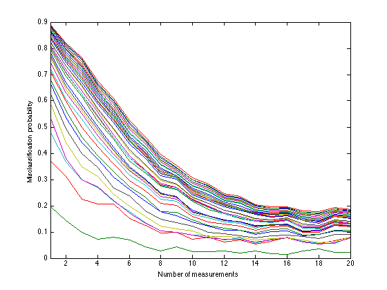
In Figure 3 we plot the misclassification probability as a function of and for ranging from 2 to 38. While we do not label each curve, it is easy to see that the misclassification probability increases with and decreases with . However, even for large the error probability remains as high as 0.2 for . We take 0.2 as a baseline for “successful” performance when the number of faces and signal dimension are high.
Finally, we examine how well our theory predicts the performance seen here. To estimate the noise power , we project each image onto its estimated subspace, transformed by , and we take take the projected squared norm as the signal power and the squared residual norm, normalized by the number of features , as the noise power. We then estimate the number of faces that Theorem 1 predicts can be discriminated reliably. Discarding the constants, we simply compute
| (50) |
Naturally, this number grows quickly in , and beyond or , theory suggests that we ought to be able to discriminate all 38 of the faces with low probability of error. In Figure 4 we compare this prediction against the empirical performance of our classifier. Using the results shown in Figure 3, we compute, for each , the maximum for which the probability of error is less than 0.2.
The empirical performance is similar to theoretical prediction. As increases past 9, the number of faces rises swiftly as predicted. After or so, all 38 of the faces can be discriminated, and it is not advantageous to extract more features. We do observe, however, that the transition is not as sharp as Theorem 1 predicts. Whereas the theoretical transition occurs over only 2-3 features, in practice the transition stretches out over 5-10 features. In addition to mild model mismatch due to non-Lambertian reflectances, shadows due to the non-convexity of real faces, imperfect estimation of subspaces, etc., we suspect that this is primarily a phenomenon of classification at finite dimension. The transition between success and failure becomes sharp in the limit, but remains gradual when dimensions measure in the tens or hundreds.
VI Conclusion
Inspired by dualities between wireless communication over non-coherent channels and the classification from noisy, linear features, we have derived fundamental limits on the classification of linear and affine subspaces from noisy, linear features. We defined performance limits reminiscent of those in wireless information theory: the classification capacity, which governs classifier performance in the limit of high signal dimension, and the diversity-discrimination tradeoff, which governs classifier performance in the limit of low noise power. We proved inner and outer bounds on these quantities. For linear subspaces, the bounds are tight in some regimes of , and , and for affine subspaces they are tight everywhere. Based on numerical evaluation, we conjectured that the true classification capacity and DDT for linear subspaces in the regimes in which the bounds are not tight. Beyond the characterization of such limits, we showed via an application to face recognition that theoretical trends agree reasonably with practical ones.
References
- [1] Y. Adini, Y. Moses, and S. Ullman, “Face recognition: The problem of compensating for changes in illumination direction,” Pattern Analysis and Machine Intelligence, IEEE Transactions on, vol. 19, no. 7, pp. 721–732, 1997.
- [2] J. J. Hull, “A database for handwritten text recognition research,” IEEE Trans. Pattern Analysis and Machine Intelligence, vol. 16, no. 5, pp. 550–554, 1994.
- [3] Y. LeCun, L. Jackel, L. Bottou, A. Brunot, C. Cortes, J. Denker, H. Drucker, I. Guyon, U. Muller, E. Sackinger et al., “Comparison of learning algorithms for handwritten digit recognition,” in International Conference on Artificial Neural Networks, vol. 60, 1995.
- [4] D. T. Ross, U. Scherf, M. B. Eisen, C. M. Perou, C. Rees, P. Spellman, V. Iyer, S. S. Jeffrey, M. Van de Rijn, M. Waltham et al., “Systematic variation in gene expression patterns in human cancer cell lines,” Nature Genetics, vol. 24, no. 3, pp. 227–235, 2000.
- [5] U. Alon, N. Barkai, D. A. Notterman, K. Gish, S. Ybarra, D. Mack, and A. J. Levine, “Broad patterns of gene expression revealed by clustering analysis of tumor and normal colon tissues probed by oligonucleotide arrays,” Proceedings of the National Academy of Sciences, vol. 96, no. 12, pp. 6745–6750, 1999.
- [6] [Online]. Available: http://www.shazam.com/
- [7] A. S. Georghiades, P. N. Belhumeur, and D. J. Kriegman, “From few to many: Illumination cone models for face recognition under variable lighting and pose,” IEEE trans. Pattern Analysis and Machine Intelligence, vol. 23, no. 6, pp. 643–660, 2001.
- [8] K.-C. Lee, J. Ho, and D. J. Kriegman, “Acquiring linear subspaces for face recognition under variable lighting,” IEEE Trans. Pattern Analysis and Machine Intelligence, vol. 27, no. 5, pp. 684–698, 2005.
- [9] R. Epstein, P. W. Hallinan, and A. L. Yuille, “52 eigenimages suffice: An empirical investigation of low-dimensional lighting models,” in Proc. the Workshop on Physics-Based Modeling in Computer Vision, 1995. IEEE, 1995.
- [10] R. A. Fisher, “The use of multiple measurements in taxonomic problems,” Annals of Eugenics, vol. 7, no. 2, pp. 179–188, 1936.
- [11] L. Zheng and D. Tse, “Diversity and multiplexing: a fundamental tradeoff in multiple-antenna channels,” IEEE Trans. Inform. Theory, vol. 49, no. 5, pp. 1073–1096, May 2003.
- [12] L. Zheng and D. N. C. Tse, “Communication on the Grassmann manifold: A geometric approach to the noncoherent multiple-antenna channel,” IEEE Trans. Info. Theory, vol. 48, no. 2, pp. 359–383, 2002.
- [13] T. L. Marzetta and B. M. Hochwald, “Capacity of a mobile multiple-antenna communication link in Rayleigh flat fading,” IEEE Trans. Info. Theory, vol. 45, no. 1, pp. 139–157, 1999.
- [14] L. Zheng and D. N. C. Tse, “The diversity-multiplexing tradeoff for non-coherent multiple antenna channels,” in Proc. Allerton, vol. 40, no. 2, 2002, pp. 834–843.
- [15] W. Yang, G. Durisi, and E. Riegler, “On the capacity of large-MIMO block-fading channels,” IEEE J. Select Areas Commun., vol. 31, no. 2, pp. 117–132, 2013.
- [16] M. Nokleby, M. Rodrigues, and R. Calderbank, “Information-theoretic limits on the classification of Gaussian mixtures: Classification on the Grassmann manifold,” in Proc. Information Theory Workshop (ITW), 2013.
- [17] R. Dobrushin, “General formulation of shannon’s main theorem in information theory,” Trans. American Mathematical Society, vol. 33, pp. 323–438, 1963.
- [18] M. Chen, W. Carson, M. R. D. Rodrigues, R. Calderbank, and L. Carin, “Communication inspired linear discriminant analysis,” in Proceedings of the 29th International Conference on Machine Learning, june 2012.
- [19] D. Erdogmus and J. C. Principe, “Lower and upper bounds for misclassification probability based on renyi’s information,” VLSI signal processing systems for signal, image and video technology, Journal of, vol. 37, no. 2 -3, pp. 305–317, 2004.
- [20] K. Hild, D. Erdogmus, K. Torkkola, and J. Principe, “Feature extraction using information-theoretic learning,” IEEE Trans. Pattern Analysis and Machine Intelligence, vol. 28, no. 9, pp. 1385–1392, 2006.
- [21] S. Kaski and J. Peltonen, “Informative discriminant analysis,” in Proceedings of the Twentieth International Conference on Machine Learning (ICML), 2003, pp. 329–336.
- [22] L. Liu and P. Fieguth, “Texture classification from random features,” Pattern Analysis and Machine Intelligence, IEEE Transactions on, vol. 34, no. 3, pp. 574 –586, march 2012.
- [23] Z. Nenadic, “Information discriminant analysis: Feature extraction with an information-theoretic objective,” Pattern Analysis and Machine Intelligence, IEEE Transactions on, vol. 29, no. 8, pp. 1394 –1407, august 2007.
- [24] D. Tao, X. Li, X. Wu, and S. Maybank, “Geometric mean for subspace selection,” Pattern Analysis and Machine Intelligence, IEEE Transactions on, vol. 31, no. 2, pp. 260–274, 2009.
- [25] K. Torkkola, “Learning discriminative feature transforms to low dimensions in low dimensions,” in Advances in neural information processing systems 14 (NIPS). MIT Press, 2001, pp. 3–8.
- [26] ——, “Feature extraction by non-parametric mutual information maximization,” Machine Learning Research, Journal of, vol. 3, pp. 1415–1438, March 2003.
- [27] Q. Qiu and G. Sapiro, “Learning robust subspace clustering,” CoRR, vol. abs/1308.0273, 2013.
- [28] J. Hamm and D. D. Lee, “Grassmann discriminant analysis: a unifying view on subspace-based learning,” in Proceedings of the 25th international conference on Machine learning. ACM, 2008, pp. 376–383.
- [29] J. Tenenbaum, V. de Silva, and J. Langford, “A global geometric framework for nonlinear dimensionality reduction,” Science, vol. 290, no. 5500, pp. 2319–2323, December 2000.
- [30] L. Wang, A. Razi, M. D. Rodrigues, and R. Calderbank, “Nonlinear information-theoretic compressive measurement design,” in Proc. International Conference on Machine Learning, 2014.
- [31] S. Aeron, V. Saligrama, and M. Zhao, “Information theoretic bounds for compressed sensing,” Information Theory, IEEE Transactions on, vol. 56, no. 10, pp. 5111–5130, 2010.
- [32] M. Akcakaya and V. Tarokh, “Shannon-theoretic limits on noisy compressive sampling,” Information Theory, IEEE Transactions on, vol. 56, no. 1, pp. 492–504, 2010.
- [33] A. Fletcher, S. Rangan, and V. Goyal, “Necessary and sufficient conditions for sparsity pattern recovery,” Information Theory, IEEE Transactions on, vol. 55, no. 12, pp. 5758–5772, 2009.
- [34] K. Rad, “Nearly sharp sufficient conditions on exact sparsity pattern recovery,” Information Theory, IEEE Transactions on, vol. 57, no. 7, pp. 4672–4679, 2011.
- [35] G. Reeves and M. Gastpar, “The sampling rate-distortion tradeoff for sparsity pattern recovery in compressed sensing,” Information Theory, IEEE Transactions on, vol. 58, no. 5, pp. 3065–3092, 2012.
- [36] ——, “Approximate sparsity pattern recovery: Information-theoretic lower bounds,” Information Theory, IEEE Transactions on, vol. 59, no. 6, pp. 3451–3465, 2013.
- [37] G. Tang and A. Nehorai, “Performance analysis for sparse support recovery,” Information Theory, IEEE Transactions on, vol. 56, no. 3, pp. 1383–1399, 2010.
- [38] A. Tulino, G. Caire, S. Verdu, and S. Shamai, “Support recovery with sparsely sampled free random matrices,” Information Theory, IEEE Transactions on, vol. 59, no. 7, pp. 4243–4271, 2013.
- [39] W. Wang, M. Wainwright, and K. Ramchandran, “Information-theoretic limits on sparse signal recovery: Dense versus sparse measurement matrices,” Information Theory, IEEE Transactions on, vol. 56, no. 6, pp. 2967–2979, 2010.
- [40] M. Wainwright, “Sharp thresholds for high-dimensional and noisy sparsity recovery using -constrained quadratic programming (lasso),” Information Theory, IEEE Transactions on, vol. 55, no. 5, pp. 2183–2202, 2009.
- [41] ——, “Information-theoretic limits on sparsity recovery in the high-dimensional and noisy setting,” Information Theory, IEEE Transactions on, vol. 55, no. 12, pp. 5728–5741, 2009.
- [42] P. Zhao and B. Yu, “On model selection consistency of lasso,” Machine Learning Research, Journal of, vol. 7, pp. 2541–2563, December 2006.
- [43] C. Aksoylar, G. Atia, and V. Saligrama, “Sparse signal processing with linear and non-linear observations: A unified shannon theoretic approach,” submitted to IEEE Trans. Info. Theory, 2013. [Online]. Available: http://arxiv.org/abs/1304.0682
- [44] R. Calderbank and S. Jafarpour, “Finding needles in compressed haystacks,” in Acoustics, Speech and Signal Processing (ICASSP), 2012 IEEE International Conference on. IEEE, 2012, pp. 3441–3444.
- [45] A. S. Bandeira, D. G. Mixon, and B. Recht, “Compressive classification and the rare eclipse problem,” ArXiv e-prints, Apr. 2014.
- [46] H. Reboredo, F. Renna, R. Calderbank, and M. R. Rodrigues, “Compressive classification of a mixture of gaussians: Analysis, designs and geometrical interpretation,” submitted to IEEE Trans. Info. Theory, 2014.
- [47] F. Renna, R. Calderbank, L. Carin, and M. R. Rodrigues, “Reconstruction of signals drawn from a gaussian mixture from noisy compressive measurements: Mmse phase transitions and beyond,” submitted to IEEE Trans. Info. Theory, 2013.
- [48] N. Santhanam and M. J. Wainwright, “Information-theoretic limits of graphical model selection in high dimensions,” in Proc. Int. Symp. Information Theory (ISIT). IEEE, 2008, pp. 2136–2140.
- [49] J. Acharya, H. Das, and A. Orlitsky, “Tight bounds on profile redundancy and distinguishability,” in Advances in Neural Information Processing Systems, 2012, pp. 3266–3274.
- [50] E. Tuncel and D. Gunduz, “Identification and lossy reconstruction in noisy databases,” in Information Theory Proceedings (ISIT), 2010 IEEE International Symposium on. IEEE, 2010, pp. 191–195.
- [51] T. M. Cover and J. A. Thomas, Elements of Information Theory, 2nd ed. New York, NY: John Wiley and Sons, Ltd., 2006.
- [52] S. Verdu and T. Han, “A general formula for channel capacity,” IEEE Trans. Info. Theory, vol. 40, no. 4, pp. 1147–1157, 1994.
- [53] A. Bhattacharyya, “On a measure of divergence between two multinomial populations,” The Indian Journal of Statistics, vol. 7, no. 4, pp. 401–406, 1946.
- [54] T. Kailath, “The divergence and bhattacharyya distance measures in signal selection,” IEEE Trans. Communication Technology, vol. 15, no. 1, pp. 52–60, February 1967.
- [55] J. W. Silverstein, “The smallest eigenvalue of a large dimensional Wishart matrix,” The Annals of Probability, vol. 13, no. 4, pp. 1364–3468, 1985.
- [56] R. A. Horn and C. R. Johnson, Matrix Analysis, 2nd ed. Cambridge University Press, 2012.
- [57] R. Basri and D. W. Jacobs, “Lambertian reflectance and linear subspaces,” IEEE Trans. Pattern Analysis and Machine Intelligence, vol. 25, no. 2, pp. 218–233, 2003.