跳到论文正文
W Papers独立论文阅读器 arXiv:1404.5087 论文正文 计算阅读时间 · 0%
引用这篇论文根据当前论文元数据生成,正式投稿前建议核对。


License: arXiv.org perpetual non-exclusive license
arXiv:1404.5087v1 [math.NA] 21 Apr 2014

A Generalized Multiscale Finite Element Method for the Brinkman Equation

Guanglian Li ††thanks: Department of Mathematics and Institute for Scientific Computation (ISC), Texas A&M University, College Station, Texas 77843-3368, USA    Juan Galvis ††thanks: Departamento de Matemáticas, Universidad Nacional de Colombia, Bogotá D.C., Colombia    Ke Shi11footnotemark: 1
Abstract

In this paper we consider the numerical upscaling of the Brinkman equation in the presence of high-contrast permeability fields. We develop and analyze a robust and efficient Generalized Multiscale Finite Element Method (GMsFEM) for the Brinkman model. In the fine grid, we use mixed finite element method with the velocity and pressure being continuous piecewise quadratic and piecewise constant finite element spaces, respectively. Using the GMsFEM framework we construct suitable coarse-scale spaces for the velocity and pressure that yield a robust mixed GMsFEM. We develop a novel approach to construct a coarse approximation for the velocity snapshot space and a robust small offline space for the velocity space. The stability of the mixed GMsFEM and a priori error estimates are derived. A variety of two-dimensional numerical examples are presented to illustrate the effectiveness of the algorithm.
Keywords: Brinkman equation, generalized multiscale finite element method, mixed finite element

1 Introduction

In this paper, we design and analyze an efficient numerical method based on the generalized multiscale finite element method (GMsFEM) framework for Brinkman type system of partial differential equations in the context of mixed finite element method. The Brinkman equation is widely accepted in the mathematical modeling of flows in heterogeneous fields, e.g., vuggy carbonate reservoirs, low porosity filtration devices and biomedical hydrodynamic studies [20, 22]. In these applications, the simple Darcy model is inadequate to capture their essential physics [21, 23] and the Darcy-Stokes interface model is not feasible since the precise information about the location and geometry of the interface between vugs and the porous matrix as well as experimentally determined values related to the interface conditions are inaccessible. The Brinkman flow behaves like a Darcy flow and a Stokes flow for regions with very large permeability values and with small permeability values, respectively. Hence, in comparison with the popular Stokes-Darcy interface model, the Brinkman model can describe both a Stokes and a Darcy flow but without using a complex interface condition. Hence, the accuracy and efficiency of the Brinkman flow simulation is of significant practical interest [14, 11, 24, 26]. In our earlier work [4], we derived homogenization results for high-contrast Brinkman flow in a periodic permeability field. We showed that the homogenization method can simplify the high-contrast periodic Brinkman model, and the resulting solution is a good approximation of the original Brinkman model.

In this work, we investigate the high-contrast Brinkman flow in general permeability fields instead of the periodic fields as analysed in [4]. Often, model reduction techniques are required for efficiently resolving such multiscale problems. These techniques all rely on a coarse grid approximation, obtained by discretizing the problem on a coarse grid, much coarser than the fine grid, and a suitable coarse-grid formulation of the problem. In the literature, several different approaches have been proposed to obtain the coarse-grid formulation, which can be roughly divided into upscaling models [10, 25] and multiscale methods (see, e.g., [1, 5, 12, 16, 17, 18, 7] and the references therein). Among existing multiscale methods, the GMsFEM framework [16, 13] of recent origin has demonstrated great promise; see [16, 19, 6, 9, 7, 8, 13] for methodological developments and extensive applications. In the GMsFEM, the coarse grid problem is obtained by locally constructing reduced order models for the solution space on coarse regions and then employing a global formulation on the resulting reduced space.

The Brinkman model can be written as

∇p−μ​Δ​u+κ−1​u=\displaystyle\nabla p-\mu\Delta{u}+\kappa^{-1}{u}= f in ​Ω,\displaystyle{f}\quad\mbox{ in }\Omega,
div​u=\displaystyle\mbox{div}\,{u}= 0 in ​Ω,\displaystyle 0\quad\mbox{ in }\Omega,

where pp is the fluid pressure and uu represents the velocity. Here, μ\mu is the viscocity and κ=κ⁡(x)\kappa=\kappa(x) is a heterogeneous multiscale coefficient that models the permeability of the porous medium. We assume that the variations of κ\kappa occur within a very fine scale and therefore a direct simulation of this model is costly. As mentioned above, one of the main advantages of the Brinkman model is that it can capture Stokes and Darcy type flow behavior depending on the value of κ\kappa without the usage of a complex interface condition as needed in the Stokes-Darcy interface model. This is very convenient when modeling complicated porous scenarios such as a vuggy medium. However, this advantage of the Brinkman model does not come for free: it brings the challenge of effectively designing numerical homogenization or upscaling methodologies since the resulting upscaling method must capture the correct flow behavior in corresponding regions. This difficulty increases in the case of high-contrast coefficients due to the fact that, in a single coarse region, the permeability field can have variations of several order of magnitude that make it difficult to compute effective parameters for the permeability or boundary conditions using classical multiscale finite element methods. In this work, we develop an efficient (multiscale) solver based on the GMsFEM framework [13] for the Brinkman flow in heterogeneous high-contrast permeability fields. In this framework, as in many other multiscale model reduction techniques, one divides the computation into two stages, i.e., the offline stage and the online stage. In the offline stage, a reduced dimension space is constructed, and it is then used in the online stage to construct multiscale basis functions. These multiscale basis functions can be re-used for any input parameter to solve the problem on a coarse grid. The main idea behind the construction of the offline and online spaces is to design appropriate local spectral-based selection of important modes that generate the snapshot space. In [13], several general strategies for designing the local spectrum-based selection procedures were proposed. In this work, we focus on the generation of snapshots spaces, and rigorous convergence analysis of the resulting coarse approximation. Further, we establish stability estimate of the mixed GMsFEM (in the form of inf-sup conditions) for the proposed reduced dimension spaces. The convergence analysis extends that for elliptic equations with high-contrast coefficients [16].

We present several numerical examples to illustrate the performance of the proposed approach. In particular, four different high-contrast multiscale permeability fields, which are representative of Brinkman flow scenarios: Darcy flow in high-contrast regions composed of channels and inclusions, Darcy flow in high-contrast regions composed of background, Stokes flow in high-contrast regions composed of channels and inclusions, and Stokes flow in high-contrast regions composed of background. All the numerical results indicate that the proposed GMsFEM is robust and accurate.

The rest of the paper is organized as follows. In Section 2, we present preliminaries on the Brinkman model and the GMsFEM. The construction of the coarse spaces for the GMsFEM is displayed in Section 3. In Section 4, numerical results for several representative examples are showed. The proofs of our main results, including stability and a priori error estimates, are exhibited in Section 5. Finally, we conclude our paper with some remarks in Section 6.

2 Preliminaries

Now we describe the Brinkman model in a more detailed manner. Let Ω\Omega be a polygonal domain in ℝd\mathbb{R}^{d} (d=2,3d=2,3) with a boundary ∂Ω\partial\Omega. Then the Brinkman model reads: find OPEN(u,p)∈H1​(Ω))d×L02​(Ω)({u},p)\in{H}^{1}(\Omega))^{d}\times L^{2}_{0}(\Omega)) such that

∇p−μ​Δ​u+κ−1​u=\displaystyle\nabla p-\mu\Delta{u}+\kappa^{-1}{u}= f in ​Ω,\displaystyle{f}\quad\mbox{ in }\Omega, (1a)
div​u=\displaystyle\mbox{div}\,{u}= 0 in ​Ω,\displaystyle 0\quad\mbox{ in }\Omega, (1b)
u=\displaystyle{u}= g on ​∂Ω.\displaystyle{g}\quad\,\mbox{ on }\partial\Omega. (1c)

Here the source term f∈(L2​(Ω))df\in(L^{2}(\Omega))^{d}, the boundary condition g∈(H12​(∂Ω))d{g}\in({H}^{\frac{1}{2}}(\partial\Omega))^{d}, and κ−1\kappa^{-1} is a positive definite heterogeneous tensor field with high-contrast. Without loss of generality, we assume the viscosity parameter μ=1\mu=1 and g=0g=0 throughout.

To simplify the notation, we denote by V⁡(Ω)=(H01​(Ω))d{V}(\Omega)=(H_{0}^{1}(\Omega))^{d} and W⁡(Ω)=L02​(Ω)W(\Omega)=L^{2}_{0}(\Omega). The variational formulation of the problem is given by: find u∈V⁡(Ω)u\in{V}(\Omega) and p∈W⁡(Ω)p\in W(\Omega) such that

a⁡(u,v)+\displaystyle a(u,v)+ b⁡(v,p)\displaystyle b(v,p) =\displaystyle= lf​(v)\displaystyle l_{f}(v) for all ​v∈V⁡(Ω),\displaystyle\mbox{for all }v\in V(\Omega),
b⁡(u,q)\displaystyle b(u,q) =\displaystyle= 0\displaystyle 0 for all ​q∈W⁡(Ω),\displaystyle\mbox{for all }q\in W(\Omega),

where the bilinear forms a⁡(⋅,⋅)a(\cdot,\cdot) and b⁡(⋅,⋅)b(\cdot,\cdot) are respectively defined by

a⁡(u,v)\displaystyle a(u,v) =\displaystyle= ⟨∇u,∇v⟩Ω\displaystyle{\left\langle\nabla u,\nabla v\right\rangle}_{\Omega} +⟨κ−1​u,v⟩Ω,\displaystyle+{\left\langle\kappa^{-1}u,v\right\rangle}_{\Omega}, for all ​u,v∈V⁡(Ω),\displaystyle\mbox{for all }u,v\in V(\Omega),
b⁡(u,p)\displaystyle b(u,p) =\displaystyle= ⟨div​u,p⟩Ω,\displaystyle{\left\langle\mathrm{div}\,u,p\right\rangle}_{\Omega}, for all ​u∈V⁡(Ω),p∈W⁡(Ω),\displaystyle\mbox{ for all }u\in V(\Omega),\ p\in W(\Omega),

and the linear form lfl_{f} is given by

lf​(v)=⟨f,v⟩Ω, for all ​v∈V⁡(Ω),l_{f}(v)={\left\langle f,v\right\rangle}_{\Omega},\mbox{ for all }v\in V(\Omega),

where ⟨⋅,⋅⟩Ω{\left\langle\cdot\,,\,\cdot\right\rangle}_{\Omega} denotes the L2L^{2} inner product over Ω\Omega.

Let 𝒯H\mathcal{T}_{H} be a coarse-grid partition of the domain Ω\Omega and 𝒯h\mathcal{T}_{h} be a conforming fine triangulation of Ω\Omega. We assume that 𝒯h\mathcal{T}_{h} is a refinement of 𝒯H\mathcal{T}_{H}, where hh and HH represent the mesh size of a fine and coarse cell respectively. Typically we assume that 0<h≪H<10<h\ll H<1, and that the triangulation 𝒯h\mathcal{T}_{h} is fine enough to fully resolve the spatial variations of the coefficient κ\kappa while HH is too coarse to accurately resolve this spatial variations inside a coarse element, and the coefficient κ\kappa may have large variations within the coarse block. On the triangulation 𝒯h\mathcal{T}_{h}, we introduce the following finite element spaces

Vh\displaystyle{V}_{h} :={v∈V⁡(Ω)|v|K∈(P2​(K))d​ for all ​K∈𝒯h},\displaystyle:=\{{v}\in V(\Omega)|{v}|_{K}\in(P^{2}(K))^{d}\mbox{ for all }K\in\mathcal{T}_{h}\},
Wh\displaystyle W_{h} :={q∈W(Ω)|w|K∈P0(K), for all K∈𝒯h}.\displaystyle:=\{q\in W(\Omega)|w|_{K}\in P^{0}(K),\mbox{ for all }K\in\mathcal{T}_{h}\}.

The standard mixed finite element method for problem (1) is to seek an approximation (uh,ph)({u}_{h},p_{h}) in the finite element space Vh×Wh⊂V⁡(Ω)×W⁡(Ω){V}_{h}\times W_{h}\subset{V}(\Omega)\times W(\Omega) such that

a⁡(uh,v)+\displaystyle a(u_{h},v)+ b⁡(v,ph)\displaystyle b(v,p_{h}) =\displaystyle= lf​(v)\displaystyle l_{f}(v) for all v∈Vh,v\in V_{h},
b⁡(q,uh)\displaystyle b(q,u_{h}) =\displaystyle= 0\displaystyle 0 for all q∈Wh,\displaystyle\mbox{for all $q\in W_{h}$},

or which is equivalent to the solution of the following linear system

(ABBT0)​(up)=(F0).\displaystyle\begin{pmatrix}A&B\\ B^{T}&0\end{pmatrix}\begin{pmatrix}u\\ p\end{pmatrix}=\begin{pmatrix}F\\ 0\end{pmatrix}.

Here the matrices denote

vT​A​u=a⁡(u,v),\displaystyle v^{T}Au=a(u,v), for all ​u,v∈Vh,\displaystyle\mbox{ for all }u,v\in V_{h}, (2)
qT​B​u=b⁡(u,q),\displaystyle q^{T}Bu=b(u,q), for all ​u∈Vh​ and ​q∈Wh.\displaystyle\mbox{ for all }u\in V_{h}\mbox{ and }q\in W_{h}. (3)

Note that here and below, in order to simplify notation, we are using the same notation for finite element functions and their corresponding vector representations.

It is well known the mixed finite element formulation described above is stable; see for instance [26]. In the case of high-contrast media, a very refined grid is needed in order to fully resolve small scale features, and thus it is prohibitively expensive to solve the resulting system. Meanwhile, if we naively apply P2/P0P^{2}/P^{0} finite element spaces over the coarse mesh 𝒯H\mathcal{T}_{H}, the resulting system is small but obviously the solution can only represent a poor approximation to the exact solution. To turn around the dilemma, we follow the GMsFEM framework proposed in [13].

In the GMsFEM methodology one divides the computations into onffline and online computations. The offline computations are based upon a preliminary dimension reduction of the fine-grid finite element spaces (that may include dealing with additionally important physical parameters, uncertainties and nonlinearities), and then the online procedure (if needed) is applied to construct a reduced order model on the offline space. We start by constructing offline spaces.

We construct the coarse function space

Voff:=span​{ϕi}i=1Nc,{V}^{\text{off}}:=\mbox{span}\{{\phi}_{i}\}_{i=1}^{N_{c}},

where NcN_{c} is the number of coarse basis functions. Each ϕi{\phi}_{i} is supported in some coarse neighborhood wlw_{l}. For the pressure field pp, we use the space of piecewise constant functions over the coarse triangulation 𝒯H\mathcal{T}_{H}, that is,

Woff:={q∈L02(Ω)|q|K∈P0(K), for all K∈𝒯H}.W^{\text{off}}:=\{q\in L^{2}_{0}(\Omega)|q|_{K}\in P^{0}(K),\;\mbox{ for all }\;K\in\mathcal{T}_{H}\}. (4)

We denote NH=dimWoffN_{H}=\dim W^{\text{off}}.

The idea is then to work on the reduced spaces Voff×WoffV^{\text{off}}\times W^{\text{off}} instead of the original spaces V⁡(Ω)×W⁡(Ω)V(\Omega)\times W(\Omega). In the general GMsFEM methodology, these offline spaces are used in the online computations where a further reduction may be performed; see [16, 13] for details. The overall performance of the resulting GMsFEM depends on the approximation properties of the resulting offline and online coarse spaces. In this paper we focus on the construction of the offline spaces only. We mention that this is sufficient for the effective numerical upscaling of the Brinkman model proposed above where neither parameters or nonlinearities are considered. The more general case with additional parameters can also be studied using the proposed method, but it requires online dimension reduction ([16, 13, 15]) and thus defer to a future study.

The GMsFEM seeks an approximation (u0,p0)∈Voff×Woff({u}_{0},p_{0})\in{V}^{\text{off}}\times W^{\text{off}} which satisfies the coarse scale offline formulation,

a⁡(u0,v)+\displaystyle a(u_{0},v)+ bt​(p0,v)\displaystyle b^{t}(p_{0},v) =\displaystyle= lf​(v)\displaystyle l_{f}(v)\, for all v∈Voff,\displaystyle\mbox{ for all $v\in V^{\text{off}}$}, (5a)
b⁡(u0,q)\displaystyle b(u_{0},q) =\displaystyle= 0\displaystyle 0 for all q∈Woff.\displaystyle\mbox{for all $q\in W^{\text{off}}$}. (5b)

We can interpret the method in the following way using matrix representations. Recall that both coarse basis functions {ϕi}i=1Nc\{{\phi}_{i}\}^{N_{c}}_{i=1} and {qi}i=1NH\{q_{i}\}^{N_{H}}_{i=1} are defined on the fine grid, and can be represented by the fine grid basis functions. Specifically, we introduce the following matrices:

R0T=[ϕ1,…,ϕNc],Q0T=[q1,…,qNH],R^{T}_{0}=[{\phi}_{1},\dots,{\phi}_{N_{c}}],\quad Q^{T}_{0}=[q_{1},\dots,q_{N_{H}}],

where we identify the basis ϕi\phi_{i} and qiq_{i} with their coefficient vectors in the fine grid basis. Then the matrix analogue of the system (5) can be equivalently written as

(R0​A​R0TR0​B​Q0TQ0​BT​R0T0)​(u0p0)=(R0​F0).\displaystyle\begin{pmatrix}R_{0}AR_{0}^{T}&R_{0}BQ_{0}^{T}\\ Q_{0}B^{T}R_{0}^{T}&0\end{pmatrix}\begin{pmatrix}u_{0}\\ p_{0}\end{pmatrix}=\begin{pmatrix}R_{0}F\\ 0\end{pmatrix}. (6)

Further, once we solve the coarse system (6), we can recover the fine scale solution by R0T​u0R_{0}^{T}u_{0}. In other words, R0TR^{T}_{0} can be regarded as the transformation (also known as interpolation, extension, and downscaling) matrix from the space Voff{V}^{\text{off}} to the space Vh{V}^{h}.

The accuracy of the GMsFEM relies crucially on the coarse basis functions {ϕi}\{\phi_{i}\}. We shall present one novel construction of suitable basis functions for the Brinkman equation in Section 3.

3 The construction of the space Voff{V}^{\text{off}}

In this section, we present the construction of the space Voff{V}^{\text{off}} in detail. For the pressure field pp, we simply use piecewise constant functions over the coarse grid as defined in (4). Therefore the focus below is on the construction of the offline velocity space VoffV^{\text{off}}. To this end, we first introduce the concept of (harmonic) extension of boundary data in the Brinkman sense, which will play an important role in the construction. The precise definition is given below.

Definition 3.1 (Brinkman Extension).

For a domain D⊂ℝdD\subset\mathbb{R}^{d}, we define the Brinkman extension of any v∈(H12​(∂D))d{v}\in(H^{\frac{1}{2}}(\partial D))^{d}, denoted by ℋ⁡(v)∈(H1​(D))d\mathcal{H}({v})\in({H}^{1}(D))^{d}, to be the unique solution of the following homogeneous Brinkman equation (with |D||D| being the measure of DD)

∇p−μ​Δ​ℋ​(v)+\displaystyle\nabla p-\mu\Delta\mathcal{H}({v})+ κ−1​ℋ​(v)\displaystyle\kappa^{-1}\mathcal{H}({v}) =\displaystyle= 0\displaystyle 0 in ​D,\displaystyle\mbox{ in }D,
div​ℋ​(v)\displaystyle\mbox{div}\,\mathcal{H}({v}) =\displaystyle= 1|D|​∫∂Dv⋅n\displaystyle\frac{1}{|D|}\int_{\partial D}{v}\cdot{n} in ​D,\displaystyle\mbox{ in }D,
ℋ⁡(v)\displaystyle\quad\;\mathcal{H}({v}) =\displaystyle= v\displaystyle{v} on ​∂D.\displaystyle\mbox{ on }\partial D.
Remark 3.2.

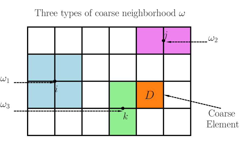
In practice, the extension ℋ⁡(v)\mathcal{H}({v}) is the numerical solution of the equation in the fine-scale finite element space Vh​(D)×Wh​(D){V}_{h}(D)\times W_{h}(D), where DD is a coarse block (see Fig. (1) for an illustration of coarse block and coarse neighborhood). This computation can be efficiently performed due to the moderated size of the coarse regions. Besides, the computations can be carried out in parallel, if the computations are required over all coarse regions.

Now we are ready to state the detailed construction of the offline velocity space VoffV^{\text{off}}. Our construction consists of the following three steps. We defer the analysis of the resulting GMsFEM method to Section 5.

Step 1: Building multiscale partition of unity functions.

First we introduce a set of generalized global partition of unity functions on the coarse grid. We denote the set of all coarse edges by ℰH\mathcal{E}_{H}, and consider the following finite element space:

MH:={v∈C0(ℰH):v|F∈P2(F), for all F∈ℰH}.M_{H}:=\{{v}\in C^{0}(\mathcal{E}_{H}):\ \ {v}|_{F}\in P^{2}(F),\quad\mbox{ for all }F\in\mathcal{E}_{H}\}.

Let 𝒫H\mathcal{P}_{H} be the set of the shape functions of the space MHM_{H}. Then 𝒫H\mathcal{P}_{H} also forms a partition of unity functions over the skeleton ℰH\mathcal{E}_{H}.

Next we introduce the set of multicale partition of unity functions for a two-dimensional domain Ω\Omega. We remark that the construction for the three-dimensional case is similar. For any χ∈𝒫H\chi\in\mathcal{P}_{H}, let ω\omega denote the support of χ\chi, and we call ω\omega a coarse neighborhood associated with χ\chi. In Figure 1, we sketch all three possible types of the coarse neighborhood, ω1\omega_{1}, ω2\omega_{2} and ω3\omega_{3}, respectively. ω1\omega_{1} corresponds to partition of unity funtion χ\chi having nodal value 1 at the coarse node ii; ω2\omega_{2} represents the support of χ\chi valuing 1 at node jj, and ω3\omega_{3} stands for support of χ\chi equaling to 1 at node kk.

Refer to caption
Figure 1: Illustration of three types of coarse neighborhoods and coarse element: ω1\omega_{1}, ω2\omega_{2} and ω3\omega_{3} denote the support of partition of unity functions χ\chi.

For each χ∈𝒫H\chi\in\mathcal{P}_{H}, we have two Brinkman extensions of χ\chi: ℋ⁡(χx)​ and ​ℋ​(χy)\mathcal{H}({\chi}^{x})\text{ and }\mathcal{H}({\chi}^{y}). Here ℋ⁡(χx)\mathcal{H}({\chi}^{x}) is the Brinkman extension of the Dirichlet data χx=(χ,0){\chi}^{x}=(\chi,0), and it is defined on each coarse block D⊂ωD\subset\omega. The extension ℋ⁡(χy)\mathcal{H}({\chi}^{y}) is defined similarly, with χy=(0,χ){\chi}^{y}=(0,\chi). We note that these vector functions can be extended by 00 to the entire domain Ω\Omega, since χ\chi vanishes over ∂ω\partial\omega. Finally, the generated partition of unity functions associated with χ\chi is χx=12​(ℋ⁡(χx))x\chi_{x}=\frac{1}{2}(\mathcal{H}({\chi}^{x}))_{x}, χy=12​(ℋ⁡(χy))y\chi_{y}=\frac{1}{2}(\mathcal{H}({\chi}^{y}))_{y}, where (⋅)x(\cdot)_{x} and (⋅)y(\cdot)_{y} denote the first component and second component of a vector, respectively. Thus, for each χ∈𝒫H\chi\in\mathcal{P}_{H}, we generate two partition of unity functions supported on ω\omega. All these extensions together form a set of multiscale partition of unity functions, which are denoted by:

𝒫ext={χi}i=1Np,\mathcal{P}_{\text{ext}}=\{\chi_{i}\}^{N_{p}}_{i=1},

where NpN_{p} is the number of multiscale partition of unity functions. We note that the set 𝒫ext\mathcal{P}_{\text{ext}} does not have the default property of partition of unity over the domain Ω\Omega, but only over the skeleton ℰH\mathcal{E}_{H}, i.e.,

∑i=1Npχi≡1on ℰH.\sum_{i=1}^{N_{p}}\chi_{i}\equiv 1\quad\text{on $\mathcal{E}_{H}$.} (7)

Step 2: Constructing local snapshot space Vsnapω{V}^{\omega}_{\text{snap}}.

In this step, we construct the local snapshot spaces. Proceeding as before, for each χ∈𝒫e​x​t\chi\in\mathcal{P}_{ext}, we let ω\omega denote its support set, and call it the coarse neighborhood associated with χ\chi, which consists of either two or four coarse blocks, cf. Figure 1. The construction of the local snapshots is further divided into two substeps: generating the snapshot space over all coarse neighborhoods ω\omega and then improving their linear independence.

Step 2.1. Computing snapshots: For each coarse neighborhood ω\omega, let Jh​(∂ω)\textsl{J}_{h}(\partial\omega) denote the set of fine nodes on ∂ω\partial\omega. Let δk∈C0​(∂ω)\delta_{k}\in C^{0}(\partial\omega) denote the shape function associated with the node xk∈Jh​(∂ω)x_{k}\in\textsl{J}_{h}(\partial\omega). i.e., δk∈C0​(∂ω)\delta_{k}\in C^{0}(\partial\omega) is the piecewise linear function that takes value 11 on the node xkx_{k} and vanishes on all other nodes. For each δk\delta_{k}, it generates two Brinkman extensions:

ψk,x=ℋ⁡((δk,0))andψk,y=ℋ⁡((0,δk)).{\psi}_{k,x}=\mathcal{H}((\delta_{k},0))\quad\mbox{and}\quad{\psi}_{k,y}=\mathcal{H}((0,\delta_{k})).

Now the raw snapshot space on ω\omega is given by

V~snapω=span{ψi,x,ψi,y:for allxi∈Jh(∂ω)}+span{(1,0),(0,1)}.\widetilde{{V}}^{\omega}_{\text{snap}}=\text{span}\{{\psi}_{i,x},{\psi}_{i,y}:\;\text{for all}\;x_{i}\in\textsl{J}_{h}(\partial\omega)\}+\text{span}\{(1,0),(0,1)\}.

Here we artificially add two constant vectors in the basis; see Remark 3.3 below for the discussions.

Step 2.2: Improving linear independence of snapshots: After obtaining a family of local functions for each coarse neighborhood, we need to discard the possible linearly dependent local snapshots. To this end, we use a spectral problem based on the Euclidian inner product. Specifically, Let UU be a matrix with columns being the local snapshots vector representation. We extract the important modes of UU through the spectral decomposition of UT​UU^{T}U. In this manner, we keep the linearly independent snapshots for each coarse neighborhood ω\omega and denote the resulting space by

Vsnapω=span​{ψlω,snap:1≤l≤Lω},{V}_{\text{snap}}^{\omega}=\text{span}\{{\psi}_{l}^{\omega,\text{snap}}:1\leq l\leq L^{\omega}\},

with LωL^{\omega} being the number of local basis functions for the coarse neighborhood ω\omega.

Step 3: Building the offline space Voff{V}^{\text{off}}.

In this final step, we build the global offline space Voff{V}^{\text{off}} from the snapshot spaces Vsnapω{V}^{\omega}_{\text{snap}}, and it involves two substeps: constructing local offline space and constructing global offline space.

Step 3.1: Local multiscale space V~offω\widetilde{{V}}^{\omega}_{\text{off}}. The idea at this step is to extract only important information from the computed local snapshots VsnapωV_{\text{snap}}^{\omega} corresponding to each coarse neighborhood ω\omega. This can be achieved by performing a dimension reduction procedure in the space Vsnapω{V}_{\text{snap}}^{\omega}. Namely, we consider the following spectral eigenvalue problem:

A​Ψ^kω,off=λk​S​Ψ^kω,off,\displaystyle A\widehat{{\Psi}}_{k}^{\omega,\text{off}}=\lambda_{k}S\widehat{{\Psi}}_{k}^{\omega,\text{off}}, (8)

where the matrices AA and SS are defined by

A\displaystyle\displaystyle A =[am​n]=∫ωκ(x)∇ψmω,snap⋅∇ψnω,snap, 1≤m,n≤Lω\displaystyle=[a_{mn}]=\int_{\omega}\kappa(x)\nabla{\psi}_{m}^{\omega,\text{snap}}\cdot\nabla{\psi}_{n}^{\omega,\text{snap}},\ 1\leq m,n\leq L^{\omega}
S\displaystyle\displaystyle S =[sm​n]=∫ωκ(x)ψmω,snapψnω,snap, 1≤m,n≤Lω.\displaystyle=[s_{mn}]=\int_{\omega}\kappa(x){\psi}_{m}^{\omega,\text{snap}}{\psi}_{n}^{\omega,\text{snap}},\ 1\leq m,n\leq L^{\omega}.

Then we reorder the eigenvalues λk\lambda_{k} are in an ascending order, and denote Ψ^kω,off\widehat{{\Psi}}_{k}^{\omega,\text{off}} as the coresponding eigenvectors.

To generate the offline space, we then choose the MoffM_{\text{off}} smallest eigenvalues of (8) and the corresponding eigenvectors in the respective space of snapshots by setting Ψ~kω,off=∑jΨ^k​joff​ψjω,snap\widetilde{{\Psi}}_{k}^{\omega,\text{off}}=\sum_{j}\widehat{\Psi}_{kj}^{\text{off}}\psi_{j}^{\omega,\text{snap}}, where Ψ^k​joff\widehat{\Psi}_{kj}^{\text{off}} are the coordinates of the vector Ψ^kω,off\widehat{{\Psi}}_{k}^{\omega,\text{off}}. We then construct the offline space V~offω\widetilde{{V}}_{\text{off}}^{\omega} corresponding to the coarse neighborhood ω\omega as

V~offω=span​(Ψ~1ω,,off,…,Ψ~Moffω,off).\widetilde{{V}}_{\text{off}}^{\omega}=\text{span}\left(\widetilde{{\Psi}}_{1}^{\omega,\text{,off}},\ldots,\widetilde{{\Psi}}_{M_{\text{off}}}^{\omega,\text{off}}\right).

We note that this step is performed only on each coarse neighborhood ω\omega. The dimensionality of the space V~offω\widetilde{{V}}^{\omega}_{\text{off}} solely depends on the eigenvalue problem (8) within the neighborhood ω\omega. It is known that this space is related to important features of the media (cf. [16]) such as high-conductivity channels and inclusions, and thus its dimensionality depends on the structure of the heterogeneities.

Remark 3.3.

In the construction of the local snapshot space, we have added constant functions in addition to spectral basis functions. Hence, the constant function, which is the eigenvectors corresponding to the zero eigenvalue of (8), will always be in the offline space. By the construction of the offline space, each offline space contains the partition of unity functions, and the smallest offline space consists of those partition of unity functions only. This will be crucial in the stability analysis of the methods in Section 5.

Step 3.2: Construction of the global offline space Voff{V}^{\text{off}} by partition of unity. The local multiscale spaces V~offω\widetilde{{V}}^{\omega}_{\text{off}} are defined only on each neighborhood ω\omega. However, it is not conforming if we simply extend the functions by 00 to the whole domain. We obtain a global conforming offline space VoffV^{\text{off}} as follows.

First, we multiply each local offline space V~offω\widetilde{{V}}^{\omega}_{\text{off}} by the corresponding partition of unity function χ\chi:

χ​V~offω=span​(χ​Ψ~1ω,off,…,χ​Ψ~Moffω,off).\chi\widetilde{{V}}^{\omega}_{\text{off}}=\text{span}\left(\chi\widetilde{{\Psi}}_{1}^{\omega,\text{off}},\ldots,\chi\widetilde{{\Psi}}_{M_{\text{off}}}^{\omega,\text{off}}\right).

Then the space χ​V~offω⊂H01​(ω)\chi\widetilde{{V}}^{\omega}_{\text{off}}\subset{H}^{1}_{0}(\omega), and we can extend the functions in χ​V~offω\chi\widetilde{V}^{\omega}_{\text{off}} to the whole domain Ω\Omega by zero, which is still denoted as χ​V~offω\chi\widetilde{{V}}^{\omega}_{\text{off}}. Finally, we need to make a correction of the divergence of the resulting functions to satisfy the following condition:

∇⋅Voff⊂Woff.\nabla\cdot{V}^{\text{off}}\subset W^{\text{off}}.

To this end, for each basis function χ​Ψ~iω,off\chi\widetilde{{\Psi}}_{i}^{\omega,\text{off}}, within each coarse block D⊂ωD\subset\omega, we keep its trace along ∂D\partial D and modify its interior values to be the Brinkman extension ℋ⁡(χ​Ψ~iω,o​f​f|∂D)\mathcal{H}(\chi\widetilde{{\Psi}}_{i}^{\omega,off}|_{\partial D}). We denote this modified space by ℋ⁡(χ​V~offω)\mathcal{H}(\chi\widetilde{{V}}^{\omega}_{\text{off}}). The global offline space VoffV^{\text{off}} results from assembling all these modified local spaces as:

Voff:={v∈(H01​(Ω))d:v|ω∈ℋ⁡(χ​V~offω)}.{V}^{\text{off}}:=\{{v}\in({H}^{1}_{0}(\Omega))^{d}:{v}|_{\omega}\in\mathcal{H}(\chi\widetilde{{V}}^{\omega}_{\text{off}})\}.

This completes the construction of the offline space Voff{V}^{\text{off}}. Finally, we refer to Section 2 for the coupling of the offline basis functions.

4 Numerical results

Now we test our framework with several examples. In our experiments, we take the domain Ω=[0,1]×[0,1]\Omega=[0,1]\times[0,1], the source term f=0f=0, and the boundary condition is the constant horizontal velocity:

g=(1,0)on∂Ω.{g}=(1,0)\quad\mbox{on}\quad\partial\Omega.

We study the model with different (inverse) permeability fields κ−1\kappa^{-1} depicted in Figure 2. Figure 2(a) shows a fast Darcy flow going through the slower region; in Figure 2(b), we exposit a slower Darcy flow past Darcy flow regions; in Figure 2(c), a free flow going across the Darcy flow region is represented; and in Figure 2(d), a Darcy flow passing the strong free flow region is shown.

Refer to caption Refer to caption
(a) Fast Darcy flow going through a slower region. (b) A slower Darcy flow past Darcy flow regions.
Refer to caption Refer to caption
(c) A free flow going across the Darcy flow region. (d) A Darcy flow passing the strong free flow region.
Figure 2: Four representative inverse permeability fields κ−1\kappa^{-1}.

We divide the computational domain Ω=[0 1]×[0 1]\Omega=[0\;1]\times[0\;1] into Nf=1/h2N_{f}=1/h^{2} equal squares (where each square is further divided into two triangles), and use P2/P0P_{2}/P_{0} elements on the fine mesh with h=1/100h=1/100. We use a coarse-mesh size H=1/10H=1/10 where we divide the domain Ω=[0,1]×[0,1]\Omega=[0,1]\times[0,1] into 1/H21/H^{2} squares.

We depict the fine-scale solution, and three coarse-scale solutions with coarse spaces of dimensions 798, 1110 and 2726 in Figure 3. The dimension of the fine scale velocity space VhV_{h} is 80802. In these numerical tests, we use the value of the permeability field κ−1\kappa^{-1} from Figure 2(a). We observe that a larger coarse space yields a better approximation of the fine-scale solution. Further, we have the following observations.

  • (a)

    The use of one single basis function for each node gives large errors and thus it is necessary to add spectral basis functions.

  • (b)

    The error decreases as more spectral basis functions are added in each coarse-grid block.

  • (c)

    The error decreases if the solution displays fast flow in some regions instead of Darcy flow over the whole region under the same contrast.

Refer to caption Refer to caption
(a) Fine-scale solution. (b) Coarse solution with solution space of 798.
Refer to caption Refer to caption
(c) Coarse solution with solution space of 1110. (d) Coarse solution with solution space of 2726.
Figure 3: The fine-scale solution and three coarse-scale solutions with different dimensions of coarse spaces using the permeability field κ−1\kappa^{-1} in Figure 2 (a).

In Tables 1-4, we present the results with the multiscale partition of unity functions as required by the conforming Galerkin formulation corresponding to permeability fields in Figure 2. In the tables, the first column shows the dimension of the offline space VoffV^{\text{off}}, and the L2L^{2}-weighted error between the offline solution uoffu^{\text{off}} and the fine-scale solution uu and the H1H^{1}-weighted energy error are calculated respectively by

‖u−uoff‖Lκ2​(D)=‖κ−1/2(u−uoff)‖L2​(Ω)‖κ−1/2u‖L2​(Ω)and‖u−uoff‖Hκ1​(D)=‖κ−1/2∇(u−uoff)‖L2​(Ω)‖κ−1/2∇u‖L2​(Ω).\|u-u^{\text{off}}\|_{L^{2}_{\kappa}(D)}=\frac{\left\|\kappa^{-1/2}(u-u^{\text{off}})\right\|_{L^{2}\left(\Omega\right)}}{\left\|\kappa^{-1/2}u\right\|_{L^{2}\left(\Omega\right)}}\quad\mbox{and}\quad\|u-u^{\text{off}}\|_{H^{1}_{\kappa}(D)}=\frac{\left\|\kappa^{-1/2}\nabla(u-u^{\text{off}})\right\|_{L^{2}\left(\Omega\right)}}{\left\|\kappa^{-1/2}\nabla u\right\|_{L^{2}\left(\Omega\right)}}.
Table 1: Numerical results for problem (1) with κ−1\kappa^{-1} in Figure 2(a). The L2L^{2}-weighted error and energy error are 66.34%66.34\% and 99.73%99.73\% for the MsFEM solution. In the simulation, the dimension of the snapshot space is fixed at 4498 with a weighted L2L^{2} and energy relative error 1.26%1.26\% and 2.13%2.13\%.
dim​(Voff)\text{dim}(V_{\text{off}}) ‖u−uoff‖\|u-u^{\text{off}}\| (%)
Lκ2​(D)\hskip 22.76228ptL^{2}_{\kappa}(D)\hskip 22.76228pt Hκ1​(D)\hskip 22.76228ptH^{1}_{\kappa}(D)\hskip 22.76228pt
888888 35.4635.46 74.9174.91
13721372 26.6226.62 58.2558.25
20282028 11.7911.79 26.0526.05
22042204 8.618.61 19.4719.47

In Table 1, we display the velocity error results using a permeability field with values of κ−1\kappa^{-1} large in the background, with smalle inclusions values, cf. Figure 2(a). For simplicity, we set a threshold value λoff\lambda^{\text{off}} for selecting eigenvectors in the construction of the offline space. Specifically, for each coarse neighborhood ω\omega, the offline space consists of those eigenvectors in Eqn (8) with eigenvalues λk≥λoff\lambda_{k}\geq\lambda^{\text{off}}. Notice that the smaller is λoff\lambda^{\text{off}}, the larger is the velocity offline space. In the simulation, the choices λoff=1/3, 1/4, 1/7, and 1/10\lambda^{\text{off}}=1/3\mbox{, }1/4\mbox{, }1/7\mbox{, and }1/10 give the offline spaces of dimension 888, 1372, 2028 and 2204, respectively. It is observed from Table 1 that the error decreases from 74.91%74.91\% to 19.47%19.47\%.

Table 2: Numerical results for problem (1) with κ−1\kappa^{-1} in Figure 2(b). The L2L^{2}-weighted error and energy error are 74.68%74.68\% and 130.42%130.42\% for the MsFEM solution. In the simulation, the dimension of the snapshot space is fixed at 4498 with a weighted L2L^{2} and energy relative error 1.33%1.33\% and 13.03%13.03\%.
dim​(Voff)\text{dim}(V_{\text{off}}) ‖u−uoff‖\|u-u^{\text{off}}\| (%)
Lκ2​(D)\hskip 22.76228ptL^{2}_{\kappa}(D)\hskip 22.76228pt Hκ1​(D)\hskip 22.76228ptH^{1}_{\kappa}(D)\hskip 22.76228pt
682682 7.867.86 36.9036.90
15121512 1.851.85 18.3718.37
22302230 1.511.51 15.2715.27
27442744 1.381.38 13.8413.84

The results in Table 2 are calculated with values of κ−1\kappa^{-1} that are large in inclusions, and small in the background, cf. Figure 2(b). Compared with results in Table 1, the errors in Table 2 are slightly better in the sense that the relative energy errors are smaller when using the same dimensional offline space. In this numerical test, we take λoff=1/3​, ​1/4​, ​1/7​, and ​1/10\lambda^{\text{off}}=1/3\mbox{, }1/4\mbox{, }1/7\mbox{, and }1/10 with the offline space of dimension 682, 1512, 2230 and 2744 respectively. From Table 2, the energy errors decrease from 36.90%36.90\% to 13.84%13.84\%.

Table 3: Numerical results for problem (1) with κ−1\kappa^{-1} in Figure 2(c). The L2L^{2}-weighted error and energy error are 85.25%85.25\% and 73.85%73.85\% for the MsFEM solution. In the simulation, the dimension of the snapshot space is fixed at 4498 with a weighted L2L^{2} and energy relative error 1.94%1.94\% and 3.54%3.54\%.
dim​(Voff)\text{dim}(V_{\text{off}}) ‖u−uoff‖\|u-u^{\text{off}}\| (%)
Lκ2​(D)\hskip 22.76228ptL^{2}_{\kappa}(D)\hskip 22.76228pt Hκ1​(D)\hskip 22.76228ptH^{1}_{\kappa}(D)\hskip 22.76228pt
834834 35.5835.58 38.1038.10
15121512 14.3414.34 19.4119.41
20842084 6.816.81 9.909.90
23062306 4.544.54 7.657.65

In Tables 3 and 4, we employ certain permeability fields κ−1\kappa^{-1} to get fast flow and Darcy flow simultaneously. In Table 3, we use a permeability field κ−1\kappa^{-1} small in inclusions, and large in the background, cf. Figure 2(c). In this numerical test, we take λoff=1/3​, ​1/4​, ​1/7​, and ​1/10\lambda^{\text{off}}=1/3\mbox{, }1/4\mbox{, }1/7\mbox{, and }1/10 with the offline space of dimension 834, 1512, 2084 and 2316 respectively. From Table 2, the energy errors decrease from 38.10%38.10\% to 7.65%7.65\%. In Table 4, we experimented with values of κ−1\kappa^{-1} large in inclusions, and small in the background as shown in Figure 2(d). In this numerical test, we take λoff=1/3​, ​1/4​, ​1/7​, and ​1/10\lambda^{\text{off}}=1/3\mbox{, }1/4\mbox{, }1/7\mbox{, and }1/10 with the offline space of dimension 682, 1090, 1992 and 3344 respectively. From Table 2, the energy errors decrease from 43.26%43.26\% to 5.38%5.38\%.

Table 4: Numerical results for problem (1) with κ−1\kappa^{-1} in Figure 2(d). The L2L^{2}-weighted error and energy error are 74.68%74.68\% and 130.42%130.42\% for the MsFEM solution. In the simulation, the dimension of the snapshot space is fixed at 4498 with a weighted L2L^{2} and energy relative error 1.47%1.47\% and 3.75%3.75\%.
dim​(Voff)\text{dim}(V_{\text{off}}) ‖u−uoff‖\|u-u^{\text{off}}\| (%)
Lκ2​(D)\hskip 22.76228ptL^{2}_{\kappa}(D)\hskip 22.76228pt Hκ1​(D)\hskip 22.76228ptH^{1}_{\kappa}(D)\hskip 22.76228pt
682682 46.8046.80 43.2643.26
10901090 30.9230.92 30.3030.30
19921992 13.4913.49 13.1513.15
33443344 6.366.36 5.385.38

In Table 3, the solution represents fast flow in the inclusions (with high permeability value) and Darcy flow in the background, whereas in Table 4, the solution is a fast flow in the background (with high permeability value) and Darcy flow in the inclusions. The results in these four tables indicate that the errors are smaller when fast flow exists.

5 Convergence analysis

In this section, we present a priori error estimates for the method. we first derive the stability argument. Then we show the approximation property of the method. For the sake of simplicity, we assume a homogeneous boundary condition g=0{g}=0 in the Brinkman equation (1).

5.1 Stability argument

To prove the stability of the method, we apply the well known inf-sup argument. First, we define a norm on V⁡(Ω){V}(\Omega) by

‖|u|‖V,Ω2=a⁡(u,u)+M​⟨div​u,div​u⟩Ω,{|\!|\!|{u}|\!|\!|}_{{\text{V},\Omega}}^{2}=a({u},{u})+M{\left\langle\mathrm{div}\,{u},\mathrm{div}\,{u}\right\rangle}_{\Omega}, (9)

and the norm on W⁡(Ω)W(\Omega) is defined by

‖|p|‖P,Ω=M−12​‖p‖L2​(Ω),{|\!|\!|p|\!|\!|}_{{\text{P},\Omega}}=M^{-\frac{1}{2}}\left\|p\right\|_{L^{2}\left(\Omega\right)}, (10)

where M=max⁡(‖κ−1‖L∞​(Ω), 1)M=\max(\left\|\kappa^{-1}\right\|_{L^{\infty}\left(\Omega\right)},\,1). We also define the following two null spaces:

Z\displaystyle{Z} :={v∈V(Ω):b(v,p)=0, for all p∈W(Ω)},\displaystyle:=\{{v}\in{V}(\Omega):\;b({v},p)=0,\quad\mbox{ for all }\;p\in W(\Omega)\},
Zoff\displaystyle{Z}^{\text{off}} :={v∈Voff:b(v,p)=0, for all p∈Woff}.\displaystyle:=\{{v}\in{V}^{\text{off}}:\;b({v},p)=0,\quad\mbox{ for all }\;p\in W^{\text{off}}\}.

Under these definitions and the construction of VoffV^{\text{off}} and WoffW^{\text{off}}, it holds:

Zoff⊂Z,a⁡(v,v)⪰‖|v|‖V,Ω for all ​v∈Z.{Z}^{\text{off}}\subset{Z},\quad a({v},{v})\succeq{|\!|\!|{v}|\!|\!|}_{{\text{V},\Omega}}\quad\mbox{ for all }{v}\in{Z}. (11)

Here, and in what follows, we use the notation A⪰BA\succeq B to represent A≥𝒞​BA\geq\mathcal{C}B with a constant 𝒞\mathcal{C} independent of the contrast and the functions involve, and a similar interpretation applies to the notation ⪯\preceq. The above two results imply that the bilinear form a⁡(⋅,⋅)a(\cdot,\cdot) is also coercive on Zoff{Z}^{\text{off}}.

We first verify that the continuous problem (1) satisfies the inf-sup condition.

Lemma 5.1.

Let |||⋅|||V,Ω{|\!|\!|\cdot|\!|\!|}_{{\text{V},\Omega}} and |||⋅|||P,Ω{|\!|\!|\cdot|\!|\!|}_{{\text{P},\Omega}} be defined in (9) and (10). Then the following inf-sup condition holds independent of the contrast

supv∈V⁡(Ω)\{0}⟨div​v,q⟩Ω‖|v|‖V,Ω⪰‖|q|‖P,Ω, for all ​q∈W⁡(Ω).\displaystyle\sup\limits_{{v}\in{V}(\Omega)\backslash\{0\}}\,\frac{{\left\langle\mathrm{div}\,{v},q\right\rangle}_{\Omega}}{{|\!|\!|{v}|\!|\!|}_{{\text{V},\Omega}}}\succeq{|\!|\!|q|\!|\!|}_{{\text{P},\Omega}},\,\mbox{ for all }q\in W(\Omega). (12)
Proof.

It is well known [3] that the operator b⁡(⋅,⋅)b(\cdot,\cdot) satisfies the inf-sup condition under the standard norms, i.e.,

supv∈V⁡(Ω)\{0}⟨div​v,q⟩Ω‖v‖H1​(Ω)⪰‖q‖L2​(Ω), for all ​q∈W⁡(Ω).\displaystyle\sup\limits_{{v}\in{V}(\Omega)\backslash\{0\}}\,\frac{{\left\langle\mathrm{div}\,{v},q\right\rangle}_{\Omega}}{\left\|{v}\right\|_{H^{1}\left(\Omega\right)}}\succeq\left\|q\right\|_{L^{2}\left(\Omega\right)},\,\mbox{ for all }q\in W(\Omega). (13)

By the definition of |||⋅|||V,Ω{|\!|\!|\cdot|\!|\!|}_{{\text{V},\Omega}} and |||⋅|||P,Ω{|\!|\!|\cdot|\!|\!|}_{{\text{P},\Omega}}, we have ‖|v|‖V,Ω≤M12​‖v‖H1​(Ω){|\!|\!|{v}|\!|\!|}_{{\text{V},\Omega}}\leq M^{\frac{1}{2}}\left\|{v}\right\|_{H^{1}\left(\Omega\right)}, and ‖q‖L2​(Ω)=M12​‖|q|‖P,Ω\left\|q\right\|_{L^{2}\left(\Omega\right)}=M^{\frac{1}{2}}{|\!|\!|q|\!|\!|}_{{\text{P},\Omega}} for all (v,q)∈V⁡(Ω)×W⁡(Ω)({v},q)\in{V}(\Omega)\times W(\Omega). Combining these facts with (13) completes the proof. ∎

Next, we show that the discrete problem (5) also satisfies this type of inf-sup condition with a constant independent of the contrast for every offline space Voff×Woff{V}^{\text{off}}\times W^{\text{off}}. First, we consider the following auxiliary space:

VH​(Ω)\displaystyle{V}_{H}(\Omega) :={v∈H1(Ω)|v|K∈Q2(K),∀K∈𝒯H},\displaystyle:=\{{v}\in{H}^{1}(\Omega)|\;{v}|_{K}\in{Q}^{2}(K),\;\forall K\in\mathcal{T}_{H}\},
WH​(Ω)\displaystyle W_{H}(\Omega) :={q∈L02(Ω)|q|K∈Q0(K),∀K∈𝒯H}.\displaystyle:=\{q\in L^{2}_{0}(\Omega)|\;q|_{K}\in{Q}^{0}(K),\;\forall K\in\mathcal{T}_{H}\}.

For the Brinkman equation, we have the following inf-sup condition in VH​(Ω)×WH​(Ω){V}_{H}(\Omega)\times W_{H}(\Omega) (see [2]),

supv∈VH​(Ω)\{0}⟨div​v,q⟩Ω‖v‖H1​(Ω)⪰‖q‖L2​(Ω), for all ​q∈WH​(Ω).\displaystyle\sup\limits_{{v}\in{V}_{H}(\Omega)\backslash\{0\}}\,\frac{{\left\langle\mathrm{div}\,{v},q\right\rangle}_{\Omega}}{\left\|{v}\right\|_{H^{1}\left(\Omega\right)}}\succeq\left\|q\right\|_{L^{2}\left(\Omega\right)},\,\mbox{ for all }q\in W_{H}(\Omega). (14)

Following the proof of Lemma 5.1, we can obtain the discrete inf-sup condition in VH​(Ω)×WH​(Ω){V}_{H}(\Omega)\times W_{H}(\Omega) with |||⋅|||V,Ω{|\!|\!|\cdot|\!|\!|}_{{\text{V},\Omega}} and |||⋅|||P,Ω{|\!|\!|\cdot|\!|\!|}_{{\text{P},\Omega}}, i.e.,

supv∈VH​(Ω)\{0}⟨div​v,q⟩Ω‖|v|‖V,Ω⪰‖|q|‖P,Ω, for all ​q∈WH​(Ω).\displaystyle\sup\limits_{{v}\in{V}_{H}(\Omega)\backslash\{0\}}\,\frac{{\left\langle\mathrm{div}\,{v},q\right\rangle}_{\Omega}}{{|\!|\!|{v}|\!|\!|}_{{\text{V},\Omega}}}\succeq{|\!|\!|q|\!|\!|}_{{\text{P},\Omega}},\,\mbox{ for all }q\in W_{H}(\Omega). (15)

To prove the inf-sup condition for the space Voff×Woff{V}^{\text{off}}\times W^{\text{off}}, we need the following result, which states the stability of the Brinkman extension with respect to the weighted norm defined in (9).

Lemma 5.2.

For any w∈(H1​(D))d{w}\in({H}^{1}(D))^{d}, the Brinkman extension ℋ⁡(w)\mathcal{H}({w}) of ww on DD satisfies

‖|ℋ⁡(w)|‖V,D⪯|‖w‖|V,D.\displaystyle{|\!|\!|\mathcal{H}({w})|\!|\!|}_{{\text{V},D}}\preceq{|\!|\!|{w}|\!|\!|}_{{\text{V},D}}. (16)
Proof.

By the definition of the Brinkman extension, (ℋ⁡(w),p)∈(H⁡(D))d×L02​(D)(\mathcal{H}({w}),p)\in({H}(D))^{d}\times L^{2}_{0}(D) satisfies

∇p−Δ​ℋ​(w)+κ−1​ℋ​(w)=0, in ​D,\displaystyle\nabla p-\Delta\mathcal{H}({w})+\kappa^{-1}\mathcal{H}({w})=0,\,\mbox{ in }D,
div​ℋ​(w)=∫∂Dw⋅n|D|​ in ​D,\displaystyle\mathrm{div}\,\,\mathcal{H}({w})=\frac{\int_{\partial D}{w}\cdot{n}}{|D|}\,\mbox{ in }D,
ℋ⁡(w)=w, on ​∂D.\displaystyle\mathcal{H}({w})={w},\,\mbox{ on }\partial D.

Denote v=ℋ⁡(w)−w{v}=\mathcal{H}({w})-{w}, then v{v} satisfies

∇p−Δ​v+κ−1​v=Δ​w−κ−1​w, in ​D,\displaystyle\nabla p-\Delta{v}+\kappa^{-1}{v}=\Delta{w}-\kappa^{-1}{w},\,\mbox{ in }D, (17)
div​v=∫∂Dw⋅n|D|−div​w​ in ​D,\displaystyle\mathrm{div}\,{v}=\frac{\int_{\partial D}{w}\cdot{n}}{|D|}-\mathrm{div}\,{w}\,\mbox{ in }D,
v=0, on ​∂D.\displaystyle{v}=0,\,\mbox{ on }\partial D.

Since p∈L02​(D)p\in L^{2}_{0}(D), by Lemma 11.2.3 in [2], there exists ϕ∈(H01​(D))d{\phi}\in({H}^{1}_{0}(D))^{d} such that

p=−div​ϕ and ‖ϕ‖H1​(D)⪯‖p‖L2​(D).\displaystyle p=-\mathrm{div}\,{\phi}\quad\mbox{ and }\quad\left\|{\phi}\right\|_{H^{1}\left(D\right)}\preceq\left\|p\right\|_{L^{2}\left(D\right)}. (18)

Multiplying Equation(17) by ϕ\phi and integrating by parts, we obtain,

⟨p,p⟩D+⟨∇v,∇ϕ⟩D+⟨κ−1​v,ϕ⟩D=−⟨∇w,∇ϕ⟩D−⟨κ−1​w,ϕ⟩D.{\left\langle p,\,p\right\rangle}_{D}+{\left\langle\nabla{v},\,\nabla{\phi}\right\rangle}_{D}+{\left\langle\kappa^{-1}{v},\,{\phi}\right\rangle}_{D}=-{\left\langle\nabla{w},\,\nabla{\phi}\right\rangle}_{D}-{\left\langle\kappa^{-1}{w},\,{\phi}\right\rangle}_{D}.

Thus

⟨p,p⟩D=−⟨∇v,∇ϕ⟩D−⟨κ−1​v,ϕ⟩D−⟨∇w,∇ϕ⟩D−⟨κ−1​w,ϕ⟩D.{\left\langle p,\,p\right\rangle}_{D}=-{\left\langle\nabla{v},\,\nabla{\phi}\right\rangle}_{D}-{\left\langle\kappa^{-1}{v},\,{\phi}\right\rangle}_{D}-{\left\langle\nabla{w},\,\nabla{\phi}\right\rangle}_{D}-{\left\langle\kappa^{-1}{w},\,{\phi}\right\rangle}_{D}.

Using the Cauchy-Schwarz inequality and (18), we arrive at,

‖p‖L2​(D)2\displaystyle\left\|p\right\|_{L^{2}\left(D\right)}^{2} ⪯(‖∇v‖L2​(D)+‖κ−1​v‖H−1​(D)+(‖∇w‖L2​(D)+‖κ−1​w‖H−1​(D))​‖p‖L2​(D)CLOSE\displaystyle\preceq(\left\|\nabla{v}\right\|_{L^{2}\left(D\right)}+\left\|\kappa^{-1}{v}\right\|_{H^{-1}(D)}+(\left\|\nabla{w}\right\|_{L^{2}\left(D\right)}+\left\|\kappa^{-1}{w}\right\|_{H^{-1}(D)})\left\|p\right\|_{L^{2}\left(D\right)}
⪯(‖∇v‖L2​(D)+M​‖κ−12​v‖L2​(D)+‖∇w‖L2​(D)+M​‖κ−12​w‖L2​(D))​‖p‖L2​(D).\displaystyle\preceq(\left\|\nabla{v}\right\|_{L^{2}\left(D\right)}+M\left\|\kappa^{-\frac{1}{2}}{v}\right\|_{L^{2}(D)}+\left\|\nabla{w}\right\|_{L^{2}\left(D\right)}+M\left\|\kappa^{-\frac{1}{2}}{w}\right\|_{L^{2}(D)})\left\|p\right\|_{L^{2}\left(D\right)}.

Then it yields the pressure estimate

‖p‖L2​(D)⪯\displaystyle\left\|p\right\|_{L^{2}\left(D\right)}\preceq ‖∇v‖L2​(D)+M​‖κ−12​v‖L2​(D)+‖∇w‖L2​(D)+M​‖κ−12​w‖L2​(D).\displaystyle\left\|\nabla{v}\right\|_{L^{2}\left(D\right)}+M\left\|\kappa^{-\frac{1}{2}}{v}\right\|_{L^{2}(D)}+\left\|\nabla{w}\right\|_{L^{2}\left(D\right)}+M\left\|\kappa^{-\frac{1}{2}}{w}\right\|_{L^{2}(D)}. (19)

Multiplying Equation(17) by v{v} and integrating by parts, yields,

−⟨p,div​v⟩D+⟨∇v,∇v⟩D+⟨κ−1​v,v⟩D=⟨Δ​w−κ−1​w,v⟩D.\displaystyle-{\left\langle p,\mathrm{div}\,{v}\right\rangle}_{D}+{\left\langle\nabla{v},\nabla{v}\right\rangle}_{D}+{\left\langle\kappa^{-1}{v},{v}\right\rangle}_{D}={\left\langle\Delta{w}-\kappa^{-1}{w},{v}\right\rangle}_{D}.

Using Cauchy-Schwarz inequality and the fact that pp has zero mean on DD, it follows that,

⟨∇v,∇v⟩D+⟨κ−1​v,v⟩D=⟨Δ​w−κ−1​w,v⟩D+⟨p,div​v⟩D\displaystyle{\left\langle\nabla{v},\nabla{v}\right\rangle}_{D}+{\left\langle\kappa^{-1}{v},{v}\right\rangle}_{D}={\left\langle\Delta{w}-\kappa^{-1}{w},{v}\right\rangle}_{D}+{\left\langle p,\mathrm{div}\,\,{v}\right\rangle}_{D}
=⟨Δ​w−κ−1​w,v⟩D+⟨p,div⁡(ℋ⁡(w)−w)⟩D\displaystyle={\left\langle\Delta{w}-\kappa^{-1}{w},{v}\right\rangle}_{D}+{\left\langle p,\mathrm{div}\,\,(\mathcal{H}({w})-{w})\right\rangle}_{D}
=⟨Δ​w−κ−1​w,v⟩D−⟨p,div​w⟩D\displaystyle={\left\langle\Delta{w}-\kappa^{-1}{w},{v}\right\rangle}_{D}-{\left\langle p,\mathrm{div}\,\,{w}\right\rangle}_{D}
≤‖∇w‖L2​(D)​‖∇v‖L2​(D)+‖κ−12​w‖L2​(D)​‖κ−12​v‖L2​(D)+‖p‖L2​(D)​‖div​w‖L2​(D).\displaystyle\leq\left\|\nabla{w}\right\|_{L^{2}\left(D\right)}\left\|\nabla{v}\right\|_{L^{2}\left(D\right)}+\left\|\kappa^{-\frac{1}{2}}{w}\right\|_{L^{2}\left(D\right)}\left\|\kappa^{-\frac{1}{2}}{v}\right\|_{L^{2}\left(D\right)}+\left\|p\right\|_{L^{2}\left(D\right)}\left\|\mathrm{div}\,{w}\right\|_{L^{2}\left(D\right)}.

Inserting the pressure estimate (19) and Young’s inequality, we deduce

⟨∇v,∇v⟩D+⟨κ−1​v,v⟩D\displaystyle{\left\langle\nabla{v},\nabla{v}\right\rangle}_{D}+{\left\langle\kappa^{-1}{v},{v}\right\rangle}_{D} ≤12​δ​(‖∇w‖L2​(D)2+‖κ−12​w‖L2​(D)2)+δ2​(‖∇v‖L2​(D)2+‖κ−12​v‖L2​(D)2)\displaystyle\leq\frac{1}{2\delta}(\left\|\nabla{w}\right\|_{L^{2}\left(D\right)}^{2}+\left\|\kappa^{-\frac{1}{2}}{w}\right\|_{L^{2}\left(D\right)}^{2})+\frac{\delta}{2}\left(\left\|\nabla{v}\right\|_{L^{2}\left(D\right)}^{2}+\left\|\kappa^{-\frac{1}{2}}{v}\right\|_{L^{2}\left(D\right)}^{2}\right)
+δ2​M​(‖∇v‖L2​(D)2+M​‖κ−12​v‖L2​(D)2+‖∇w‖L2​(D)2CLOSE\displaystyle+\frac{\delta}{2M}\left(\left\|\nabla{v}\right\|_{L^{2}\left(D\right)}^{2}+M\left\|\kappa^{-\frac{1}{2}}{v}\right\|_{L^{2}(D)}^{2}+\left\|\nabla{w}\right\|_{L^{2}\left(D\right)}^{2}\right.
OPEN+M​‖κ−12​w‖L2​(D)2)+M2​δ​‖div​w‖L2​(D)2.\displaystyle\left.+M\left\|\kappa^{-\frac{1}{2}}{w}\right\|_{L^{2}(D)}^{2}\right)+\frac{M}{2\delta}\left\|\mathrm{div}\,{w}\right\|_{L^{2}\left(D\right)}^{2}.

Now the choice δ=14\delta=\frac{1}{4} yields

⟨∇v,∇v⟩D+⟨κ−1​v,v⟩D⪯‖∇w‖L2​(D)2+‖κ−12​w‖L2​(D)2+M​‖div​w‖L2​(D)2=‖|w|‖V,D2.\displaystyle{\left\langle\nabla{v},\nabla{v}\right\rangle}_{D}+{\left\langle\kappa^{-1}{v},{v}\right\rangle}_{D}\preceq\left\|\nabla{w}\right\|_{L^{2}\left(D\right)}^{2}+\left\|\kappa^{-\frac{1}{2}}{w}\right\|_{L^{2}\left(D\right)}^{2}+M\left\|\mathrm{div}\,{w}\right\|_{L^{2}\left(D\right)}^{2}={|\!|\!|{w}|\!|\!|}_{{\text{V},D}}^{2}.

Recall that ℋ⁡(w)=v+w\mathcal{H}({w})={v}+{w}. By triangle inequality, we have

⟨∇ℋ​(w),∇ℋ​(w)⟩D+⟨κ−1​ℋ​(w),ℋ⁡(w)⟩D⪯‖|w|‖V,D2.\displaystyle{\left\langle\nabla\mathcal{H}({w}),\nabla\mathcal{H}({w})\right\rangle}_{D}+{\left\langle\kappa^{-1}\mathcal{H}({w}),\mathcal{H}({w})\right\rangle}_{D}\preceq{|\!|\!|{w}|\!|\!|}_{{\text{V},D}}^{2}.

It suffices to show

M12​‖div​ℋ​(w)‖L2​(D)⪯‖|w|‖V,D.\displaystyle M^{\frac{1}{2}}\left\|\mathrm{div}\,\mathcal{H}({w})\right\|_{L^{2}\left(D\right)}\preceq{|\!|\!|{w}|\!|\!|}_{{\text{V},D}}. (20)

Indeed from the compatibility condition, we obtain: div​ℋ​(w)=1|D|​∫Ddiv​w\mathrm{div}\,\mathcal{H}({w})=\frac{1}{|D|}\int\limits_{D}\,\mathrm{div}\,{w}. Hence,

|div​ℋ​(w)|=|1|D|​∫Ddiv​w|≤1|D|​∫D|div​w|≤‖div​w‖L2​(D)​|D|−12,\displaystyle|\mathrm{div}\,\mathcal{H}({w})|=|\frac{1}{|D|}\int\limits_{D}\,\mathrm{div}\,{w}|\leq\frac{1}{|D|}\int\limits_{D}\,|\mathrm{div}\,{w}|\leq\left\|\mathrm{div}\,{w}\right\|_{L^{2}\left(D\right)}|D|^{-\frac{1}{2}},

where in the last step we used Cauchy-Schwarz inequality. Consequently

‖div​ℋ​(w)‖L2​(D)2⪯‖div​w‖L2​(D)2​|D|−1​|D|=‖div​w‖L2​(D)2,\displaystyle\left\|\mathrm{div}\,\mathcal{H}({w})\right\|_{L^{2}\left(D\right)}^{2}\preceq\left\|\mathrm{div}\,{w}\right\|_{L^{2}\left(D\right)}^{2}|D|^{-1}|D|=\left\|\mathrm{div}\,{w}\right\|_{L^{2}\left(D\right)}^{2},

This completes the proof. ∎

We are now ready to show the inf-sup condition in the space Voff×Woff{V}^{\text{off}}\times W^{\text{off}}.

Lemma 5.3.

For |||⋅|||V,Ω{|\!|\!|\cdot|\!|\!|}_{{\text{V},\Omega}} and |||⋅|||P,Ω{|\!|\!|\cdot|\!|\!|}_{{\text{P},\Omega}} defined in (9) and (10), we have the following inf-sup condition with inf-sup constant independent of the contrast

supv∈Voff​(Ω)\{0}⟨div​v,q⟩Ω‖|v|‖V,Ω⪰‖|q|‖P,Ω, for all ​q∈Woff​(Ω).\displaystyle\sup\limits_{{v}\in{V}^{\text{off}}(\Omega)\backslash\{0\}}\frac{{\left\langle\mathrm{div}\,{v},q\right\rangle}_{\Omega}}{{|\!|\!|{v}|\!|\!|}_{{\text{V},\Omega}}}\succeq{|\!|\!|q|\!|\!|}_{{\text{P},\Omega}},\,\mbox{ for all }q\in W^{\mathrm{off}}(\Omega). (21)
Proof.

First note Woff=WH​(Ω)W^{\text{off}}=W_{H}(\Omega). By (15), we have

supv∈VH​(Ω)\{0}⟨div​v,q⟩Ω‖|v|‖V,Ω⪰‖|q|‖P,Ω, for all ​q∈Woff.\sup\limits_{{v}\in{V}_{H}(\Omega)\backslash\{0\}}\,\frac{\langle\mathrm{div}\ {v},q\rangle_{\Omega}}{{|\!|\!|{v}|\!|\!|}_{{\text{V},\Omega}}}\succeq{|\!|\!|q|\!|\!|}_{{\text{P},\Omega}},\,\mbox{ for all }q\in W^{\text{off}}.

For any v∈VH​(Ω){v}\in{V}_{H}(\Omega), let ℋ⁡(v)\mathcal{H}({v}) be the Brinkman extension of v|ℰH{v}|_{\mathcal{E}_{H}}, i.e., ℋ⁡(v)\mathcal{H}({v}) takes the value of v{v} on the skeleton ℰH\mathcal{E}_{H} and is extend to the interior by Brinkman extension within each coarse block. Then v|F∈[P2​(F)]2,∀F∈ℰH{v}|_{F}\in[P^{2}(F)]^{2},\;\forall F\in\mathcal{E}_{H}. According to the construction of the offline space Voff{V}^{\text{off}} in Section 3, we have

ℋ⁡(v)∈Voff.\mathcal{H}({v})\in{V}^{\text{off}}.

Moreover, for any q∈Woffq\in W^{\text{off}}, qq is piecewise constant on each coarse block. By combining this fact and the definition of Brinkman extension, we have

⟨div​v,q⟩D=⟨div​ℋ​(v),q⟩D,{\left\langle\mathrm{div}\,{v},q\right\rangle}_{D}={\left\langle\mathrm{div}\,\mathcal{H}({v}),q\right\rangle}_{D},

for every coarse block DD. Finally, we complete the proof by using Lemma 5.2:

‖|q|‖P,Ω\displaystyle{|\!|\!|q|\!|\!|}_{{\text{P},\Omega}} ⪯supv∈VH​(Ω)\{0}⟨div​v,q⟩Ω‖|v|‖V,Ω=supv∈VH​(Ω)\{0}⟨div​ℋ​(v),q⟩Ω‖|v|‖V,Ω\displaystyle\preceq\sup\limits_{{v}\in{V}_{H}(\Omega)\backslash\{0\}}\frac{{\left\langle\mathrm{div}\,{v},q\right\rangle}_{\Omega}}{{|\!|\!|{v}|\!|\!|}_{{\text{V},\Omega}}}=\sup\limits_{{v}\in{V}_{H}(\Omega)\backslash\{0\}}\frac{{\left\langle\mathrm{div}\,\mathcal{H}({v}),q\right\rangle}_{\Omega}}{{|\!|\!|{v}|\!|\!|}_{{\text{V},\Omega}}}
⪯supv∈VH​(Ω)\{0}⟨div​ℋ​(v),q⟩Ω‖|ℋ⁡(v)|‖V,Ω⪯supv∈Voff​(Ω)\{0}⟨div​v,q⟩Ω‖|v|‖V,Ω.\displaystyle\preceq\sup\limits_{{v}\in{V}_{H}(\Omega)\backslash\{0\}}\frac{{\left\langle\mathrm{div}\,\mathcal{H}({v}),q\right\rangle}_{\Omega}}{{|\!|\!|\mathcal{H}({v})|\!|\!|}_{{\text{V},\Omega}}}\preceq\sup\limits_{{v}\in{V}^{\text{off}}(\Omega)\backslash\{0\}}\frac{{\left\langle\mathrm{div}\,{v},q\right\rangle}_{\Omega}}{{|\!|\!|{v}|\!|\!|}_{{\text{V},\Omega}}}.

∎

Now by combining Lemma 5.1, Lemma 5.3 and (11), we obtain the following stability result, by repeating the proof of Theorem 3.2 in [26].

Theorem 5.4.

Let (u,p)∈V⁡(Ω)×W⁡(Ω)({u},p)\in{V}(\Omega)\times W(\Omega) and (u0,p0)∈Voff​(Ω)×Woff​(Ω)({u}_{0},p_{0})\in{V}^{\mathrm{off}}(\Omega)\times W^{\mathrm{off}}(\Omega) be the Galerkin solutions of problem (1) and problem (5) respectively. We have

‖|u−u0|‖V,Ω⪯infw∈Voff​(Ω)‖|u−w|‖V,Ω,\displaystyle{|\!|\!|{u}-{u}_{0}|\!|\!|}_{{\text{V},\Omega}}\preceq\inf\limits_{{w}\in{V}^{\text{off}}(\Omega)}{|\!|\!|{u}-{w}|\!|\!|}_{{\text{V},\Omega}}, (22)

5.2 Convergence results

Now we derive an error estimate for our method. To this end, we first give several basic estimates on the Brinkman extension.

Lemma 5.5.

For each partition of unity function χi\chi_{i} with support ωi\omega_{i}, let (uc,pc)∈(H1​(ωi))d×L02​(ωi)({u}_{c},p_{c})\in({H}^{1}(\omega_{i}))^{d}\times L^{2}_{0}(\omega_{i}) solve

∇pc−Δ​uc+\displaystyle\nabla p_{c}-\Delta{u}_{c}+ κ−1​uc\displaystyle\kappa^{-1}{u}_{c} =\displaystyle= 0\displaystyle 0 in ​ωi,\displaystyle\mbox{ in }\omega_{i},
div​uc\displaystyle\mathrm{div}\,{u}_{c} =\displaystyle= ∫∂ωig⋅n|ωi|\displaystyle\frac{\int_{\partial\omega_{i}}\,{g}\cdot n}{|\omega_{i}|} in ​ωi,\displaystyle\mbox{ in }\omega_{i},
uc\displaystyle\quad\;{u}_{c} =\displaystyle= g\displaystyle{g}  on ​∂ωi.\displaystyle\;\mbox{ on }\partial\omega_{i}.

Then the following a priori estimate holds

∫ωiχi2​|∇uc|2+∫ωiκ−1​χi2​|uc|2⪯∫ωi|∇χi|2​|uc|2+∫ωiκ−2​|uc|2+∫ωi|div​uc|2+‖pc‖L2​(ωi)2.\int_{\omega_{i}}\,\chi_{i}^{2}|\nabla{u}_{c}|^{2}+\int_{\omega_{i}}\,\kappa^{-1}\chi_{i}^{2}|{u}_{c}|^{2}\preceq\int_{\omega_{i}}\,|\nabla\chi_{i}|^{2}|{u}_{c}|^{2}+\int_{\omega_{i}}\,\kappa^{-2}|{u}_{c}|^{2}+\int_{\omega_{i}}\,{|\mathrm{div}\,{u}_{c}}|^{2}+\left\|p_{c}\right\|_{L^{2}\left(\omega_{i}\right)}^{2}. (23)
Proof.

Multiplying the equation by χi2​uc\chi_{i}^{2}{u}_{c} yields

−⟨pc,div⁡(χi2​uc)⟩ωi+⟨∇uc,∇(χi2​uc)⟩ωi+⟨κ−1​uc,χi2​uc⟩ωi=0.-{\left\langle p_{c},\mathrm{div}\,(\chi_{i}^{2}{u}_{c})\right\rangle}_{\omega_{i}}+{\left\langle\nabla{u}_{c},\nabla(\chi_{i}^{2}{u}_{c})\right\rangle}_{\omega_{i}}+{\left\langle\kappa^{-1}{u}_{c},\chi_{i}^{2}{u}_{c}\right\rangle}_{\omega_{i}}=0.

Some simple algebraic manipulations give

∫ωiχi2\displaystyle\int\limits_{\omega_{i}}\,\chi_{i}^{2} |∇uc|2+∫ωiκ−1χi2uc2=⟨pc,2χi∇χi⋅uc⟩ωi+⟨pc,χi2divuc⟩ωi−⟨∇uc,2χi∇χi⋅uc⟩ωi,\displaystyle|\nabla{u}_{c}|^{2}+\int\limits_{\omega_{i}}\,\kappa^{-1}\chi_{i}^{2}{u}_{c}^{2}={\left\langle p_{c},2\chi_{i}\nabla\chi_{i}\cdot{u}_{c}\right\rangle}_{\omega_{i}}+{\left\langle p_{c},\chi_{i}^{2}\mathrm{div}\,{u}_{c}\right\rangle}_{\omega_{i}}-{\left\langle\nabla{u}_{c},2\chi_{i}\nabla\chi_{i}\cdot{u}_{c}\right\rangle}_{\omega_{i}},
⪯‖pc‖L2​(ωi)(‖∇χi⋅uc‖L2​(ωi)+‖divuc‖L2​(ωi))+‖χi∇uc‖L2​(ωi)‖∇χi⋅uc‖L2​(ωi),\displaystyle\preceq\left\|p_{c}\right\|_{L^{2}\left(\omega_{i}\right)}(\left\|\nabla\chi_{i}\cdot{u}_{c}\right\|_{L^{2}\left(\omega_{i}\right)}+\left\|\mathrm{div}\,{u}_{c}\right\|_{L^{2}\left(\omega_{i}\right)})+\left\|\chi_{i}\nabla{u}_{c}\right\|_{L^{2}\left(\omega_{i}\right)}\left\|\nabla\chi_{i}\cdot{u}_{c}\right\|_{L^{2}\left(\omega_{i}\right)},
≤δ2(‖pc‖L2​(ωi)2+‖χi∇uc‖L2​(ωi)2)+12​δ(‖∇χi⋅uc‖L2​(ωi)2+‖divuc‖L2​(ωi)2).\displaystyle\leq\frac{\delta}{2}(\left\|p_{c}\right\|_{L^{2}\left(\omega_{i}\right)}^{2}+\left\|\chi_{i}\nabla{u}_{c}\right\|_{L^{2}\left(\omega_{i}\right)}^{2})+\frac{1}{2\delta}(\left\|\nabla\chi_{i}\cdot{u}_{c}\right\|_{L^{2}\left(\omega_{i}\right)}^{2}+\left\|\mathrm{div}\,{u}_{c}\right\|_{L^{2}\left(\omega_{i}\right)}^{2}).

Taking δ=14\delta=\frac{1}{4}, we obtain the desired inequality. ∎

Lemma 5.6.

Let ωi⊂𝒯H\omega_{i}\subset\mathcal{T}_{H} be an arbitrary coarse neighborhood. Let (uN,pN)∈(H01​(ωi))d×L02​(ωi)({u}_{N},p_{N})\in({H}^{1}_{0}(\omega_{i}))^{d}\times L^{2}_{0}(\omega_{i}) solve

∇pN−Δ​uN+\displaystyle\nabla p_{N}-\Delta{u}_{N}+ κ−1​uN\displaystyle\kappa^{-1}{u}_{N} =\displaystyle= f\displaystyle{f} in ​ωi,\displaystyle\mbox{ in }\omega_{i},
div​uN\displaystyle\mathrm{div}\,{u}_{N} =\displaystyle= 0\displaystyle 0 in ​ωi,\displaystyle\mbox{ in }\omega_{i},
uN\displaystyle\quad\;{u_{N}} =\displaystyle= 0\displaystyle 0 on ​∂ωi.\displaystyle\mbox{ on }\partial\omega_{i}.

Then there holds

‖|uN|‖V,ωi⪯H​‖f‖L2​(ωi).\displaystyle{|\!|\!|{u}_{N}|\!|\!|}_{{\text{V},\omega_{i}}}\preceq H\left\|{f}\right\|_{L^{2}\left(\omega_{i}\right)}. (24)
Proof.

By multiplying the first equation by uN{u}_{N}, integrating by parts and the divergence free property of uN{u}_{N}, we obtain

‖∇uN‖L2​(ωi)2+‖κ−12​uN‖L2​(ωi)2=⟨f,uN⟩ωi.\displaystyle\left\|\nabla{u}_{N}\right\|_{L^{2}\left(\omega_{i}\right)}^{2}+\left\|\kappa^{-\frac{1}{2}}{u}_{N}\right\|_{L^{2}(\omega_{i})}^{2}={\left\langle{f},\,{u}_{N}\right\rangle}_{\omega_{i}}.

In view of the boundary condition, we can apply Poincaré’s inequality,

‖uN‖L2​(ωi)⪯H​‖∇uN‖L2​(ωi).\left\|{u}_{N}\right\|_{L^{2}\left(\omega_{i}\right)}\preceq H\left\|\nabla{u}_{N}\right\|_{L^{2}\left(\omega_{i}\right)}.

Thus

‖∇uN‖L2​(ωi)2+‖κ−12​uN‖L2​(ωi)2=⟨f,uN⟩ωi⪯H​‖∇uN‖L2​(ωi)​‖f‖L2​(ωi).\displaystyle\left\|\nabla{u}_{N}\right\|_{L^{2}\left(\omega_{i}\right)}^{2}+\left\|\kappa^{-\frac{1}{2}}{u}_{N}\right\|_{L^{2}(\omega_{i})}^{2}={\left\langle{f},\,{u}_{N}\right\rangle}_{\omega_{i}}\preceq H\left\|\nabla{u}_{N}\right\|_{L^{2}\left(\omega_{i}\right)}\left\|{f}\right\|_{L^{2}\left(\omega_{i}\right)}.

Finally, we complete the proof by the young’s inequality. ∎

Now we are ready to state our main error estimate.

Theorem 5.7.

Let Λ∗=minωi⁡λLi+1ωi\Lambda_{*}=\min\limits_{\omega_{i}}\lambda^{\omega_{i}}_{L_{i}+1}. Then

‖|u−u0|‖V,Ω2⪯1Λ∗​‖∇u‖L2​(Ω)2+H2​‖f⁡(x)‖L2​(Ω)2+‖pc‖L2​(Ω)2.\displaystyle{|\!|\!|u-u_{0}|\!|\!|}_{{\text{V},\Omega}}^{2}\preceq\frac{1}{\Lambda_{*}}\left\|\nabla u\right\|_{L^{2}\left(\Omega\right)}^{2}+H^{2}\left\|f(x)\right\|_{L^{2}\left(\Omega\right)}^{2}+\left\|p_{c}\right\|_{L^{2}\left(\Omega\right)}^{2}.

where pcp_{c} is defined by (25) below.

Proof.

In view of the linearity of the equation (1), on each coarse neighborhood ωi⊂𝒯H\omega_{i}\subset\mathcal{T}_{H}, uu can be decomposed into u=ℋ⁡(u)+uNu=\mathcal{H}({u})+{u}_{N}, where ℋ⁡(u)\mathcal{H}({u}) is the Brinkman extension of u{u} and uN{u}_{N} is the residual in Lemma 5.6. For each χi\chi_{i}, let I0​uI^{0}{u} be the local interpolant of u{u} in the local offline space V~offωi\tilde{{V}}^{\omega_{i}}_{\text{off}}. Then there exists pc∈L2​(ωi)p_{c}\in L^{2}(\omega_{i}), s.t.

∇pc−Δ⁡(u−I0​u)+\displaystyle\nabla p_{c}-\Delta({u}-I^{0}{u})+ κ−1​(u−I0​u)\displaystyle\kappa^{-1}({u}-I^{0}{u}) =\displaystyle= 0\displaystyle 0 in ​ωi,\displaystyle\mbox{ in }\omega_{i}, (25)
div⁡(u−I0​u)\displaystyle\mathrm{div}\,({u}-I^{0}{u}) =\displaystyle= ∫∂ωihi⋅n|ωi|\displaystyle\frac{\int_{\partial\omega_{i}}\,{h_{i}}\cdot n}{|\omega_{i}|} in ​ωi,\displaystyle\mbox{ in }\omega_{i},
(u−I0​u)\displaystyle\quad\;({u}-I^{0}{u}) =\displaystyle= hi\displaystyle{h_{i}}  on ​∂ωi,\displaystyle\;\mbox{ on }\partial\omega_{i},

since I0​uI^{0}{u} equals 0 over ∂ωi\partial\omega_{i} (the support of χi\chi_{i} is ωi\omega_{i}) and each basis in V~offωi\tilde{{V}}^{\omega_{i}}_{\text{off}} has the properties of divergence constant. Here, hih_{i} denotes the boundary value of u−I0​u{u}-I^{0}{u} over ∂ωi\partial\omega_{i}.

By the construction of the offline space VoffV^{\text{off}}, ℋ⁡(χi​I0​u)∈Voff\mathcal{H}(\chi_{i}I^{0}{u})\in{V}^{\text{off}}. By Theorem 5.4, we have

‖|u−u0|‖V,Ω2\displaystyle{|\!|\!|{u}-{u_{0}}|\!|\!|}_{{\text{V},\Omega}}^{2} ⪯infv∈Voff‖|u−v|‖V,Ω2\displaystyle\preceq\inf\limits_{{v}\in{V}^{\text{off}}}\,{|\!|\!|{u}-{v}|\!|\!|}_{{\text{V},\Omega}}^{2}
⪯‖|u−∑i=1NCℋ⁡(χi​I0​u)|‖V,Ω2⪯|‖ℋ⁡(u)−∑i=1Ncℋ⁡(χi​I0​u)‖|V,Ω2+|​‖uN‖|V,Ω2,\displaystyle\preceq{\bigg|\!\bigg|\!\bigg|{u}-\sum^{N_{C}}_{i=1}\mathcal{H}(\chi_{i}I^{0}{u})\bigg|\!\bigg|\!\bigg|\;}_{{\text{V},\Omega}}^{2}\preceq{\bigg|\!\bigg|\!\bigg|\mathcal{H}({u})-\sum^{N_{c}}_{i=1}\mathcal{H}(\chi_{i}I^{0}{u})\bigg|\!\bigg|\!\bigg|\;}_{{\text{V},\Omega}}^{2}+{|\!|\!|{u}_{N}|\!|\!|}_{{\text{V},\Omega}}^{2},
⪯‖|ℋ⁡(∑i=1Ncχi​u)−∑i=1Ncℋ⁡(χi​I0​u)|‖V,Ω2+H2​‖f⁡(x)‖L2​(ωi)2.\displaystyle\preceq{\bigg|\!\bigg|\!\bigg|\mathcal{H}(\sum^{N_{c}}_{i=1}\chi_{i}{u})-\sum^{N_{c}}_{i=1}\mathcal{H}(\chi_{i}I^{0}{u})\bigg|\!\bigg|\!\bigg|\;}_{{\text{V},\Omega}}^{2}+H^{2}\left\|f(x)\right\|_{L^{2}\left(\omega_{i}\right)}^{2}.

Here the last step follows from the estimate in Lemma 5.6. For the first term, we have

|||ℋ(∑i=1Ncχiu)−∑i=1Ncℋ(χiI0u)|||V,Ω2=|||ℋ(∑i=1Nc(χiu−χiI0u)|||V,Ω2\displaystyle{\bigg|\!\bigg|\!\bigg|\mathcal{H}(\sum^{N_{c}}_{i=1}\chi_{i}{u})-\sum^{N_{c}}_{i=1}\mathcal{H}(\chi_{i}I^{0}{u})\bigg|\!\bigg|\!\bigg|\;}_{{\text{V},\Omega}}^{2}={\bigg|\!\bigg|\!\bigg|\mathcal{H}(\sum^{N_{c}}_{i=1}(\chi_{i}{u}-\chi_{i}I^{0}{u})\bigg|\!\bigg|\!\bigg|\;}_{{\text{V},\Omega}}^{2}
⪯∑i=1Nc‖|ℋ⁡(χi​u−χi​I0​u)|‖V,ωi2⪯∑i=1Nc‖|χi​(u−I0​u)|‖V,ωi2,\displaystyle\preceq\sum_{i=1}^{N_{c}}{|\!|\!|\mathcal{H}(\chi_{i}{u}-\chi_{i}I^{0}{u})|\!|\!|}_{{\text{V},\omega_{i}}}^{2}\preceq\sum_{i=1}^{N_{c}}{|\!|\!|\chi_{i}({u}-I^{0}{u})|\!|\!|}_{{\text{V},\omega_{i}}}^{2},

where at the last step we have applied Lemma 5.2 on each coarse neighborhood ωi\omega_{i}. Consequently,

‖|u−u0|‖V,Ω2\displaystyle{|\!|\!|{u}-{u}_{0}|\!|\!|}_{{\text{V},\Omega}}^{2} ⪯∑i=1Nc‖|χi​(u−I0​u)|‖V,ωi2+H2​‖f‖L2​(ωi)2\displaystyle\preceq\sum\limits_{i=1}^{N_{c}}{|\!|\!|\chi_{i}({u}-I^{0}{u})|\!|\!|}_{{\text{V},\omega_{i}}}^{2}+H^{2}\left\|{f}\right\|_{L^{2}\left(\omega_{i}\right)}^{2}
⪯∑i=1Nc∫ωiχi2​|∇(u−I0​u)|2+∫ωiκ−1​χi2​|u−I0​u|2\displaystyle\preceq\sum\limits^{N_{c}}_{i=1}\int\limits_{\omega_{i}}\,\chi_{i}^{2}|\nabla({u}-I^{0}{u})|^{2}+\int\limits_{\omega_{i}}\,\kappa^{-1}\chi_{i}^{2}|{u}-I^{0}{u}|^{2}
+M∫ωiχi2|div(u−I0u)|2+M∫ωi|∇χi|2|u−I0u|2+H2‖f‖L2​(ωi)2.\displaystyle+M\int\limits_{\omega_{i}}\,\chi_{i}^{2}|\mathrm{div}\,({u}-I^{0}{u})|^{2}+M\int\limits_{\omega_{i}}|\nabla\chi_{i}|^{2}|{u}-I^{0}{u}|^{2}+H^{2}\left\|{f}\right\|_{L^{2}\left(\omega_{i}\right)}^{2}.

By applying Lemma 5.5 to the term u−I0​u{u}-I^{0}{u} in Eqn. (25), we deduce

‖|u−u0|‖V,Ω2⪯\displaystyle{|\!|\!|{u}-{u}_{0}|\!|\!|}_{{\text{V},\Omega}}^{2}\preceq ∑iM​∫ωi|∇χi|2​|u−I0​u|2+∫ωi(κ−1)2​|u−I0​u|2\displaystyle\sum\limits_{i}M\int_{\omega_{i}}|\nabla\chi_{i}|^{2}|{u}-I^{0}{u}|^{2}+\int_{\omega_{i}}\,(\kappa^{-1})^{2}|{u}-I^{0}{u}|^{2}
+M∫ωiχi2|div(u−I0u)|2+H2‖f‖L2​(ωi)2+‖pc‖L2​(ωi)2.\displaystyle+M\int_{\omega_{i}}\,\chi_{i}^{2}|\mathrm{div}\,{({u}-I^{0}{u})}|^{2}+H^{2}\left\|{f}\right\|_{L^{2}\left(\omega_{i}\right)}^{2}+\left\|p_{c}\right\|_{L^{2}\left(\omega_{i}\right)}^{2}.

Finally, using the spectral problem (8), with AA and SS defined by

A\displaystyle\displaystyle A =[am​n]=∫ωi(χi)2∇ψmω,snap⋅∇ψnω,snap,\displaystyle=[a_{mn}]=\int_{\omega_{i}}(\chi_{i})^{2}\nabla{\psi}_{m}^{\omega,\text{snap}}\cdot\nabla{\psi}_{n}^{\omega,\text{snap}}, (26)
S\displaystyle\displaystyle S =[sm​n]=∫ωi(κ​(x)−2+M​(∇χi)2)​ψmω,snap⋅ψnω,snap+M​∫ωi(χi)2​div​ψmω,snap​div​ψnω,snap,\displaystyle=[s_{mn}]=\int_{\omega_{i}}(\kappa(x)^{-2}+M(\nabla\chi_{i})^{2}){\psi}_{m}^{\omega,\text{snap}}\cdot{\psi}_{n}^{\omega,\text{snap}}+M\int_{\omega_{i}}(\chi_{i})^{2}\mathrm{div}\,{\psi}_{m}^{\omega,\text{snap}}\mathrm{div}\,{\psi}_{n}^{\omega,\text{snap}},

we have

∫ωiM​(∇χi)2​|u−I0​u|2+∫ωi(κ−1)2​|u−I0​u|2+M​∫ωi(χi)2​|div⁡(u−I0​u)|2\displaystyle\int_{\omega_{i}}\,M(\nabla\chi_{i})^{2}|{u}-I^{0}{u}|^{2}+\int_{\omega_{i}}\,(\kappa^{-1})^{2}|{u}-I^{0}{u}|^{2}+M\int_{\omega_{i}}\,(\chi_{i})^{2}|\mathrm{div}\,{({u}-I^{0}{u})}|^{2}
≤1λLi+1ωi​∫ωi(χi)2​|∇(u−I0​u)|2.\displaystyle\leq\frac{1}{\lambda^{\omega_{i}}_{L_{i}+1}}\int_{\omega_{i}}\,(\chi_{i})^{2}|\nabla({u}-I^{0}{u})|^{2}.

Hence,

‖|u−u0|‖V,Ω2⪯∑i1λLi+1ωi​∫ωi(χi)2​|∇(u−I0​u)|2+H2​‖f⁡(x)‖L2​(ωi)2+‖pc‖L2​(ωi)2.\displaystyle{|\!|\!|u-u_{0}|\!|\!|}_{{\text{V},\Omega}}^{2}\preceq\sum\limits_{i}\frac{1}{\lambda^{\omega_{i}}_{L_{i}+1}}\int_{\omega_{i}}\,(\chi_{i})^{2}|\nabla(u-I^{0}u)|^{2}+H^{2}\left\|f(x)\right\|_{L^{2}\left(\omega_{i}\right)}^{2}+\left\|p_{c}\right\|_{L^{2}\left(\omega_{i}\right)}^{2}.

Upon denoting Λ∗=minωi⁡λLi+1ωi\Lambda_{*}=\min\limits_{\omega_{i}}\lambda^{\omega_{i}}_{L_{i}+1}, we deduce

‖|u−u0|‖V,Ω2⪯1Λ∗​∑i∫ωi(χi)2​|∇(u−I0​u)|2+H2​‖f⁡(x)‖L2​(ωi)2+‖pc‖L2​(ωi)2.\displaystyle{|\!|\!|u-u_{0}|\!|\!|}_{{\text{V},\Omega}}^{2}\preceq\frac{1}{\Lambda_{*}}\sum\limits_{i}\int_{\omega_{i}}\,(\chi_{i})^{2}|\nabla(u-I^{0}u)|^{2}+H^{2}\left\|f(x)\right\|_{L^{2}\left(\omega_{i}\right)}^{2}+\left\|p_{c}\right\|_{L^{2}\left(\omega_{i}\right)}^{2}.

Using the inequality ‖∇I0u‖L2​(ωi)⪯‖∇u‖L2​(ωi)\left\|\nabla I^{0}u\right\|_{L^{2}\left(\omega_{i}\right)}\preceq\left\|\nabla u\right\|_{L^{2}\left(\omega_{i}\right)},

‖|u−u0|‖V,Ω2⪯1Λ∗​∑i‖∇u‖L2​(ωi)2+H2​‖f⁡(x)‖L2​(ωi)2+‖pc‖L2​(ωi)2,\displaystyle{|\!|\!|u-u_{0}|\!|\!|}_{{\text{V},\Omega}}^{2}\preceq\frac{1}{\Lambda_{*}}\sum\limits_{i}\left\|\nabla u\right\|_{L^{2}\left(\omega_{i}\right)}^{2}+H^{2}\left\|f(x)\right\|_{L^{2}\left(\omega_{i}\right)}^{2}+\left\|p_{c}\right\|_{L^{2}\left(\omega_{i}\right)}^{2},

and thus

‖|u−u0|‖V,Ω2⪯1Λ∗​‖∇u‖L2​(Ω)2+H2​‖f⁡(x)‖L2​(Ω)2+‖pc‖L2​(Ω)2.\displaystyle{|\!|\!|u-u_{0}|\!|\!|}_{{\text{V},\Omega}}^{2}\preceq\frac{1}{\Lambda_{*}}\left\|\nabla u\right\|_{L^{2}\left(\Omega\right)}^{2}+H^{2}\left\|f(x)\right\|_{L^{2}\left(\Omega\right)}^{2}+\left\|p_{c}\right\|_{L^{2}\left(\Omega\right)}^{2}.

This completes the proof of the theorem. ∎

Remark 5.8.

We note that in the analysis, we have used the spectral problem (26), instead of (8) in the numerical simulation. In view of the inequality ‖div​u‖L2​(D)≤‖∇u‖L2​(D)\left\|\mathrm{div}\,u\right\|_{L^{2}\left(D\right)}\leq\left\|\nabla u\right\|_{L^{2}\left(D\right)} for any u∈(H1​(D))du\in(H^{1}(D))^{d} and the fact that χi\chi_{i} is bounded, these two spectral problems are equivalent provided that MM is bounded. Hence our analysis does provide partial justification for the algorithm. The constant MM appears as a result of the definition of the velocity and pressure norms, cf. (9) and (10), which is needed for the inf-sup condition. It remains unclear how to get rid of the constant MM in the norm definition in the convergence analysis.

6 Conclusion

In this work, we have developed a mixed generalized multiscale finite element method for the Brinkman flow in high-contrast media, which is able to capture both the Stokes flow and the Darcy flow in respective regions. In the fine grid, we approximate the velocity and pressure with piecewise quadratic and piecewise constant functions. We develop a novel approach to construct a coarse approximation for the velocity snapshot space, and a robust low-dimensional offline space for the velocity. The stability of the mixed GMsFEM and a priori error estimates are derived. The two-dimensional numerical examples illustrate clearly the robustness and efficiency of the method.

In our discussion, we have focused on the approximation of the velocity space, and simply taken the piecewise constant space for the pressure. This may not be the best choice, as can be seen from Thm 5.7. The mixed finite element space may get better results with a better pressure space and accordingly an enriched velocity space. We leave the enriching of pressure space to a future work. Further, it is natural to extend the proposed method to the Stokes model in perforated domains.

7 Acknowledgements

G. Li’s research is partially supported by DOE.

References

  • [1] T. Arbogast, Analysis of a two-scale, locally conservative subgrid upscaling for elliptic problems, SIAM J. Numer. Anal., 42 (2004), pp. 576–598 (electronic).
  • [2] S. Brenner and L. Scott, The Mathematical Theory of Finite Element Methods, Springer-Verlag, New York, 2007.
  • [3] F. Brezzi and M. Fortin, Mixed and hybrid finite element methods, Springer-Verlag, Berlin - Heidelberg - New York, 1991.
  • [4] D. Brown, Y. Efendiev, G. Li, and V. Savatorova, Homogenization of high-contrast brinkman flows. submitted, 2013.
  • [5] C.-C. Chu, I. G. Graham, and T.-Y. Hou, A new multiscale finite element method for high-contrast elliptic interface problems, Math. Comp., 79 (2010), pp. 1915–1955.
  • [6] E. Chung and Y. Efendiev, Reduced-contrast approximations for high-contrast multiscale flow problems, Multiscale Model. Simul., 8 (2010), pp. 1128–1153.
  • [7] E. Chung, Y. Efendiev, and R. Gibson, An energy-conserving discontinuous multiscale finite element method for the wave equation in heterogeneous media, Advances in Adaptive Data Analysis, 3 (2011), pp. 251–268.
  • [8] E. Chung, Y. Efendiev, and W. T. Leung, Generalized multiscale finite element method for wave propagation in heterogeneous media, preprint, available as arXiv:1307.0123, (2013).
  • [9] E. Chung and W. T. Leung, A sub-grid structure enhanced discontinuous galerkin method for multiscale diffusion and convection-diffusion problems, Communications in Computational Physics, 14 (2013), pp. 370–392.
  • [10] L. Durlofsky, Numerical calculation of equivalent grid block permeability tensors for heterogeneous porous media, Water Resour. Res., 27 (1991), pp. 699–708.
  • [11] L. Durlofsky and J. F. Brady, Analysis of the brinkman equation as a model for flow in porous media, Phys. Fluids, 30 (1987), pp. 3329–3341.
  • [12] W. E and B. Engquist, Heterogeneous multiscale methods, Comm. Math. Sci., 1 (2003), pp. 87–132.
  • [13] Y. Efendiev, J. Galvis, and T. Hou, Generalized multiscale finite element methods, Journal of Computational Physics, 251 (2013), pp. 116–135.
  • [14] Y. Efendiev, J. Galvis, R. Lazarov, and J. Willems, Robust domain decomposition preconditioners for abstract symmetric positive definite bilinear forms, ESAIM: Mathematical Modelling and Numerical Analysis.
  • [15] Y. Efendiev, J. Galvis, and F. Thomines, A systematic coarse-scale model reduction technique for parameter-dependent flows in highly heterogeneous media and its applications, Multiscale Model. Simul., 10 (2012), pp. 1317–1343.
  • [16] Y. Efendiev, J. Galvis, and X. Wu, Multiscale finite element methods for high-contrast problems using local spectral basis functions, Journal of Computational Physics, 230 (2011), pp. 937–955.
  • [17] Y. Efendiev and T. Hou, Multiscale Finite Element Methods: Theory and Applications, vol. 4 of Surveys and Tutorials in the Applied Mathematical Sciences, Springer, New York, 2009.
  • [18] Y. Efendiev, T. Hou, and V. Ginting, Multiscale finite element methods for nonlinear problems and their applications, Comm. Math. Sci., 2 (2004), pp. 553–589.
  • [19] M. Ghommem, M. Presho, V. M. Calo, and Y. Efendiev, Mode decomposition methods for flows in high-contrast porous media. global–-local approach, Journal of Computational Physics, 253, pp. 226––238.
  • [20] A. Gulbransen, V. Hauge, and K. Lie, A multiscale mixed finite-element method for vuggy and naturally-fractured reservoirs, NSCM-21.
  • [21] O. Iliev, R. Lazarov, and J. Willems, Variational multiscale finite element method for flows in highly porous media., Multiscale Modeling & Simulation, 9.4 (2011), pp. 1350–1372.
  • [22] A.-R. Khaleda and K. Vafai, The role of porous media in modeling flow and heat transfer in biological tissues, International Journal of Heat and Mass Transfer, 46(26) (2003), p. 4989 – 5003.
  • [23] P. Popov, G. Qin, L. Bi, Y. Efendiev, R. Ewing, Z. Kang, and J. Li, Multiscale methods for modeling fluid flow through naturally fractured carbonate karst reservoirs, in Proceedings of the SPE Annual Technical Conference and Exhibition, 2007. SPE 110778.
  • [24] F. J. Valdes-Parada, J. A. Ochoa-Tapia, and J. Alvarez-Ramirez, On the effective viscosity for the darcy–brinkman equation, Physica A: Statistical Mechanics and its Applications, 385(1) (2007), pp. 69 – 79.
  • [25] X. Wu, Y. Efendiev, and T. Hou, Analysis of upscaling absolute permeability, Discrete and Continuous Dynamical Systems, Series B., 2 (2002), pp. 158–204.
  • [26] X. Xie, J. Xu, and G. Xue, Uniformly-stable finite element methods for darcy-stokes-brinkman models, Journal of Computational Mathematics, 26 (2008), pp. 437–455.