Metabolic fluxes and value production
Abstract
Metabolic fluxes in cells are governed by physical, physiological, and economic principles. Here I assume an optimal allocation of enzyme resources and postulate a general principle for metabolism: each enzyme must convert less valuable into more valuable metabolites to justify its own cost. The “values”, called economic potentials, describe the individual contributions of metabolites to cell fitness. Local value production implies that the cost of an enzyme must be balanced by a benefit, given by the economic potential difference the catalysed reaction multiplied by the flux. Flux profiles that satisfy this principle – i.e. for which consistent potentials can be found – are called economical. Economical fluxes must lead from lower to higher economic potentials, so certain flux cycles are incompatible with any choice of economic potentials and can be excluded. To obtain economical flux profiles, non-beneficial local patterns, called futile motifs, can be systematically removed from a given flux distribution. The principle of local value production resembles thermodynamic principles and complements them in models. Here I describe a modelling framework called Value Balance Analysis (VBA) that uses the two principles and yields the same solution as enzyme cost minimisation (in kinetic models) and flux cost minimisation (in FBA). Given an economical flux distribution, kinetic models in enzyme-optimal states and with these fluxes can be constructed systematically. VBA justifies the principle of minimal fluxes and the exclusion of futile cycles, predicts enzymes that could be plausible targets for regulation, provides criteria for the usage of enzymes and pathways, and explains the choice between high-yield and low-yield flux modes. By linking flux analysis to kinetic models, it provides a realistic picture of fluxes, kinetics, and enzyme investments in cells: fluxes are linked to enzyme efficiencies and protein data, assuming a balance between enzyme investments, described by a local production of value.
Keywords: Flux balance analysis, enzyme cost, thermodynamics, futile cycle, principle of minimal fluxes.
Abbreviations: PFK: phosphofructokinase; FBPase: fructose bisphosphatase; ATP: adenosine triphosphate; ADP: adenosine diphosphate; F6P: fructose 6-phosphate; F16BP: fructose 1,6-bisphosphate; P: phosphate.
1 Introduction
Cells invest a great fraction of their proteome in metabolic enzymes. Measured enzyme amounts reflect varying metabolic fluxes and metabolic demands, and emerge from enzyme kinetics and cellular resource allocation. Understanding the principles behind metabolic fluxes and enzyme allocation may help us explain phenomena such as the Warburg effect [1], engineer metabolic pathways, and understand metabolic evolution (e.g. the choice between alternative pathway designs). While a cell’s metabolic network may carry many possible flux distributions, only some of them are biologically plausible. To predict metabolic fluxes, constraint-based methods such as Flux Balance Analysis (FBA) methods [2] consider all possible flux profiles (defined here as stationary flux distributions) and require stationarity, thermodynamic feasibility, or resource economy. Based on such principles, unrealistic flux profiles and infeasible flux patterns (describing flux directions and active reactions) can be discarded. Known flux directions will restrict the possible flux profiles. In models, flux directions may be chosen ad hoc, from empirical knowledge, or based on general principles: thermodynamics, for example, requires fluxes to run from higher to lower chemical potentials, i.e. in the direction of thermodynamic forces [3, 4, 5, 6, 7, 8, 9, 10]. Even if the chemical potentials are unknown, this law implies that flux profiles must be loopless, in the sense that the do not contain submodes without any net metabolic conversion [11]. But none of these principles determines the fluxes precisely: within the physical limits, many flux profiles remain possible and which flux profiles are realised depends on kinetics, available substrates, and enzyme regulation. Since many of these details are unknown, some models explain fluxes not by their physical causes, but by their purpose: that is, by metabolic production at a limited use of enzyme resources!
How can we understand fluxes and enzyme levels through economic considerations? Resource allocation models rely on a simple premise: if a cell converts nutrients into valuable products (e.g. biomass), this provides a benefit (e.g. sustaining life), and it is this benefit that justifies costly, enzyme-catalysed fluxes: to keep the benefit high, protein resources must be optimally allocated to different cellular subsystems to maximise the metabolic benefit while minimising protein cost. In the late 19th century, a similar competition for resources within organisms [12] was invoked to explain the optimal shapes and structures of bones [13]. In metabolism, we can assume similar resource allocation principles: metabolic fluxes are coupled not only dynamically (through mass balance and kinetics) but also through enzyme demands, and the ‘‘cost budgets’’ for different pathways are traded against each other11 1 Enzyme costs can be defined empirically or theoretically. Empirically, costs have been defined by the growth deficits after a forced expression of idle enzyme. For a theoretical definition, one may assume that the total protein amount in a cell is limited and that increasing the amount of enzymes reduces the available amount of other proteins, which then reduces the cell’s benefit. In pathway models, we can summarise these indirect costs outside the pathway modelled by a cost function for enzyme levels, to be subtracted from the metabolic benefit.. Such trade-offs can be described by assuming that cells minimise the enzyme amount per metabolic production [14, 15]. Hence, in flux prediction, protein levels play multiple roles: first, measured protein levels can be used to estimate fluxes, assuming that fluxes increase with eth enzyme levels; and second, the relation between fluxes and protein levels may be directly used in models, e.g. to describe how metabolic pathways compete for a limited protein budget.
Trade-offs between flux benefits (such as biomass production) and flux costs (a proxy for enzyme demand) have been implemented in FBA. In a comparison of different FBA objectives [16, 17], flux cost was found to be an important factor for flux prediction. Flux Cost Minimisation (FCM) [18] assumes that flux profiles minimise a flux cost while realising a predefined metabolic benefit . In FBA with flux minimisation, this cost function is taken to be the sum of absolute fluxes [19, 20]. Other variants such as FBA with molecular crowding or CAFBA [21] translate fluxes into an overall protein demand, which is then bounded by space constraints or by a limited protein budget. A penalty or resource constraint on fluxes can avoid futile flux cycles (where the meaning of “futile” depends on one’s ideas about cost and benefit functions). While classical FBA predicts high-yield flux profiles, FBA variants with flux costs can correctly predict the occurrence of low-yield flux profiles with a comparably lower enzyme cost.
In reality, metabolic fluxes do not cause a burden themselves: it is their demand for enzyme and metabolite concentrations that makes them costly. So how can we justify a principle of minimal flux costs (which ignores metabolite concentrations)? Reaction rates are not simply proportional to enzyme levels. Instead, they depend on metabolite concentrations, which in steady states depend on the enzyme levels indirectly. This explains why the empirical correlations between enzyme concentrations and fluxes are low [22], and metabolic fluxes are hard to reconcile with proteomics data. FBA ignores this fact: to derive enzyme levels from fluxes, it assumes a simple proportionality (with a constant catalytic rate ). While reaction rates and enzyme levels are proportional if metabolite concentrations are fixed, in reality varying enzyme levels lead to varying metabolite concentrations and therefore to varying enzyme efficiencies. Kinetic models can capture this fact, but optimising the enzyme levels in such models is difficult if networks are large. So, if FBA employs rules of thumb such as flux minimisation, can we justify these rules – i.e. show that the same flux profiles would also be discarded by kinetic models under a principle of minimal enzyme cost?
Here I argue that penalising high fluxes in FBA is indeed a correct way to describe economical enzyme usage, even if in reality metabolite concentrations are co-optimised (which FBA ignores). To model this, I describe the proteome as an “investome”, assuming that enzyme investments in a reaction must be balanced (and justified) by their “usefulness” for the cell. To link this to metabolic network models, I further argue that this usefulness can be described as a production of value within the catalysed reaction, i.e. a conversion of less valuable substrate into more valuable product. Metaphorical terms like “investment” and “value” will be defined below. The value production principle (Figure 1), depicts the cell as a chemical plant or a planned economy. The idea that fluxes are costly (and must provide benefits) is not new: applied to metabolism as a whole, it is a main premise of FBA with minimal fluxes. Here, I apply the same logic to every single reaction and relate it to the “investome”, the set of all (e.g. enzyme) investments across the metabolic network, defined as price-weighted enzyme amounts; “prices” refers to marginal cost, derived from a cost function (e.g. cell growth rate or total enzyme mass). To relate enzyme benefits to a local value production, we need to assign to each metabolite an economic value, called called economic potential. In a framework called Metabolic Value Theory [23, 24, 25], the optimality conditions for metabolic states are written as balance equations interlinking the economic values of individual metabolites, enzymes, or fluxes.

The value production principle has further consequences. A metabolite’s economic potential describes a metabolite’s contribution to the metabolic objective. The economic potentials are not constant, but vary between metabolic states, like control coefficients in Metabolic Control Theory (MCT), and resemble potentials in thermodynamics: to dissipate Gibbs free energy as required by the second law of thermodynamics, fluxes run from higher to lower chemical potentials. Thus, chemical potential differences guide metabolic fluxes by predefining their directions. Similarly, in models with optimal enzyme usage, positive value production requires that fluxes lead from lower to higher economic potentials [23, 24, 25]. Mathematically, this is expressed by a balance equation: the local value production in a reaction (given by the economic potential difference, multiplied by the flux) must be equal to the enzyme investment (representing the cost of the catalysing enzyme), see Fig. 1(b). The economic potentials play a double role: on the one hand, being defined as a use value it describes the metabolite’s effective contribution to the metabolic objective (e.g. biomass production). On the other hand, in optimal states this use value must be equal to the metabolite’s “embodied value”, describing all substrate and enzyme investments that are needed to produce this metabolite, at its present production rate, divided by this rate.
Flux profiles that are compatible with the value production principle are called economical. In practice, such flux profiles can be determined in two ways: by choosing fluxes together with economic potentials (such that all fluxes follow the potential differences) or by starting from a given flux profile and removing all non-beneficial flux patterns. Ideally, we should choose potentials and fluxes that can also be realised by plausible kinetic models. To make the economic potentials more realistic, heuristic assumptions and constraints can be employed, e.g. taking into account values or measured enzyme investments. In analogy to thermodynamically feasible flux profiles, I define economical flux profiles. Here I explore the consequences of this principle for predicting metabolic fluxes. By employing the value production balance as a constraint, we obtain a variant of FBA called VBA that considers local value production along with the existing principles of stationarity and energy dissipation. As shown below, the notion of economical fluxes matters not only for VBA, but also for existing FBA methods such as FBA with flux cost minimisation. The theory behind it links flux modelling to the underlying kinetic models. It also applies to cell models, in which resources allocation and economic cycles do not only concern metabolic reactions, but also macromolecule synthesis and other cell processes.
Here I postulate a new principle for flux modelling: a balance between enzyme investment and value production. By considering enzyme investments, enzyme efficiencies and thermodynamics, plausible fluxes and enzyme levels can be predicted. The predictions rely on the “value structure” of a metabolic state, that is, a system of economic variables that describe what we mean by “enzyme investment” and “value production”. Here I use laws for these variables, called economic balance equations, in a modelling framework that resembles Energy Balance Analysis [3] and describes metabolic fluxes, chemical potentials, and economic potentials and that constrains flux directions by thermodynamic and economic constraints. The framework is called Value Balance Analysis (VBA). As a basic assumption, VBA requires flux profiles to be economical, that is, free of futile submodes. I show that VBA is closely related to FCM and to the principle of minimal fluxes. Based on the value production principle, I address more general questions. First, how can we define and detect futile cycles and remove them from given flux distributions? And second, which pathways should cells use under different conditions and how do these choices depend on values embodied in the metabolites? VBA provides tools to answer these questions. Combining flux modelling and kinetic models, it relates the principle of minimal fluxes to an underlying a principle of minimal enzyme cost (or minimal enzyme and metabolite cost) [26, 27, 28], gives a specific meaning to economic variables in FBA (e.g. of cost weights for fluxes, which are usually defined ad hoc), and relates them to enzyme investments in underlying kinetic models. Mathematical details can be found in the Supplementary Information (SI) and at www.metabolic-economics.de. Matlab code for metabolic value theory and VBA is available on github [29].
2 Economic potentials and economical fluxes
VBA employs a principle of local value production, which relies on an economic usage of enzyme. Like in FBA, flux profiles are scored by a linear benefit describing overall value production. Typical examples are production of ATP or biomass. Depending on their benefit, flux profiles are either classified as beneficial (benefit ), wasteful (), or futile (zero benefit22 2 By combining this condition with the stationarity condition, we obtain the criterion for futile flux modes. Formally, the condition can be seen as the mass balance for a hypothetical “flux benefit compound”, so mathematical tools for stationary fluxes (e.g. elementary modes) can be used to analyse futile stationary fluxes. ). Futile or wasteful profiles are called non-beneficial. In VBA, flux profiles must be not only beneficial (providing a positive overall benefit), but also economical (providing a positive benefit in every reaction); this reflects a condition for enzyme-optimal states in kinetic models [25]. To highlight the benefit from metabolic net production, we split the flux gain vector into a sum33 3 The way is split is non-unique and can be chosen by the modeller. By setting and , all flux gains are directly attributed to the reactions. We may attribute some or all flux gains to the production of external metabolites (making the second term as sparse or small as possible). Finally, by introducing virtual metabolites (with potentials as proxies for flux gains), all flux gains can be formally attributed to external production. . The first term scores the consumption and production of external metabolites ( is the part of the stoichiometric matrix referring to external metabolites), while the second term scores fluxes directly. The coefficients and , respectively, are called production and flux gains44 4 In metabolic economics, the term “gain” generally means “direct value”.. In FBA, the flux benefit function is part of an optimality problem: it would either be maximised under constraints (e.g. in classical FBA or FBA with molecular crowding) or be constrained to a given value while some flux cost is minimised (e.g. in FBA with minimal fluxes). In VBA, the benefit function is used differently: we require that all economical flux profiles are economical, which means that all active enzyme-catalysed (or “enzymatic”) reactions must satisfy the value production balance
| (1) |
with economic potentials , flux value , and a positive , typically representing enzyme investments. In other words: value production, representing an enzyme’s contribution to metabolic benefit, must be equal to the enzyme investment and must therefore be positive. While the economic potentials of external metabolites are predefined by the production gains , the economic potentials of internal metabolites remain to be found. If Eq. (1) cannot be satisfied, the flux profile is uneconomical. In contrast, if a flux profile is economical, then in reactions without direct flux gains (i.e. ) the flux must lead from lower to higher potentials. This means that economic potentials increase along metabolic fluxes, reflecting the accumulating enzyme investments embodied in the metabolites. The value production balance Eq. (1) can also be written differently: after dividing it by and defining the flux burden , we obtain (again for optimal states) the balance equation in “flux value form”
| (2) |
The flux burden describes a cost per flux (typically the cost of a catalysing enzyme), and reaction flux and flux burden must have strictly the same signs (including zeros).

A key concept for describing enzyme-optimal states is the notion of economical flux profiles. A flux profile is called economical if there exists a flux burden vector (with the same signs as in , including all zeros) such that holds for any stationary flux variation (see SI ). This criterion, called flux variation rule [25], is a necessary condition for kinetic models in enzyme-optimal states [23]. Economical flux profiles satisfy two equivalent testable criteria. First, economical flux profiles (and no others) can satisfy the value production balance Eq. (1) with positive enzyme investments. For positive enzyme investments to exist, flux burdens and fluxes must have strictly the same signs: from the equality , we obtain the principle of value production,
| (3) |
The principle states that active enzymatic reactions produce value at a positive rate. Second, economical flux modes can be equivalently characterised by flux motifs, which are defined as follows. If some active reactions in a flux profile would also be able to carry, by themselves, a (stationary!) flux profile with the same flux directions, then is called a submode of , and is called a flux motif. If is futile or wasteful with respect to , the flux motif is also called futile or wasteful. The submode criterion states: a flux profile is economical if (and only if) it is free of non-beneficial motifs! In fact, this is easy to see. A flux variation , given by a submode with a positive prefactor, will increase some fluxes but cannot decrease them. The higher enzyme demand55 5 If metabolite concentrations are constant, higher fluxes require more enzyme. If metabolite concentrations can be adjusted, these adjustments are second-order effects and can be ignored. makes this variation costly. Since valid (i.e. constraint-respecting) variations in an optimal state must be fitness-neutral, the additional cost must be justified by a positive benefit. This means: in optimal states, all submodes (and therefore flux motifs) of our flux distributions must be beneficial. Algorithms for checking this are described below.
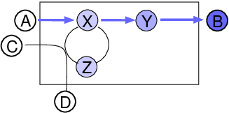
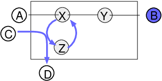
Our criteria for economical fluxes – the consistence with economic potentials and the absence of non-beneficial submodes – are closely related. In Figure 3, the flux profile in (a) is economical, as proven by the fact that economic potentials can increase along the flux. In contrast, to make the flux cycle in (b) economical, economic potentials would have to increase in a circle, which is logically impossible. Any flux profiles with this motif are uneconomical (for example, the one in (c)). A major advantage of the submode criterion is that it can be tested locally: we can discard an entire flux profile based on a local pattern, even without knowing the entire network!
| (a) Beneficial, economical fluxes | (b) Futile fluxes | (c) Beneficial, uneconomical fluxes |
|---|---|---|
 |
 |
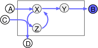 |
Figure 3 shows how economic potentials (of metabolites) are related to futile motifs (in flux profiles) and to economical enzyme usage. As a simple example model, we consider a kinetic model with a production objective and enzyme levels to be optimised. While the network structure allows for a cycle flux, this cycle is never active in enzyme-optimal states, no matter which rate laws or enzyme cost functions are assumed. The reason is simple: in optimal states, the cost of an active enzyme must be balanced by a positive benefit (or in the language of MCT): by a positive control on the metabolic objective function. In the flux cycle, this would not be possible. As we shall see below, this is in line with a general principle: if a flux profile is economical, it is possible to find economic potentials such that all fluxes run from lower to higher potentials. We can see this in Figure 3: in (a), the economic potentials increase along the flux profile, as required for an economical flux mode. In (b), potentials would have to increase in a cycle, which is logically impossible: flux profiles with this cycle are uneconomical, even the beneficial profile in (c). Mathematically, this criterion resembles an important thermodynamic criterion: fluxes must run from higher to lower chemical potentials (to dissipate energy in every reaction) [30]. Importantly, the two (economic and thermodynamic) constraints are logically independent. If metabolite C has a high chemical potential, the cycle in Figure 3 (c) will be thermodynamically feasible, but economically futile. Other flux profiles may also be beneficial, but thermodynamically impossible (under physiological concentrations), e.g. one that produces ATP from ADP and phosphate without any other conversions. Interestingly, FBA with flux minimisation, too, suppresses futile cycles. This is no coincidence: in models with a simple production objective, economic and thermodynamic feasibility becomes interdependent the two optimality principles – enzyme optimisation in kinetic models and flux minimisation in FBA – lead to the same flux solutions [24].

If flux profiles are depicted as points in flux space, the stationary flux profiles (nullvectors of the stoichiometric matrix ) form a linear subspace. By applying upper and lower flux bounds, we obtain the FBA flux polytope (see Figure 4). Thermodynamic constraints can be used to restrict the solutions: by excluding flux profiles containing thermodynamic cycles, we obtain a collection of convex polytopes, each representing a thermodynamically feasible flux pattern. Economic constraints have similar effects: non-beneficial flux patterns are excluded and flux profiles are restricted to feasible, i.e. economical segments of flux space (see Figure 4).
To understand the meaning of economic values and value production, let us step back and consider flux profiles that are solutions of an optimality problem, for example, a minimisation of flux or enzyme costs. The optimality conditions, as mathematical equations, contain fitness derivative and auxiliary variables called shadow values that arise from constraints [24]. For example, mass balance constraints in a model lead to optimality conditions that resemble our valure production equation while the shadow values in these equations play the role of economic potentials. Importantly, this holds for an entire class of (constraint-based or kinetics-based) problems: we always obtain the same balance equations! The economic potentials may vary, depending on kinetic constants, enzyme cost weights, or the flux cost function assumed, but we know that economic potentials exist and must be consistent with the fluxes. Conversely, if no compatible economic potentials exist for a given flux mode, this flux mode is uneconomical and cannot be the solution of an underlying optimality problem of this sort. Since the condition holds generally, we can use it in flux analysis, even without specifying the underlying problem in detail -- we just need to assume such a problem exists! This also means: if we postulate a value balance, economic potentials or enzyme investments may mean different things depending on the underlying optimality problem assumed66 6 A similar logic exists in thermodynamics: if we apply a sign constraint for fluxes, this constraint stems from an underlying variational problem for Gibbs free energy dissipation (details see below). If these flux constraints are fulfilled, we know that there must be a (thermodynamically consistent) kinetic model that realises our flux distribution (even if we don’t know this model in detail). Restrictions on (or estimates of) chemical potentials can make these unknown models more realistic.. Assuming that such an underlying optimality problem exists, we can search for economic potentials that correspond to plausible models (that is, models with plausible values of the kinetic constants and enzyme costs in line with protein data).
For the underlying optimality problems, we consider two possibilities (for other possibilities, see [24]). One possible interpretation is based on Flux Cost Minimisation (FCM) with a flux cost function . For plausibility reasons, flux costs should increase with the absolute flux, so . The shadow values in such models have been studied [31], compared to chemical potentials in thermodynamics [32], and interpreted as economic potentials [24]. The optimality condition of our FCM problem yields a value production balance equation of the form (2), with a flux burden and thus an investment (which, as we assumed, will be positive). Any flux profile that satisfies this balance equation will also be the solution of some FCM problem. In our second interpretation, we consider a different underlying optimality problem: a kinetic model with optimal enzyme levels and an increasing cost function . In this interpretation, the investment is actually and enzyme investment, defined as the enzyme point cost , which is positive (or zero for inactive reactions), see appendix . For example, with the size-weighted protein concentration (with protein sizes ) as our enzyme cost, a reaction has an investment . Below, will usually be called “enzyme investment”.
Which flux profiles allow cells to grow fast depends largely on the flux burdens, that is, the enzyme cost per reaction flux in every reaction. If Eqs (1) and (2) are based on an underlying FCM problem, the flux burdens are defined by the derivatives . If the flux cost function represents enzymatic costs, the burdens describe the enzyme cost per flux. In kinetic models, we define them differently: we consider enzymatic rate laws with enzyme efficiencies (called catalytic rates or apparent values) which depend on metabolite concentrations. Now flux burdens can be defined as , i.e. the enzyme investment per flux, or the enzyme price divided by the catalytic rate . In both modelling frameworks, economic potentials are the shadow values related to mass-balance constraints [24]. The term in brackets in Eq. (1), called flux value , is the sum of a flux gain and an indirect flux value . This second term represents benefits anywhere in the network to which our reaction contributes indirectly by supporting the steady state. Importantly, this term can be written as a difference of product and substrate values77 7 The symbol denotes the difference of a metabolite-specific variable along reaction . in the reaction. But how can we find the economic potentials? Flux gains and external economic potentials follow from our benefit function, but the internal potentials and enzyme investments remain to be found. In any case, the value production balance provides an important condition: since enzyme investments must be positive, fluxes and flux values must have the same signs: therefore, known flux directions constrain the economic potentials .
The economic potentials are not constant but vary with the metabolic state. Changing enzyme efficiencies will lead to changes in economic potentials: to see this, let us think about reaction kinetics and thermodynamics. First, according to Eq. (2), the economic potentials are closely related to the flux burdens . In kinetic models, with enzyme investments given by (with enzyme price ), a reaction flux burden reads
| (4) |
with the catalytic rate and enzyme slowness . At fixed enzyme prices , this means: as an enzyme becomes less efficient (e.g. at lower substrate levels or close to chemical equilibrium), more enzyme is needed to sustain the flux, and the flux burden increases. The higher investments (per flux) become embodied in downstream metabolites, increasing their economic potentials. How does thermodynamics come into play? The metabolite concentrations determine the chemical potentials (assuming activity coefficients of 1) and thermodynamic forces . The force in a reaction determines the ratio of microscopic one-way fluxes [33] and affects the net catalytic rate. Reversible rate laws can be written as88 8 Formula (5) holds for positive fluxes. The general formula reads where is the value in flux direction.
| (5) |
with a reversibility factor and a kinetic factor that depends on the rate law [34]. According to Eq. (5), the flux burden depends on reaction kinetics and thermodynamics:
| (6) |
By inserting this formula into Eq. (2), we can see how flux values and economic potentials depend on enzyme price , turnover rate , driving force , and kinetic efficiency factor . For a related question, the opportunity cost of one-way backward fluxes, see SI .
A metabolite’s economic potential describes the metabolites’ use value, i.e. its indirect effect on the metabolic objective. Together with the metabolite’s total consumption rate , it determines a value outflow . In optimal states, this outflow must be equal to a value inflow, descibring the nutrient and enzyme investments embodied in the metabolite. We can see this in Figure 5. In a linear pathway without flux gains, the enzyme investments accumulate along the flux, and the economic potentials increase by in each reaction. The initial substrate (with economic potential ) provides a substrate investment ; each enzyme provides an enzyme investment . Investments accumulate along the pathway, leading to an embodied investment in each metabolite , corresponding to an embodied value . Therefore, the economic potential of a metabolite X, , is given by the economic potential of the pathway substrate S, plus all enzyme investments between S and X, divided by the flux.
The “steps” in potential depend on the enzyme prices (e.g. their molecular mass) and inversely on enzyme efficiencies. Inefficient enzymes (e.g. enzymes with low values, substrate concentrations, or driving forces) are costly, and varying costs (per flux) entail varying embodied values in downstream metabolites! For instance, as the extracellular glucose level decreases, glucose transporters becomes less efficient and more transporter molecules are required to obtain a desired flux: this increases the embodied values of intracellular metabolites.
Aside from transporter and enzyme costs, embodied values may also reflect other terms in the balance equations: pathway substrates may add to embodied values downstream, while cofactors usage may add or absorb value within the pathway. Along the pathway, the embodied value increases, reflecting enzyme investments. If a reaction provides a direct benefit, this flux gain decreases the downstream embodied values, and if cofactor pairs are involved in reactions, their economic potentials are taken into account; due to such terms, economic potentials may sometimes decrease along the flux99 9 If potentials decrease along the flux, this may be due to non-enzymatic reactions or non-optimal enzyme levels..

3 Thermodynamic and economic constraints
Thermodynamic laws link the metabolic flux directions to chemical potentials via the thermodynamic driving forces (negative Gibbs free energies of reaction, in units of RT) [3, 4, 5]. These laws can be used to constrain fluxes, to exclude infeasible flux cycles [35, 36], and to constrain metabolite concentrations [6, 7, 8, 9, 10]. They also play a central role in the economy of the cell. All metabolic reactions must be exergonic, i.e. dissipate Gibbs free energy. A reaction’s energy dissipation rate (in units of ) is given by1010 10 If Gibbs free energy is dissipated in the form of heat and if other forms of energy can be neglected, is just the entropy (in units of ) production per volume and time. where is the thermodynamic driving force. In a physically feasible model, every active reaction must dissipate Gibbs free energy: the condition implies that (whenever ), or in short (“the flux profile is conformal to the force vector ”) [3, 4, 5, 6, 9, 10]. for our models, we obtain a sign relation between chemical potentials and fluxes1111 11 The inequality (7) follows from thermodynamic laws. In a well-mixed chemical solution at given pressure and temperature, each metabolite species (with mole number ) contributes an amount to the system’s total Gibbs free energy , and the contribution is given by , where (in kJ/mol) is called chemical potential. Reaction fluxes must dissipate Gibbs free energy. For a positive dissipation rate , a flux must have the same sign as the thermodynamic force , that is, it must lead from higher to lower chemical potentials. Without the condition in Eq. 7, we obtain the strong sign condition, requiring that non-zero forces evoke a flux in the same direction (see SI ).
| (7) |
which must hold for all active reactions. The chemical potentials are further related to metabolite concentrations: assuming constant activity coefficients, they are given by and therefore linear in . Thus, thermodynamically feasible flux mode requires a metabolite profile for which and have equal signs (in all active reactions).
In kinetic models with consistent reversible rate laws1212 12 “Consistent” means that the kinetic constants must satisfy Haldane relationships and the equilibrium constants satisfy Wegscheider conditions., energy dissipation and condition (7) are automatically satisfied. This holds for all rate laws of the form Eq. (5). In flux analysis, in contrast, the thermodynamic laws must be guaranteed by imposing condition (7) an extra constraint, which then allows us to detect and exclude infeasible flux modes. Given a flux profile , how can we see whether there exist consistent chemical potentials, satisfying condition (7)? At least it is easy to exclude this: in a closed loop of unimolecular reactions (without any other metabolites or cofactors being produced or consumed), a cycle flux cannot lead from higher to lower potentials everywhere. We can generalise this logic to more general types of cycle fluxes. A flux distribution dissipates energy at a total rate , with the vector of chemical potentials, the vector of chemical potential differences, and the vector of metabolite net rates (note that contains both internal and external metabolites). Cyclic flux profiles, without any net conversion of metabolites (), do not dissipate any Gibbs free energy and are thermodynamically infeasible (unless there is some extra “hidden” energy dissipation, e.g. through compounds ignored in the model). In general, this holds for any “flux cycles”, defined as nullvectors of the stoichiometric matrix (including internal and external metabolites). If a flux profile contains a cyclic submode (i.e. if and share all flux directions in their active reactions), the flux profile is infeasible. Hence, to obtain a feasible flux mode, such cycles must be excluded [30, 35, 37].
The formula assumes that our model actually describes all reactants. Sometimes, models are simplified by omitting some cofactors, protons, or water, and to keep the model correct, we use a formula with an extra force term that represents contributions of the neglected compounds1313 13 Note that this extra term can enable cycle fluxes that would otherwise be impossible. This makes sense: for example, if the extra term stands for an omitted cofactor pair, in reality these cofactors would be able to drive the cycle.. Similarly, a term in a model can always be replaced by the chemical potential of a virtual reaction product. This means that we can get rid of such terms, at least formally, by adding extra products to our reaction sum formulae.
When looking for possible cell states, we need to distinguish between what is thermodynamically possible in principle (allowing for arbitrary metabolite concentrations) and what is thermophysiologically possible (with metabolite concentrations within physiological bounds). For example, in theory any thermodynamic reaction can be reversed (by keeping the substrate concentration at zero or making the product concentration large enough). However, in real cells some reactions can never be reversed because the required concentration ratios will never exist in a living cell (for example, because of thermodynamic requirements in other reactions). To define thermophysiologically feasible driving forces and fluxes , we need to consider physiological concentration ranges (as, for example, in the MDF method [38].
Thermodynamic and economic constraints have very different justifications. While thermodynamic laws come from physics and must hold in any state of the cell, economic laws are based on the extra assumption of an optimal usage of enzyme. Given that thermodynamic and economic constraints are different in nature, why do they look so similar? Formally, both constraints can be derived from one variational principle, the principle of Flux Cost Minimisation (FCM) [18]. In FCM, a flux profile must be stationary and must minimise a cost function at a predefined benefit. Typically, flux cost functions represent enzyme investments or substrate consumption, while flux benefits represent biomass production or other production objectives. But we may use the same formalism to describe thermodynamics: treating negative energy dissipation as a flux cost, , FCM yields the thermodynamic flux condition Eq. (7) as an optimality condition (see SI ), with the negative chemical potentials as “economic potentials”.
The economic and thermodynamic constraints on fluxes, Eqs (3) and (7), in the version with direct (economic or thermodynamic) force terms1414 14 A direct force term in thermodynamics resembles – at least formally – the flux gain in the reaction balance equation. On the contrary, in the economic balance equations, we can always replace all flux gain terms by economic potentials of hypothetical metabolites, introduced just for this purpose: then we obtain the general simple relationship ., are mathematically similar. While thermodynamics requires a positive energy dissipation , value production Eq. (3) requires a positive flux benefit .
The similarity between these conditions leads to various other similarities between economic and thermodynamic constraints. In both cases, the flux directions depend on (chemical or economic) potential differences (plus, possibly, extra direct terms). Endergonic submodes in thermodynamics (which “absorb” Gibbs free energy) and wasteful submodes in enzyme economy (which “absorb” benefit) play a similar role. Also, in both cases, a condition for feasible flux profiles is that there exists a consistent choice of (chemical or economic) potentials. Likewise, uneconomical submodes can be found by considering futile flux variations: if a flux profile contains a futile submode it is uneconomical. And geometrically, when flux profiles are seen as points in flux space, economic constraints, just like thermodynamic constraints, exclude some segments in the solution space (see Figure 4).
Du eto their similar structure, formulae from thermodynamics can be transferred to metabolic economics. This concerns, for example, the role of cycles. Both types of conditions exclude flux profiles that would require potentials to increase in a circle [39, 36], which can be tested by searching for cyclic (in thermodynamics) or futile flux motifs (in metabolic economics). All flux profiles with such motifs can be excluded. To formally define these cycles, we first define infeasible submodes: in thermodynamics, infeasible submodes are elementary cyclic flux modes which represent thermodynamically infeasible flux variations. If a flux profile contains such a submode, the flux profile is thermodynamically infeasible. More details on thermodynamic and economic constraints can be found in SI .
Chemical and economic potentials describe different aspects of metabolism, but they are linked by the fluxes in optimal states. Fluxes must not only run from higher to lower chemical potentials, but also from lower to higher economic potentials. This effectively couples the two types of potentials. The thermodynamic condition and economic conditions imply that flux value and thermodynamic force must have opposite signs in all active reactions. By combining the two equations, we obtain a relation between flux values and thermodynamic forces:
| (8) |
Flux value and thermodynamic force must show the same ratio as enzyme investment and energy dissipation. So for example, if a reaction with predefined flux comes close to chemical equilibrium (), the flux burden becomes infinite and (in an optimal state) its flux value becomes infinite too.
Finally, there are models in which thermodynamic and economic constraints coincide: in models with a production objective (and without concentration bounds), cyclic flux modes are not only thermodynamically infeasible, but also futile. In this case, economic and thermodynamic constraints on fluxes are fully redundant (see SI ). This explains why FCM, originally designed to avoid futile and wasteful fluxes, can repress thermodynamic loops.
An important constraint on the economic potentials follows from molecule properties of the enzymes. In each reaction, the flux burden must be larger than where is the maximal catalytic rate of the enzyme1515 15 To derive the lower bound, we assume (without loss of generality) positive fluxes. In reactions with negative fluxes, would be negative and the inequality must be reversed. This also concerns all following inequalities. However, if we model a single metabolic state, this complication can be avoided by reorienting all reactions to have positive fluxes. and is the minimal price. By considering reaction thermodynamics (as in Eq. (6)), we obtain a stricter essential value that depends on the driving force . In enzyme-optimal states, flux value (value production per flux) and flux burden (enzyme investment per flux) must be equal in each active reaction. So for a positive flux, due to enzyme kinetics the flux value must exceed the essential flux value, which is given by
| (9) |
and therefore inversely proportional1616 16 The proof of Eq. (9) is simple: due to Eq. (6), with and , the flux burden has a lower bound . In cases where (full substrate saturation, no inhibition) and (large force), the flux burden hits this bound. Otherwise, if enzymes are inhibited or if substrate level is low, we obtain . Since flux burden and flux value must be balanced (Eq. (2)), we obtain the same bound for the flux value. to the force (see SI ). The resulting limits on flux values1717 17 Note that inequality (9) is an approximation of this bound. () and economic potentials () (see SI ) must hold for all active enzymatic reaction: if a flux value is below the essential value, the reaction must be shut off.
(a) Mass balance

(b) Thermodynamics

(c) Enzyme economy

The laws for metabolic fluxes and reaction thermodynamics resemble Kirchoff’s rules for electric circuits [40, 41]. Metabolic fluxes correspond to electric currents, and thermodynamic driving forces correspond to voltages. Kichhoff’s node rule (for currents) states that charge is conserved, so incoming and outgoing (steady) currents must cancel out for any region of an electric circuit (and in particular, for each node). The loop rule (for voltages) states that voltages, given by potential differences, must sum to zero over any closed loop. Similar rules exist in reaction thermodynamics: steady metabolic fluxes must satisfy mass conservation (like in the “node rule” for charge conservation), and thermodynamic driving forces, as potential differences, must sum to zero over a cycle (where “cycles” are defined more generally, as null space vectors of the total stoichiometric matrix ). Finally, like their electric counterparts, the thermodynamic forces determine the flux directions (sign constraint).
If we ask about the precise relation between forces and fluxes, or voltages and currents, we find some remarkable differences. In electric circuits, Ohm’s law states that a current is proportional to the voltage, with a constant current/voltage ratio (conductivity) and voltage/current ratio (resistance). Ohm’s law implies that nonzero voltages always cause currents (entailing a “strong sign constraint”). While Ohm’s law holds well for many conductors, it is just an empirical law and does not hold generally. In diodes, for example, the relationship is nonlinear and a threshold voltage must be exceeded to obtain a current. In reaction thermodynamics, the situation is even more complicated. The metabolic flux does not depend on the force directly, but on substrate and product concentration (via kinetic laws). Nevertheless, rate laws of the form exist as approximations. Near chemical equilibrium, a linear force-flux relationship is sometimes assumed, like in Ohm’s law. More generally, even without an exact force-flux formula, we may expect that “everything else being equal”, a higher force causes a higher flux. An example is provided by the factorised rate laws, where if the kinetic efficiency term is approximated to be constant. How are these force-flux relationships related to sign constraints? The weak sign constraint always holds due to basic thermodynamics. In addition, in a linear flux-force relationship, even the smallest force will lead to a flux (in line with the assumption of a strong sign constraint). But more generally, if enzymes can be completely inhibited allosterically, even a positive force will not always lead to a flux, so the strong sign constraint does not hold.
Now let’s compare this to value balance analysis. In fact, things are quite similar to thermodynamics: all three laws – node rule, loop rule, and rule for flux directions – hold, mutatis mutandis, for metabolic fluxes and “forces”, i.e. the flux values resulting from flux gains and economic potentials. What about sign constraints and “force-flux relationships”? While a positive flux value (or “economic force”) is necessary for a positive flux (hence the weak sign constraint always holds), the flux is not a function of the flux value. There is no Ohm’s law, and not even a nonlinear law like for diodes. However, like in thermodynamics, we may consider such dependencies metaphorically or as approximations, assuming that higher economic forces tend to go with higher fluxes. The “economic force” is typically given by an economic potential difference, but there may also be flux gains or values of cofactor pair that serve as an extra “voltage source” for the flux. An “economic flux-force relationship” is not based on a strict argument, but assuming a gradual dependence: starting from the facts that “without force, there is no flux” and “at some positive force, there will be a flux”, we claim that “the higher the force, the higher the flux”. In contrast to reaction thermodynamics, this relationship must for sure be nonlinear. We already learned that for a reaction to be active, the flux value must exceed some positive “essential” value given by enzyme molecule properties. Therefore, a force-flux relationship can only be a nonlinear one with a “threshold force”, like in electric diodes. This means that an economic “conductivity” or “resistance” cannot be defined, unless one defines it as the local derivative of the assumed force-flux relationship. It also means that the strong sign condition cannot hold.
4 Value balance analysis
In this section, we shall use economic and thermodynamic constraints together in a flux modelling framework called Value Balance Analysis (VBA). Similar to Energy Balance Analysis (EBA), VBA is not an optimality problem itself, but an algebraic framework to describe flux distributions that are stationary, thermodynamically feasible, and economical at the same time. We know that such flux distributions are exactly the potential solutions of some (unknown, underlying) metabolic optimality problems. Thus, our main aim is not to find a single solution, but rather sets of plausible solutions, which may stem from plausible underlying models (which, themselves, may be FBA-like, kinrtic, or part of hypothetical whole-cell models). This leaves space for sampling or for finding specific solutions by applying extra knowledge (in the form of constraints or heuristic selection criteria). In all these cases, VBA incorporates the idea of resource allocation by requiring that each feasible state (in VBA) must be an optimal state according to some underyling resource allocation problem!
Above we learned that flux directions are governed by thermodynamic and economic constraints. For flux analysis, it makes sense to use these constraints simultaneously. Consider a metabolic network with flux gain vector . To be economical, a flux profile must satisfy a value production balance (1) with suitable economic potentials , and since enzyme investments are positive, the fluxes and flux values must have equal signs. If all economic potentials were known, they would therefore determine the flux directions, and FBA could be used to find economical flux modes with these directions. However, a metabolic objective determines only the external economic potentials, while the internal potentials remain to be found. To do this, we consider a variant of FBA called Value Balance Analysis (VBA) in which fluxes, chemical potentials, and economic potentials appear as model variables. A VBA problem is defined by a metabolic network, a linear flux objective , and perhaps other data such as external potentials. For example, with biomass production as a single objective (), we obtain an economic potential for biomass and zero potentials of all other external compounds, and zero flux gains for all reactions. By splitting the effective flux gain into (see section 2), we obtain the external economic potentials and the flux gains as model parameters. The value production balance (1) provides a constraint besides the usual stationarity and thermodynamic constraints. Unlike the chemical potentials, which depend on metabolite concentrations1818 18 We use the common approximation , assuming constant activity coefficients., the economic potentials can be treated as separate variables (see SI ). Altogether, VBA describes fluxes and chemical and economic potentials (in vectors , and ) by the following three constraints (see Figure 6):
| (10) |
with thermodynamic driving forces and flux values . The symbol1919 19 Generally, (“ is conformal to ”) states that all non-zero components in have the same signs as the corresponding components in . denotes “equal signs in all active reactions”, and denotes “equal signs in all active enzymatic reactions”. External chemical and economic potentials (and maybe uptake and excretion rates) may be predefined, while all other variables need to be found.
The VBA conditions Eq. (10) state that our fluxes (at the chemical and economic potentials chosen) must be stationary, exergonic, and must produce positive value. All triples that satisfy these constraints are allowed. To further restrict the solutions, we may predefine some variables or constrain them to known or assumed physiological ranges. Together with a linear objective, this would yield mixed-integer linear programming (MILP) problems [42]. In contrast to the linear optimisation problems in classical FBA, such problems are typically non-convex and much harder to solve (see Figure 4). To keep the calculations simple, we do not use a MILP solver but choose our variables step by step. We first choose a pattern of feasible flux directions. To be (thermodynamically and economically) feasible, a flux pattern must allow for a stationary flux profile and for a choice of economic and chemical potentials (that it must be free of cyclic or non-beneficial submodes). Once we have such a flux pattern, we can easily determine all other model variables (stationary fluxes, chemical potentials, and economic potentials) by Linear Programming, separately for each type of variable. Thus, the only difficult step is to choose feasible flux signs: we may do this by choosing an (economically and thermodynamically) feasible flux mode, either by employing FCM or choosing a non-feasible flux profile and by eliminating all cyclic or non-beneficial motifs (see SI ). Given our flux pattern, feasible fluxes, chemical potentials, and economic potentials can be chosen independently. To choose a specific solution, we may use sampling or optimisation (with extra assumptions and usage of data).
How can we determine economic potentials in practice? In a state with known flux directions, Eq. (3) puts constraints on the potentials (see Eq. ()), just like thermodynamics laws put constraints on the chemical potentials (and thus on log-metabolite concentrations) [9]. If this is the only information we have, the economic potentials may be sampled, optimised, fitted to data, or chosen by heuristic rules within these constraints. The resulting enzyme investments can be computed from the value production balance. However, to realise these economic potentials by kinetic models [25], sampling our economic potentials at random may not be very wise: the resulting kinetic constants may be unrealistic. Anticipating this, we should choose realistic economic potentials from the start, for example by fitting them to measured enzyme investments. In fact, each set of economic potentials corresponds to an underlying kinetic models with specific kinetics and enzyme cost functions. If we are happy with arbitrary VBA solutions, we can freely choose the economic potentials within the given constraints. But if our aim is to construct kinetic models, all relevant data and constraints must be considered already when choosing the potentials. In particular, if we desire a realistic kinetic model, we need to use, at least, some good rules of thumb for integrating avilable data and constraints.
If the fluxes, metabolic objective, and enzyme investments in a network are known, it is easy to compute the economic potentials. In a linear pathway in an optimal state, they can be found like this: for each metabolite, we sum all upstream enzyme (and possibly substrate) investments; this yields the “embodied investment”. Then, by dividing by the metabolite’s production rate (in this case, the pathway flux), we obtain the metabolite’s embodied value. In an optimal state, this embodied value is equal to the use value (or “economic potential”). In networks with branches and cycles, this simple calculation method does not work because we cannot just sum the investments along a one path. Instead, we rely on the value production balance and the value balance , which define relationships between economic potentials , flux gains , fluxes , enzyme prices , enzyme levels , enzyme efficiencies , and flux burdens . Here is one possible calculation method. We use molecular weights as proxies for enzyme prices2020 20 Of course, also other measures for prices can be used, such as total synthesis rate, or ATP investment. (with a scaling factor to be determined later) and estimate the enzyme investments from proteomics data and enzyme prices. If fluxes or catalytic rates are known, we can estimate the flux burdens either by from enzyme prices, proteomics data, and fluxes, or directly by from and enzyme prices and catalytic rates. These estimates can further be corrected2121 21 The flux variation rule demands that the vector lies in the image space of , that is, in the nullspace of . Hence, to adjust a given vector , we can project onto this space (proof in [25]). to comply with the flux variation rule (see SI ), and be used to obtain the economic potential differences . From these potential differences, together with the known economic potentials of external metabolites and conserved moieties, we can compute the individual internal economic potentials.
If data are missing or uncertain, a “blind” choice of is not very practical, and we should use some extra information to obtain plausible values: for example, we consider how economic potentials are constrained (e.g. by flux directions) and then choose them to match measured enzyme investments (that is, enzyme investments reflecting proteomics data and assumed enzyme prices) as closely as possible. In practice, we can combine different measurement quantities, including flux and protein data, enzyme kinetic constants, and molecule sizes (as proxies for enzyme prices). If enough data are given and optimal states are assumed, the potential differences can be computed from our equations, and if data are missing, we replace them by plausible general assumptions. The aim is to choose economic variables that would also appear in realistic kinetic models. Some methods for computing economic potentials, relying on different data or plausible assumptions2222 22 Reasonable bounds on conversion values can be obtained from experimental data [43] (see SI )., are described in SI . We may assume, for example, that all reactions have equal enzyme investments (and therefore an equal value production ) or that they have equal flux burdens (and therefore equal flux values ), or that (uncertain) measurement data for some of these values are given. In all of these cases, we obtain simple “educated guess” formulae for the economic potentials and other economic variables (SI ).
| (a) Chemical potentials | (b) Economic potentials | (c) Enzyme point benefits |
|---|---|---|
 |
 |
 |
Given a metabolic model with known kinetics and a metabolic objective, we can determine an optimal state, which yields economical fluxes and economic potentials. Can we turn this around? That is, can any possible value structure – a set of compatible economical fluxes and economic potentials – be realised by some kinetic model in an enzyme-optimal state? We know that the answer is yes: such models can be constructed systematically. Figure 7 shows an example, a model of yeast central metabolism with ATP production as the benefit function. To reconstruct a kinetic model, we first determine a VBA-feasible (thermodynamically and economically feasible) flux profile (arrows) . We can do this by using linear FCM. Then, chemical and economical potentials are chosen by heuristic assumptions [25]. Data about enzyme levels, protein sizes, and catalytic constants can be used to estimate realistic economic potentials. Next, we search for kinetic models that realise our fluxes and economic potentials. There are many such models, and to construct one of them, we need to determine consistent economic loads and reaction elasticities satisfying the reaction-metabolite balance. From the elasticities, we can then reconstruct the kinetic constants [25]. This procedure leads to kinetically and economically plausible models that can be used for studying optimal metabolic behaviour, e.g. optimal enzyme adaptation to static or periodic external perturbations [45, 46].
Metabolic strategies arise from trade-offs between opposing objectives, e.g. achieving a high ATP or biomass production, at low metabolic fluxes [17]. Mathematically, trade-offs can be described by multi-objective problems: in a model with several flux objectives (e.g. production of different target compounds), each objective defines a pattern of flux gains , and each metabolite carries different economic potentials for the different objectives (or briefly a vectorial economic potential). By comparing the different potentials across the network, we can learn if the underlying objectives are compatible and where they clash (i.e. e. where there require different flux directions). How can trade-offs between the objectives be described? First, the individual sub objectives can be combined into a single objective function, for instance by taking a linear combination2323 23 Note that this also works for nonlinear combinations of objectives: in this case, the economic variables will be linear combinations with state dependent prefactors. : we obtain a single flux gain , and each metabolite has a single potential . Second, if subobjectives are uncertain or change rapidly, cells may adapt their enzyme levels to the average or expected objective (where subobjectives are weighted with probabilities or relative durations). Third, we may keep the subobjectives separate and search for Pareto-optimal states, i.e. states in which no subobjective can be improved without compromising the others [17]. Importantly, any Pareto-optimal state is also an extremal point of a single-objective problem, when the single objective is a convex mixture of the subobjectives (where the linear combination of objectives depends on the point on the Pareto front). This also means: any state on the Pareto front can be treated by VBA, assuming a combined single objective. Thus, in all three cases – combinations of objectives, uncertain objectives, and Pareto-optimal states – VBA can be applied, and the economic variables are given by linear combinations of the economic variables for the individual objectives.

If several objectives are given, it is unlikely that all of them can be optimised by a single metabolic state (i.e. by the same fluxes, metabolite concentrations and enzyme concentrations). However, if we do not require optimal flux profiles, but just enzyme-beneficial ones, a solution for several objectives may well exist. The situation resembles the case of a flux profile that simultaneously satisfies energetic and economic constraints (derived from “two objectives”, represented by chemical and economic potentials, and with right-hand sides of the balance equations representing energy dissipation and enzyme investment). In a multi-objective optimisation, each objective defines a set of economic potentials (a vector of economic potentials, as it were). A “lucky” flux profile that satisfies a value production balance for each type of potentials is extremely unlikely, but a variant of this can be used to model cell communities. Figure 8 shows an example, two cross-feeding cells which exchange compounds through a common flux profile. Each cell has its own objective (maximising its own biomass rate), defining two sets of economic potentials in the network containing both cells. To reach a maximal fitness, each cell must satisfy the value production balancesin its own enzymes, and with its own economic potentials: so as usually we obtain exactly one balance equation for each reaction.
In a cell community model, a Nash equilibrium is a state in which none of the cells would benefit from changing their fluxes and enzyme levels, given the behaviour of all other cells. All balance equations must be satisfied in cell A for the economic potentials of A, and in cell B for the economic potentials of B. To find such states, we may first run a multi-species VBA (in which each cell needs to satisfy its own balance equations, and with respect to its own benefit function; this is a necessary condition for a Nash equilibrium! The approach can be extended to cases with more than two species. Multi-species FBA models already exist, but these models typically employ a single “community objective”, that is, they presuppose symbiosis instead of explaining how symbiosis arises from cells pursuing their own benefit: there must be a Nash equilibrium in which each cell maximises its species-specific objective, given the other cell’s behaviour. VBA takes this into account. This approach – assuming “selfish” cell with different objectives, but sharing a common flux distribution, and searching for VBA solutions – describes not only cross-feeding, but also other Nash equilibrium states: for example, between a parasite and a host or between cells that are trapped in a “tragedy of the commons” dilemma, in which they consume nutrients fast, and inefficiently, just to gain a speed advantage over the other cells.
5 The principle of minimal fluxes
A feasible metabolic state, according to VBA, consists of an economically and thermodynamically feasible flux pattern and of fluxes , chemical potentials , and economic potentials compatible with this pattern. In fact, finding the flux pattern is the most difficult step: all other steps consist of linear problems (which can be satisfiability or optimisation problems, or variability analyis, depending on the puptpose of modelling) require. A feasile flux pattern can be obtained from a given feasible flux profile. In models with a production objective, we can compute such flux profiles by FBA with flux cost minimisation or molecular crowding . The principle of minimal fluxes [19], a heuristic rule for flux prediction, postulates that cells realise a given flux benefit at a minimal sum of (possibly weighted) absolute fluxes. Flux Cost Minimisation [18] generalises this principle to other flux cost functions, which can be linear (e.g. a weighted sum of fluxes in FBA) or nonlinear. Realistic flux cost functions (e.g. representing the cost of catalysing enzymes) follow from kinetic models [47, 15]: given a flux profile , we search for the enzyme and metabolite profiles that realise these fluxes at a minimal cost. This minimal cost, as a function of , yields an effective flux cost function.
Flux cost minimisation is closely related to VBA. With the value production balance as an optimality condition, it is no surprise that FCM predicts economical flux profiles2424 24 In FCM without flux bounds (e.g. upper bounds to restrict fluxes or lower bounds to enforce them), the logical connection to VBA is easy to see. Flux constraints in an FCM problem lead to extra shadow values that act as effective flux gains and appear in the flux benefit function in VBA and in the economic reaction balance. SIEHE ENDE SECTION 5 (“principle of min fluxes”)! In fact, different optimality problems – Flux Cost Minimisation (including FBA with weighted flux minimisation) and enzyme optimisation in kinetic models – yield the same sets of solutions, which are also the solutions of VBA (see Figure 9). In each method, the solutions depend on model parameters (e.g. flux cost weights in linear FCM or enzyme cost functions in kinetic models), but the range of possible solutions (obtained by screening all model parameters) is always the same. An economical flux mode (with some flux benefit function ) is the solution of a linear FCM (with the right flux cost weights), of a nonlinear FCM (with the right flux cost function), and of an enzyme optimisation (with the right enzymatic rate laws and enzyme cost function): all these methods predict econonomical flux profiles, and their solutions also can also be described by VBA with the right potentials and enzyme investments.

Why do all these optimality problems predict economical flux modes? The reason is that all of them share an optimality condition of the same form, a value production balance. In VBA, this value production balance is imposed as a dogma. In all cases, value production balance arises from mass-balance constraints. In optimality problems, these constraints give rise to shadow values. There is another explanation for the strange agreement between modelling frameworks. Any enzyme-optimal kinetic model can be converted into a linear FCM problem with the same solution: given an enzyme-optimal state, we constrain our model to the optimal metabolite concentrations; fluxes and enzyme levels are now proportional, and enzyme cost can be minimised by solving a linear FCM problem! On the contrary, given the solution of a linear FCM problem (with flux prices and solution ) and a kinetic model that can realise the same fluxes (with a enzyme profile ), we can adjust the enzyme prices such that , thus putting the kinetic model into an enzyme-balanced state. On a more theoretical level, a kinetic model (with an optimal state ) can always be replaced by an FCM problem (with an optimal flux profile ), where the given benefit function stems directly from the kinetic model and the flux cost function is the enzymatic flux cost function for the kinetic model, subject to . The FCM problem recovers the kinetic problem, but restricted to a submanifold in state space (which contains the optimal point). This shows that FCM is a good starting point for a systematic kinetic model construction as described above (also called “layered modelling”).
We already saw that economical, thermodynamically feasible flux profiles can be easily found by linear FCM. By varying the flux cost weights, any economical flux profile can be obtained, and by sampling cost weights at random, we can construct an ensemble of economical flux profiles, with given flux directions. Each of these profiles yields a feasible flux pattern, and for each of these patterns, other economical flux modes can be found by classical FBA or by flux sampling. As a side results, the FBA solutions yield shadow prices for mass-balance constraints, which can be seen as economic potentials. All the resulting solutions satisfy the constraints of VBA and can be realised by kinetic models in enzyme-economical states.
6 Futile cycles
We can now address some questions raised in the introduction. Are there flux profiles that entail a waste of enzyme in any kinetic model? And can we recognise them by typical “futile patterns”? A good example is futile cycles that degrade valuable compounds without an obvious benefit. Figure 10 shows an example, a cycle formed by two enzymes in upper glycolysis. Phosphofructokinase (PFK) transfers a phosphate group from ATP to fructose 6-phosphate (F6P), converting it into fructose 1,6-bisphosphate (FBP). Fructose bisphosphatase (FBPase) catalyses the backward reaction, but instead of generating ATP it releases phosphate. Together, the two enzymes can drive a cycle that splits ATP into ADP and phosphate and releases heat. To save valuable ATP, cells can interrupt the cycle by inhibiting or repressing at least one of the enzymes. In FBA, this cycle is often excluded manually by applying a constraint. But can we justify this more generally, based on a principle of optimal enzyme usage?
In VBA, instead of spotting futile cycles intuitively, the notion of “futile cycles” is given a precise meaning. Futile or wasteful flux motifs are hallmarks of uneconomical enzyme usage. As we learned above, economical flux distributions must be free of futile or wasteful motifs! In a flux profile , a futile motif is a set of active reactions that can support, by itself, a futile flux profile with the same flux directions as in . Similarly, a wasteful motif is a reaction subset that can support, by itself, a wasteful flux profile (with the same flux directions as in ). Futile submodes may look like cycles, but may also arise in linear pathways without a valuable product. Unlike existing verbal or topological definitions of futile cycles [48], this algebraic definition allows for clear statements about optimal metabolic states: futile or wasteful motifs make a flux mode uneconomical, i.e. incompatible with a feasible choice of economic potentials or optimal enzyme profiles in kinetic models. Moreover, a futile motif tells us in which reactions resources are wasted.

Let us come back to the PFK-FBPase cycle. To see why cycle fluxes should be repressed, we analyse all feasible and all infeasible submodes, considering thermodynamic and economic constraints (Figure 10). The choice between glycolysis and gluconeogenesis (without cycle flux) depends on the economic potentials. Generally, a high economic potential of FBP favours glycolysis, while a low economic potential favors gluconeogenesis: however, there can be economic potentials for which both flux are uneconomical: if both and (which implies that (note that water has been omitted for simplicity.), we find that the cycle flux is economically infeasible in forward direction and thermodynamically infeasible in reverse. If ATP (plus water) has a higher value than ADP (plus phosphate) and if there is not direct flux beneficial (e.g. heat production being beneficial), the PFK-FBPase cycle in forward direction is not beneficial, and flux profiles with this cycle are uneconomical. We can tell this just from the economic potentials, which represent fitness demands in the entire cell: given these potentials, it does not matter whether ATP, ADP, and phosphate are modelled as external or internal metabolites, and not even whether the rest of the network is known. Running the cycle in reverse (Figure 10c, left) would produce ATP, but it would require a drop in chemical potential between FBP and F6P, implying unphysiological concentrations. Since both cycle cirections are infeasible, to avoid an uneconomical flux the cell needs to interrupt the cycle by repressing an enzyme. This is no surprise, but now we have found a way to formally derive this very generally from metabolic models. Of course, this does not exclude futile cycles in reality. Here we just say that these cycles would contradict certain simple optimality principles, and how this can be checked.
If all enzymes in a cell were expressed simultaneously, this could easily lead to futile or wasteful cycles. To disrupt futile cycles, cells need to express enzymes selectively, i.e. repress some enzymes. How can we describe this in models? To disrupt futile cycles, we first need to find all such cycles in a given flux distribution. To see if a given flux distribution is economical, we may search for compatible economic potentials (by solving a linear programming problem): if no solution exists, the flux distribution is uneconomical. However, this does not tell us where the problem is localised, i.e. what reactions we need to suppress to make the flux profile economical. In theory, we can detect and remove futile cycles by enumerating and subtracting all non-beneficial submodes, but in practice this would be impossible: any given pair of flux distributions can be linearly combined to yield a futile flux profile! Luckily, we only need to consider elementary futile test modes2525 25 A futile submode is elementary if it does not contain any smaller futile submodes [49, 5]. Elementary wasteful modes are defined similarly., which can still be enumerated in medium-sized networks. The yeast metabolic model in Figure 11 contains 303894 elementary futile modes (calculated by efmtool [50, 51]). Many of these modes are large (the average size is 32 active reactions). By comparing a flux profile to each of these modes, we can find its futile motifs, and thus the reactions that make it uneconomical.
If a flux profile contains known futile motifs, we can use them to correct the fluxes. By using a flux motif as a flux variation , we can substract it from the flux profile and interrupt the cycle. In the corrected flux profile , the prefactor is chosen to cancel one reaction flux in the submode, but without reverting the flux directions, which leaves it thermodynamically feasible. By repeating this procedure, any infeasibile submodes can be removed (see SI ). An example is shown in Figure 3. To remove the cycle from flux mode (c), we subtract from it the elementary cycle from Figure (b) and obtain the flux profile shown in (a). Thermodynamically infeasible modes can be removed similarly and along with the futile modes [35].
| (a) Futile PFK/FBPase cycle | (b) Number of futile submodes per reaction |
|---|---|
 |
 |
To ensure economical flux profiles, cells need to suppress non-beneficial, thermodynamically feasible submodes. They can do this by repressing one enzyme in each of these submodes2626 26 If enzymes are repressed transcriptionally, protein production costs are saved. Posttranscriptional inhibition does not save enzyme costs, but can prevent a waste of metabolites. Therefore, futile submodes should be disrupted transcriptionally, while wasteful submodes may be disrupted by posttranscriptional inhibition.. If an enzyme appears in multiple non-beneficial submodes, this makes it a plausible target for regulation. By this criterion, PFK and FBPase rank among the top regulation targets in the yeast model in Figure 11. But how can the switch between glycolysis and gluconeogenesis be realised biochemically? If both PFK and FBPase expression were dependent on a common regulation parameter, there might be a parameter range in which both enzymes are partially active, causing a futile cycle. To prevent this, the two enzymes should rather be controlled by a bistable switch (implemented, for instance, by a positive feedback in transcriptional or post-transcriptional regulation).
We saw that cells can block non-beneficial submodes by enzyme repression. But what can we learn from VBA about network structures in general? Obviously, network structures that enforce non-beneficial submodes should not even exist: metabolic networks should be such that (thermodynamically feasible, but) non-beneficial submodes should either be avoided (by suitable network structures) or be subject to regulation. According to VBA, non-beneficial flux modes -- such as potential futile cycles or unnecessary biosynthesis pathways -- will waste economic value. Unless they are thermodynamically infeasible (and therefore, be excluded by physics), they should be selected against2727 27 For the sake of the argument, we consider a non-beneficial flux mode that actually provides no benefit at all, under any reasonable constraints or side objectives.. What will the resulting networks look like? First, each reaction or pathway should contribute to at least one beneficial flux mode. Second, non-beneficial submodes should contain two repressible enzymes2828 28 In a non-beneficial submode with only one repressible enzyme, this enzyme would always be repressed and would not be conserved in evolution.: the PFK-FBPase system is an example. These rules can also be used as sanity checks in automatic network construction.
It seems like futile (or wasteful) cycles are relatively common in cells. During autophagy, for example, proteins are degraded and produced at the same time. Kinase-phosphatase cycles in signaling systems constantly burn ATP. How can such cycles be reconciled with our theory? It may be that some cell processer are simply not optimal (in fact, there is no reason to believe that cells work precisely optimally in reality). But maybe some of this depends on what objectives we attribute to a cell. If a cycle looks futile, it may still have beneficial side effects or may be enforced by constraints. For example, flux cycles may enable cells to rapidly change their fluxes or to escape from unfavourable metabolic states [52]. A “futile” consumption of ATP may improve information processing (in signaling systems), increase precision in DNA replication, or speed up responses in gene expression [53]. Trehalose cycling, a “futile” cycle in yeast, can prevent a breakdown of metabolic fluxes caused by the “turbo design” of glycolysis [52]. Other cycle fluxes may be beneficial due to the ensuing heat production: in a compost pile, for example, higher temperatures increase the enzymatic rates and therefore the growth of bacteria. If we include them in a model as side benefits, this leads to extra terms in the economical balance equation, and a “non-beneficial” cycle may become beneficial. A particular reason for apparently futile cycles are non-enzymatic reactions: if a degradation reaction cannot be suppressed, cells need to reproduce the degraded metabolites to keep them at a desired concentration. In this case, the economic potentials will show an unusual pattern with a drop in the degradation reaction. Normally, such a drop would indicate an uneconomical flux mode, but if a non-enzymatic reaction (or in a dilution flux) is involved, a certain value loss cannot be avoided, not even in optimal states. In metabolic value theory, non-enzymatic reactions can be taken into account and such flux profiles are correctly classified as economical [25].
7 The choice between metabolic strategies
Once we we can which flux profiles are economical, we may ask about choices2929 29 “Choosing” is of course used metaphorically, similar to “machine learning”, “automatic reasoning”, or “evolutionary games” in other contexts. In all these cases, we hypothetically replace a physical system (a cell, an organism, or a computer) by a conscious being and ask how this being should behave, if it were in the place of our system and had to perform the same task. between metabolic pathways and how these choices depend on enzyme efficiencies (and thus, on metabolite concentrations). Cells may choose between metabolic strategies (e.g. between different carbon sources or between different excretion products) by expressing different sets of enzymes. Which choices are best, and how does this on details of enzyme kinetics? If an enzyme is inhibited or knocked down, should other enzymes in the pathway be upregulated (to compensate the decrease in activity) or should the entire pathway be switched off (and the flux be rerouted to other pathways)? Finally, should cells produce ATP by high-yield or low-yield pathways (see Figure 13)? Eventually, all these criteria are related to the pathway’s effective catalytic rate, i.e. the enzyme amount per pathway flux. More generally, evolution may favour pathways with high enzyme productivity (e.g. the target flux per enzyme investment) or with high substrate productivity (target flux per substrate consumption). In some cases, the two criteria coincide: a low yield (substrate productivity) may imply a low enzyme productivity (e.g. due to the larger import fluxes, and therefore higher enzyme investments). In other cases, a low yield may cause a higher enzyme productivity (because more energy is dissipated, allowing enzymes to work more efficiently). VBA does not only consider absolute catalytic rates but provides a new perspective based on values (i.e. marginal cost and benefit), relates economic potentials to enzyme investments and fluxes, and explains the choice of fluxes depends on prior protein investments “embodied” in the metabolites.
In VBA, flux profiles must be compatible with patterns of economic potentials: if the economic potentials and flux gains are known, they directly determine the flux directions. In turn, known flux directions put constraints on the economic potentials. But all this is also related to enzyme kinetics. Known enzyme prices , enzyme levels , and fluxes determine the potential differences : in reactions without direct flux gains, the potential differences are proportional to the enzyme levels (with as a prefactor) and to the inverse enzyme efficiencies (or “enzyme slowness”) (with the enzyme price as a prefactor). Furthermore, since enzyme efficiencies depend on metabolite concentrations, varying concentrations can make pathways either economical or uneconomical. To see how all this shapes metabolic states, we need only two equations: the value production balance (for reactions and pathways) and the relation between flux burden, kinetics, and enzyme price (which defines a minimum flux value). Using the equations, we now ask whether a given pathway should be used at all, which out of several alternative pathways should be used, and whether fluxes through alternative pathways should be combined.
If we split a metabolic network into pathways3030 30 For the present purpose, the term “metabolic pathway” is used in a general, rather formal way: it may refer to any set of reactions, a single reaction, or the entire network., the cofactors and precursors on their boundaries serve as “interfaces” between the pathways [54]. In metabolic economics, these boundary (or ‘‘connecting’’) metabolites play an important role. First, their economic potentials and production rates (by a given pathway) determine the total enzyme investment inside the pathway3131 31 The enzyme investment in a pathway is equal to the value production at the pathway boundaries, which depends on boundary potentials and fluxes. This equality resembles Gauss’ theorem in vector analysis, which equates the flow across a closed surface to the sum of sources of this flow in the enclosed region [25, 55]. In electrostatics, it describes the relation between charges and fields. Instead of treating enzyme investments as “sources” of value, we may count enzyme investments as a “value consumption” or value flowing in from the rest of the cell, and matching metabolic value production. Described in this way, the overall value flow across the boundary of a pathway must vanish, and we obtain a conservation relation for value (in optimal states) without sources and sinks, but with enzyme investments counted as inflowing value! The analogy suggests that metabolic values can be described by a conserved flow [56]. . Second, under some heuristic assumptions, the economic potentials and rates on the pathway boundary determine all economic potentials and enzyme investments inside the pathway. Third, when modelling a single pathway, all relevant information about the outside system is encoded in the economic potentials on the pathway boundary. This facilitates modular modelling: if a cell state changes, and if we know the changes of variables in the connecting metabolites, this sufficies to understand the economic adaptations inside each pathway, independently of the rest of the network.
To quantify enzyme investments in pathways, we first note that a pathway, just like a single reaction, satisfies a value production balance. For a pathway (or for that matter, any set of enzymatic reactions), we can sum Eq. (1) over the reactions to obtain the pathway balance
| (11) |
Internal metabolites must be mass-balanced, so their value production and consumption cancel out and the first term depends only on value production on the pathway boundary3232 32 Let us see this in detail. Pathway metabolites that participate in reactions outside the pathway are called boundary metabolites. They are produced or consumed by the pathway. Pathway intermediates, in contrast, are mass-balanced in steady state, so their value production and consumption cancels out. Therefore the first term in Eq. (11), describing value production, depends only on the economic potentials and production rates of boundary metabolites. Therefore, value production can be split into terms for internal metabolites, pathway substrates, and pathway products (12) where the first term vanishes due to mass balance: the production and consumption of internal metabolites cancels out, and so does the associated value production and value consumption.. The pathway’s total enzyme investment, on the right of the pathway value production balance Eq. (11), is given by
| (13) |
Treating the pathway as a single effective reaction (with a rate describing the pathway flux), this investment can be written as , with the total enzyme concentration and the (state-dependent) enzyme price . Eqs (12) and (13) apply not only to “dedicated” pathways, but to any part of a network. Applied to the network as a whole, they state that total enzyme investment and total metabolic benefit (e.g. of biomass production) in the network must be equal.
As mentioned before, each enzymatic reaction (with a given direction), has an essential flux burden defined by enzyme molecule properties. Via the value/price balance (2) , this burden defines a lower bound on the possible flux values. Below this value, the balance cannot be satisfied and the reaction must be inactive. Eq. (12) implies a similar condition for any flux mode in a network (and for any pathway defined by a localised flux mode). For example, in a linear pathway a positive flux requires that : the potential difference (left) must exceed the essential flux burden (right) of the pathway.
How does the choice between alternative pathways – for example, importing a compound or producing it in the cell – depend on model parameters such as the composition of the growth medium [18]? In VBA, which fluxes are possible depends on the economic potentials of pathway substrates and products: the pathway’s flux burden (which depends on the catalytic rate)3333 33 Metabolic fluxes and enzyme levels in cells are not simply proportional. Instead, when enzyme levels are changing, this leads to a new steady state with new metabolite concentrations, enzyme efficiencies, and steady-state fluxes. The relation between enzyme levels and steady-state fluxes is complicated and depends on many model details including rate laws and small-molecule regulation of enzymes. The resulting changes in enzyme efficiencies also cause changes in flux burdens. must match the external potential difference. If a pathway is active (i.e. if it satisfies the balance condition), then costlier alternative pathways (with a higher flux burden) cannot satisfy the same condition: instead they are uneconomical and must be suppressed. We can see this for a single reaction: isoenzymes, which catalyse the same reaction, have the same flux value . This means: in an enzyme-optimal state, isoenzymes cannot be active simultaneously unless their flux burdens are exactly equal. In a given model, this will not happen by chance. Thus, to minimise its enzyme investment, a cell should use only the cheapest isoenzyme, and in each moment there is probably only one. FCM (with randomly chosen cost weights) also predicts this, but without giving a general explanation. VBA provides a local criterion for pathways that should be suppressed: a cost-efficient enzyme “clamps” the flux value by equating it to a low flux burden, so costlier isoenzymes must be inactive. When the enzyme is inhibited or knocked out, the flux value can increase and another isoenzyme may be used. This logic holds also for isopathways, i.e. alternative pathways with the same substrate/product stoichiometry (or with the same single production objective, e.t. ATP production).
How can we understand ecnomical fluxes, economic potentials, and enzyme investments in larger networks? If we split a network into separate pathways, the economic potentials of the connecting metabolites can tell us which pathways are economical under which conditions. In particular, they tell us which pathway fluxes are beneficial (i.e. able to balance a positive flux burden) and whether the flux values are above the essential flux burdens (otherwise pathways must be inactive). Second, given the fluxes, known boundary potentials determine the total enzyme investment in each pathway (11). Third, by employing simple heuristic assumptions (e.g. uniform enzyme investments, see SI ) we may estimate the economic potentials inside the pathways from potentials on the pathway boundaries. If the boundary potentials are changing (e.g. the potentials of key precursors or cofactors), the internal economic potentials in each pathway will change as well3434 34 Under simple heuristic assumptions (e.g. assuming that all unknown enzyme prices should be identical), an increase of all economomic potentials on a pathway boundary increases the potentials inside the pathway (SI ). In contrast, if the potential difference between pathway substrates and products increases, the extra potential difference will be distributed along the pathway. This leads to higher flux values within the pathway, and in optimal states, higher flux burdens. If the pathway flux remains constant, this entails a higher enzyme investment, and according to Eq. (6), lower enzyme efficiencies., and it may be profitable to switch different pathways on or off.
8 High-yield and low-yield pathways
In an environment that favours fast growth, cells are expected to maximise enzyme productivity (biomass production per enzyme investment), a proxy for growth rate [57]. In an environment with limited substrate, cells are expected to maximise cell yield (biomass production per uptake rate). Depending on enzyme investments, kinetics, and external conditions, high growth rates may be achieved by either high-yield or low-yield flux modes [15]. This concerns, for example, fermentation or respiration or variants of glycolysis with different ATP/substrate yield [58]. How can we predict such choices by models? Different flux prediction methods favour different objectives. Classical FBA, with bounds on individual fluxes, predicts substrate-efficient behaviour (high yield), which may not be enzyme-efficient. In contrast, FBA with flux minimisation [19] or molecular crowding [59] are made to predict enzyme-efficient flux modes, which may or may not be substrate-efficient.

Let us consider an example, the usage of overflow. In aerobic conditions, cells typically respire, but they may further increase their glycolytic flux by adding extre fermentation. In experiments, the choice between respiration and (extra) fermentation depends on the extracellular glucose concentration, suggesting that glucose concentration determines the relative advantage of the two strategies. In FCM (including FBA with a minimal sum of fluxes, EFCM [18] or satFBA [60]) different strategies are scored by their enzyme costs at a given production rate, e.g. ATP production. Given an enzyme cost function, each flux profile will have a (minimal possible) enzyme cost which depends on kinetic constants and extracellular concentrations. Such enzymatic flux costs can be defined for single reactions, pathways, or entire flux distributions. Let us see an example (Fig. 13), where we compare (low-yield) fermentation to (high-yield) respiration at a given ATP production flux. Fermentation needs a higher glucose influx and therefore uses a higher amount of glucose transporters and glycolytic enzymes (at a given glucose concentration). Respiration, in contrast, uses the costly TCA cycle and oxidative phosphorylation. At high glucose levels, fermentation will be relatively cheap. At low glucose levels, the cost of transporters and glycolytic enzymes increases: both strategies become costlier, but since fermentation relies on these enzymes more strongly, at some point it will lose its advantage: (high-yield) respiration becomes comparably cheaper and allows for faster growth. This effect has been compared to Giffen behaviour in economics [61].
If external metabolite consumption is “costly” (i.e. if uptake is directly penalised by the metabolic objective), metabolite uptake should be kept low, and the metabolite should be used efficiently, i.e. with a high yield. The same holds for a metabolite that is taken up via a costly transporter: also in this case, a high-yield strategy will be preferred. This means: what exactly makes the uptake costly (metabolite usage, investments in transporter, or anything else) does not matter for the choice of the downstream metabolic strategy, it is only the cost that counts. In VBA, this logic holds not only to extracellular substrates, but to any metabolites: in a reaction A B, if the concentration of A is low, a large amount of enzyme is needed; this makes B effectively costly, and in the rest of the system, B should be used economically! Let us describe this in the language of VBA. The economic potentials in optimal states arise from embodied investments, e.g. usage of extracellular substrates, transporters, and enzymes needed to produce a metabolite. Exporting a metabolite with a positive economic potential (i.e. converting it into a worthless extracellular metabolite) would be uneconomical; instead, this metabolite should be converted into a valuable product (even if this requires additional enzyme investments). This means: in enzyme-optimal states, high investment along a pathway, leading to valuable intermediates, also require a high yield3535 35 Metabolites that embody investments can be compared to backgammon stones which become more valuable the more they advance. The more points have been “invested” in a stone, the less a player would typically sacrifice this stone. . This explains why the choice of metabolic strategies depends on extracellular concentrations.

Economical states may either show a balance between high value production and high enzyme investment (high-yield strategy), or between low value production and low enzyme investment (low-yield strategy). Which type of balance we find will depend on external concentrations, kinetic constants, or enzyme prices. Figure 13 shows an example. In central metabolism, glucose is converted into an intermediate C (for example pyruvate, lactate, or ethanol) which can either be exported (overflow with a low ATP yield) or further oxidised (by respiration, with a high ATP yield). Classical FBA favours respiration because of its higher yield. In VBA, either of the strategies can be economical, depending on their ATP/enzyme productivity. In kinetic models, the ATP production per enzyme investment is hard to determin because it depends on model parameters. However, there is an interesting rule of thumb: how a metabolite should be used depends on the enzyme or substrate values embodied in the metabolite. We can see this in Fig. 12. If external glucose levels are low, glucose transporters are inefficient, and many transporter molecules are needed to achieve a desired influx. This transporter investment is embodied in downstream metabolites, leading to high economic potentials, and the cell cannot waste these costly metabolites in a low-yield strategy. In contrast, high glucose levels make the metabolite’s embodied value decreases, and as its economic potential becomes negative, a low-yield overflow strategy may become economical. We can also see this more formally. In the respiration strategy, metabolite C has a positive economic potential, so exporting it (i.e. converting it into a less valuable metabolite E) would be uneconomical. Instead, additional enzyme is invested in respiration to produce more of the valuable A. Figure 13 (c) shows the conditions for fermentation. Due to lower investments (e.g. higher external glucose levels, and thus lower (flux-specific) transporter demands) C has a negative economic potential. So a costly export reaction can satisfy the reaction balance equation. When this model was previously analysed by FBA with flux minimisation , the optimal fluxes were found to depend on the total burden (enzyme investment per flux) of respiration or export flux. Now we can see, additionally, a dependence on embodied values, i.e. at what cost a metabolite has been produced, given the economic value of external glucose and the cost of transporter and glycolytic enzymes. The explanation is in line with previous arguments about rate/yield trade-offs based on thermodynamic forces and substrate availability (see SI ).
If a cell “chooses” between alternative pathways, we can describe this as a choice between flux modes in which different pathways are active (for example, elementary flux modes or extreme rays). But what about mixed metabolic strategies (i.e. linear superpositions of such modes)? For example, if several carbon sources are available, should a cell consume them one at a time (investing in a single transporter only), or simultaneously (distributing its investments over several transporters)? Similar questions concern alternative transporters with different affinities, isoenzymes, the choice between fermentation or respiration, or variants of glycolysis with different yield [58]. In all these cases, we can ask: should alternative reactions or pathways (with different kinetics and costs) be used separately or in combination? In VBA, combined flux profiles can be economical, but in th eunderlying optimality problems they are usually not enzyme-optimal unless they are enforced by flux bounds ( see SI ). In kinetic models (with realistic enzyme parameters), alternative enzymes or pathways show different cost efficiencies, and the most cost-efficient flux mode should be preferred (see SI ). FCM makes the same prediction: since realistic flux cost functions are concave in flux space, optimal flux modes are vertices of the flux polytope, and mixed flux strategies will not be optimal [15, 18]. However, these arguments hold only theoretically. In reality, cells may face limitations (e.g. limited membrane space) or a need for preventive measures that favour mixed strategies rather than specialising on one single task. 3636 36 In flux sampling, this is a question of practical concern: should we sample “pure” flux profiles (e.g. EFMs) or linear combinations of flux profiles? If we assume that cells realise enzyme-optimal states, we should in fact sample pure profiles , i.e. vertices of the VBA polytope. But if we mistrust our optimality assumption or look for economical (but not necessarily optimal) strategies, we may sample combined strategies from the entire polytope (see Figure 4)..
9 Discussion
Optimality problems in kinetic models lead to a value structure, a pattern of economic potentials that represent the network-wide (indirect) benefit of each metabolite. Understanding this value structure can help us obtain plausible flux profiles in FBA: by requiring that flux profiles must be compatible with a feasible value structure, we know that they are realisable by kinetic models in enzyme-optimal states. Flux profiles with a positive benefit are called beneficial. If such a flux profile satisfies the flux variation rule with positive enzyme investments , it is called economical. Such flux profiles are in principle able to produce value in every reaction. This property depends only on flux signs, that is, active reactions and flux directions. Like thermodynamic constraints, economical flux patterns can be imposed manually or by evoking general laws. First, metabolic value theory provides some useful theoretical concepts: the flux variation rule is an algebraic condition for economical fluxes, independent of enzyme kinetics [25]. A second, equivalent criterion states that economical flux profiles require the existence of compatible economic potentials, just like thermodynamically feasible fluxes require the existence of compatible chemical potentials. Third, just like feasible chemical potentials exclude flux cycles and ensure thermodynamically feasible fluxes, feasible economic potentials exclude non-beneficial flux motifs and ensure economically feasible fluxes. Non-beneficial flux motifs are flux patters that can never – under no conditions – contribute metabolic benefit and that always imply a waste of resources.
To achieve fast (or sustainable) growth, cells need to run their metabolism efficiently, i.e. with a high metabolic benefit at a low enzyme cost. Metabolic value theory provides concepts to understand this [25]. In the optimal state, value production must match enzyme investments3737 37 Biomass/enzyme productivity (biomass production rate per total metabolic enzyme) can be converted into cell growth rates by a simple function related to bacterial growth laws [15]., a principle that shapes metabolic states. First, flux profiles need to be economical to appear in optimal states. Whether a flux profile is economical depends only on flux directions and active reactions, and not the quantitative fluxes. Second, the economic balance equation quantifies optimal enzyme investments. It requires economical fluxes, resembles the thermodynamic flux constraint, and is used in VBA as a constraint for flux prediction. VBA does not describe the underlying problem directly and we don’t even need to know it precisely – we just assume that it exists, and make our FBA compatible with it by imposing the balance equation. It applies three basic principles -- fluxes must be stationary, must dissipate Gibbs free energy, and must produce metabolic value to balance to balance the enzyme investments3838 38 Ignoring thermodynamic laws may lead to paradoxical results [25]. Consider a linear pathway: if a reaction is fully forward-driven (infinite thermodynamic force), the downstream enzymes have no flux control. If these enzymes are downregulated, their substrate levels increase, but the flux does not change. Paradoxically, these enzymes provide no point benefit even though they are needed for catalysing the flux. In metabolic value theory, this paradox can be avoided by prohibiting fully irreversible rate laws [62]. . It provides a physically, biochemically, and physiologically meaningful theory of metabolic fluxes, provides a solid definition of futile cycles, and explains patterns in proteomes.
In VBA, the economic potentials play a central role. If a small extra influx of a metabolite (as a “gift”) allows for an increase of the metabolic benefit, the ratio is called the metabolite’s economic potential. Even if the objective scores only a single flux, this flux still relies on the entire metabolic state. This gives every metabolite a value: the metabolic potentials, as “local proxies”, represent the objective everywhere in the network. With their help, we can describe the local economics of reactions or pathways, even if benefit is realised elsewhere in the cell. If a pathway objective represents a cell objective (e.g. biomass production per total metabolic enzyme), benefits outside the pathway can be represented by economic potentials on the pathway boundary, no matter where they arise in the network, and “producing a valuable boundary metabolite” simply describes the pathway’s contribution to global cell benefit. We can then ignore the surrounding cell and describe the pathway’s contribution to cell fitness by a simple pathway objective: a net production of economic value on the pathway boundary. The fact that economic potentials in a pathway can represent objectives outside the pathway is important for modelling: it allows us to model a pathway in isolation (while implicitly accounting for the rest of the cell), shows how pathway models can be embedded into cell models, and allows us to construct modular cell models in optinal states.
Non-optimality and multi-objective optimality As noted above, the optimality criteria in VBA represent simple, idealised model assumptions. Optimality-based models can tell us what cellular behaviour would result from simple resource allocation principles. The optimality problems behind VBA asssume that the metabolic state of a cell optimises a simple fitness objective, a function of fluxes, metabolite concentrations, and enzyme levels (where fitness must decreases with the enzyme levels). This objective function determines the direct gains and prices that define our VBA problem. In reality, cells may not behave optimally – let alone, optimally with respect to our simple criteria! Hence, instead of maximising metabolic efficiency, in reality other fitness requirements (e.g., anticipating future changes) may be more important than enzyme-saving behaviour. Cells may pursue other objectives, they may express proteins “just in case” to anticipate future demands, or may simply behave non–optimally. Optimal behaviour is not a fact, but a theoretical limiting case: even if cells were “supposed to” behave optimally, gene expression noise and slow adaptation would prevent them from reaching optimal states in reality. Alternatively, if we assume that cell behaviour is non-optimal, we may try to quantify non-optimality: non-optimal behaviour can be described by tension in our balance equations, which quantify non-optimality. The general form of the balance equations, and how they fit into flux modelling, remains unchanged. To obtain a more realistic description of cells, still based on optimality prinicples, we may consider multiple objectives and Pareto-optimal states. Instead of completely optimising one objective, we obtain a series of “optimal compromise” states with different flux distributions and different linear combinations of the (objective-related) economic potentials. This can be handled by VBA.
Many FBA variants (including FCM, FBA with flux minimisation, FBA with molecular crowding, and CAFBA) trade flux benefit against enzyme cost. Why is there a need for another method, a method that even requires additional variables? In fact, the abstraction by VBA provides some valuable insights. First, it clarifies how different model paradigms, including FCM and kinetic models in enzyme-optimal states, are logically related. With VBA as an abstraction, we can see that (even in models with metabolite concentrations) heuristics like the principle of minimal fluxes can be grounded in an enzyme optimisation in kinetic models. Second, frameworks such as FCM suppress futile cycles, but without explicitly finding them. Our definition of futile cycles allows us to detect and remove such cycles, similar to cycles in thermodynamic FBA [11, 36]. Third, since VBA, FCM, and enzyme-optimised kinetic models predict the same flux modes, we can know that FCM solutions, and only those, represent an optimal usage of enzymes. This justifies FCM and shows why this method works at all. Fourth, economic values (e.g. shadow values in FCM) can be related to enzyme kinetics (e.g. the cost effects of enzyme saturation and thermodynamic forces in kinetic models). Fifth, the comparison between methods shows that cost and benefit functions in FBA and FCM do not represent quantities, but log-marginal costs and benefits in kinetic models. This clarifies some key assumptions in flux analysis. Finally, VBA provides a new angle on shadow values in FBA. Shadow values from FBA can now be understood as economic potentials, and by plotting them on the network we can verify that fluxes lead towards larger potentials. The reaction balance relates potential differences to flux burdens which depend on enzyme price and enzyme efficiencies. Therefore, estimating these enzyme properties may help us double check FBA results. If the economic potentials predicted by FBA are unrealistic (e.g. entailing excessive enzyme investments), we can instead apply VBA from the start: by integrating various types of data, we obtain fluxes, economic potentials, and enzyme investments that represent a plausible metabolic, thermodynamic, and economic state of the system.
Acknowledgements
I thank Bernd Binder, Mariapaola Gritti, Elad Noor, Tomer Shlomi, Naama Tepper, and Hermann-Georg Holzhütter for thinking with me. This work was funded by the German Research Foundation (Ll 1676/2-1 and Ll 1676/2-2).
References
- [1] O. Warburg, K. Posener, and E. Negelein. Ueber den Stoffwechsel der Tumoren. Biochemische Zeitschrift, 152:319–344, 1924.
- [2] A. Varma and B.Ø. Palsson. Stoichiometric flux balance models quantitatively predict growth and metabolic by-product secretion in wild-type Escherichia coli w3110. Appl. Environ. Microbiol., 60:3724–3731, 1994.
- [3] D. A. Beard, S. Liang, and H. Qian. Energy balance for analysis of complex metabolic networks. Biophysical Journal, 83(1):79–86, 2002.
- [4] D.A. Beard, E. Babson, E. Curtis, and H. Qian. Thermodynamic constraints for biochemical networks. J. Theor. Biol., 228(3):327–333, 2004.
- [5] F. Yang, H. Qian, and Daniel A. Beard. Ab initio prediction of thermodynamically feasible reaction directions from biochemical network stoichiometry. Metabolic Engineering, 7(4):251–259, 2005.
- [6] C.S. Henry, M.D. Jankowski, L.J. Broadbelt, and V. Hatzimanikatis. Genome-scale thermodynamic analysis of E. coli metabolism. Biophys. J., 90:1453–1461, 2006.
- [7] A. Kümmel, S. Panke, and M. Heinemann. Putative regulatory sites unraveled by network-embedded thermodynamic analysis of metabolome data. Molecular Systems Biology, 2:2006.0034, 2006.
- [8] C.S. Henry, L.J. Broadbelt, and V. Hatzimanikatis. Thermodynamics-based metabolic flux analysis. Biophys J., 92(5):1792–1805, 2007.
- [9] A. Hoppe, S. Hoffmann, and H.-G. Holzhütter. Including metabolite concentrations into flux-balance analysis: Thermodynamic realizability as a constraint on flux distributions in metabolic networks. BMC Syst. Biol, 1(1):23, 2007.
- [10] R.M.T. Fleming, C.M. Maes, M.A. Saunders, Y. Ye, and B.Ø. Palsson. A variational principle for computing nonequilibrium fluxes and potentials in genome-scale biochemical networks. J. Theor. Biol., 292:71–77, 2012.
- [11] N.D. Price, I. Thiele, and B.Ø. Palsson. Candidate states of Helicobacter pylori genome-scale metabolic network upon application of loop law thermodynamic constraints. Biophysical Journal, 90:3919–3928, 2006.
- [12] Wilhelm Roux. Der Kampf der Theile im Organismus. Ein Beitrag zur Vervollständigung der mechanischen Zweckmässigkeitslehre. Engelmann, Leipzig, 1881.
- [13] J. Wolff. Das Gesetz der Transformation der Knochen. Hirschwald, Berlin, 1892.
- [14] F. Wessely, M. Bart, R. Guthke, P. Li, S. Schuster, and C. Kaleta. Optimal regulatory strategies for metabolic pathways in Escherichia coli depending on protein costs. Molecular Systems Biology, 7(515), 2011.
- [15] M.T. Wortel, E. Noor, M. Ferris, F.J. Bruggeman, and W. Liebermeister. Metabolic enzyme cost explains variable trade-offs between microbial growth rate and yield. PLoS Computational Biology, 14(2):e1006010, 2018.
- [16] R. Schuetz, L. Kuepfer, and U. Sauer. Systematic evaluation of objective functions for predicting intracellular fluxes in Escherichia coli. Molecular Systems Biology, 3:119, 2007.
- [17] R. Schuetz, N. Zamboni, M. Zampieri, M. Heinemann, and U. Sauer. Multidimensional optimality of microbial metabolism. Science, 336(6081):601–604, 2012.
- [18] W. Liebermeister. Flux cost functions and the choice of metabolic fluxes. Preprint on arXiv.org: arXiv:1801.05742, 2018.
- [19] H.-G. Holzhütter. The principle of flux minimization and its application to estimate stationary fluxes in metabolic networks. Eur. J. Biochem., 271(14):2905–2922, 2004.
- [20] H.-G. Holzhütter. The generalized flux-minimization method and its application to metabolic networks affected by enzyme deficiencies. BioSystems, 83:98–107, 2006.
- [21] M. Mori, T. Hwa, O.C.S. Martin, A. De Martino, and E. Marinari. Constrained allocation flux balance analysis. PLoS Computational Biology, 12(6):e1004913, 2016.
- [22] S.M. Fendt, J.M. Büscher, F. Rudroff, P. Picotti, N. Zamboni, and U. Sauer. Tradeoff between enzyme and metabolite efficiency maintains metabolic homeostasis upon perturbations in enzyme capacity. Mol. Sys. Biol., 13(6):356, 2010.
- [23] W. Liebermeister. Optimal metabolic states in cells. Preprint on bioRxiv: DOI:10.1101/483867, 2018.
- [24] W. Liebermeister. The value structure of metabolic states. Preprint on bioRxiv: DOI:10.1101/483891, 2018.
- [25] W. Liebermeister. Metabolic economics in kinetic models. Preprint on arXiv.org: arXiv:1404.5252, 2014.
- [26] S. Schuster and R. Heinrich. Minimization of intermediate concentrations as a suggested optimality principle for biochemical networks. Journal of Mathematical Biology, 29(5):425–442, 1991.
- [27] N. Tepper, E. Noor, D. Amador-Noguez, H.S. Haraldsdóttir, R. Milo, J. Rabinowitz, W. Liebermeister, and T. Shlomi. Steady-state metabolite concentrations reflect a balance between maximizing enzyme efficiency and minimizing total metabolite load. PLoS ONE, 8(9):e75370, 2013.
- [28] H. Dourado, V.G. Maurino, and M.J. Lercher. Enzymes and substrates are balanced at minimal combined mass concentration in vivo. Preprint on bioRxiv: DOI:10.1101/128009, 2017.
- [29] www.github.com/liebermeister/metabolic-economics.
- [30] H. Qian and D.A. Beard. Thermodynamics of stoichiometric biochemical networks in living systems far from equilibrium. Biophysical Chemistry, 114(2-3):213–220, 2005.
- [31] E. Reznik, P. Mehta, and D. Segrè. Flux imbalance analysis and the sensitivity of cellular growth to changes in metabolite pools. PLoS Computational Biology, 9(8):e1003195, 2013.
- [32] P.B. Warren and J.L. Jones. Duality, thermodynamics, and the linear programming problem in constraint-based models of metabolism. Phys Rev Lett., 99(10):108101, 2007.
- [33] D.A. Beard and H. Qian. Relationship between thermodynamic driving force and one-way fluxes in reversible processes. PLoS ONE, 2(1):e144, 2007.
- [34] E. Noor, A. Flamholz, W. Liebermeister, A. Bar-Even, and R. Milo. A note on the kinetics of enzyme action: a decomposition that highlights thermodynamic effects. FEBS Letters, 587(17):2772–2777, 2013.
- [35] J. Schellenberger, N.E. Lewis, and B.Ø. Palsson. Elimination of thermodynamically infeasible loops in steady-state metabolic models. Biophysical Journal, 100(3):544–553, 2011.
- [36] E. Noor, N.E. Lewis, and R. Milo. A proof for loop-law constraints in stoichiometric metabolic networks. BMC Systems Biology, 6:140, 2012.
- [37] S. Peres, M. Jolicœur, C. Moulin, P. Dague, and S. Schuster. How important is thermodynamics for identifying elementary flux modes? PLoS ONE, DOI:10.1371/journal.pone.0171440, 2017.
- [38] E. Noor, A. Bar-Even, A. Flamholz, E. Reznik, W. Liebermeister, and R. Milo. Pathway thermodynamics highlights kinetic obstacles in central metabolism. PLoS Computational Biology, 10:e100348, 2014.
- [39] N.D. Price, I. Famili, D.A. Beard, and B.Ø. Palsson. Extreme pathways and Kirchhoff’s second law. Biophys J., 83(5):2879–82, 2002.
- [40] G.R. Kirchhoff. Ueber den Durchgang eines elektrischen Stromes durch eine Ebene, insbesondere durch eine kreisförmige. Annalen der Physik und Chemie, LXIV:497–514, 1845.
- [41] M. Ederer and E.D. Gilles. Thermodynamically feasible kinetic models of reaction networks. Biophys. J., 92:1846–1857, 2007.
- [42] V. Hatzimanikatis, C.A. Floudas, and J.E. Bailey. Analysis and design of metabolic reaction networks via mixed-integer linear optimization. AIChE Journal, 42(5):1277–1292, 1996.
- [43] A. Hoppe, C. Richter, and H.-G. Holzhütter. Enzyme maintenance effort as criterion for the characterization of alternative pathways and length distribution of isofunctional enzymes. Biosystems, 105(2):122–129, 2011.
- [44] N. Nagaraj, N.A. Kulak, J. Cox, N. Neuhauser, K. Mayr, O. Hoerning, O. Vorm, and M. Mann. System-wide perturbation analysis with nearly complete coverage of the yeast proteome by single-shot ultra hplc runs on a bench top orbitrap. Mol Cell Proteomics, 11:M111.013722, 2012.
- [45] W. Liebermeister, E. Klipp, S. Schuster, and R. Heinrich. A theory of optimal differential gene expression. BioSystems, 76:261–278, 2004.
- [46] W. Liebermeister. The economic basis of metabolic oscillations. Preprint on arXiv.org: arXiv:1602.05167, 2016.
- [47] E. Noor, A. Flamholz, A. Bar-Even, D. Davidi, R. Milo, and W. Liebermeister. The protein cost of metabolic fluxes: prediction from enzymatic rate laws and cost minimization. PLoS Computational Biology, 12(10):e1005167, 2016.
- [48] M.V. Kritz, M.T. dos Santos, S. Urrutia, and J.-M. Schwartz. Organising metabolic networks: cycles in flux distributions. J. Theor. Biol., 265:250–260, 2010.
- [49] S. Schuster, T. Dandekar, and D. A. Fell. Detection of elementary flux modes in biochemical networks: a promising tool for pathway analysis and metabolic engineering. Trends Biotechnol, 17(2):53–60, 1999.
- [50] M. Terzer. www.csb.ethz.ch/tools/efmtool.
- [51] M. Terzer and J. Stelling. Large scale computation of elementary flux modes with bit pattern trees. Bioinformatics, 24(19):2229–2235, 2008.
- [52] J.H. van Heerden, M.T. Wortel, F.J. Bruggeman, J.J. Heijnen, Y.J.M. Bollen, R. Planqué, J. Hulshof, T.G. O’Toole, S.A. Wahl, and B. Teusink. Lost in transition: startup of glycolysis yields subpopulations of nongrowing cells. Science, 343(6174), 2014.
- [53] U. Alon. An introduction to systems biology: design principles of biological circuits. CRC Mathematical & Computational Biology. Chapman and Hall, 2006.
- [54] S. Schuster, T. Pfeiffer, F. Moldenhauer, I. Koch, and T. Dandekar. Exploring the pathway structure of metabolism: decomposition into subnetworks and application to mycoplasma pneumoniae. Bioinformatics, 18(2):351–361, 2002.
- [55] W. Liebermeister. Metabolic value theory and classical field theories. in preparation.
- [56] W. Liebermeister. Metabolic value in motion: a critique of cellular economy. in preparation, 2020.
- [57] M. Scott, C.W. Gunderson, E.M. Mateescu, Z. Zhang, and T. Hwa. Interdependence of cell growth and gene expression: origins and consequences. Science, 330:1099, 2010.
- [58] A. Flamholz, E. Noor, A. Bar-Even, W. Liebermeister, and R. Milo. Glycolytic strategy as a tradeoff between energy yield and protein cost. PNAS, 110(24):10039–10044, 2013.
- [59] Q.K. Beg, A. Vazquez, J. Ernst, M.A. de Menezes, Z. Bar-Joseph, A.-L. Barabási, and Z.N. Oltvai. Intracellular crowding defines the mode and sequence of substrate uptake by Escherichia coli and constrains its metabolic activity. PNAS, 104(31):12663–12668, 2007.
- [60] S. Müller, G. Regensburger, and R. Steuer. Resource allocation in metabolic networks: kinetic optimization and approximations by FBA. Biochemical Society Transactions, 43:1195–1200, 2015.
- [61] J.F. Yamagishi and T.S. Hatakeyama. Microeconomics of metabolism: Overflow metabolism as Giffen behavior. Preprint on bioRxiv: DOI:10.1101/613166, 2019.
- [62] W. Liebermeister, J. Uhlendorf, and E. Klipp. Modular rate laws for enzymatic reactions: thermodynamics, elasticities, and implementation. Bioinformatics, 26(12):1528–1534, 2010.