Improved ESP-index: a practical self-index for highly repetitive texts Thanks: This work was supported by JSPS KAKENHI(24700140,23680016) and the JST PRESTO program.

A CFG is a quadruple $G=(\Sigma,V,D,X_{s})$ where $V$ is a finite subset of $\cal X$, $D$ is a finite subset of $V\times(V\cup\Sigma)^{*}$ of production rules, and $X_{s}\in V$ represents the start symbol. Variables in $V$ are called nonterminals. We assume a total order over $\Sigma\cup V$. The set of strings in $\Sigma^{*}$ derived from $X_{s}$ by $G$ is denoted by $L(G)$. A CFG $G$ is called admissible if for any $X\in{\cal X}$ there is exactly one production rule $X\to\gamma\in D$ and $|L(G)|=1$. An admissible $G$ deriving a text $S$ is called a grammar compression of $S$. The size of $G$ is the total of the lengths of strings on the right hand sides of all production rules; it is denoted by $|G|$. The problem of grammar compression is formalized as follows:

$S(D)\in\Sigma^{*}$ denotes the string derived by $D$ from a string $S\in(\Sigma\cup V)^{*}$. For example, when $S=aYY$, $D=\{X\to bc,Y\to Xa\}$ and $\Sigma=\{a,b,c\}$, we obtain $S(D)=abcabca$. $|X|$, also denoted by $|X(D)|$, represents the length of the string derived by $D$ from $X\in V$.

We assume any production rule $X\to\gamma$ satisfies $|\gamma|=2$ because any grammar compression $G$ can be transformed into $G^{\prime}$ satisfying $|G^{\prime}|\leq 2|G|$.

The parse tree of $G$ is represented by a rooted ordered binary tree such that internal nodes are labeled by variables, and the yields, i.e., the sequence of labels of leaves is equal to $w$. In a parse tree, any internal node $Z\in V$ corresponds to the production rule $Z\to XY$, and it has a left child labled by $X$ and a right child labeled by $Y$. The height of a tree is the length of the longest one among paths from the root to leaves.

A phrase dictionary is a data structure for directly accessing a digram $X_{i}X_{j}$ from a given $X_{k}$ if $X_{k}\to X_{i}X_{j}\in D$. It is typically implemented by an array requiring $2n\log n$ bits for storing $n$ production rules. In this paper, $D$ also represents its phrase dictionary. A reverse dictionary $D^{-1}:(\Sigma\cup{\cal X})^{2}\to{\cal X}$ is a mapping from a given digram to a nonterminal symbol. $D^{-1}$ returns a nonterminal $Z$ associated with a digram $XY$ if $Z\to XY\in D$; otherwise, it creates a new nonterminal symbol $Z^{\prime}\notin V$ and returns $Z^{\prime}$. For example, if we have a phrase $D=\{X_{1}\to ab,X_{2}\to cd\}$, then $D^{-1}(a,b)$ returns $X_{1}$, while $D^{-1}(b,c)$ creates a new nonterminal $X_{3}$ and returns it.

Our method represents CFGs using a rank/select dictionary, a succinct data structure for a bit string $B$ [11] supporting the following queries: $\mbox{rank}_{c}(B,i)$ returns the number of occurrences of $c\in\{0,1\}$ in $B[0,i]$; $\mbox{select}_{c}(B,i)$ returns the position of the $i$-th occurrence of $c\in\{0,1\}$ in $B$; $\mbox{access}(B,i)$ returns $i$-th bit in $B$. Data structures with only the $|B|+o(|B|)$ bit storage to achieve $O(1)$ time rank and select queries [16] have been presented.

GMR [8] is a rank/select dictionary for large alphabets and supports rank/ select/access queries for general alphabet strings $S\in\Sigma^{*}$. GMR uses $n\log{n}+o(n\log{n})$ bits while computing both rank and access queries in $O(\log{\log{|\Sigma|}})$ times and also computing select queries in $O(1)$ time. Space-efficient implementations of GMR are also presented in [1].

In this section, we review a grammar compression based on ESP [4], which is referred to as GC-ESP. The basic idea of GC-ESP is to (i) start from an input string $S\in\Sigma^{*}$, (ii) replace as many as possible of the same digrams in common substrings by the same variables, and (iii) iterate this process in a bottom-up manner until $S$ is transformed to a single variable.

In each iteration, GC-ESP uniquely divides $S$ into maximal non-overlapping substrings such that $S=S_{1}S_{2}\cdots S_{\ell}$ and each $S_{i}$ is categorized into one of three types: (1) a repetition of a symbol; (2) a substring not including a type1 substring and of length at least $\lg^{*}|S|$; (3) a substring being neither type1 nor type2 substrings.

At one iteration of parsing $S_{i}$, GC-ESP builds two kinds of subtrees from strings $XY$ and $XYZ$ of length two and three, respectively. The first type is a $2$-tree corresponding to a production rule in the form of $A\to XY$. The second type is a $2$-$2$-tree corresponding to production rules in the forms of $A\to XB$ and $B\to YZ$.

GC-ESP parses $S_{i}$ according to its type. In case $S_{i}$ is a type1 or type3 substring, GC-ESP performs the typical left aligned parsing where $2$-trees are built from left to right in $S_{i}$ and a 2-2-tree is built for the last three symbols if $|S_{i}|$ is odd, as follows:

• •

  If $|S_{i}|$ is even, GC-ESP builds $A\to S_{i}[2j-1,2j]$, $j=1,...,|S_{i}|/2$,

• •

  Otherwise, it builds $A\to S_{i}[2j-1,2j]$ for $j=1,...,(\lfloor|S_{i}|/2\rfloor-1)$, and builds $A\to BS_{i}[2j+1]$ and $B\to S_{i}[2j-1,2j]$ for $j=\lfloor|S_{i}|/2\rfloor$.

In case $S_{i}$ is a type2 substring, GC-ESP further partitions $S_{i}$ into several substrings such that $S_{i}=s_{1}s_{2}...s_{\ell}$ ($2\leq|s_{j}|\leq 3$) using alphabet reduction [4], which is detailed below. GC-ESP builds $A\to s_{j}$ if $|s_{j}|=2$ or builds $A\to s_{j}[2,3]$, $B\to s_{j}[1]A$ otherwise for $j=1,...,\ell$.

GC-ESP transforms $S_{i}$ to $S^{\prime}_{i}$ and parses the concatenated string $S^{\prime}_{i}$ $(i=1,\ldots,\ell)$ at the next level of a parse tree (Figure 1). In addition, GC-ESP gradually builds a phrase dictionary $D^{k}$ at $k$th level of a parse tree. The final dictionary $D$ is the union of dictionaries built at each level of a parse tree, i.e., $D=D^{1}\cup D^{2}\cup...\cup D^{h}$.

Alphabet reduction: Alphabet reduction is a procedure for partitioning a string into substrings of length 2 and 3. Given a type2 substring $S$, consider $S[i]$ and $S[i-1]$ represented as binary integers. Let $p$ be the position of the least significant bit in which $S[i]$ differs from $S[i-1]$, and let ${\it bit}(p,S[i])\in\{0,1\}$ be the value of $S[i]$ at the $p$-th position, where $p$ starts at $0$. Then, $L[i]=2p+{\it bit}(p,S[i])$ is defined for any $i\geq 2$. Since $S$ does not contain any repetitions as type2, the resulted string $L=L[2]L[3]\ldots L[|S|]$ does not also contain repetitions, i.e., $L$ is type2. We note that if the number of different symbols in $S$ is $n$ which is denoted by $[S]=n$, clearly $[L]\leq 2\lg n$. Setting $S:=L$, the next label string $L$ is iteratively computed until $[L]\leq\lg^{*}\hskip-2.56073pt|S|$. At the final $L^{*}$, $S[i]$ of the original $S$ is called landmark if $L^{*}[i]>\max\{L^{*}[i-1],L^{*}[i+1]\}$.

After deciding all landmarks, if $S[i]$ is a landmark, we replace $S[i-1,i]$ by a variable $X$ and update the current dictionary with $X\to S[i-1,i]$. After replacing all landmarks, the remaining maximal substrings are replaced by the left aligned parsing.

Because $L^{*}$ is type2 and $[L^{*}]\leq\lg^{*}\hskip-2.56073pt|S|$, any substring of $S$ longer than $2\lg^{*}\hskip-2.56073pt|S|$ must contain at least one landmark. Thus, we have the following characteristic.

This lemma tells us the following. Let $S$ be type2 string containing $\alpha$ as $S=x\alpha y\alpha z$. Using Lemma 1, when $\alpha$ is sufficiently long (e.g., $|\alpha|\geq 2\lg^{*}\hskip-2.56073pt|S|$), there is a partition $\alpha=\alpha_{1}\alpha_{2}$ such that $|\alpha_{1}|=O(\lg^{*}\hskip-2.56073pt|S|)$ and whether $\alpha_{2}[i]$ is landmark or not is coincident in both occurrences of $\alpha$.

Thus, we can construct a consistent parsing for all occurrences of $\alpha_{2}$ in $S$, which almost covers whole $\alpha$ except a short prefix $\alpha_{1}$. Such consistent parsing can be iteratively constructed for $\alpha_{2}$ as the next $S$ while it is sufficiently long.

We present an algorithm for finding all the occurrences of pattern $P$ in $S\in\Sigma^{*}$ parsed by ESP. Let $T_{S}$ be the parsing tree for $S$ by ESP and $D$ be the resulted dictionary for $T_{S}$. We consider this problem of embedding a parsing tree $T_{P}$ of $P$ into $T_{S}$ as follows.

First, we construct $T_{P}$ preserving the labeling in $D$ and a new production rule is generated if its phrase is undefined.

Second, $T_{P}$ is divided into a sequence of maximal adjacent subtrees rooted by nodes $v_{1},\ldots,v_{k}$ such that $yield(v_{1}\cdots v_{k})=P$, where $yield(v)$ denotes the string represented by the leaves of $v$ and $yield(v_{1}\cdots v_{k})$ denotes the concatenation of strings $yield(v_{1}),yield(v_{2}),...,yield(v_{k})$.

If $z$ is the lowest common ancestor of $v_{1}$ and $v_{k}$, which is denoted by $z=lca(v_{1},v_{k})$, the sequence $v_{1},\ldots,v_{k}$ is said to be embedded into $z$, denoted by $(v_{1}\cdots v_{k})\prec z$. When $yield(v_{1}\cdots v_{k})=P$, $z$ is called an occurrence node of $P$.

An evidence $Q$ transforms the problem of finding an occurrence of $P$ into that of embedding a shorter string $Q$ into $T_{S}$, Since a trivial $Q$ with $Q=P$ always exists, this notion is well-defined. We present an algorithm for extracting evidences.

Evidence extraction: The evidence $Q$ of $P$ is iteratively computed from the parsing of $P$ as follows. Let $P=\alpha\beta$ for a maximal prefix $\alpha$ belonging to type1, 2 or 3. For $i$-th iteration of GC-ESP, $\alpha$ and $\beta$ of $P$ are transformed into $\alpha^{\prime}$ and $\beta^{\prime}$, respectively. In case $\alpha$ is not type2, define $Q_{i}=\alpha$ and update $P:=\beta^{\prime}$. In this case, $Q_{i}$ is an evidence of $\alpha$ and $\beta^{\prime}$ is an evidence of $\beta$. In case $\alpha$ is type2, define $Q_{i}=\alpha[1,j]$ with $j=\min\{p\mid p\geq\lg^{*}\hskip-2.56073pt|S|,\;P[p]\mbox{ is landmark}\}$ and update $P:=x\beta^{\prime}$ where $x$ is the suffix of $\alpha^{\prime}$ deriving only $\alpha[j+1,|\alpha|]$. In this case, by Lemma 1, $Q_{i}$ is an evidence of $\alpha[1,j]$ and $x\beta^{\prime}$ is an evidence of $\alpha[j+1,|\alpha|]\beta$. Repeating this process until $|P|=1$, we obtain the evidence of $P$ as the concatenation of all $Q_{i}$. We obtain the upper bound of length $Q$ as follows.

Thus, we can obtain the time complexity of the pattern finding problem.

Counting, locating, and extracting: Given $T_{S}$ and an evidence $Q$ of $P$, a node $z$ in $T_{S}$ is an occurrence node of $P$ iff there is a sequence $v_{1},\ldots,v_{k}$ such that $(v_{1},\ldots,v_{k})\prec z$ and $L(v_{1}\cdots v_{k})=Q$. Thus, it is sufficient to adjacently embed all subtrees of $v_{1},\ldots,v_{k}$ into $T_{S}$. We recall the fact that the subtree of $v_{1}$ is left adjacent to that of $v_{2}$ iff $v_{2}$ is a leftmost descendant of ${\it right\_child}(lra(v_{1}))$ where $lra(v)$ denotes the lowest right ancestor of $v$, i.e., $v$ is the lowest ancestor of $x$ such that the path from $v$ to $x$ contains at least one left edge. Because $z=lra(v_{1})$ is unique and the height of $T_{S}$ is $O(\lg|S|)$, we can check whether $(v_{1},v_{2})\prec z$ in $O(\lg|S|)$ time. Moreover, $(v_{1},v_{2},v_{3})\prec z^{\prime}$ iff $(z,v_{3})\prec z^{\prime}$ (possibly $z=z^{\prime}$). Therefore, when $|Q_{i}|=1$ for each $i$, we can execute the embedding of whole $Q$ in $t=O(\lg|P|\lg|S|\lg^{*}\hskip-2.56073pt|S|)$ time. For general case of $Q_{i}\in q^{+}_{i}$, the same time complexity $t$ is obtained in Lemma 4.

Thus, counting $P$ in $S$ is $O(|P|\lg^{*}|P|+occ_{c}\cdot t)$ where $occ_{c}$ is the frequency of the largest embedded subtree that is called core. With a auxiliary data structure storing $|X|$, the length of string derived from $X\in V$, locating $P$ can be computed in the same time complexity. Since $T_{S}$ is balanced, the substring extraction of $S[i,i+m]$ can be computed in $O(m+\lg|S|)$ time.

ESP-index was implemented by LOUDS [5] and permutation [14] with the time-space trade-off parameter $\varepsilon\in(0,1)$, and it supports queries of counting/locating patterns and extracting of substrings.

We evaluated ESP-index-I in comparison to ESP-index, SLP-index, LZ-index on one core of an eight-core Intel Xeon CPU E7-8837 (2.67GHz) machine with 1024 GB memory. ESP-index is the previous version of ESP-index-I. SLP-index and LZ-index are state-of-the-arts of grammar-based and LZ-based indexes, respectively. SLP-index used RePair for building SLPs. We used LZ-index-1 as an implementation of LZ-index. We also compared ESP-index-I to FM-index, a self-index for general texts, which is downloadable from https://code.google.com/p/fmindex-plus-plus/. We implemented ESP-index-I in C++ and the other methods are also implemented in C++. We used benchmark texts named dna.200MB of DNA sequences and english.200MB of english texts which are downloadable from http://pizzachili.dcc.uchile.cl/texts.html. We also used four human genomes¹¹ 1 ftp://ftp.ncbi.nih.gov/genomes/H_sapiens/Assembled_chromosomes/hs_ref_GRC37_chr*.fa.gz²² 2 ftp://ftp.ncbi.nih.gov/genomes/H_sapiens/Assembled_chromosomes/hs_alt_HuRef_chr*.fa.gz³³ 3 ftp://ftp.kobic.kr/pub/KOBIC-KoreanGenome/fasta/chromosome_*.fa.gz⁴⁴ 4 ftp://public.genomics.org.cn/BGI/yanhuang/fa/chr*.fa.gz of $12$GB DNA sequences and wikipedia⁵⁵ 5 http://dumps.wikimedia.org/enwikinews/20131015/enwikinews-20131015-pages-meta-history.xml.bz2 of $7.8$GB XML texts as large-scale repetitive texts.

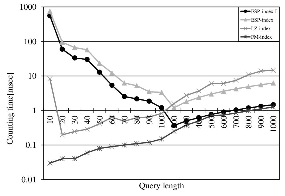
Figure 4 and 4 show the counting and locating time for query texts consisting of lengths from $10$ to $1,000$ in dna.200MB and english.200MB. In addition, the number of occurrences of query texts are presented in Figure . Since the counting and locating time of LZ-index depends quadratically on the query length, counting and locating query texts longer than 200 were slow on dna.200MB and english.200MB. SLP-index was also slow for locating query texts longer than 200, since SLP-index performs as many binary searches as query length for finding the first occurrences of variables. ESP-index-I and ESP-index were faster than LZ-index and SLP-index for counting and locating query texts, which showed that top-down searches of ESP-index-I and ESP-index for finding occurrences of variables encoding query texts were effective. ESP-index-I was from $1.4$ to $4.3$ times faster than ESP-index with respect to counting and locating time, which demonstrated our encoding of a parse tree by ESP were effective. The counting and locating time of ESP-index-I was compatitive with that of FM-index but ESP-index-I showed a higher compressibility for repetitive texts than FM-index.

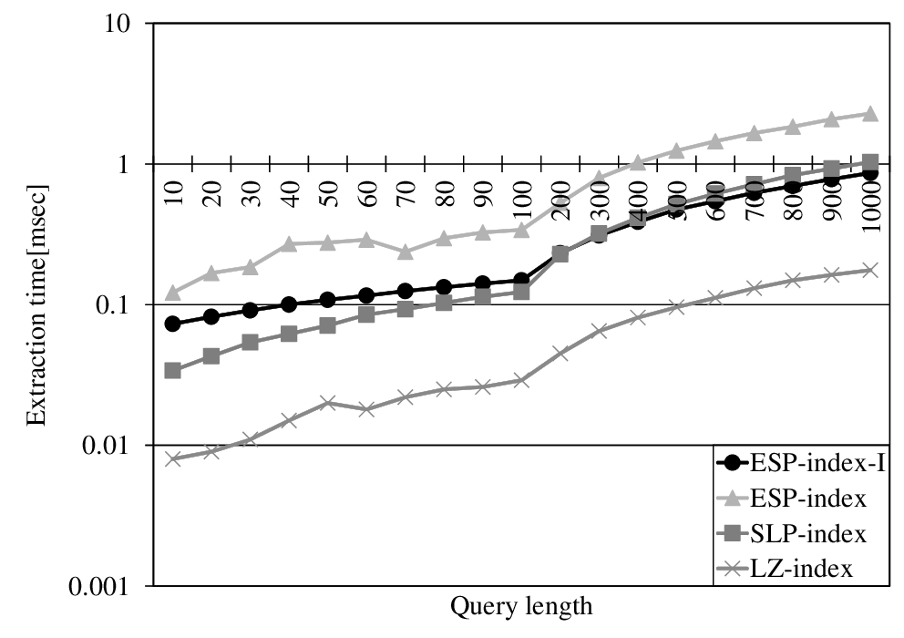
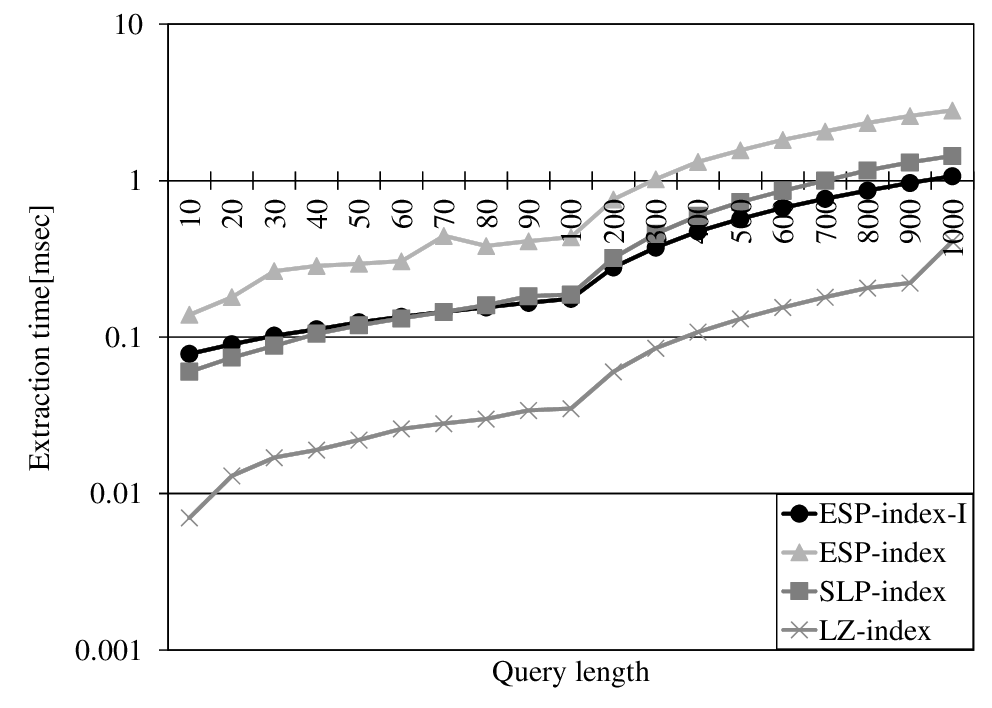
Figure 6 shows extraction time of subtexts for fixed positions and lengths. LZ-index based on LZ77 was fastest among all methods. On the otherhand, ESP-index-I was one of the fastest method among grammar-based self-indexes on dna.200MB and english.200MB.

Table 2 shows memory usage of each method in megabytes for dna.200MB and english.200MB. The methods except FM-index archived small memory, which demonstrated their high compressive abilities for texts. The memory usage of ESP-index-I was smallest among all methods, and it used 156MB and 165MB for dna.200MB and english.200MB, respectively. Since FM-index is a self-index for general texts, the memory usage of FM-index was largest among methods. Construction time is presented in Table 3.

We tried ESP-index-I on large-scale repetitive texts. The other methods except ESP-index-I did not work on these large texts, because they are applicable to only $32$ bits inputs. Table 4 shows the results for counting and locating query texts of lengths of $200$ and $1,000$, construction time and encoding size. Figure 7 shows extraction time of substring of lengths from $10$ to $1,000$. These results showed an applicability of ESP-index-I to real world repetitive texts.

References

- [1] J. Barbay and G. Navarro. On compressing permutations and adaptive sorting. Theorical Computer Science, 513:109–123, 2013.
- [2] F. Claude and G. Navarro. Self-indexed grammar-based compression. Fundamenta Informaticae, 111:313–337, 2010.
- [3] F. Claude and G. Navarro. Improved grammar-based compressed indexes. In Proceedings of the 19th Symposium on String Processing and Information Retrieval, pages 180–192, 2012.
- [4] G. Cormode and S. Muthukrishnan. The string edit distance matching problem with moves. ACM Transactions on Algorithms, 3:2:1–2:19, 2007.
- [5] O. Delpratt, N. Rahman, and R. Raman. Engineering the louds succinct tree representation. In Proceedings of the 5th International Workshop on Experimental Algorithms, pages 134–145, 2006.
- [6] T. Gagie, P. Gawrychowski, J. Kärkkäinen, and Y. Nekrich. A faster grammar-based self-index. In Proceedings of the 6th International Conference on Language and Automata Theory and Applications, pages 240–251, 2012.
- [7] T. Gagie, P. Gawrychowski, J. Kärkkäinen, Y.Nekrich, and S. J. Puglisi. LZ77-based self-indexing with faster pattern matching. In Proceedings of the 11th Latin American Theoretical Informatics Symposium, pages 731–742, 2014.
- [8] A. Golynski, J. I. Munro, and S. S. Rao. Rank/select operations on large alphabets: a tool for text indexing. In Proceedings of the 17th Annual ACM-SIAM Symposium on Discrete Algorithms, pages 368–373, 2006.
- [9] K. Goto, H. Bannai, S. Inenaga, and M. Takeda. Fast q-gram mining on SLP compressed strings. Journal of Discrete Algorithms, 18:89–99, 2013.
- [10] D. Hermelin, G.M. Landau, S. Landau, and O. Weimann. A unified algorithm for accelerating edit-distance computation via text-compression. In Proceedings of the 26th International Symposium on Theoretical Aspects of Computer Science, pages 529–540, 2009.
- [11] G. Jacobson. Space-efficient static trees and graphs. In Proceedings of the 30th Annual Symposium on Foundations of Computer Science, pages 549–554, 1989.
- [12] N.J. Larsson and A. Moffat. Off-line dictionary-based compression. In Proceedings of Data Compression Conference, pages 296–305, 1999.
- [13] S. Maruyama, M. Nakahara, N. Kishiue, and H. Sakamoto. ESP-Index: A compressed index based on edit-sensitive parsing. Journal of Discrete Algorithms, 18:100–112, 2013.
- [14] J.I. Munro, R. Raman, V. Raman, and S.S. Rao. Succinct representations of permutations. In Proceedings of the 13th International Colloquium on Automata, Languages and Programming, pages 345–356, 2003.
- [15] G. Navarro. Indexing text using the ziv-lempel trie. Journal of Discrete Algorithms, 2:87–114, 2004.
- [16] R. Raman, V. Raman, and S. S. Rao. Succinct indexable dictionaries with applications to encoding k-ary trees, prefix sums and multisets. ACM Transactions on Algorithms, 3, 2007.
- [17] H. Sakamoto, S. Maruyama, T. Kida, and S. Shimozono. A space-saving approximation algorithm for grammar-based compression. IEICE Transactions on Information and Systems, E92-D:158–165, 2009.
- [18] T. Yamamoto, H. Bannai, S. Inenaga, and M. Takeda. Faster subsequence and don’t-care pattern matching on compressed texts. In Proceedings of the 22nd Annual Symposium on Combinatorial Pattern Matching, pages 309–322, 2011.