跳到论文正文
W Papers独立论文阅读器 arXiv:1404.4788 论文正文 计算阅读时间 · 0%
引用这篇论文根据当前论文元数据生成,正式投稿前建议核对。


License: arXiv.org perpetual non-exclusive license
arXiv:1404.4788v1 [nucl-th] 18 Apr 2014

A real-time thermal field theoretical analysis of Kubo-type Shear viscosity : Numerical understanding with simple examples

Sabyasachi Ghosh
Abstract

A real-time thermal field theoretical calculation of shear viscosity has been described in the Kubo formalism for bosonic and fermionic medium. The two point function of viscous stress tensor in the lowest order provides one-loop skeleton diagram of boson or fermion field for bosonic or fermionic matter. According to the traditional diagrammatic technique of transport coefficients, the finite thermal width of boson or fermion is introduced in their internal lines during the evaluation of boson-boson or fermion-fermion loop diagram. These thermal widths of ϕ\phi boson and ψ\psi fermion are respectively obtained from the imaginary part of self-energy for ϕ​Φ\phi\Phi and ψ​Φ\psi\Phi loops, where interactions of higher mass Φ\Phi boson with ϕ\phi and ψ\psi are governed by the simple ϕ​ϕ​Φ\phi\phi\Phi and ψ¯​ψ​Φ{\overline{\psi}}\psi\Phi interaction Lagrangian densities. A two-loop diagram, having same power of coupling constant as in the one-loop diagram, is deduced and its contribution appears much lower than the one-loop values of shear viscosity. Therefore the one-loop results of Kubo-type shear viscosity may be considered as leading order results for this simple ϕ​ϕ​Φ\phi\phi\Phi and ψ¯​ψ​Φ{\overline{\psi}}\psi\Phi interactions. This approximation is valid for any values of coupling constant and at the temperatures greater than the mass of constituent particles of the medium.

1Instituto de Fisica Teorica, Universidade Estadual Paulista, Rua Dr. Bento Teobaldo Ferraz, 271, 01140-070 Sao Paulo, SP, Brazil

1 Introduction

A medium can be perturbed slightly away from its equilibrium state due to quantum fluctuations at finite temperature. The responses to these fluctuations can be determined from the dissipative quantities of the medium. The different fluxes originating from their corresponding thermodynamical forces can appear in the medium to restore the system to its equilibrium state. The transport coefficients like shear and bulk viscosities are proportional constants of the linear relations between these fluxes and forces.

With the help of Kubo formula, the transport coefficients can be microscopically estimated from their corresponding retarded thermal correlators in the low frequency limit. For example, the shear viscosity coefficient can be obtained from the retarded correlator of the viscous stress tensor. The simplest possible anatomical representation of the correlator is a one-loop kind of diagram, where a finite thermal width has to be included in the propagator of the constituent particle. This is a very well established technique [1, 2, 3, 4, 5, 6, 7], which is generally adopted to get a non-divergent value of the transport coefficient. Beyond the one-loop, there will be infinite class of planar ladder diagrams, which have the same power of coupling constant as in the one-loop diagram. The reason is that the additional coupling constants from the interaction vertices of any higher order diagram are exactly cancelled by the additional thermal widths coming from the each loop of that diagram. For this purpose, different ways of re-summed technique are proposed for ϕ4\phi^{4} theory [8, 9, 10, 11], as well as for hot QCD [12]. In this context, a Kubo-type shear viscosity calculation for medium with ϕ\phi boson or ψ\psi fermion has been derived in a generalized manner where a simple ϕ​ϕ​Φ\phi\phi\Phi or ψ​ψ​Φ\psi\psi\Phi interaction Lagrangian is considered. The Φ\Phi boson is assumed as a higher mass intermediate particle, which is supposed to be appeared in the elastic ϕ​ϕ\phi\phi or ψ​ψ\psi\psi scattering. We can take π​π​σ\pi\pi\sigma [13] or Q​Q​πQQ\pi [14] interaction as a practical example of such a case.

At first, the simplest possible diagrammatic representation of shear viscosity as a ϕ​ϕ\phi\phi or ψ​ψ\psi\psi loop is derived explicitly in the real-time thermal field theory (RTF), which is addressed in Sec. (2). For getting a non-divergent shear viscosity, a finite thermal width of ϕ\phi or ψ\psi has to be introduced owing to the traditional diagrammatic calculation of transport coefficient. In Sec. (3), the thermal width of ϕ\phi or ψ\psi is deduced from the imaginary part of its thermal self-energy for ϕ​Φ\phi\Phi or ψ​Φ\psi\Phi loop. The possibilities of different infinite number of diagrams for the ϕ​ϕ​Φ\phi\phi\Phi interaction are pointed out in Sec. (4), where a two-loop diagram is explicitly derived in RTF. During numerical estimations of one-loop and two-loop contributions in shear viscosity, two-loop is substantially suppressed due to presence of additional number of thermal distribution functions appearing in the multiplicative way. These numerical results are discussed in Sec. (5), and Sec. (6) concludes the article.

2 Formalism

From the simple derivation of Kubo formula [15, 16], we are starting our calculation with the expression of shear viscosity in momentum space [3],

η=120​limq0,q→→0Aη​(q0,q→)q0,\eta=\frac{1}{20}\lim_{q_{0},\vec{q}\rightarrow 0}\frac{A_{\eta}(q_{0},\vec{q})}{q_{0}}~, (1)

where

Aη​(q0,q→)=∫d4​x​ei​q⋅x​⟨[πi​j​(x),πi​j​(0)]⟩βA_{\eta}(q_{0},\vec{q})=\int d^{4}xe^{iq\cdot x}\langle[\pi_{ij}(x),\pi^{ij}(0)]\rangle_{\beta} (2)

is spectral function of space component of the viscous-stress tensor, πμ​ν\pi^{\mu\nu} and ⟨O^⟩β\langle\hat{O}\rangle_{\beta} for any operator O^\hat{O} denotes the equilibrium ensemble average,

⟨O^⟩β\displaystyle\langle\hat{O}\rangle_{\beta} =\displaystyle= Tr​e−β​H​O^Z\displaystyle{\rm Tr}\frac{e^{-\beta H}\hat{O}}{Z}
with​Z\displaystyle{\rm with}~~Z =\displaystyle= Tr​e−β​H.\displaystyle{\rm Tr}e^{-\beta H}~. (3)

The πμ​ν\pi^{\mu\nu} comes from the dissipative part of total energy-momentum tensor, Tμ​νT^{\mu\nu}. In the relativistic dissipative hydrodynamics [17, 18] the Tμ​νT^{\mu\nu} can be decomposed into an ideal part T0μ​νT_{0}^{\mu\nu} and a dissipative part TDμ​νT_{D}^{\mu\nu}.

i.e.Tμ​ν=T0μ​ν+TDμ​ν,{\rm\it i.e.}~~T^{\mu\nu}=T_{0}^{\mu\nu}+T_{D}^{\mu\nu}~, (4)

where

T0μ​ν\displaystyle T_{0}^{\mu\nu} =\displaystyle= ϵ​uμ​uν−P​Δμ​ν\displaystyle\epsilon u^{\mu}u^{\nu}-P\Delta^{\mu\nu}
and​TDμ​ν\displaystyle{\rm and}~~T_{D}^{\mu\nu} =\displaystyle= Kμ​uν+Kν​uμ−πμ​ν,\displaystyle K^{\mu}u^{\nu}+K^{\nu}u^{\mu}-\pi^{\mu\nu}~, (5)

with Δμ​ν=gμ​ν−uμ​uν\Delta^{\mu\nu}=g^{\mu\nu}-u^{\mu}u^{\nu} and ϵ,P,uμ\epsilon,P,u^{\mu} are respectively energy density, pressure density, four velocity of the matter. By applying appropriate projection operators, the candidates of right hand side of the Eq. (5) can be extracted from Tμ​νT^{\mu\nu} as

{ϵPKρπρ​σ}={uμ​uν−13​Δμ​νΔρ​μ​uν(Δρ​σ​Δμ​ν−13​Δρ​μ​Δσ​ν)}​Tμ​ν.\left\{\begin{array}[]{llll}\epsilon\\ P\\ K^{\rho}\\ \pi^{\rho\sigma}\end{array}\right\}=\left\{\begin{array}[]{llll}u^{\mu}u^{\nu}\\ -\frac{1}{3}\Delta^{\mu\nu}\\ \Delta^{\rho\mu}u_{\nu}\\ (\Delta^{\rho\sigma}\Delta^{\mu\nu}-\frac{1}{3}\Delta^{\rho\mu}\Delta^{\sigma\nu})\end{array}\right\}T_{\mu\nu}. (6)

For ϕ\phi boson and ψ\psi fermion the viscous-stress tensor can be deduced as (see Appendix A)

πμ​ν=(Δμρ​Δνσ−13​Δμ​ν​Δρ​σ)​{∂ρϕ​∂σϕi​ψ¯​γρ​∂σψ}.\pi_{\mu\nu}=(\Delta^{\rho}_{\mu}\Delta^{\sigma}_{\nu}-\frac{1}{3}\Delta_{\mu\nu}\Delta^{\rho\sigma})\left\{\begin{array}[]{ll}\partial_{\rho}\phi\partial_{\sigma}\phi\\ i{\overline{\psi}}\gamma_{\rho}\partial_{\sigma}\psi\end{array}\right\}~. (7)
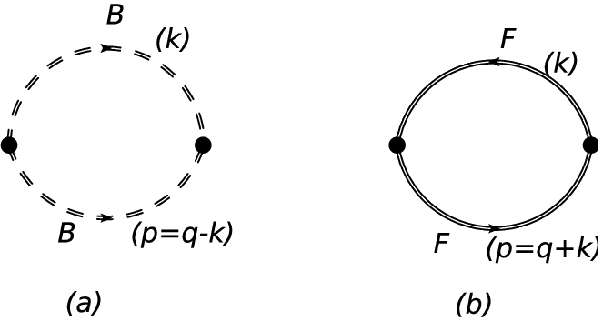
Refer to caption
Figure 1: Boson-Boson (a) and Fermion-Fermion (b) loop diagram after Wick contraction from two point function of corresponding viscus-stress tensor.

In RTF, the thermal average of any two point function always give a 2×22\times 2 matrix structure. Hence the two point correlator of viscous-stress tensor will be

Πa​b​(q)=i​∫d4​x​ei​q​x​⟨Tc​πμ​ν​(x)​πμ​ν​(0)⟩βa​b,\Pi_{ab}(q)=i\int d^{4}xe^{iqx}\langle T_{c}\pi_{\mu\nu}(x)\pi^{\mu\nu}(0)\rangle^{ab}_{\beta}~, (8)

where the superscripts a,b⁡(a,b=1,2)a,b(a,b=1,2) represent the (thermal) indices of the matrix and TcT_{c} denotes time ordering with respect to a contour in the complex time plane. Of the variety of possible contours in the complex time plane [19], two are specially interesting, namely the closed one [20] and the symmetrical one  [21, 22]. Here the latter contour is chosen .

The matrix can be diagonalized in terms of a single analytic function which determines completely the dynamics of the corresponding two point function. The diagonal element can also be related with the retarded two point function of viscous-stress tensor. These retarded function, ΠR​(q)\Pi^{R}(q) (say) or diagonal element, Π¯​(q){\overline{\Pi}}(q) (say) is simply related to any one component, say 11 component of the matrix. The relation among the imaginary part of these components (for ϕ​ϕ\phi\phi or ψ​ψ\psi\psi loops) is

Im​ΠR​(q)=ϵ⁡(q0)​Im​Π¯​(q)=tanh⁡(β​q02)​Im​Π11​(q).{\rm Im}\Pi^{R}(q)=\epsilon(q_{0}){\rm Im}{\overline{\Pi}}(q)={\rm tanh}(\frac{\beta q_{0}}{2}){\rm Im}\Pi_{11}(q)~. (9)

Now the imaginary part of retarded two point function of any field quantity is directly related with the corresponding spectral function. For our present case, the viscous-stress tensor πμ​ν\pi_{\mu\nu} is the field quantity. Hence the relation between corresponding spectral function Aη​(q)A_{\eta}(q) and retarded function ΠR​(q)\Pi^{R}(q) is given by

Aη​(q)=2​Im​ΠR​(q).A_{\eta}(q)=2{\rm Im}\Pi^{R}(q)~. (10)

Using this relation, the Eq. (1)) become

η=110​limq0,q→→0Im​ΠR​(q0,q→)q0.\eta=\frac{1}{10}\lim_{q_{0},\vec{q}\rightarrow 0}\frac{{\rm Im}\Pi^{R}(q_{0},\vec{q})}{q_{0}}~. (11)

To calculate this retarded two point function, let us start from 11 component of the Πa​b\Pi_{ab} matrix. After using Eq. (7) in Eq. (8), the Wick contraction of the boson fields (ϕ\phi) and fermion fields (ψ\psi) generate an one-loop kind of skeleton diagram, which are shown in Fig. 1(a) and (b) respectively. They can be mathematically expressed as [23]

Π11​(q)=i​ϵF​∫d4​k(2​π)4​N​(q,k)​D11​(k)​D11​(p),\Pi_{11}(q)=i\epsilon_{F}\int\frac{d^{4}k}{(2\pi)^{4}}N(q,k)D_{11}(k)D_{11}(p)~, (12)

where D11​(k)D_{11}(k) and D11​(p)D_{11}(p) are the scalar part of the propagators at finite temperature. Now p=q−kp=q-k for boson-boson (ϕ​ϕ\phi\phi) loop whereas p=q+kp=q+k for fermion-fermion (ψ​ψ\psi\psi) loop. In fermion loop there must be an extra negative sign according to Feynman rule, which is maintained by putting ϵF=+,−\epsilon_{F}=+,- for ϕ​ϕ\phi\phi and ψ​ψ\psi\psi loops respectively. The term N⁡(q,k)N(q,k) contain the numerator part of two propagators as well as the vertex kind of part which is determined from Eq. (7). The expression of N⁡(q,k)N(q,k) (multiplying with the ϵF\epsilon_{F}) for ϕ​ϕ\phi\phi and ψ​ψ\psi\psi loop are respectively given by (see Appendix B)

ϵF​N​(q,k)=−[k→2​(q→−k→)2+{k→⋅(q→−k→)}23]\epsilon_{F}N(q,k)=-[\vec{k}^{2}(\vec{q}-\vec{k})^{2}+\frac{\{\vec{k}\cdot(\vec{q}-\vec{k})\}^{2}}{3}] (13)

and

ϵF​N​(q,k)=−323​{k0​(q0+k0)}​{k→⋅(q→+k→)}+4​[{k→⋅(q→+k→)}2+k→2​(q→+k→)23].\epsilon_{F}N(q,k)=-\frac{32}{3}\{k_{0}(q_{0}+k_{0})\}\{\vec{k}\cdot(\vec{q}+\vec{k})\}+4[\{\vec{k}\cdot(\vec{q}+\vec{k})\}^{2}+\frac{\vec{k}^{2}(\vec{q}+\vec{k})^{2}}{3}]~. (14)

Just by absorbing the ϵF\epsilon_{F} in N⁡(q,k)N(q,k) we will not write it for our further calculations.

In RTF, the 11 component of the scalar part of the thermal propagator can be expressed as

D11​(k)\displaystyle D^{11}(k) =\displaystyle= −1k02−ωk2+i​ϵ+2​π​i​ϵk​Fk​(k0)​δ​(k02−ωk2),with​Fk​(k0)=nk+​θ​(k0)+nk−​θ​(−k0)\displaystyle\frac{-1}{k_{0}^{2}-\omega_{k}^{2}+i\epsilon}+2\pi i\epsilon_{k}F_{k}(k_{0})\delta(k_{0}^{2}-\omega_{k}^{2}),~{\rm with}~F_{k}(k_{0})=n^{+}_{k}\theta(k_{0})+n^{-}_{k}\theta(-k_{0}) (15)
=\displaystyle= −12​ωk​(1−nk+k0−ωk+i​ϵ+nk+k0−ωk−i​ϵ−1−nk−k0+ωk−i​ϵ−nk−k0+ωk+i​ϵ).\displaystyle-\frac{1}{2\omega_{k}}(\frac{1-n^{+}_{k}}{k_{0}-\omega_{k}+i\epsilon}+\frac{n^{+}_{k}}{k_{0}-\omega_{k}-i\epsilon}-\frac{1-n^{-}_{k}}{k_{0}+\omega_{k}-i\epsilon}-\frac{n^{-}_{k}}{k_{0}+\omega_{k}+i\epsilon})~.

Here nk±​(ωk)=1eβ⁡(ωk∓μ)−ϵkn^{\pm}_{k}(\omega_{k})=\frac{1}{e^{\beta(\omega_{k}\mp\mu)}-\epsilon_{k}} (ϵk=+1,−1\epsilon_{k}=+1,-1 for ϕ\phi and ψ\psi respectively) is the thermal distribution of ϕ\phi with energy ωk=(k→2+mϕ2)1/2\omega_{k}=(\vec{k}^{2}+m_{\phi}^{2})^{1/2} or ψ\psi with energy ωk=(k→2+mψ2)1/2\omega_{k}=(\vec{k}^{2}+m_{\psi}^{2})^{1/2}, where the ±\pm sign in the superscript of nkn_{k} refer to particle and anti-particle respectively.

After doing the k0k_{0} integration of Eq. (12) and then using the relations (9), we get the imaginary part of retarded self-energy [24]

Im​ΠR​(q)\displaystyle{\rm Im}{\Pi}^{R}(q) =\displaystyle= ∫d3​k(2​π)3(−π)​N4​ωk​ωp[C1δ(q0−ωk−ωp)+C2δ(q0−ωk+ωp)\displaystyle\int\frac{d^{3}k}{(2\pi)^{3}}\frac{(-\pi)N}{4\omega_{k}\omega_{p}}[C_{1}\delta(q_{0}-\omega_{k}-\omega_{p})+C_{2}\delta(q_{0}-\omega_{k}+\omega_{p}) (16)
+C3δ(q0+ωk−ωp)+C4δ(q0+ωk+ωp)],\displaystyle+C_{3}\delta(q_{0}+\omega_{k}-\omega_{p})+C_{4}\delta(q_{0}+\omega_{k}+\omega_{p})]~,

where ωp=(q→∓k→)2+m2\omega_{p}=\sqrt{(\vec{q}\mp\vec{k})^{2}+m^{2}} (∓\mp for ϕ​ϕ\phi\phi and ψ​ψ\psi\psi loop respectively) and N=N⁡(k0=±ωk,k→,q)N=N(k_{0}=\pm\omega_{k},\vec{k},q) . Here Ci(i=1,..,4)C_{i}(i=1,..,4) are four different statistical probability attached with four different delta functions. For ϕ​ϕ\phi\phi loop, Ci(i=1,..,4)={1+nk+(ωk)+np+(q0−ωk)}C_{i}(i=1,..,4)=\{1+n^{+}_{k}(\omega_{k})+n^{+}_{p}(q_{0}-\omega_{k})\}, {−nk+​(ωk)+np−​(−q0+ωk)}\{-n^{+}_{k}(\omega_{k})+n^{-}_{p}(-q_{0}+\omega_{k})\}, {nk−​(ωk)−np+​(q0+ωk)}\{n^{-}_{k}(\omega_{k})-n^{+}_{p}(q_{0}+\omega_{k})\}, {−1−nk−​(ωk)−np−​(−q0−ωk)}\{-1-n^{-}_{k}(\omega_{k})-n^{-}_{p}(-q_{0}-\omega_{k})\} whereas Ci(i=1,..,4)={−1+nk−(ωk)+np+(q0+ωk)}C_{i}(i=1,..,4)=\{-1+n^{-}_{k}(\omega_{k})+n^{+}_{p}(q_{0}+\omega_{k})\}, {−nk−​(ωk)+np−​(−q0+ωk)}\{-n^{-}_{k}(\omega_{k})+n^{-}_{p}(-q_{0}+\omega_{k})\}, {nk+​(ωk)−np+​(q0+ωk)}\{n^{+}_{k}(\omega_{k})-n^{+}_{p}(q_{0}+\omega_{k})\}, {1−nk+​(ωk)−np−​(−q0−ωk)}\{1-n^{+}_{k}(\omega_{k})-n^{-}_{p}(-q_{0}-\omega_{k})\} for ψ​ψ\psi\psi loop. Four different branch cuts in the real axis of complex q0q_{0} plane can be identified from four different terms of Im​ΠR​(q){\rm Im}{\Pi}^{R}(q) with different delta functions. In addition to the unitary cut, present already in vacuum, the thermal field theory calculation generates a new cut, the so called the Landau cut. The region of these different branch cuts are (−∞-\infty to −q→2+4​mϕ,ψ2-\sqrt{\vec{q}^{2}+4m_{\phi,\psi}^{2}}) for unitary cut in negative q0q_{0}-axis, (−q→-\vec{q} to q→\vec{q}) for Landau cut and (q→2+4​mϕ,ψ2\sqrt{\vec{q}^{2}+4m_{\phi,\psi}^{2}} to ∞\infty) for unitary cut in positive q0q_{0}-axis. Now to calculate η\eta from the ΠR​(q){\Pi}^{R}(q), we have to concentrate on the limit of q0,q→→0q_{0},\vec{q}\rightarrow 0. Therefore the Landau cuts will be only the focus of our calculation. Hence using the Landau part of Eq. (16) in Eq. (11), we have

η\displaystyle\eta =\displaystyle= 110​limq0,q→→01q0​∫d3​k(2​π)3​(−π)​N4​ωk​ωp​{C2​δ​(q0−ωk+ωp)+C3​δ​(q0+ωk−ωp)}\displaystyle\frac{1}{10}\lim_{q_{0},\vec{q}\rightarrow 0}\frac{1}{q_{0}}\int\frac{d^{3}k}{(2\pi)^{3}}\frac{(-\pi)N}{4\omega_{k}\omega_{p}}\{C_{2}\delta(q_{0}-\omega_{k}+\omega_{p})+C_{3}\delta(q_{0}+\omega_{k}-\omega_{p})\} (17)
=\displaystyle= 110limq0,q→→0Im[∫d3​k(2​π)3N4​ωk​ωplimΓ→0\displaystyle\frac{1}{10}\lim_{q_{0},\vec{q}\rightarrow 0}{\rm Im}\left[\int\frac{d^{3}k}{(2\pi)^{3}}\frac{N}{4\omega_{k}\omega_{p}}\lim_{\Gamma\rightarrow 0}\right.
{C2/q0(q0−ωk+ωp)+i​Γ+C3/q0(q0+ωk−ωp)+i​Γ}].\displaystyle\left.\left\{\frac{C_{2}/q_{0}}{(q_{0}-\omega_{k}+\omega_{p})+i\Gamma}+\frac{C_{3}/q_{0}}{(q_{0}+\omega_{k}-\omega_{p})+i\Gamma}\right\}\right]~.

To get a non-divergent contribution of η\eta, the further calculation will be continued for finite value of Γ\Gamma. This is the place where the interaction scenario is introduced, which is very essential for a dissipative system. This is done by transforming the delta functions for free theory to the spectral functions with finite thermal width for interacting theory. The Γ\Gamma is identified as the thermal width (or collision rate) of the constituent particles and it reciprocally measures the dissipative coefficients like the shear viscosity. In this respect this formalism may be equivalent to quasi particle approximation and this trained is widely used for calculating the dissipative coefficients in Kubo approach [3, 6]. Using the limiting values,

limq→→0ωp=ωk\lim_{\vec{q}\rightarrow 0}\omega_{p}=\omega_{k} (18)

in Eq. (17), we have

η=110​∫d3​k(2​π)3​(−N0)4​ωk2​Γ​[I2+I3],\eta=\frac{1}{10}\int\frac{d^{3}k}{(2\pi)^{3}}\frac{(-N^{0})}{4\omega_{k}^{2}\Gamma}[I_{2}+I_{3}]~, (19)

where

N0=limq0,q→→0N⁡(k0=±ωk,k→,q)N^{0}=\lim_{q_{0},\vec{q}\rightarrow 0}N(k_{0}=\pm\omega_{k},\vec{k},q) (20)

and

I2,3=limq0→0C2,3​(q0)q0,I_{2,3}=\lim_{q_{0}\rightarrow 0}\frac{C_{2,3}(q_{0})}{q_{0}}~, (21)

with

C2,3​(q0)=∓nk±​(ωk)±np∓​(∓q0+ωk).C_{2,3}(q_{0})=\mp n^{\pm}_{k}(\omega_{k})\pm n^{\mp}_{p}(\mp q_{0}+\omega_{k})~. (22)

Here in Eq. (21), we see that the limiting value of I2,3I_{2,3} is appeared to be a 0/00/0 form and so we can apply the L’Hospital’s rule i.e.

I2,3\displaystyle I_{2,3} =\displaystyle= limq0→0dd​q0​{C2,3​(q0)}dd​q0​{q0}\displaystyle\lim_{q_{0}\rightarrow 0}\frac{\frac{d}{dq_{0}}\{C_{2,3}(q_{0})\}}{\frac{d}{dq_{0}}\{q_{0}\}} (23)
=\displaystyle= β​nk∓​(1+ϵk​nk∓),\displaystyle\beta n_{k}^{\mp}(1+\epsilon_{k}n^{\mp}_{k})~,

since

dd​q0​{±np∓​(ωq=∓q0+ωk)}\displaystyle\frac{d}{dq_{0}}\{\pm n^{\mp}_{p}(\omega_{q}=\mp q_{0}+\omega_{k})\} =\displaystyle= ±−β​d​ωqd​q0​eβ⁡(ωq±μ){eβ⁡(ωq±μ)−ϵk}2\displaystyle\pm\frac{-\beta\frac{d\omega_{q}}{dq_{0}}e^{\beta(\omega_{q}\pm\mu)}}{\{e^{\beta(\omega_{q}\pm\mu)}-\epsilon_{k}\}^{2}}
limq0→0dd​q0​{±np∓​(ωq=∓q0+ωk)}\displaystyle\lim_{q_{0}\rightarrow 0}\frac{d}{dq_{0}}\{\pm n^{\mp}_{p}(\omega_{q}=\mp q_{0}+\omega_{k})\} =\displaystyle= ±−β⁡(∓)​eβ⁡(ωk±μ){eβ⁡(ωk±μ)−ϵk}2\displaystyle\pm\frac{-\beta(\mp)e^{\beta(\omega_{k}\pm\mu)}}{\{e^{\beta(\omega_{k}\pm\mu)}-\epsilon_{k}\}^{2}} (24)
=\displaystyle= β⁡[nk±​(1+ϵk​nk±)].\displaystyle\beta[n^{\pm}_{k}(1+\epsilon_{k}n^{\pm}_{k})]~.

Depending on the sign of ϵk\epsilon_{k}, the statistical probability become Bose enhanced (ϵk=+1\epsilon_{k}=+1 for ϕ\phi) or Pauli blocked (ϵk=−1\epsilon_{k}=-1 for ψ\psi) probability. Hence using Eq. (23) in Eq. (19), we can get a generalized expression of shear viscosity coefficient for ϕ\phi boson or ψ\psi fermion,

η\displaystyle\eta =\displaystyle= β10​∫d3​k(2​π)3​(−N0)4​ωk2​Γ​[nk−​(1+ϵk​nk−)+nk+​(1+ϵk​nk+)]\displaystyle\frac{\beta}{10}\int\frac{d^{3}k}{(2\pi)^{3}}\frac{(-N^{0})}{4\omega_{k}^{2}\Gamma}[n^{-}_{k}(1+\epsilon_{k}n^{-}_{k})+n^{+}_{k}(1+\epsilon_{k}n^{+}_{k})] (25)
=\displaystyle= β80​π2​∫k→2​d​k→ωk2​(−N0)Γ​[nk−​(1+ϵk​nk−)+nk+​(1+ϵk​nk+)].\displaystyle\frac{\beta}{80\pi^{2}}\int\frac{\vec{k}^{2}d\vec{k}}{\omega_{k}^{2}}\frac{(-N^{0})}{\Gamma}[n^{-}_{k}(1+\epsilon_{k}n^{-}_{k})+n^{+}_{k}(1+\epsilon_{k}n^{+}_{k})]~.

From the final expression we can understand the importance of finite value of Γ\Gamma to get a non-divergent value of η\eta. A finite small value of Γ\Gamma can be introduced through Dyson’s series expansion of a propagator and we can repeat our calculation from Eq. (15) by using i​Γi\Gamma in place of i​ηi\eta. The corresponding Γ\Gamma for ϕ\phi and ψ\psi can be quantitatively defined as

Γϕ=−ImΠ(ϕ)R(k0=ωk,k→)/mϕ(forϕ),\Gamma_{\phi}=-{\rm Im}{\Pi}^{R}_{(\phi)}(k_{0}=\omega_{k},\vec{k})/m_{\phi}~~~~~({\rm for~}\phi)~, (26)
Γψ=−Im​Σ(ψ)R​(k0=ωk,k→)(for​ψ),\Gamma_{\psi}=-{\rm Im}\Sigma^{R}_{(\psi)}(k_{0}=\omega_{k},\vec{k})~~~~~~~~~~({\rm for~}\psi)~, (27)

where Im​Π(ϕ)R​(k){\rm Im}{\Pi}^{R}_{(\phi)}(k) and Im​Σ(ψ)R​(k){\rm Im}\Sigma^{R}_{(\psi)}(k) are the imaginary part of retarded self-energy for ϕ\phi and ψ\psi respectively, which will be even functions of k0k_{0}.

Let us now concentrate on the Eq. (20) to deduce N0N^{0}. In this limiting case (q0,q→→0q_{0},\vec{q}\rightarrow 0), the Eq. (13) and (14) can be simplified as

N0=−4​k→43​for​ϕ​ϕ​loopN^{0}=-\frac{4\vec{k}^{4}}{3}~~~{\rm for~}\phi\phi~{\rm loop} (28)

and

N0=−16​k→43​for​ψ​ψ​loop.N^{0}=-\frac{16\vec{k}^{4}}{3}~~~{\rm for~}\psi\psi~{\rm loop}~. (29)

Hence the shear viscosity of the medium with bosons (ϕ\phi) and fermions (ψ\psi) are respectively given below

ηϕ\displaystyle\eta_{\phi} =\displaystyle= β30​π2​∫0∞d​k→​k→6ωk2​Γϕ​{nk+​(1+nk+)+nk−​(1+nk−)}2​for​ϕ​ϕ​loop\displaystyle\frac{\beta}{30\pi^{2}}\int^{\infty}_{0}\frac{d\vec{k}\vec{k}^{6}}{\omega_{k}^{2}\Gamma_{\phi}}\frac{\{n^{+}_{k}(1+n^{+}_{k})+n^{-}_{k}(1+n^{-}_{k})\}}{2}~~~{\rm for~}\phi\phi~{\rm loop} (30)
=\displaystyle= β30​π2​∫0∞d​k→​k→6ωk2​Γϕ​nk​(1+nk)(at​μ=0)\displaystyle\frac{\beta}{30\pi^{2}}\int^{\infty}_{0}\frac{d\vec{k}\vec{k}^{6}}{\omega_{k}^{2}\Gamma_{\phi}}n_{k}(1+n_{k})~~~~~~~({\rm at}~\mu=0)

and

ηψ=β15​π2​∫0∞d​k→​k→6ωk2​Γψ​{nk+​(1−nk+)+nk−​(1−nk−)}​for​ψ​ψ​loop.\eta_{\psi}=\frac{\beta}{15\pi^{2}}\int^{\infty}_{0}\frac{d\vec{k}\vec{k}^{6}}{\omega_{k}^{2}\Gamma_{\psi}}\{n^{+}_{k}(1-n^{+}_{k})+n^{-}_{k}(1-n^{-}_{k})\}~~~{\rm for~}\psi\psi~{\rm loop}~. (31)

Some special cases : Now taking isospin degeneracy factor Iπ=3I_{\pi}=3 for pionic medium we can generate the expression of  [3, 6, 22, 23],

ηπ=β10​π2​∫0∞d​k→​k→6ωk2​Γπ​nk​(1+nk),\eta_{\pi}=\frac{\beta}{10\pi^{2}}\int^{\infty}_{0}\frac{d\vec{k}\vec{k}^{6}}{\omega_{k}^{2}\Gamma_{\pi}}n_{k}(1+n_{k})~, (32)

where nk=nk±n_{k}=n^{\pm}_{k} for μπ=0\mu_{\pi}=0 has to be considered. This one-loop expression of shear viscosity from Kubo approach [3, 6, 23] is exactly coincide with the expressions from the relaxation-time approximation of the kinetic theory approach [25, 26, 27, 23].

When the constituent particles are nucleon, then we have to take isospin degeneracy IN=2I_{N}=2 in Eq. (31) i.e.

ηN=2​β15​π2​∫0∞d​k→​k→6ωk2​ΓN​{nk+​(1−nk+)+nk−​(1−nk−)}.\eta_{N}=\frac{2\beta}{15\pi^{2}}\int^{\infty}_{0}\frac{d\vec{k}\vec{k}^{6}}{\omega_{k}^{2}\Gamma_{N}}\{n^{+}_{k}(1-n^{+}_{k})+n^{-}_{k}(1-n^{-}_{k})\}~. (33)

Similarly for 2-flavor (Nf=2N_{f}=2) quark matter the degeneracy factor become Nf​Nc=6N_{f}N_{c}=6 (as color degeneracy Nc=3N_{c}=3) and so

ηQ=2​β5​π2​∫0∞d​k→​k→6ωk2​ΓQ​{nk+​(1−nk+)+nk−​(1−nk−)}.\eta_{Q}=\frac{2\beta}{5\pi^{2}}\int^{\infty}_{0}\frac{d\vec{k}\vec{k}^{6}}{\omega_{k}^{2}\Gamma_{Q}}\{n^{+}_{k}(1-n^{+}_{k})+n^{-}_{k}(1-n^{-}_{k})\}~. (34)

This expression is also exactly coincide with the expressions from the relaxation-time approximation [28].

3 Calculation of Γ\Gamma

Let us take a simple ϕ3\phi^{3}-type interaction Lagrangian density,

ℒ=−g​ϕ​ϕ​Φ,{\cal L}=-g\phi\phi\Phi~, (35)

by which we can get an estimation of Γϕ\Gamma_{\phi} for boson constituent particle, ϕ\phi.

Refer to caption
Figure 2: Self-energy of ϕ\phi boson for ϕ​Φ\phi\Phi loop (a) and self-energy of ψ\psi fermion for ψ​Φ\psi\Phi loop (b).

The Φ\Phi is another higher mass boson like ϕ\phi. The self-energy of ϕ\phi for ϕ​Φ\phi\Phi loop (as shown in Fig. 2(a)) can be derived in RTF with the help of the above Lagrangian. Owing to the cutkosky rule at finite TT, the Γϕ\Gamma_{\phi} can be extracted from the imaginary part of this one-loop self-energy of ϕ\phi at its pole, which is already expressed in Eq. (26).

For estimating Γϕ\Gamma_{\phi}, we have to repeat a similar calculations as previously done in one-loop calculation for η\eta. Therefore Let us start from 11 component of self-energy of ϕ\phi for ϕ​Φ\phi\Phi loop,

Π(ϕ)11(k)=−i∫d4​l(2​π)4L(k,l)D11(l,mϕ)D11(u=k−l,mΦ),\Pi^{11}_{(\phi)}(k)=-i\int\frac{d^{4}l}{(2\pi)^{4}}L(k,l)D_{11}(l,m_{\phi})D_{11}(u=k-l,m_{\Phi})~, (36)

where D11​(l,mϕ)D_{11}(l,m_{\phi}) and D11​(u=k−l,mΦ)D_{11}(u=k-l,m_{\Phi}) are the scalar part of ϕ\phi and Φ\Phi propagators at finite temperature with similar form like Eq. (15).

Similar to Eq. (16), we will get the imaginary part of retarded self-energy for the ϕ​Φ\phi\Phi loop,

Im​Π(ϕ)R​(k)\displaystyle{\rm Im}{\Pi}^{R}_{(\phi)}(k) =\displaystyle= π∫d3​l(2​π)314​ωl​ωu[L(l0=ωl,l→,k)[{1+nl(ωl)+nu(k0−ωl)}δ(k0−ωl−ωu)\displaystyle\pi\int\frac{d^{3}l}{(2\pi)^{3}}\frac{1}{4\omega_{l}\omega_{u}}[L(l_{0}=\omega_{l},{\vec{l}},k)[\{1+n_{l}(\omega_{l})+n_{u}(k_{0}-\omega_{l})\}\delta(k_{0}-\omega_{l}-\omega_{u}) (37)
+{−nl(ωl)+nu(−k0+ωl)}δ(k0−ωl+ωu)]\displaystyle~~~~~~~~~~~+\{-n_{l}(\omega_{l})+n_{u}(-k_{0}+\omega_{l})\}\delta(k_{0}-\omega_{l}+\omega_{u})]
+L(l0=−ωl,l→,k)[{nl(ωl)−nu(k0+ωl)}δ(k0+ωl−ωu)\displaystyle+L(l_{0}=-\omega_{l},{\vec{l}},k)[\{n_{l}(\omega_{l})-n_{u}(k_{0}+\omega_{l})\}\delta(k_{0}+\omega_{l}-\omega_{u})
+{−1−nl(ωl)−nu(−k0−ωl)}δ(k0+ωl+ωu)],\displaystyle~~~~~~~~~~~+\{-1-n_{l}(\omega_{l})-n_{u}(-k_{0}-\omega_{l})\}\delta(k_{0}+\omega_{l}+\omega_{u})]~,

where ωu=(k→−l→)2+mΦ2\omega_{u}=\sqrt{({\vec{k}}-{\vec{l}})^{2}+m_{\Phi}^{2}} and n′n^{\prime}s are Bose-Einstein distribution functions. The region of the different branch cuts in k0k_{0}-axis are (−∞-\infty to −k→2+(mΦ+mϕ)2-\sqrt{\vec{k}^{2}+(m_{\Phi}+m_{\phi})^{2}}) for unitary cut in negative k0k_{0}-axis, (−k→2+(mΦ−mϕ)2-\sqrt{\vec{k}^{2}+(m_{\Phi}-m_{\phi})^{2}} to k→2+(mΦ−mϕ)2\sqrt{\vec{k}^{2}+(m_{\Phi}-m_{\phi})^{2}}) for Landau cut and (k→2+(mΦ+mϕ)2\sqrt{\vec{k}^{2}+(m_{\Phi}+m_{\phi})^{2}} to ∞\infty) for unitary cut in positive k0k_{0}-axis. These are the different off-shell regions of ϕ\phi boson, where imaginary part of its self-energy acquires a non-zero values because of the different δ\delta functions in Eq. (37). One can notice that the ϕ\phi pole will remain within the Landau cuts only when mΦ>2​mϕm_{\Phi}>2m_{\phi}. Hence we take an ad hoc assumption mΦ=3​mϕm_{\Phi}=3m_{\phi} to satisfy the threshold condition.

According to Eq. (26), the Γϕ\Gamma_{\phi} will be coming from Landau cut contribution associated with the third term of Eq. (37), which can be simplified as

Γϕ=116​π​k→​mϕ​∫ω~+ω~−d​ω~​L​(l0=−ω~,l→=ω~2−mϕ2,k0=ωk,k→)​{nl​(ω~)−nu​(ωk+ω~)},\Gamma_{\phi}=\frac{1}{16\pi\vec{k}m_{\phi}}\int^{\widetilde{\omega}^{-}}_{\widetilde{\omega}^{+}}d\widetilde{\omega}L(l_{0}=-\widetilde{\omega},{\vec{l}}=\sqrt{\widetilde{\omega}^{2}-m_{\phi}^{2}},k_{0}=\omega_{k},\vec{k})\{n_{l}(\widetilde{\omega})-n_{u}(\omega_{k}+\widetilde{\omega})\}~, (38)

where ω~±=R22​mϕ2​(−ωk±k→​W)\widetilde{\omega}^{\pm}=\frac{R^{2}}{2m_{\phi}^{2}}(-\omega_{k}\pm\vec{k}W) with ωk=k→2+mϕ2\omega_{k}=\sqrt{\vec{k}^{2}+m_{\phi}^{2}}, W=1−4​mϕ4R4W=\sqrt{1-\frac{4m_{\phi}^{4}}{R^{4}}} and R2=2​mϕ2−mΦ2R^{2}=2m_{\phi}^{2}-m_{\Phi}^{2}.

Now to estimate Γψ\Gamma_{\psi} of ψ\psi fermion, let us take a similar kind of interaction Lagrangian density,

ℒ=−G​ψ¯​ψ​Φ,{\cal L}=-G{\overline{\psi}}\psi\Phi~, (39)

where the mass of the Φ\Phi boson is again assumed to be three times larger than the mass of the ψ\psi fermion i.e. mΦ=3​mψm_{\Phi}=3m_{\psi}. The self-energy of ψ\psi, Σ(ψ)​(k)\Sigma_{(\psi)}(k) for ψ​Φ\psi\Phi loop is shown in Fig. 2(b). According to Eq. (27), we get

Γψ=116​π​k→​∫ω~+ω~−d​ω~​L​(l0=−ω~,l→=ω~2−mψ2,k0=ωk,k→)​{nl−​(ω~)+nu​(ωk+ω~)},\Gamma_{\psi}=\frac{1}{16\pi\vec{k}}\int^{\widetilde{\omega}^{-}}_{\widetilde{\omega}^{+}}d\widetilde{\omega}L(l_{0}=-\widetilde{\omega},{\vec{l}}=\sqrt{\widetilde{\omega}^{2}-m_{\psi}^{2}},k_{0}=\omega_{k},\vec{k})\{n^{-}_{l}(\widetilde{\omega})+n_{u}(\omega_{k}+\widetilde{\omega})\}~, (40)

which is very similar to Eq. (38). The modified parameters are ω~±=R22​mψ2​(−ωk±k→​W)\widetilde{\omega}^{\pm}=\frac{R^{2}}{2m_{\psi}^{2}}(-\omega_{k}\pm\vec{k}W) with ωk=k→2+mψ2\omega_{k}=\sqrt{\vec{k}^{2}+m_{\psi}^{2}}, W=1−4​mψ4R4W=\sqrt{1-\frac{4m_{\psi}^{4}}{R^{4}}} and R2=2​mψ2−mΦ2R^{2}=2m_{\psi}^{2}-m_{\Phi}^{2}. Here nl−n^{-}_{l} is Fermi-Dirac distribution function of anti-fermion and nun_{u} is Bose-Einstein distribution function of Φ\Phi boson.

The vertex part L⁡(k,l)L(k,l) for these loops are respectively given below

L⁡(k,l)=−g2​(for​ϕ​Φ​loop),L(k,l)=-g^{2}~~~({\rm for}~\phi\Phi~{\rm loop})~, (41)
L⁡(k,l)=−G2​mψ​(for​ψ​Φ​loop).L(k,l)=-G^{2}m_{\psi}~~~({\rm for}~\psi\Phi~{\rm loop})~. (42)

4 Higher order loop diagrams

As Γϕ∝g2\Gamma_{\phi}\propto g^{2} (or Γψ∝G2\Gamma_{\psi}\propto G^{2}), hence our one-loop contribution of two point viscous stress tensor will be 𝒪⁡(1/g2){\cal O}(1/g^{2}) (since η∝𝒪⁡(1/Γϕ)\eta\propto{\cal O}(1/\Gamma_{\phi})). Now there are some higher order loop diagrams which are also 𝒪⁡(1/g2){\cal O}(1/g^{2}). First possible digram is shown in the Fig. 3(a) which contain two loops and two ϕ​ϕ​Φ\phi\phi\Phi vertex vϕ​ϕ​Φ∝gv_{\phi\phi\Phi}\propto g. Therefore its order will be 𝒪⁡(1Γ2​vϕ​ϕ​Φ2)=𝒪⁡(1/g2){\cal O}(\frac{1}{\Gamma^{2}}v_{\phi\phi\Phi}^{2})={\cal O}(1/g^{2}) (as 1/Γ1/\Gamma will be coming from each loop). Similarly we can get same order from the diagram, shown in the Fig. 3(b), which contain (n+1)(n+1) number of loops and 2​n2n number of vϕ​ϕ​Φv_{\phi\phi\Phi}. Even for n=∞n=\infty we get same order of contribution.

Refer to caption
Figure 3: two loops (a) and (n+1) loops (b) ladder type diagrams for ϕ​ϕ​Φ\phi\phi\Phi interaction.
Refer to caption
Figure 4: The four possible combinations for two loop diagrams in RTF. The Π12A​B\Pi^{AB}_{12} is the combinations of diagrams (a) and (b) whereas diagrams (c) and (d) are combined in Π12C​D\Pi^{CD}_{12}.
Refer to caption
Figure 5: two loops (a) and (n+1) loops (b) rung type diagrams for ϕ​ϕ​Φ\phi\phi\Phi interaction.

Let us first derive the two-loop digram (Fig. 3(a)) to get a numerical estimation, which can be compared with the contributions of one-loop diagram. Instead of 11 component we will deduce the 12 component for some certain advantage to simplify our calculation. As any one of the four component in RTF can be expressed in terms of the diagonal element Π¯{\overline{\Pi}} due to their relation

(Π11Π12Π21Π22)=(1+n−n−n1+n)​(Π¯00−Π¯∗)​(1+n−n−n1+n).\left(\begin{array}[]{cc}\Pi_{11}&\Pi_{12}\\ \Pi_{21}&\Pi_{22}\end{array}\right)=\left(\begin{array}[]{cc}\sqrt{1+n}&-\sqrt{n}\\ -\sqrt{n}&\sqrt{1+n}\end{array}\right)\left(\begin{array}[]{cc}{\overline{\Pi}}&0\\ 0&-{\overline{\Pi}}^{*}\end{array}\right)\left(\begin{array}[]{cc}\sqrt{1+n}&-\sqrt{n}\\ -\sqrt{n}&\sqrt{1+n}\end{array}\right)~. (43)

Therefore we can express the shear viscosity in terms of 12 component of two-loop skeleton digram as

η(2)=110​limq0,q→→0ϵ⁡(q0)​Im​Π¯(2)​(q0,q→)q0=110​limq0,q→→0sinh⁡(β​q0/2)q0​Im​Π12(2)​(q0,q→).\eta^{(2)}=\frac{1}{10}\lim_{q_{0},\vec{q}\rightarrow 0}\frac{\epsilon(q_{0}){\rm Im}{\overline{\Pi}}^{(2)}(q_{0},\vec{q})}{q_{0}}=\frac{1}{10}\lim_{q_{0},\vec{q}\rightarrow 0}\frac{{\rm sinh}(\beta q_{0}/2)}{q_{0}}{\rm Im}\Pi^{(2)}_{12}(q_{0},\vec{q})~. (44)

Applying L’Hospital’s rule, we have

limq0→0sinh⁡(β​q0/2)q0\displaystyle\lim_{q_{0}\rightarrow 0}\frac{{\rm sinh}(\beta q_{0}/2)}{q_{0}} =\displaystyle= limq0→0dd​q0​{sinh⁡(β​q0/2)}dd​q0​{q0}\displaystyle\lim_{q_{0}\rightarrow 0}\frac{\frac{d}{dq_{0}}\{{\rm sinh}(\beta q_{0}/2)\}}{\frac{d}{dq_{0}}\{q_{0}\}} (45)
=\displaystyle= β2\displaystyle\frac{\beta}{2}

and so

η(2)=β20​limq0,q→→0Im​Π12(2)​(q0,q→).\eta^{(2)}=\frac{\beta}{20}\lim_{q_{0},\vec{q}\rightarrow 0}{\rm Im}\Pi^{(2)}_{12}(q_{0},\vec{q})~. (46)

Denoting the intermediate vertices vϕ​ϕ​Φv_{\phi\phi\Phi} in four possible way as shown in Fig. (4), we get the 12 component as a summation of four possible diagrams. By attaching different momentum labels on the internal lines, the four terms can be merged into two as given below [29]

i​Π12(2)​(q)=i​Π12A​B​(q)+i​Π12C​D​(q),i\Pi^{(2)}_{12}(q)=i\Pi^{AB}_{12}(q)+i\Pi^{CD}_{12}(q)~, (47)

where

iΠ12A​B(q)=−i∫d4​k​d4​l(2​π)8N(2)(q,k,l)D12ϕ(l)D21ϕ(r=q−l)DA​B,i\Pi^{AB}_{12}(q)=-i\int\frac{d^{4}kd^{4}l}{(2\pi)^{8}}N^{(2)}(q,k,l)D^{\phi}_{12}(l)D^{\phi}_{21}(r=q-l)D^{AB}~, (48)
i​Π12C​D​(q)=i​∫d4​k​d4​l(2​π)8​N(2)​(q,k,l)​D12ϕ​(l)​D21ϕ​(p=q−k)​D12Φ​(u=k−l)​DC​D,i\Pi^{CD}_{12}(q)=i\int\frac{d^{4}kd^{4}l}{(2\pi)^{8}}N^{(2)}(q,k,l)D^{\phi}_{12}(l)D^{\phi}_{21}(p=q-k)D^{\Phi}_{12}(u=k-l)D^{CD}~, (49)

with

DA​B\displaystyle D^{AB} =\displaystyle= {D11ϕ​(k)​D11ϕ​(p=q−k)​D11Φ​(u=k−l)+D22ϕ​(k)​D22ϕ​(p=q−k)​D22Φ​(u=k−l)}\displaystyle\{D^{\phi}_{11}(k)D^{\phi}_{11}(p=q-k)D^{\Phi}_{11}(u=k-l)+D^{\phi}_{22}(k)D^{\phi}_{22}(p=q-k)D^{\Phi}_{22}(u=k-l)\} (50)
=\displaystyle= 2​i​Im​{D11ϕ​(k)​D11ϕ​(p=q−k)​D11Φ​(u=k−l)},\displaystyle 2i{\rm Im}\{D^{\phi}_{11}(k)D^{\phi}_{11}(p=q-k)D^{\Phi}_{11}(u=k-l)\}~,
DC​D\displaystyle D^{CD} =\displaystyle= {D11ϕ​(k)​D22ϕ​(r=q−l)+D22ϕ​(k)​D11ϕ​(r=q−l)}\displaystyle\{D^{\phi}_{11}(k)D^{\phi}_{22}(r=q-l)+D^{\phi}_{22}(k)D^{\phi}_{11}(r=q-l)\} (51)
=\displaystyle= 2​R​e​{D11ϕ​(k)​D22ϕ​(r=q−l)}.\displaystyle 2{\rm Re}\{D^{\phi}_{11}(k)D^{\phi}_{22}(r=q-l)\}~.

The above simplifications have been done by using the identity D11=−D22∗D_{11}=-D^{*}_{22}. The N(2)N^{(2)} in the limit of q0,q→→0q_{0},\vec{q}\rightarrow 0 can be expressed as

N(2)=−43​g2​k→2​l→2,N^{(2)}=-\frac{4}{3}g^{2}\vec{k}^{2}\vec{l}^{2}~, (52)

where the angle between k→\vec{k} and l→\vec{l} is fixed to zero for simplifying the calculations because our main purpose in this section is just to estimate the order of magnitude for the two-loop contribution in shear viscosity.

Now using the 12 component of scalar propagator,

D12l=D21l=2​π​i​Fl​δ​(l02−ωl2),Fl=nl​(1+nl)D^{l}_{12}=D^{l}_{21}=2\pi iF_{l}\delta(l_{0}^{2}-\omega_{l}^{2}),~F_{l}=\sqrt{n_{l}(1+n_{l})} (53)

in Eq. (48), we have

Π12A​B​(q)=−4​i3​∫d4​l(2​π)4​(l→2)​[2​π​Fl​δ​(l02−ωl2)]​[2​π​Fr​δ​((q0−l0)2−ωr2)]​{IA​B},\Pi^{AB}_{12}(q)=\frac{-4i}{3}\int\frac{d^{4}l}{(2\pi)^{4}}(\vec{l}^{2})[2\pi F_{l}\delta(l_{0}^{2}-\omega_{l}^{2})][2\pi F_{r}\delta((q_{0}-l_{0})^{2}-\omega_{r}^{2})]\{I^{AB}\}~, (54)

where

IA​B=2​Im​G,G=∫d4​k​(k→2​g2)(2​π)4​{D11ϕ​(k)​D11ϕ​(p=q−k)​D11Φ​(u=k−l)}.I^{AB}=2{\rm Im}G,~G=\int\frac{d^{4}k(\vec{k}^{2}g^{2})}{(2\pi)^{4}}\{D^{\phi}_{11}(k)D^{\phi}_{11}(p=q-k)D^{\Phi}_{11}(u=k-l)\}~. (55)

After performing the l0l_{0} integration, the Landau cut contribution 11 1 As our main focus on q0,q→→0q_{0},\vec{q}\rightarrow 0 for shear viscosity calculations, so we have again considered only Landau cuts and excluded the unitary cut contributions. of Π12A​B​(q)\Pi^{AB}_{12}(q) is given by

Π12A​B​(q)\displaystyle\Pi^{AB}_{12}(q) =\displaystyle= −43​i​∫d3​l(2​π)3​π​l→2​Fl​Fr2​ωl​ωr​[IA​B​(l0=ωl)​δ​(q0−ωl+ωr)+IA​B​(l0=−ωl)​δ​(q0+ωl−ωr)]\displaystyle\frac{-4}{3}i\int\frac{d^{3}l}{(2\pi)^{3}}\frac{\pi\vec{l}^{2}F_{l}F_{r}}{2\omega_{l}\omega_{r}}[I^{AB}(l_{0}=\omega_{l})\delta(q_{0}-\omega_{l}+\omega_{r})+I^{AB}(l_{0}=-\omega_{l})\delta(q_{0}+\omega_{l}-\omega_{r})] (56)
=\displaystyle= −43i∫d3​l(2​π)3l→2​Fl​Fr2​ωl​ωrlimΓϕ→0[Γϕ(q0−ωl+ωr)2+Γϕ2{IA​B(l0=ωl)}\displaystyle\frac{-4}{3}i\int\frac{d^{3}l}{(2\pi)^{3}}\frac{\vec{l}^{2}F_{l}F_{r}}{2\omega_{l}\omega_{r}}\lim_{\Gamma_{\phi}\rightarrow 0}\left[\frac{\Gamma_{\phi}}{(q_{0}-\omega_{l}+\omega_{r})^{2}+\Gamma_{\phi}^{2}}\{I^{AB}(l_{0}=\omega_{l})\}\right.
+Γϕ(q0+ωl−ωr)2+Γϕ2{IA​B(l0=ωl)}].\displaystyle\left.~~~~+\frac{\Gamma_{\phi}}{(q_{0}+\omega_{l}-\omega_{r})^{2}+\Gamma_{\phi}^{2}}\{I^{AB}(l_{0}=\omega_{l})\}\right]~.

Again starting with free theory (Γϕ→0\Gamma_{\phi}\rightarrow 0), we will make our calculations convert to interacting theory just by keeping Γϕ\Gamma_{\phi} as a non-zero value. In the limit of q0,q→→0q_{0},\vec{q}\rightarrow 0, ωr→ωl\omega_{r}\rightarrow\omega_{l} and nr→nln_{r}\rightarrow n_{l}. So

limq0,q→→0Π12A​B​(q)=−4​i3​∫d3​l(2​π)3​l→2​Fl22​ωl2​Γϕ​limq0,q→→0{IA​B​(l0=ωl)+IA​B​(l0=−ωl)}.\lim_{q_{0},\vec{q}\rightarrow 0}\Pi^{AB}_{12}(q)=\frac{-4i}{3}\int\frac{d^{3}l}{(2\pi)^{3}}\frac{\vec{l}^{2}F_{l}^{2}}{2\omega_{l}^{2}\Gamma_{\phi}}\lim_{q_{0},\vec{q}\rightarrow 0}\{I^{AB}(l_{0}=\omega_{l})+I^{AB}(l_{0}=-\omega_{l})\}~. (57)

Now we concentrate on IA​B=2​Im​GI^{AB}=2{\rm Im}G, where GG can be evaluated as

G\displaystyle G =\displaystyle= −∫d3​k(2​π)3k→2​g24​ωk​ωp{nk(1+np)+np(1+nk)}[Γϕ(q0−ωk+ωp)2+Γϕ2D11Φ(u0=ωk−l0)\displaystyle-\int\frac{d^{3}k}{(2\pi)^{3}}\frac{\vec{k}^{2}g^{2}}{4\omega_{k}\omega_{p}}\{n_{k}(1+n_{p})+n_{p}(1+n_{k})\}\left[\frac{\Gamma_{\phi}}{(q_{0}-\omega_{k}+\omega_{p})^{2}+\Gamma_{\phi}^{2}}D^{\Phi}_{11}(u_{0}=\omega_{k}-l_{0})\right. (58)
+Γϕ(q0+ωk−ωp)2+Γϕ2D11Φ(u0=−ωk−l0)].\displaystyle\left.~~~~+\frac{\Gamma_{\phi}}{(q_{0}+\omega_{k}-\omega_{p})^{2}+\Gamma_{\phi}^{2}}D^{\Phi}_{11}(u_{0}=-\omega_{k}-l_{0})\right]~.

Here also we have taken the Landau cut contribution for finite Γϕ\Gamma_{\phi} after performing the k0k_{0} integration. One can find that the calculation of GG is very similar to the calculation of 11 component of self-energy for finite Γϕ\Gamma_{\phi} if we approximately assume k→2​D11Φ\vec{k}^{2}D^{\Phi}_{11} as a vertex part. In the limiting case,

limq0,q→→0G=−∫d3​k(2​π)3k→2​g2​nk​(1+nk)2​ωk2​Γϕ[D11Φ(u0=ωk−l0)+D11Φ(u0=−ωk−l0)].\lim_{q_{0},\vec{q}\rightarrow 0}G=-\int\frac{d^{3}k}{(2\pi)^{3}}\frac{\vec{k}^{2}g^{2}n_{k}(1+n_{k})}{2\omega_{k}^{2}\Gamma_{\phi}}[D^{\Phi}_{11}(u_{0}=\omega_{k}-l_{0})+D^{\Phi}_{11}(u_{0}=-\omega_{k}-l_{0})]~. (59)

As

Im​D11Φ​(u)=π​nu​(ωu)ωu​{δ⁡(u0−ωu)+δ⁡(u0+ωu)},{\rm Im}D^{\Phi}_{11}(u)=\frac{\pi n_{u}(\omega_{u})}{\omega_{u}}\{\delta(u_{0}-\omega_{u})+\delta(u_{0}+\omega_{u})\}~, (60)

therefore

limq0,q→→0IA​B​(l0)\displaystyle\lim_{q_{0},\vec{q}\rightarrow 0}I^{AB}(l_{0}) =\displaystyle= −2∫d3​k(2​π)3k→2​g2​nk​(1+nk)2​ωk2​Γϕπ​nuωu{δ(l0−ωk−ωu)\displaystyle-2\int\frac{d^{3}k}{(2\pi)^{3}}\frac{\vec{k}^{2}g^{2}n_{k}(1+n_{k})}{2\omega_{k}^{2}\Gamma_{\phi}}\frac{\pi n_{u}}{\omega_{u}}\{\delta(l_{0}-\omega_{k}-\omega_{u}) (61)
+δ(l0−ωk+ωu)+δ(l0+ωk−ωu)+δ(l0+ωk+ωu)}.\displaystyle+\delta(l_{0}-\omega_{k}+\omega_{u})+\delta(l_{0}+\omega_{k}-\omega_{u})+\delta(l_{0}+\omega_{k}+\omega_{u})\}~.

Here four delta functions provide four different regions in l0l_{0}-axis to IA​B​(l0)I^{AB}(l_{0}), where the function will remain non-zero. These regions are exactly similar to the non-zero regions of imaginary part of any one-loop self-energy function (see Eq. (37)). For l0=±ωll_{0}=\pm\omega_{l}, third and second delta functions respectively contribute with same magnitude. Hence

limq0,q→→0IA​B​(l0=ωl)\displaystyle\lim_{q_{0},\vec{q}\rightarrow 0}I^{AB}(l_{0}=\omega_{l}) =\displaystyle= limq0,q→→0IA​B​(l0=−ωl)\displaystyle\lim_{q_{0},\vec{q}\rightarrow 0}I^{AB}(l_{0}=-\omega_{l}) (62)
=\displaystyle= −g24​π​l→​∫ω~+ω~−d​ω~​(ω~2−mπ2)​nk​(ω~)​{1+nk​(ω~)}​nu​(ωl+ω~)ω~​Γϕ,\displaystyle\frac{-g^{2}}{4\pi\vec{l}}\int^{\widetilde{\omega}^{-}}_{\widetilde{\omega}^{+}}d\widetilde{\omega}\frac{(\widetilde{\omega}^{2}-m_{\pi}^{2})n_{k}(\widetilde{\omega})\{1+n_{k}(\widetilde{\omega})\}n_{u}(\omega_{l}+\widetilde{\omega})}{\widetilde{\omega}\Gamma_{\phi}}~,

where ω~±=R22​mϕ2​(−ωl±l→​W)\widetilde{\omega}^{\pm}=\frac{R^{2}}{2m_{\phi}^{2}}(-\omega_{l}\pm\vec{l}W) with W=1−4​mϕ4R4W=\sqrt{1-\frac{4m_{\phi}^{4}}{R^{4}}} and R2=2​mϕ2−mΦ2R^{2}=2m_{\phi}^{2}-m_{\Phi}^{2}. Using (62) in (57) and taking the imaginary part, we have

limq0,q→→0Im​Π12A​B​(q)=43​∫d3​l(2​π)3​l→4​nl​(1+nl)2​ωl2​Γϕ​2​FA​B​(l→,T)\lim_{q_{0},\vec{q}\rightarrow 0}{\rm Im}\Pi^{AB}_{12}(q)=\frac{4}{3}\int\frac{d^{3}l}{(2\pi)^{3}}\frac{\vec{l}^{4}n_{l}(1+n_{l})}{2\omega_{l}^{2}\Gamma_{\phi}}2F^{AB}(\vec{l},T) (63)

where

FA​B​(l→,T)\displaystyle F^{AB}(\vec{l},T) =\displaystyle= −1l→2​limq0,q→→0IA​B​(l0=ωl,l→,T)\displaystyle\frac{-1}{\vec{l}^{2}}\lim_{q_{0},\vec{q}\rightarrow 0}I^{AB}(l_{0}=\omega_{l},\vec{l},T) (64)
=\displaystyle= g24​π​l→3​∫ω~+ω~−d​ω~​(ω~2−mπ2)​nk​(ω~)​{1+nk​(ω~)}​nu​(ωl+ω~)ω~​Γϕ.\displaystyle\frac{g^{2}}{4\pi\vec{l}^{3}}\int^{\widetilde{\omega}^{-}}_{\widetilde{\omega}^{+}}d\widetilde{\omega}\frac{(\widetilde{\omega}^{2}-m_{\pi}^{2})n_{k}(\widetilde{\omega})\{1+n_{k}(\widetilde{\omega})\}n_{u}(\omega_{l}+\widetilde{\omega})}{\widetilde{\omega}\Gamma_{\phi}}~.

Next to calculate ΠC​D\Pi^{CD}, we will first find

DC​D\displaystyle D^{CD} =\displaystyle= 2​R​e​{D11π​(k)​D22π​(r=q−l)}\displaystyle 2{\rm Re}\{D^{\pi}_{11}(k)D^{\pi}_{22}(r=q-l)\} (65)
=\displaystyle= 2[−1k02−ωk2+i​ϵ1(q0−l0)2−ωr2+i​ϵ\displaystyle 2\left[\frac{-1}{k_{0}^{2}-\omega_{k}^{2}+i\epsilon}\frac{1}{(q_{0}-l_{0})^{2}-\omega_{r}^{2}+i\epsilon}\right.
+{2iπnkδ(k02−ωk2)}{2iπnrδ((q0−l0)2−ωr2)}],\displaystyle\left.+\{2i\pi n_{k}\delta(k_{0}^{2}-\omega_{k}^{2})\}\{2i\pi n_{r}\delta((q_{0}-l_{0})^{2}-\omega_{r}^{2})\}\right]~,

in which 2nd part can be approximately ignored due to containing exponentially suppressing term nk​nrn_{k}n_{r}. Using its first part in Eq. (49), we have

Π12C​D​(q)=2​∫d4​k(2​π)4​(−4​k→2)3​[−1k02−ωk2+i​ϵ​2​i​π​Fp​δ​((q0−k0)2−ωp2)]​IC​D,\Pi^{CD}_{12}(q)=2\int\frac{d^{4}k}{(2\pi)^{4}}\frac{(-4\vec{k}^{2})}{3}\left[\frac{-1}{k_{0}^{2}-\omega_{k}^{2}+i\epsilon}2i\pi F_{p}\delta((q_{0}-k_{0})^{2}-\omega_{p}^{2})\right]I^{CD}~, (66)

where

IC​D=∫d4​l(2​π)4​(g2​l→2)​[D12σ​(k−l)(q0−l0)2−ωr2+i​ϵ​2​i​π​Fl​δ​(l02−ωl2)].I^{CD}=\int\frac{d^{4}l}{(2\pi)^{4}}(g^{2}\vec{l}^{2})\left[\frac{D^{\sigma}_{12}(k-l)}{(q_{0}-l_{0})^{2}-\omega_{r}^{2}+i\epsilon}2i\pi F_{l}\delta(l_{0}^{2}-\omega_{l}^{2})\right]~. (67)

After doing k0k_{0} integration of Eq. (66) and taking the Landau cut contribution with finite Γϕ\Gamma_{\phi} (in place of ϵ\epsilon in (66)) we will get

limq0,q→→0Π12C​D​(q)=43​∫d3​k(2​π)3​k→2​Fk2​ωk2​Γϕ​limq0,q→→0{IC​D​(k0=ωk)+IC​D​(k0=−ωk)},\lim_{q_{0},\vec{q}\rightarrow 0}\Pi^{CD}_{12}(q)=\frac{4}{3}\int\frac{d^{3}k}{(2\pi)^{3}}\frac{\vec{k}^{2}F_{k}}{2\omega_{k}^{2}\Gamma_{\phi}}\lim_{q_{0},\vec{q}\rightarrow 0}\{I^{CD}(k_{0}=\omega_{k})+I^{CD}(k_{0}=-\omega_{k})\}~, (68)

which is very similar to Eq. (57). Going through the similar process for Eq. (67), we have

limq0,q→→0IC​D​(k0)=∫d3​l(2​π)3​g2​l→2​Fl2​ωl2​Γϕ​{D12Φ​(u0=k0−ωl)+D12Φ​(u0=k0+ωl)},\lim_{q_{0},\vec{q}\rightarrow 0}I^{CD}(k_{0})=\int\frac{d^{3}l}{(2\pi)^{3}}\frac{g^{2}\vec{l}^{2}F_{l}}{2\omega_{l}^{2}\Gamma_{\phi}}\{D^{\Phi}_{12}(u_{0}=k_{0}-\omega_{l})+D^{\Phi}_{12}(u_{0}=k_{0}+\omega_{l})\}~, (69)

which can be compared with (59). Now the imaginary part of Eq. (68) is

limq0,q→→0Im​Π12C​D​(q)=43​∫d3​k(2​π)3​k→2​Fk2​ωk2​Γϕ​limq0,q→→0{Im​IC​D​(k0=ωk)+Im​IC​D​(k0=−ωk)},\lim_{q_{0},\vec{q}\rightarrow 0}{\rm Im}\Pi^{CD}_{12}(q)=\frac{4}{3}\int\frac{d^{3}k}{(2\pi)^{3}}\frac{\vec{k}^{2}F_{k}}{2\omega_{k}^{2}\Gamma_{\phi}}\lim_{q_{0},\vec{q}\rightarrow 0}\{{\rm Im}I^{CD}(k_{0}=\omega_{k})+{\rm Im}I^{CD}(k_{0}=-\omega_{k})\}~, (70)

where

Im​IC​D​(k0=ωk,k→)\displaystyle{\rm Im}I^{CD}(k_{0}=\omega_{k},\vec{k}) =\displaystyle= Im​IC​D​(k0=−ωk,k→)\displaystyle{\rm Im}I^{CD}(k_{0}=-\omega_{k},\vec{k}) (71)
=\displaystyle= g216​π​k→​∫ω~+ω~−d​ω~​(ω~2−mϕ2)​Fl​(ω~)​Fu​(ωk+ω~)ω~​Γϕ.\displaystyle\frac{g^{2}}{16\pi\vec{k}}\int^{\widetilde{\omega}^{-}}_{\widetilde{\omega}^{+}}d\widetilde{\omega}\frac{(\widetilde{\omega}^{2}-m_{\phi}^{2})F_{l}(\widetilde{\omega})F_{u}(\omega_{k}+\widetilde{\omega})}{\widetilde{\omega}\Gamma_{\phi}}~.

One can notice that the Eq. (71) is very analogous to (62). Using (71) in (70), we have

limq0,q→→0Im​Π12C​D​(q)=43​∫d3​k(2​π)3​k→4​nk​(1+nk)2​ωk2​Γϕ​2​FC​D​(k→,T),\lim_{q_{0},\vec{q}\rightarrow 0}{\rm Im}\Pi^{CD}_{12}(q)=\frac{4}{3}\int\frac{d^{3}k}{(2\pi)^{3}}\frac{\vec{k}^{4}n_{k}(1+n_{k})}{2\omega_{k}^{2}\Gamma_{\phi}}2F^{CD}(\vec{k},T)~, (72)

where

FC​D​(k→,T)\displaystyle F^{CD}(\vec{k},T) =\displaystyle= 1Fk​k→2​limq0,q→→0IC​D​(k0=ωk,k→,T)\displaystyle\frac{1}{F_{k}\vec{k}^{2}}\lim_{q_{0},\vec{q}\rightarrow 0}I^{CD}(k_{0}=\omega_{k},\vec{k},T) (73)
=\displaystyle= g216​π​Fk​k→3​∫ω~+ω~−d​ω~​(ω~2−mπ2)​Fl​(ω~)​Fu​(ωk+ω~)ω~​Γϕ.\displaystyle\frac{g^{2}}{16\pi F_{k}\vec{k}^{3}}\int^{\widetilde{\omega}^{-}}_{\widetilde{\omega}^{+}}d\widetilde{\omega}\frac{(\widetilde{\omega}^{2}-m_{\pi}^{2})F_{l}(\widetilde{\omega})F_{u}(\omega_{k}+\widetilde{\omega})}{\widetilde{\omega}\Gamma_{\phi}}~.

Using (63) and (72) in (46) we get the final expression of shear viscosity for two loop diagram as

η(2)=β30​π2​∫d​k→​F​(k→,T)​k→6Γϕ​ωk2​nk​(1+nk),\eta^{(2)}=\frac{\beta}{30\pi^{2}}\int\frac{d\vec{k}F(\vec{k},T)\vec{k}^{6}}{\Gamma_{\phi}\omega_{k}^{2}}n_{k}(1+n_{k})~, (74)

where

F⁡(k→,T)=FA​B​(k→,T)+FC​D​(k→,T)F(\vec{k},T)=F^{AB}(\vec{k},T)+F^{CD}(\vec{k},T) (75)

is the main factor which makes the η(2)\eta^{(2)} be different from the η(1)\eta^{(1)} (let us denote η\eta of Eq. (30) by η(1)\eta^{(1)} to mark as one-loop contribution) since Eq. (74) become identical with Eq. (30) for F⁡(k→,T)=1F(\vec{k},T)=1.

Another pattern of two loop diagram and its nth extension are shown in Fig. 5(a) and (b) respectively. Though these are seems to be contributed with 𝒪⁡(1/Γϕ){\cal O}(1/\Gamma_{\phi}) but actually they can be analytically obtained as zero. The two loop diagram in the static limit can be expressed as

limq0,q→→0Π11(2)\displaystyle\lim_{q_{0},\vec{q}\rightarrow 0}\Pi^{(2)}_{11} =\displaystyle= −limq0,q→→0[∫d4​k(2​π)4N(q,k)D11ϕ(k)D11ϕ(p=q−k)]D11Φ(q)\displaystyle-\lim_{q_{0},\vec{q}\rightarrow 0}\left[\int\frac{d^{4}k}{(2\pi)^{4}}N(q,k)D^{\phi}_{11}(k)D^{\phi}_{11}(p=q-k)\right]D^{\Phi}_{11}(q) (76)
[∫d4​l(2​π)4​N​(q,l)​D11ϕ​(l)​D11ϕ​(p=q−l)]\displaystyle\left[\int\frac{d^{4}l}{(2\pi)^{4}}N(q,l)D^{\phi}_{11}(l)D^{\phi}_{11}(p=q-l)\right]
=\displaystyle= −[i​∫d3​k(2​π)3​−N⁡(k→)​nk​(1+nk)Γϕ​ωk2]​[limq0,q→→0{Re​D11Φ+i​Im​D11Φ}]\displaystyle-\left[i\int\frac{d^{3}k}{(2\pi)^{3}}\frac{-N(\vec{k})n_{k}(1+n_{k})}{\Gamma_{\phi}\omega_{k}^{2}}\right]\left[\lim_{q_{0},\vec{q}\rightarrow 0}\{{\rm Re}D^{\Phi}_{11}+i{\rm Im}D^{\Phi}_{11}\}\right]
[i​∫d3​l(2​π)3​−N⁡(l→)​nl​(1+nl)Γϕ​ωl2].\displaystyle\left[i\int\frac{d^{3}l}{(2\pi)^{3}}\frac{-N(\vec{l})n_{l}(1+n_{l})}{\Gamma_{\phi}\omega_{l}^{2}}\right]~.

Its imaginary part is directly proportional to

limq0,q→→0Im​D11Φ=limq0,q→→02​π​nqΦ​δ​(q2−mΦ2),\lim_{q_{0},\vec{q}\rightarrow 0}{\rm Im}D^{\Phi}_{11}=\lim_{q_{0},\vec{q}\rightarrow 0}2\pi n^{\Phi}_{q}\delta(q^{2}-m_{\Phi}^{2})~, (77)

which is exactly equal to zero. Therefore η(2)\eta^{(2)}, which is related with imaginary part of Π11(2)\Pi^{(2)}_{11}, is also become zero.

5 Numerical discussion

Refer to captionRefer to caption
Figure 6: Left : Imaginary part of self-energy of ϕ\phi boson (upper panel) and ψ\psi fermion (lower panel) for different values of three-momentum k→\vec{k} and temperature TT. The dotted line is indicating the pole positions of ϕ\phi boson or ψ\psi fermion (mϕ=mψ=0.100m_{\phi}=m_{\psi}=0.100 GeV). Right : the TT dependence of thermal widths (Γϕ\Gamma_{\phi} and Γψ\Gamma_{\psi}) for ϕ\phi (upper panel) and ψ\psi (lower panel).
Refer to captionRefer to caption
Figure 7: Left : Γϕ\Gamma_{\phi} (upper panel) and Γψ\Gamma_{\psi} (lower panel) vs k→{\vec{k}}. Right : TT dependence of shear viscosity coefficients ηϕ\eta_{\phi} and ηψ\eta_{\psi} for ϕ\phi boson (upper panel) and ψ\psi fermion (lower panel) respectively.
Refer to captionRefer to caption
Figure 8: Upper panel : TT (left) and k→\vec{k} (right) dependency of F⁡(k→,T)F(\vec{k},T). Lower panel : TT (left) and k→\vec{k} (right) dependency of individual contributions of FA​BF^{AB} (dashed line), FC​DF^{CD} (dotted line) and their total FF (solid line).
Refer to caption
Figure 9: Upper panel : The variation of ratio of two-loop (η(2)\eta^{(2)}) to one-loop (η(1)\eta^{(1)}) contributions in shear viscosity with temperature TT. Lower panel : TT dependency of the individual contribution of η(2)\eta^{(2)} (dashed line), η(1)\eta^{(1)} (dotted line) and their total (solid line).

Let us first concentrate on the numerical results of thermal width and then on the results of shear viscosity coefficient. In Sec.(3), we have noticed that thermal width of ϕ\phi boson and ψ\psi fermion are coming from the Landau cut contributions of their corresponding one-loop self-energies which are shown in the left panel of Fig. (6). Here the imaginary part of the ϕ\phi (upper panel) and ψ\psi (lower panel) self-energies are exhibiting their non-zero contributions within the Landau cut regions (from 0 to (mΦ−mϕ,ψm_{\Phi}-m_{\phi,\psi}) i.e. from 0 to 0.20.2 GeV) in their invariant mass axes, MM. We have taken mϕ=mψ=0.1m_{\phi}=m_{\psi}=0.1 GeV for making a comparative analysis. Thermal widths Γϕ\Gamma_{\phi} and Γψ\Gamma_{\psi} for ϕ\phi and ψ\psi, respectively, are basically the contributions at their corresponding pole positions (M=mϕM=m_{\phi} and mψm_{\psi}), which are marked by dotted line in the left panel of Fig. (6). The Γϕ\Gamma_{\phi} and Γψ\Gamma_{\psi} increase with increasing temperature (TT) and decreasing three-momentum (k→{\vec{k}}). These are shown in the right panel of Fig. (6) and left panel of Fig. (7) respectively. We have presented the normalized values, mϕ2​Γϕ/g2m_{\phi}^{2}\Gamma_{\phi}/g^{2} and Γψ/G2\Gamma_{\psi}/G^{2} to make our descriptions more general for any arbitrary value of coupling constant, gg or GG. Now, using these thermal widths Γϕ​(k→,T)\Gamma_{\phi}(\vec{k},T) and Γψ​(k→,T)\Gamma_{\psi}(\vec{k},T) in Eqs. (30) and (31), we get the shear viscosity coefficients ηϕ\eta_{\phi} and ηψ\eta_{\psi} respectively. Their corresponding temperature dependence are shown in upper and lower panels of Fig. (7) on the right side. Here we have again normalized our results for unit coupling constants and so g2​ηϕ/mϕ2g^{2}\eta_{\phi}/m_{\phi}^{2} vs TT (upper panel) and G2​ηψG^{2}\eta_{\psi} vs TT (lower panel) have been represented in this graph. In Sec.(4), we have pointed out the possibility of infinite number of ladder-type diagrams (shown in Fig. 3) which are supposed to be of same order of magnitude (𝒪⁡(1/g2){\cal O}(1/g^{2})) like the one-loop (shown in Fig. 1) contributions. This is very well known complexity for the calculation of transport coefficient via Kubo approach. A two loop calculation for boson self-energy is derived to check its numerical strength with respect to the one-loop contribution. In the expression for the two-loop, a quantity F⁡(k→,T)F(\vec{k},T) in the Eq. (74) is recognized as the main factor to differentiate between the two-loop and the one-loop expression. The contributions of FA​B​(k→,T)F^{AB}(\vec{k},T), FC​D​(k→,T)F^{CD}(\vec{k},T) and their total F⁡(k→,T)F(\vec{k},T) from Eq. (75) are shown in the lower panel of the left and right side of Fig. (8). The FC​D​(k→,T)F^{CD}(\vec{k},T) is numerically so stronger than FA​B​(k→,T)F^{AB}(\vec{k},T) that one can confidently assume F⁡(k→,T)≃FC​D​(k→,T)F(\vec{k},T)\simeq F^{CD}(\vec{k},T). The TT and k→\vec{k} dependence of F⁡(k→,T)F(\vec{k},T) are shown in the upper panel of left and right side of Fig. (8) for two different values of fixed k→\vec{k} and TT respectively. Using the F⁡(k→,T)F(\vec{k},T) in Eq. (74) we have obtained the normalized values of η(2)\eta^{(2)} (i.e. η(2)​g2/mϕ2\eta^{(2)}g^{2}/m_{\phi}^{2}) which are displayed by dashed line in the lower panel of Fig. (9). The ratio η(2)/η(1)\eta^{(2)}/\eta^{(1)} vs TT is presented in the upper panel of Fig. (9). The figure shows that η(2)\eta^{(2)} is substantially suppressed from the one-loop contribution η(1)\eta^{(1)}. During extension from one-loop to two-loop calculation, the additional thermal distribution functions are introduced in multiplicative way. This may be the main reason of the suppression of η(2)\eta^{(2)} from η(1)\eta^{(1)}. This two loop result is indicating that as the number of loops will be increased, its numerical strength will be successively suppressed. So the one-loop contribution of the shear viscosity for this simple ϕ​ϕ​Φ\phi\phi\Phi interaction may be considered as a leading contribution. This approximation is valid especially for the temperature greater than the mass of constituent particles of the medium (i.e. T>mϕT>m_{\phi}). In some sense this estimation is very general as it is independent of coupling constant gg.

6 Summary and conclusion

Taking a special and simple ϕ​ϕ​Φ\phi\phi\Phi or ψ​ψ​Φ\psi\psi\Phi interaction Lagrangian, a diagrammatic analysis of Kubo-type shear viscosity has been presented in this manuscript. At first the simplest possible skeleton, one-loop diagram for ϕ\phi boson (or ψ\psi boson) is evaluated in real-time thermal field theory, where the effective propagators with finite thermal width are used in the ϕ​ϕ\phi\phi or ψ​ψ\psi\psi loop. The thermal width of ϕ\phi is extracted from the imaginary part of its thermal self-energy for ϕ​Φ\phi\Phi or ψ​Φ\psi\Phi loop. After the one-loop analysis, the higher order loop diagrams with same power of coupling constant as in the one-loop are inspected. Instead of re-summing them, the next possible skeleton, two-loop diagram is explicitly deduced in RTF. Extending the calculations from one-loop to two-loop, the extra thermal distribution function comes automatically into the picture, for which the numerical strength of two-loop is suppressed from one-loop contribution. It is naturally expected that as we increase the number of loops, the suppression will successively grow. On this basis, the one-loop results may be considered as a leading order results for this simple ϕ​ϕ​Φ\phi\phi\Phi interaction. As a practical example, if someone is interested to calculate the shear viscosity of hot pionic medium [13] by using the π​π​σ\pi\pi\sigma as well as π​π​ρ\pi\pi\rho interaction (effective) Lagrangian, then one-loop estimation is sufficient for numerical purpose. Again, we know that this Kubo-type one-loop expression of shear viscosity in terms of thermal width coincides exactly with the expression from the relaxation time approximation of kinetic theory. Hence, one can get similar results for the ϕ​ϕ​Φ\phi\phi\Phi or ψ​ψ​Φ\psi\psi\Phi interaction following relaxation time approximation also.

Acknowledgments

Author thanks to Prof. Sourav Sarkar and Prof. Angel Gomez Nicola for their useful help and suggestions. Author also thanks to Abhishek Mishra, Sandeep Gautam, Supriya Mondal for their useful suggestions to improve the writings of this article. This work is financed by Fundacao de Amparo a Pesquisa do Estado de Sao Paulo (FAPESP) under Contract No. 2012/16766-0.

Appendix A Calculation of πμ​ν\pi^{\mu\nu} :

Using the free Lagrangian densities

ℒ=12​∂μϕ​∂μϕ−12​mϕ2​ϕ2{\cal L}=\frac{1}{2}\partial_{\mu}\phi\partial^{\mu}\phi-\frac{1}{2}m_{\phi}^{2}\phi^{2} (78)

and

ℒ=ψ¯(iγμ∂μ−mψ)ψ{\cal L}={\overline{\psi}}(i\gamma^{\mu}\partial_{\mu}-m_{\psi})\psi (79)

for ϕ\phi boson and ψ\psi fermion, their energy momentum tensors can respectively be obtained as

Tρ​σ\displaystyle T_{\rho\sigma} =\displaystyle= −gρ​σ​ℒ+∂ℒ∂(∂ρϕ)​∂σϕ+∂ℒ∂(∂σϕ)​∂ρϕ\displaystyle-g_{\rho\sigma}{\cal L}+\frac{\partial{\cal L}}{\partial(\partial^{\rho}\phi)}\partial_{\sigma}\phi+\frac{\partial{\cal L}}{\partial(\partial^{\sigma}\phi)}\partial_{\rho}\phi (80)
=\displaystyle= −gρ​σ​ℒ+∂σϕ​∂ρϕ\displaystyle-g_{\rho\sigma}{\cal L}+\partial_{\sigma}\phi\partial_{\rho}\phi

and

Tρ​σ\displaystyle T_{\rho\sigma} =\displaystyle= −gρ​σ​ℒ+∂ℒ∂(∂ρψ)​∂σψ\displaystyle-g_{\rho\sigma}{\cal L}+\frac{\partial{\cal L}}{\partial(\partial^{\rho}\psi)}\partial_{\sigma}\psi (81)
=\displaystyle= −gρ​σ​ℒ+i​ψ¯​γρ​∂σψ.\displaystyle-g_{\rho\sigma}{\cal L}+i{\overline{\psi}}\gamma_{\rho}\partial_{\sigma}\psi~.

Now, the viscous stress tensor is defined as

πμ​ν=tμ​νρ​σ​Tρ​σ,\pi_{\mu\nu}=t^{\rho\sigma}_{\mu\nu}T_{\rho\sigma}~, (82)

where

tμ​νρ​σ=Δμρ​Δνσ−13​Δμ​ν​Δρ​σ.t^{\rho\sigma}_{\mu\nu}=\Delta^{\rho}_{\mu}\Delta^{\sigma}_{\nu}-\frac{1}{3}\Delta_{\mu\nu}\Delta^{\rho\sigma}~. (83)

Using the relation tμ​νρ​σ​gρ​σ​ℒ=0t^{\rho\sigma}_{\mu\nu}g_{\rho\sigma}{\cal L}=0, the πμ​ν\pi^{\mu\nu} for ϕ\phi and ψ\psi can respectively be written as

πμ​ν=(Δμρ​Δνσ−13​Δμ​ν​Δρ​σ)​{∂ρϕ​∂σϕi​ψ¯​γρ​∂σψ}.\pi_{\mu\nu}=(\Delta^{\rho}_{\mu}\Delta^{\sigma}_{\nu}-\frac{1}{3}\Delta_{\mu\nu}\Delta^{\rho\sigma})\left\{\begin{array}[]{ll}\partial_{\rho}\phi\partial_{\sigma}\phi\\ i{\overline{\psi}}\gamma_{\rho}\partial_{\sigma}\psi\end{array}\right\}~. (84)

Appendix B Calculation of N⁡(q,k)N(q,k) :

Let us write the 11-component of two point function of viscous stress tensor in terms of field operators. For ϕ\phi field it is given by

Π11​(q)\displaystyle\Pi_{11}(q) =\displaystyle= i​∫d4​x​ei​q​x​⟨T​πα​β​(x)​πα​β​(0)⟩β\displaystyle i\int d^{4}xe^{iqx}\langle T\pi_{\alpha\beta}(x)\pi^{\alpha\beta}(0)\rangle_{\beta} (85)
=\displaystyle= tα​βρ​σ​tμ​να​β​i​∫d4​x​ei​q​x​⟨T​∂ρϕ⁡(x)​∂σϕ⁡(x)​∂μϕ⁡(0)​∂νϕ⁡(0)⟩β.\displaystyle t^{\rho\sigma}_{\alpha\beta}t^{\alpha\beta}_{\mu\nu}i\int d^{4}xe^{iqx}\langle T\partial_{\rho}\phi(x)\partial_{\sigma}\phi(x)\partial^{\mu}\phi(0)\partial^{\nu}\phi(0)\rangle_{\beta}~.

With the help of the Wick’s contraction technique, we have

Π11​(q)\displaystyle\Pi_{11}(q) =\displaystyle= tα​βρ​σtμ​να​βi∫d4xei​q​x[⟨T∂σϕ(x)​∂ρϕ​(x)​∂μϕ⏞​(0)​∂νϕ⏟(0)⟩β\displaystyle t^{\rho\sigma}_{\alpha\beta}t^{\alpha\beta}_{\mu\nu}i\int d^{4}xe^{iqx}[\langle T\partial_{\sigma}\phi\underbrace{(x)\partial_{\rho}\phi\overbrace{(x)\partial^{\mu}\phi}(0)\partial^{\nu}\phi}(0)\rangle_{\beta} (86)
+⟨T∂ρϕ(x)​∂σϕ​(x)​∂μϕ⏞​(0)​∂νϕ⏟(0)⟩β]\displaystyle+\langle T\partial_{\rho}\phi\underbrace{(x)\partial_{\sigma}\phi\overbrace{(x)\partial^{\mu}\phi}(0)\partial^{\nu}\phi}(0)\rangle_{\beta}]
=\displaystyle= tα​βρ​σ​tμ​να​β​i​∫d4​k(2​π)4​[Nρ​σμ​ν​(q,k)+Nρ​σν​μ​(q,k)]​D11​(k)​D11​(p=q−k)\displaystyle t^{\rho\sigma}_{\alpha\beta}t^{\alpha\beta}_{\mu\nu}i\int\frac{d^{4}k}{(2\pi)^{4}}[N^{\mu\nu}_{\rho\sigma}(q,k)+N^{\nu\mu}_{\rho\sigma}(q,k)]D_{11}(k)D_{11}(p=q-k)
=\displaystyle= i​∫d4​k(2​π)4​N​(q,k)​D11​(k)​D11​(p=q−k),\displaystyle i\int\frac{d^{4}k}{(2\pi)^{4}}N(q,k)D_{11}(k)D_{11}(p=q-k)~,

where

N⁡(q,k)\displaystyle N(q,k) =\displaystyle= tα​βρ​σ​tμ​να​β​[Nρ​σμ​ν​(q,k)+Nρ​σν​μ​(q,k)]\displaystyle t^{\rho\sigma}_{\alpha\beta}t^{\alpha\beta}_{\mu\nu}[N^{\mu\nu}_{\rho\sigma}(q,k)+N^{\nu\mu}_{\rho\sigma}(q,k)] (87)
=\displaystyle= tμ​νρ​σ​[Nρ​σμ​ν​(q,k)+Nρ​σν​μ​(q,k)].\displaystyle t^{\rho\sigma}_{\mu\nu}[N^{\mu\nu}_{\rho\sigma}(q,k)+N^{\nu\mu}_{\rho\sigma}(q,k)]~.

From the one-loop self-energy graph of Fig. (1), the Nρ​σμ​νN^{\mu\nu}_{\rho\sigma} can be obtained as

Nρ​σμ​ν=−kρ​(q−k)σ​kμ​(q−k)νN^{\mu\nu}_{\rho\sigma}=-k_{\rho}(q-k)_{\sigma}k^{\mu}(q-k)^{\nu} (88)

and so in the comoving frame (i.e. u=1,0→u=1,{\vec{0}}), we get

N⁡(q,k)=−[k→2​(q→−k→)2+{k→⋅(q→−k→)}23].N(q,k)=-[\vec{k}^{2}(\vec{q}-\vec{k})^{2}+\frac{\{\vec{k}\cdot(\vec{q}-\vec{k})\}^{2}}{3}]~. (89)

Similarly for ψ\psi field,

Π11​(q)\displaystyle\Pi_{11}(q) =\displaystyle= tα​βρ​σ​tμ​να​β​i​∫d4​x​ei​q​x​⟨T​ψ¯​(x)​γρ​∂σψ​(x)​ψ¯⏞​(0)​γμ​∂νψ⏟​(0)⟩β\displaystyle t^{\rho\sigma}_{\alpha\beta}t^{\alpha\beta}_{\mu\nu}i\int d^{4}xe^{iqx}\langle T{\overline{\psi}}\underbrace{(x)\gamma_{\rho}\partial_{\sigma}\psi\overbrace{(x){\overline{\psi}}}(0)\gamma^{\mu}\partial^{\nu}\psi}(0)\rangle_{\beta} (90)
=\displaystyle= −i∫d4​k(2​π)4N(q,k)D11(k)D11(p=q+k),\displaystyle-i\int\frac{d^{4}k}{(2\pi)^{4}}N(q,k)D_{11}(k)D_{11}(p=q+k)~,

where

N⁡(q,k)\displaystyle N(q,k) =\displaystyle= tμ​νρ​σ​Nρ​σμ​ν​(q,k)\displaystyle t^{\rho\sigma}_{\mu\nu}N^{\mu\nu}_{\rho\sigma}(q,k) (91)
=\displaystyle= tμ​νρ​σTr[γμ(q+k)ν(q/+k/+mp)γρkσ(k/+mk)].\displaystyle t^{\rho\sigma}_{\mu\nu}{\rm Tr}[\gamma^{\mu}(q+k)^{\nu}(q\!\!\!/+k\!\!\!/+m_{p})\gamma_{\rho}k_{\sigma}(k\!\!\!/+m_{k})]~.

In the comoving frame the N⁡(q,k)N(q,k) become

N⁡(q,k)=323​{k0​(q0+k0)}​{k→⋅(q→+k→)}−4​[{k→⋅(q→+k→)}2+k→2​(q→+k→)23].N(q,k)=\frac{32}{3}\{k_{0}(q_{0}+k_{0})\}\{\vec{k}\cdot(\vec{q}+\vec{k})\}-4[\{\vec{k}\cdot(\vec{q}+\vec{k})\}^{2}+\frac{\vec{k}^{2}(\vec{q}+\vec{k})^{2}}{3}]~. (92)

References

  • [1] A. Hosoya, M. Sakagami, and M. Takao, Ann. Phys. 154, 229 (1984).
  • [2] R. Horsley and W. Schoenmaker, Nucl. Phys. B 280, 716 (1987).
  • [3] D. Fernandez-Fraile and A. Gomez Nicola, Eur. Phys. J. C 62, 37 (2009).
  • [4] D. Fernandez-Fraile and A. Gomez Nicola, Eur. Phys. J. A 31, 848 (2007).
  • [5] D. Fernandez-Fraile and A. Gomez Nicola, Int. J. Mod. Phys. E 16 (2007) 3010.
  • [6] R. Lang, N. Kaiser and W. Weise Eur. Phys. J. A 48, 109 (2012).
  • [7] R. Lang, W. Weise, arXiv:1311.4628 [hep-ph].
  • [8] S. Jeon, Phys. Rev. D 47, 4586 (1993); 52, 3591 (1995).
  • [9] E. Wang and U. W. Heinz, Phys. Lett. B 471, 208 (1999).
  • [10] M.E. Carrington, Hou Defu and R. Kobes, Phys. Rev D 62, 025010 (2000)
  • [11] M.E. Carrington, Hou Defu and R. Kobes, Phys. Lett. B 523, 221 (2001).
  • [12] M. A. Valle Basagoiti, Phys. Rev. D 66, 045005 (2002).
  • [13] S. Ghosh, G. Krein, S. Sarkar, arXiv:1401.5392 [nucl-th].
  • [14] S. Ghosh, A. Lahiri, S. Majumder, R. Ray, S. K. Ghosh, Phys. Rev. C 88, 068201 (2013).
  • [15] D. N. Zubarev Non-equilibrium statistical thermodynamics (New York, Consultants Bureau, 1974).
  • [16] R. Kubo, J. Phys. Soc. Jpn. 12, 570 (1957).
  • [17] P. Romatschke, Int. J. Mod. Phys. E 19, 1 (2010).
  • [18] T. Hirano, N. van der Kolk, A. Bilandzic, Lect. Notes Phys. 785 (2010) 139.
  • [19] H. Matsumoto, Y. Nakano and H. Umezawa, J. Math. Phys. 25, 3076 (1984).
  • [20] L.V. Keldysh, Sov. Phys. JETP 20, 1018 (1964).
  • [21] A. J. Niemi and G. W. Semenoff, Annals of Physics 152, 105 (1984).
  • [22] S. Mallik, S. Sarkar Eur. Phys. J. C 61 (2009) 489.
  • [23] S. Sarkar, Advances in High Energy Physics, 2013, 627137 (2013).
  • [24] S. Ghosh, Probing spectral properties of hadrons in hot and dense hadronic matter (Ph.D. Thesis) HBNI (India), 2012, http:://www.hbni.ac.in/phdthesis/thesis_\_june2013 /PHYS04200704005_\_Sabyasachi_\_Ghosh.pdf
  • [25] S. Gavin, Nucl. Phys. A 435 (1985) 826.
  • [26] M. Prakash, M. Prakash, R. Venugopalan, and G. Welke, Phys. Rep. 227, 321 (1993).
  • [27] S. Mitra, S. Ghosh, and S. Sarkar Phys. Rev. C 85, 064917 (2012).
  • [28] C. Sasaki, K. Redlich, Nucl. Phys. A 832 (2010) 62.
  • [29] R. Baier, B. Pire, D. Schiff Phys. Rev. D 38, 9 (1988).