跳到论文正文
W Papers独立论文阅读器 arXiv:1404.4741 论文正文 计算阅读时间 · 0%
引用这篇论文根据当前论文元数据生成,正式投稿前建议核对。


License: arXiv.org perpetual non-exclusive license
arXiv:1404.4741v2 [cond-mat.mtrl-sci] 19 Aug 2014

Transport Properties of Dirac Ferromagnet

Junji Fujimoto E-mail address: jfujimoto@blade.mp.es.osaka-u.ac.jp Affiliation: Department of Materials Engineering Science, Osaka University, Machikaneyama 1-3, Toyonaka, Osaka 560-8531 Japan    Hiroshi Kohno E-mail address: kohno@s.phys.nagoya-u.ac.jp Affiliation: Department of Physics, Nagoya University, Furo-cho, Chikusa-ku, Nagoya, 464-8601, Japan
August 24, 2026
Abstract

We propose a model ferromagnet based on the Dirac Hamiltonian in three spatial dimensions, and study its transport properties which include anisotropic magnetoresistance (AMR) and anomalous Hall (AH) effect. This relativistic extension allows two kinds of ferromagnetic order parameters, denoted by 𝑴\bm{M} and 𝑺\bm{S}, which are distinguished by the relative sign between the positive- and negative-energy states (at zero momentum) and become degenerate in the non-relativistic limit. Because of the relativistic coupling between the spin and the orbital motion, both 𝑴\bm{M} and 𝑺\bm{S} induce anisotropic deformations of the energy dispersion (and the Fermi surfaces) but in mutually opposite ways. The AMR is determined primarily by the anisotropy of the Fermi surface (group velocity), and secondarily by the anisotropy of the damping; the latter becomes important for 𝑴=±𝑺{\bm{M}}=\pm{\bm{S}}, where the Fermi surfaces are isotropic. Even when the chemical potential lies in the gap, the AH conductivity is found to take a finite non-quantized value, σi​j=−(α/3​π2​ℏ)​ϵi​j​k​Sk\sigma_{ij}=-(\alpha/3\pi^{2}\hbar)\epsilon_{ijk}S_{k}, where α\alpha is the (effective) fine structure constant. This offers an example of Hall insulator in three spatial dimensions.

pacs
72.25.-b, 71.15.Rf

I Introduction

Recently, spintronics is an active area of research with fundamental as well as applicational interest. In spintronic phenomena based on ferromagnetic materials, one of the central interests is the interaction between electric current and magnetization, such as giant magnetoresistance and electrical manipulation of magnetization. While these phenomena do not require spin-orbit coupling (SOC) in principle, they are expected to acquire new features in the presence of SOC. It is thus important to study the effects of SOC on various phenomena in spintronics.

As one of the simplest models of ferromagnetism containing SOC, we propose in this paper a Stoner-like model based on the Dirac Hamiltonian in three spatial dimensions (3D). Such models of ferromagnetism (with relativistic effects) have been considered previously in two different ways. One, introduced by MacDonald and Vosko,[1] is characterized by a ferromagnetic order parameter (which we represent by 𝑴\bm{M} in this paper) having opposite signs between the positive- and negative-energy states. The other, proposed by Ramana and Rajagopal,[2] is described by an order parameter (which we denote by 𝑺\bm{S}) having the same sign in both states. While these models were originally motivated by the interest in true relativistic effects (“true” Dirac model) in the context of ab initio calculations,[1, 2, 3, 4] such models may also find applications as low-energy effective models (“effective” Dirac model) of electrons in solids. Especially in the latter case, in view of the fact that the ferromagnetism arises as a spontaneous symmetry breaking governed by electron interaction, there seems to be no reason to exclude either of the two order parameters a priori. Based on this observation, we propose a model which contains both 𝑴\bm{M} and 𝑺\bm{S} in general. In the following, we call this model a “Dirac ferromagnet” for brevity.

As for the “effective” Dirac model, it is known that electrons in some crystals, such as bismuth[5] and bulk states of 3D topological insulators,[6] are effectively described by Dirac-type Hamiltonians derived from the k⋅pk\cdot p perturbation theory. If such materials become ferromagnetic, for example by doping magnetic impurities, they will be described as a Dirac ferromagnet. Candidate materials are Mn-doped Bi2(Se,Te)3[8, 7] and Cr-doped (Bi,Sb)2Te3.[9, 10]

In this paper, we study magneto-transport properties of the Dirac ferromagnet in its homogeneous state, which include anisotropic magnetoresistance (AMR)[11, 12, 13, 14] and anomalous Hall effect (AHE)[15, 16, 17]. While we present a general formulation by retaining both 𝑴\bm{M} and 𝑺\bm{S}, explicit results will be demonstrated mostly for three typical cases; (i) 𝑺=𝟎\bm{S}={\bm{0}}, (ii) 𝑴=𝟎\bm{M}={\bm{0}}, and (iii) 𝑴=𝑺\bm{M}=\bm{S}. Two factors have been identified that determine the AMR, the anisotropy of the Fermi surface (group velocity) and the anisotropy of the damping. In general, the former effect is much stronger than the latter, but in case 𝑴=𝑺{\bm{M}}={\bm{S}}, where the Fermi surfaces are isotropic, AMR is determined by the latter. As for AHE, we found a new type of Hall insulator state in which the Hall conductivity is finite and proportional to 𝑺\bm{S} (hence not quantized) while the longitudinal conductivity vanishes. This may explain the peculiar behavior of Cr-doped (Bi,Sb)2Te3 found recently. [10]

This paper is organized as follows. We define the model in Sec. II and calculate the conductivity tensor in Sec. III. The main results are presented in Sec. IV, where AMR and the anomalous Hall (AH) conductivity are shown for the three typical cases, (i)–(iii), and the key factors are discussed. Summary is given in Sec. V. Some details of the calculation are presented in the Appendices. Appendix A gives the damping constants explicitly, and Appendices B, C and D give the calculation of AH conductivity for the three cases, respectively. Symmetry properties of the conductivity tensor are studied in Appendix E.

II Model and Green’s function

II.1 Model

We consider an electron system described by a 4×44\times 4 Dirac Hamiltonian with additional two kinds of ferromagnetic order parameters, 𝑴\bm{M} and 𝑺\bm{S},

ℋ0=ℏ​c​𝒌⋅𝝈​ρ1+m​c2​ρ3−𝑴⋅𝝈​ρ3−𝑺⋅𝝈,\mathcal{H}_{0}=\hbar c\bm{k}\cdot\bm{\sigma}\rho_{1}+mc^{2}\rho_{3}-\bm{M}\cdot\bm{\sigma}\rho_{3}-\bm{S}\cdot\bm{\sigma}, (1)

and subject to impurity potentials,

Vimp​(𝒓)=u​∑iδ⁡(𝒓−𝑹i).V_{\rm imp}({\bm{r}})=u\sum_{i}\delta({\bm{r}}-{\bm{R}}_{i}). (2)

Here 𝝈=(σx,σy,σz)\bm{\sigma}=(\sigma^{x},\sigma^{y},\sigma^{z}) are the Pauli matrices in spin space, ρi​(i=1,2,3)\rho_{i}\,(i=1,2,3) are the Pauli matrices in electron-positron (particle-hole) space, and mm, cc and 𝒌\bm{k} are the mass, velocity and wave vector, respectively, of a Dirac particle. The total Hamiltonian is given by

Htot=∑𝒌ψ𝒌†​(ℋ0−μ)​ψ𝒌+∫d​𝒓​ψ†​(𝒓)​Vimp​(𝒓)​ψ​(𝒓),H_{\rm tot}=\sum_{\bm{k}}\psi^{\dagger}_{\bm{k}}({\cal H}_{0}-\mu)\psi_{\bm{k}}+\int d{\bm{r}}\psi^{\dagger}({\bm{r}})V_{\rm imp}({\bm{r}})\psi({\bm{r}}), (3)

where ψ⁡(𝒓)\psi({\bm{r}}) is a four-component Dirac spinor field, ψ𝒌\psi_{\bm{k}} is its Fourier transform, and μ\mu is the chemical potential. We treat the impurity potential VimpV_{\rm imp} perturbatively in the Born approximation (see the next subsection). In the following calculations, we put c=ℏ=1c=\hbar=1 and recover them in the results.

Because of the ρ3\rho_{3} matrix, 𝑴{\bm{M}} acts oppositely between the positive- and negative-energy states (at 𝒌=𝟎{\bm{k}}={\bm{0}}),[18] whereas 𝑺{\bm{S}} acts with the same sign. In the “true” Dirac model, 𝑴{\bm{M}} physically represents “magnetization” and couples to real magnetic fields whereas 𝑺{\bm{S}} represents “spin”, which would not couple to any physical fields in the microscopic Hamiltonian.[19, 20] Note, however, that this does not mean that 𝑺{\bm{S}} is unphysical and unsuitable for an order parameter as suggested in Ref. 3. This is because a ferromagnetism arises as a spontaneous symmetry breaking, which is governed by the content of the interaction.[21]

When the ferromagnetism is driven by magnetic doping in a solid whose low-energy effective Hamiltonian is of Dirac-type (“effective” Dirac model), [5, 6] the resulting order parameter will be 𝑺{\bm{S}} (𝑴{\bm{M}}) if the exchange interaction of Dirac particles with the magnetic impurity have the same (opposite) sign between the positive-energy state (conduction band) and negative-energy state (valence band).[22]

In this paper, we assume that the order parameters are given. We restrict ourselves to the case that 𝑴\bm{M} and 𝑺\bm{S} are uniform and mutually parallel, and take the zz-axis along their direction, 𝑴=M​z^{\bm{M}}=M\hat{z}, 𝑺=S​z^{\bm{S}}=S\hat{z}. In addition, we assume that M+S<mM+S<m to avoid the closing of the original gap (due to mm); see below. The values of MM and SS are otherwise arbitrary, but some explicit results will be displayed for the following three typical cases;

  1. (i)

    𝑴=M​z^,𝑺=𝟎\bm{M}=M\hat{z},\,\bm{S}={\bm{0}} (“𝑴{\bm{M}} model”)

  2. (ii)

    𝑴=𝟎,𝑺=S​z^\bm{M}={\bm{0}},\,\bm{S}=S\hat{z} (“𝑺{\bm{S}} model”)

  3. (iii)

    𝑴=𝑺=S​z^\bm{M}=\bm{S}=S\hat{z} (“coexistent model”)

In these special cases, the energy dispersion takes relatively simple forms,

ζ​k2+m2+M2+2​η​M​k⟂2+m2,\displaystyle\zeta\sqrt{k^{2}+m^{2}+M^{2}+2\eta M\sqrt{k_{\perp}^{2}+m^{2}}}, (4)
ζ​k2+m2+S2+2​η​S​kz2+m2,\displaystyle\zeta\sqrt{k^{2}+m^{2}+S^{2}+2\eta S\sqrt{k_{z}^{2}+m^{2}}}, (5)
ζ​k2+(m+η​S)2+η​S,\displaystyle\zeta\sqrt{k^{2}+(m+\eta S)^{2}}+\eta S, (6)

for (i), (ii) and (iii), respectively, where k⟂2=kx2+ky2k_{\perp}^{2}=k_{x}^{2}+k_{y}^{2}. (See Eqs. 78, 90 and 110.) Here, ζ=±1\zeta=\pm 1 specifies positive/negative energy states, and η=±1\eta=\pm 1 specifies spin states. Figure 1 shows the energy dispersion for case (i). The Fermi surfaces at μ/m=2.5\mu/m=2.5 are shown in Fig. 1 for the three cases. In contrast to ordinary (non-relativistic) ferromagnets, such as the Stoner model, Fermi surfaces are deformed in cases (i) and (ii) by the presence of ferromagnetic order parameters and become anisotropic. The anisotropy is opposite between the two Fermi surfaces in each case, and between the two cases (i) and (ii). Such anisotropic deformation of the Fermi surfaces due to ferromagnetism and SOC has been noted in ferromagnets with Dirac-,[3] Luttinger-[23] and Rashba-type[24] SOC. In case (iii), the Fermi surfaces remain isotropic.

Refer to caption
Refer to caption
Figure 1: Energy dispersion and Fermi surfaces for 𝑴=M​z^\bm{M}=M\hat{z} and 𝑺=S​z^\bm{S}=S\hat{z}. 1 Energy dispersion for M=0.4​m,S=0M=0.4m,S=0 (case (i)) plotted against kzk_{z} and kxk_{x} (or kyk_{y}). The η=±1\eta=\pm 1 specifies spin, and ζ=±1\zeta=\pm 1 specifies upper/lower Dirac bands (positive/negative energy states). 1 Fermi surfaces for the three typical cases, (i)–(iii).

II.2 Green’s function

The unperturbed Green’s function G𝒌(0)​(ϵ)=(ϵ−ℋ0)−1G^{(0)}_{\bm{k}}(\epsilon)=(\epsilon-\mathcal{H}_{0})^{-1} can be expressed as

G𝒌(0)​(ϵ)=1D𝒌​(ϵ)​∑μ=0,1,2,3ν=0,x,y,zgμ​ν(0)​(ϵ)​ρμ​σν,G^{(0)}_{\bm{k}}(\epsilon)=\frac{1}{D_{\bm{k}}(\epsilon)}\sum_{\begin{subarray}{c}\mu=0,1,2,3\\ \nu=0,x,y,z\end{subarray}}g^{(0)}_{\mu\nu}(\epsilon)\rho_{\mu}\sigma^{\nu}, (7)

where σ0\sigma^{0} and ρ0\rho_{0} are unit matrices. We have defined

D𝒌​(ϵ)\displaystyle D_{\bm{k}}(\epsilon) =(ϵ2−k2−m2−S2+M2)2\displaystyle=(\epsilon^{2}-k^{2}-m^{2}-S^{2}+M^{2})^{2}
−4​{(ϵ​M+m​S)2+(S2−M2)​kz2}\displaystyle\hskip 20.00003pt-4\{(\epsilon M+mS)^{2}+(S^{2}-M^{2})k_{z}^{2}\} (8)
={ϵ2−ϵk2−2​Δ𝒌​(ϵ)}​{ϵ2−ϵk2+2​Δ𝒌​(ϵ)},\displaystyle=\left\{\epsilon^{2}-\epsilon_{k}^{2}-2\Delta_{\bm{k}}(\epsilon)\right\}\left\{\epsilon^{2}-\epsilon_{k}^{2}+2\Delta_{\bm{k}}(\epsilon)\right\}, (9)
ϵk\displaystyle\epsilon_{k} =k2+m2+S2−M2,\displaystyle=\sqrt{k^{2}+m^{2}+S^{2}-M^{2}}, (10)
Δ𝒌​(ϵ)\displaystyle\Delta_{\bm{k}}(\epsilon) =Ω2+(S2−M2)​kz2,\displaystyle=\sqrt{\Omega^{2}+(S^{2}-M^{2})k_{z}^{2}}, (11)
Ω\displaystyle\Omega =ϵ​M+m​S,\displaystyle=\epsilon M+mS, (12)

and gμ​ν(0)​(ϵ)g^{(0)}_{\mu\nu}(\epsilon)’s are listed in Table 1.

Table 1: The coefficients gμ​ν(0)g^{(0)}_{\mu\nu} of the unperturbed Green’s function G𝒌(0)​(ϵ)G^{(0)}_{\bm{k}}(\epsilon) for 𝑴=M​z^\bm{M}=M\hat{z} and 𝑺=S​z^\bm{S}=S\hat{z}.
(μ,ν)(\mu,\nu) 0 xx yy zz
0 ϵ⁡(ϵ2−ϵk2)−2​M​Ω\epsilon(\epsilon^{2}-\epsilon_{k}^{2})-2M\Omega −2​S​kz​kx-2Sk_{z}k_{x} −2​S​kz​ky-2Sk_{z}k_{y} −S⁡(ϵ2−ϵk2+2​kz2)−2​m​Ω-S(\epsilon^{2}-\epsilon_{k}^{2}+2k_{z}^{2})-2m\Omega
1 −2​(ϵ​S+m​M)​kz-2(\epsilon S+mM)k_{z} (ϵ2−ϵk2)​kx(\epsilon^{2}-\epsilon_{k}^{2})k_{x} (ϵ2−ϵk2)​ky(\epsilon^{2}-\epsilon_{k}^{2})k_{y} kz​(ϵ2−ϵk2+2​S2−2​M2)k_{z}(\epsilon^{2}-\epsilon_{k}^{2}+2S^{2}-2M^{2})
2 00 −2​Ω​ky-2\Omega k_{y} 2​Ω​kx2\Omega k_{x} 00
3 m⁡(ϵ2−ϵk2)+2​S​Ωm(\epsilon^{2}-\epsilon_{k}^{2})+2S\Omega 2​M​kz​kx2Mk_{z}k_{x} 2​M​kz​ky2Mk_{z}k_{y} M⁡(ϵ2−ϵk2+2​kz2)−2​ϵ​ΩM(\epsilon^{2}-\epsilon_{k}^{2}+2k_{z}^{2})-2\epsilon\Omega

We evaluate the self-energy due to impurity scattering in the first Born approximation,

ΣR​(ϵ)=ni​u2​∑𝒌G𝒌(0)​(ϵ+i​0),\Sigma^{\rm R}(\epsilon)=n_{\mathrm{i}}u^{2}\sum_{\bm{k}}G^{(0)}_{\bm{k}}(\epsilon+i0), (13)

where nin_{\mathrm{i}} is the concentration of impurities. Neglecting the real part, we consider only the imaginary part, which is calculated as

ImΣR(ϵ)=−∑μ,νγμ​ν(ϵ)ρμσν,\mathrm{Im}\,\Sigma^{\rm R}(\epsilon)=-\sum_{\mu,\nu}\gamma_{\mu\nu}(\epsilon)\rho_{\mu}\sigma^{\nu}, (14)

with

γμ​ν(ϵ)=−niu2∑𝒌Im1D𝒌​(ϵ+i​0)gμ​ν(0)(ϵ).\displaystyle\gamma_{\mu\nu}(\epsilon)=-n_{\mathrm{i}}u^{2}\sum_{\bm{k}}\mathrm{Im}\,\frac{1}{D_{\bm{k}}(\epsilon+i0)}g^{(0)}_{\mu\nu}(\epsilon). (15)

Only the four components, (μ,ν)=(0,0)(\mu,\nu)=(0,0), (0,z)(0,z), (3,0)(3,0) and (3,z)(3,z), are finite and others vanish by symmetry. (See Appendix A for explicit results.) The renormalized (retarded) Green’s function is expressed as

{G𝒌R​(ϵ)}−1=ϵ−ℋ0−i​Im​ΣR​(ϵ)=ϵ+i​γ00−ρ1​𝒌⋅𝝈−(m−i​γ30)​ρ3+(M+i​γ3​z)​ρ3​σz+(S+i​γ0​z)​σz.\begin{split}\{G^{\rm R}_{\bm{k}}(\epsilon)\}^{-1}&=\epsilon-\mathcal{H}_{0}-i\,\mathrm{Im}\Sigma^{\rm R}(\epsilon)\\ &=\epsilon+i\gamma_{00}-\rho_{1}\bm{k}\cdot\bm{\sigma}-(m-i\gamma_{30})\rho_{3}\\ &\hskip 20.00003pt+(M+i\gamma_{3z})\rho_{3}\sigma^{z}+(S+i\gamma_{0z})\sigma^{z}.\end{split} (16)

This is obtained from G𝒌(0)​(ϵ)G^{(0)}_{\bm{k}}(\epsilon) by the replacements, ϵ→ϵ+i​γ00,m→m−i​γ30,S→S+i​γ0​z,M→M+i​γ3​z\epsilon\to\epsilon+i\gamma_{00},m\to m-i\gamma_{30},S\to S+i\gamma_{0z},M\to M+i\gamma_{3z}. As in Eq. 7, we express it as

G𝒌R​(ϵ)=1D𝒌R​(ϵ)​∑μ,νgμ​νR​(ϵ)​ρμ​σν.G^{\mathrm{R}}_{\bm{k}}(\epsilon)=\frac{1}{D^{\mathrm{R}}_{\bm{k}}(\epsilon)}\sum_{\mu,\nu}g^{\mathrm{R}}_{\mu\nu}(\epsilon)\rho_{\mu}\sigma^{\nu}.

Let us write the denominator D𝒌R​(ϵ)D_{\bm{k}}^{\rm R}(\epsilon) as

D𝒌R​(ϵ)=D′+i​D′′,D_{\bm{k}}^{\rm R}(\epsilon)=D^{\prime}+iD^{\prime\prime}, (17)

with the real (D′D^{\prime}) and imaginary (D′′D^{\prime\prime}) parts, which are given by

D′\displaystyle D^{\prime} =D𝒌+𝒪⁡(γ2),\displaystyle=D_{\bm{k}}+\mathcal{O}(\gamma^{2}), (18)
D′′\displaystyle D^{\prime\prime} =4​{(ϵ2−ϵk2)​Γ1−2​Ω​Γ2−2​kz2​Γ3}+𝒪⁡(γ3),\displaystyle=4\{(\epsilon^{2}-\epsilon_{k}^{2})\Gamma_{1}-2\Omega\Gamma_{2}-2k_{z}^{2}\Gamma_{3}\}+\mathcal{O}(\gamma^{3}), (19)
Γ1\displaystyle\Gamma_{1} =ϵ​γ00+m​γ30−S​γ0​z+M​γ3​z,\displaystyle=\epsilon\gamma_{00}+m\gamma_{30}-S\gamma_{0z}+M\gamma_{3z}, (20)
Γ2\displaystyle\Gamma_{2} =M​γ00−S​γ30+m​γ0​z+ϵ​γ3​z,\displaystyle=M\gamma_{00}-S\gamma_{30}+m\gamma_{0z}+\epsilon\gamma_{3z}, (21)
Γ3\displaystyle\Gamma_{3} =S​γ0​z−M​γ3​z.\displaystyle=S\gamma_{0z}-M\gamma_{3z}. (22)

In this paper, we assume that the effects of impurity scattering are weak, and calculate the conductivity tensor in the leading order with respect to the damping parameters γμ​ν\gamma_{\mu\nu}, which are collectively denoted as γ\gamma in the following as well as in Eqs. 18 and 19, where terms of 𝒪⁡(γ2)\mathcal{O}(\gamma^{2}) and 𝒪⁡(γ3)\mathcal{O}(\gamma^{3}), respectively, or higher are suppressed.

III Calculation of Conductivity

The dc conductivity tensor σi​j\sigma_{ij} (i,j=x,y,z)(i,j=x,y,z) is given by the Kubo formula[25] as

σi​j=limω→0Qi​jR​(ω)−Qi​jR​(0)i​ω,\sigma_{ij}=\lim_{\omega\to 0}\frac{Q_{ij}^{\rm R}(\omega)-Q_{ij}^{\rm R}(0)}{i\omega}, (23)

where Qi​jR​(ω)Q_{ij}^{\rm R}(\omega) is the current-current retarded response function. In this paper, we neglect vertex corrections and evaluate it from

Qi​j​(i​ωλ)\displaystyle Q_{ij}(i\omega_{\lambda}) =−e2T∑n∑𝒌tr[viG~𝒌(iϵn+iωλ)vjG~𝒌(iϵn)],\displaystyle=-e^{2}T\sum_{n}\sum_{\bm{k}}\mathrm{tr}\left[v_{i}\tilde{G}_{\bm{k}}(i\epsilon_{n}+i\omega_{\lambda})v_{j}\tilde{G}_{\bm{k}}(i\epsilon_{n})\right], (24)

via the analytic continuation, i​ωλ→ω+i​0i\omega_{\lambda}\to\omega+i0, where ϵn=(2​n+1)​π​T\epsilon_{n}=(2n+1)\pi T and ωλ=2​λ​π​T\omega_{\lambda}=2\lambda\pi T are Matsubara frequencies, and

𝒗=ρ1​𝝈{\bm{v}}=\rho_{1}{\bm{\sigma}} (25)

is the velocity matrix. In Eq. 24, we have defined

G~𝒌​(i​ϵn)\displaystyle\tilde{G}_{\bm{k}}(i\epsilon_{n}) =(i​ϵn+μ−ℋ0−Σ⁡(i​ϵn))−1,\displaystyle=(i\epsilon_{n}+\mu-{\cal H}_{0}-\Sigma(i\epsilon_{n}))^{-1}, (26)

where Σ⁡(i​ϵn)\Sigma(i\epsilon_{n}) and ΣR​(ϵ)\Sigma^{\rm R}(\epsilon) [Eq. 13] are mutually related via the analytic continuation. (This G~𝒌​(i​ϵn)\tilde{G}_{\bm{k}}(i\epsilon_{n}) differs from G𝒌​(i​ϵn)G_{\bm{k}}(i\epsilon_{n}) only in the presence of μ\mu.) The temperature TT is assumed to be zero, T=0T=0, throughout. The result is written as

σi​j=σi​j(1)+σi​j(2)+σi​j(3),\sigma_{ij}=\sigma^{(1)}_{ij}+\sigma^{(2)}_{ij}+\sigma^{(3)}_{ij}, (27)

with

σi​j(1)\displaystyle\sigma_{ij}^{(1)} =−e24​π∑𝒌tr[vi(G𝒌R(ϵ)−G𝒌A(ϵ))vj(G𝒌R(ϵ)−G𝒌A(ϵ))]|ϵ=μ,\displaystyle=-\frac{e^{2}}{4\pi}\sum_{\bm{k}}\mathrm{tr}\left[v_{i}(G_{\bm{k}}^{\rm R}(\epsilon)-G_{\bm{k}}^{\rm A}(\epsilon))v_{j}(G_{\bm{k}}^{\rm R}(\epsilon)-G_{\bm{k}}^{\rm A}(\epsilon))\right]\bigl.\Bigr|_{\epsilon=\mu}, (28)
σi​j(2)\displaystyle\sigma_{ij}^{(2)} =e24​π​∑𝒌tr⁡[vi​G𝒌R​(ϵ)​vj​G𝒌A​(ϵ)−vi​G𝒌A​(ϵ)​vj​G𝒌R​(ϵ)]|ϵ=μ,\displaystyle=\frac{e^{2}}{4\pi}\sum_{\bm{k}}\mathrm{tr}\left[v_{i}G_{\bm{k}}^{\rm R}(\epsilon)v_{j}G_{\bm{k}}^{\rm A}(\epsilon)-v_{i}G_{\bm{k}}^{\rm A}(\epsilon)v_{j}G_{\bm{k}}^{\rm R}(\epsilon)\right]\bigl.\Bigr|_{\epsilon=\mu}, (29)
σi​j(3)\displaystyle\sigma_{ij}^{(3)} =−e24​π∑𝒌∫−∞μdϵlimϵ′→ϵ(∂ϵ−∂ϵ′)tr[viG𝒌R(ϵ)vjG𝒌R(ϵ′)−viG𝒌A(ϵ)vjG𝒌A(ϵ′)].\displaystyle=-\frac{e^{2}}{4\pi}\sum_{\bm{k}}\int_{-\infty}^{\mu}d\epsilon\,\lim_{\epsilon^{\prime}\rightarrow\epsilon}(\partial_{\epsilon}-\partial_{\epsilon^{\prime}})\,\mathrm{tr}\left[v_{i}G^{\rm R}_{\bm{k}}(\epsilon)v_{j}G^{\rm R}_{\bm{k}}(\epsilon^{\prime})-v_{i}G^{\rm A}_{\bm{k}}(\epsilon)v_{j}G^{\rm A}_{\bm{k}}(\epsilon^{\prime})\right]. (30)

Here, σi​j(1)\sigma_{ij}^{(1)} is symmetric with respect to ii and jj and contributes to the longitudinal conductivity, whereas σi​j(2)\sigma_{ij}^{(2)} and σi​j(3)\sigma^{(3)}_{ij} are anti-symmetric and contribute to the Hall conductivity. Because of the remaining ϵ\epsilon-integral, σi​j(3)\sigma^{(3)}_{ij} is often called a “Fermi-sea term”, whereas σi​j(1)\sigma_{ij}^{(1)} and σi​j(2)\sigma_{ij}^{(2)} are called “Fermi-surface terms”.[26] In the present model, only the diagonal components are finite for σi​j(1)\sigma_{ij}^{(1)} by symmetry.

As stated above, we calculate σi​j\sigma_{ij} in the leading order with respect to the damping parameters γμ​ν\gamma_{\mu\nu}, which are 𝒪⁡(γ−1){\cal O}(\gamma^{-1}) for the longitudinal conductivity, and 𝒪⁡(γ0){\cal O}(\gamma^{0}) for the Hall conductivity.

III.1 AMR

We first consider the symmetric part, σi​j(1)\sigma^{(1)}_{ij}. Putting σ⟂≡σx​x(1)\sigma_{\perp}\equiv\sigma^{(1)}_{xx} (=σy​y(1))(=\sigma^{(1)}_{yy}) and σ∥≡σz​z(1)\sigma_{\parallel}\equiv\sigma^{(1)}_{zz}, the difference Δ​σ=σ⟂−σ∥\Delta\sigma=\sigma_{\perp}-\sigma_{\parallel} defines AMR. Substituting the Green’s function Eq. 16 in the form of Eq. 7 into Eq. 28, dropping the damping in the numerator as gμ​νR⁡(A)​(ϵ)≃gμ​ν(0)​(ϵ)g^{\rm R(A)}_{\mu\nu}(\epsilon)\simeq g^{(0)}_{\mu\nu}(\epsilon) since the leading contributions with respect to γ\gamma are of our interest, taking the traces of ρμ\rho_{\mu} and σν\sigma^{\nu} matrices, and using

(1D𝒌R−1D𝒌A)2=−4​[D′′(D′)2+(D′′)2]2≃−2​π|D′′|​δ​(D′),\left(\frac{1}{D^{\rm R}_{\bm{k}}}-\frac{1}{D^{\rm A}_{\bm{k}}}\right)^{2}=-4\left[\frac{D^{\prime\prime}}{(D^{\prime})^{2}+(D^{\prime\prime})^{2}}\right]^{2}\simeq-\frac{2\pi}{|D^{\prime\prime}|}\delta(D^{\prime}), (31)

σi​j(1)\sigma^{(1)}_{ij} is expressed as

σi​j(1)=2​e2​∑𝒌(C(1)​δi​j+Ci​j(2))​δ⁡(D′)|D′′||ϵ=μ,\sigma_{ij}^{(1)}=2e^{2}\sum_{\bm{k}}\left(C^{(1)}\delta_{ij}+C_{ij}^{(2)}\right)\frac{\delta(D^{\prime})}{|D^{\prime\prime}|}\bigl.\Biggr|_{\epsilon=\mu}, (32)

where δi​j\delta_{ij} is the Kronecker’s delta, and

C(1)\displaystyle C^{(1)} =∑μ,νsμ​ην​gμ​ν(0)​(ϵ)​gμ​ν(0)​(ϵ),\displaystyle=\sum_{\mu,\nu}s_{\mu}\eta_{\nu}g^{(0)}_{\mu\nu}(\epsilon)g^{(0)}_{\mu\nu}(\epsilon), (33)
Ci​j(2)\displaystyle C_{ij}^{(2)} =∑μ2​sμ​gμ​i(0)​(ϵ)​gμ​j(0)​(ϵ),\displaystyle=\sum_{\mu}2s_{\mu}g^{(0)}_{\mu i}(\epsilon)g^{(0)}_{\mu j}(\epsilon), (34)

with

sμ\displaystyle s_{\mu} ={1(μ=0,1)−1(μ=2,3),\displaystyle=\left\{\begin{array}[]{c l}1&\quad(\mu=0,1)\\ -1&\quad(\mu=2,3),\end{array}\right.
ην\displaystyle\eta_{\nu} ={1(ν=0)−1(ν=x,y,z).\displaystyle=\left\{\begin{array}[]{c c}1&\quad(\nu=0)\\ -1&\quad(\nu=x,y,z).\end{array}\right.

Explicitly, C(1)C^{(1)} and Ci​j(2)C_{ij}^{(2)}’s are given by

C(1)\displaystyle C^{(1)} =(ϵ2−ϵk2)​D𝒌+8​k⟂2​Ω2,\displaystyle=(\epsilon^{2}-\epsilon_{k}^{2})D_{\bm{k}}+8k_{\perp}^{2}\Omega^{2}, (39)
C⟂(2)\displaystyle C_{\perp}^{(2)} =k⟂2​{D𝒌+8​kz2​(S2−M2)},\displaystyle=k_{\perp}^{2}\{D_{\bm{k}}+8k_{z}^{2}(S^{2}-M^{2})\}, (40)
C∥(2)\displaystyle C_{\parallel}^{(2)} =2​(S2−M2+kz2)​D𝒌+8​Ω2​(2​kz2−k⟂2)\displaystyle=2(S^{2}-M^{2}+k_{z}^{2})D_{\bm{k}}+8\Omega^{2}(2k_{z}^{2}-k_{\perp}^{2})
+16​kz2​(S2−M2)​(ϵ2−k⟂2−m2),\displaystyle\hskip 10.00002pt+16k_{z}^{2}(S^{2}-M^{2})(\epsilon^{2}-k_{\perp}^{2}-m^{2}), (41)

where C⟂(2)≡(Cx​x(2)+Cy​y(2))/2C_{\perp}^{(2)}\equiv(C_{xx}^{(2)}+C_{yy}^{(2)})/2 and C∥(2)≡Cz​z(2)C_{\parallel}^{(2)}\equiv C_{zz}^{(2)}. The δ\delta-function is resolved as

δ(D′)≃δ(D𝒌)=∑η=±δ⁡(k⟂2−αη)4​Δ𝒌​(ϵ)Θη(ϵ),\delta(D^{\prime})\simeq\delta(D_{\bm{k}})=\sum_{\eta=\pm}\frac{\delta(k_{\perp}^{2}-\alpha_{\eta})}{4\Delta_{\bm{k}}(\epsilon)}\Theta_{\eta}(\epsilon), (42)

where

αη=ϵ2−kz2−m2−S2+M2−2​η​Δ𝒌​(ϵ),\alpha_{\eta}=\epsilon^{2}-k_{z}^{2}-m^{2}-S^{2}+M^{2}-2\eta\Delta_{\bm{k}}(\epsilon), (43)

and the function

Θη​(ϵ)={1(ϵ⁡<−m−η|S−M| or ​ϵ>​m+η⁡(S+M))0(otherwise)\Theta_{\eta}(\epsilon)=\left\{\begin{array}[]{c c}1&\left(\epsilon<-m-\eta|S-M|\text{\ or \ }\epsilon>m+\eta(S+M)\right)\\ 0&(\text{otherwise})\end{array}\right. (44)

assures αη>0\alpha_{\eta}>0. Using μ2−ϵk2=2​η​Δ𝒌\mu^{2}-\epsilon_{k}^{2}=2\eta\Delta_{\bm{k}} ensured by the δ\delta-function in Eq. 42, with

Δ𝒌≡Δ𝒌​(ϵ=μ),\Delta_{\bm{k}}\equiv\Delta_{\bm{k}}(\epsilon=\mu), (45)

we obtain

σA=e22​(2​π)2​∑ηΘη​(μ)​∫0ξηd​kz​CA|η​Δ𝒌​Γ1−Ω​Γ2−kz2​Γ3|,\begin{split}\sigma_{A}&=\frac{e^{2}}{2(2\pi)^{2}}\sum_{\eta}\Theta_{\eta}(\mu)\int_{0}^{\xi_{\eta}}dk_{z}\,\frac{C_{A}}{|\eta\Delta_{\bm{k}}\Gamma_{1}-\Omega\Gamma_{2}-k_{z}^{2}\Gamma_{3}|},\end{split} (46)

for A=⟂,∥A=\perp,\parallel, where

C⟂\displaystyle C_{\perp} =αη​Δ𝒌,\displaystyle=\alpha_{\eta}\Delta_{\bm{k}}, (47)
C∥\displaystyle C_{\parallel} =2​kz2​(η​Δ𝒌+S2−M2)2/Δ𝒌,\displaystyle=2k_{z}^{2}(\eta\Delta_{\bm{k}}+S^{2}-M^{2})^{2}/\Delta_{\bm{k}}, (48)

and ξη≡ξη​(ϵ=μ)\xi_{\eta}\equiv\xi_{\eta}(\epsilon=\mu) with

ξη​(ϵ)=ϵ2−m2+S2−M2−2​η​|m​M+ϵ​S|.\xi_{\eta}(\epsilon)=\sqrt{\epsilon^{2}-m^{2}+S^{2}-M^{2}-2\eta|mM+\epsilon S|}. (49)

The remaining kzk_{z}-integral is performed numerically. The results, plotted in Figs. 2 and 3 for the three typical cases and in Fig. 4 for close neighbors of case (iii), will be discussed in Sec. IV.

III.2 AHE

We next look at the anti-symmetric parts, σi​j(2)\sigma^{(2)}_{ij} and σi​j(3)\sigma^{(3)}_{ij}. For the Fermi-surface term, σi​j(2)\sigma^{(2)}_{ij}, the leading-order contributions are 𝒪⁡(γ0)\mathcal{O}(\gamma^{0}), because both the numerator and the denominator are 𝒪⁡(γ)\mathcal{O}(\gamma). Since there are four kinds of damping parameters [see Eq. 69], we cannot evaluate σi​j(2)\sigma^{(2)}_{ij} by dropping them; their ratio determines the value of σi​j(2)\sigma^{(2)}_{ij}. Substituting G𝒌R⁡(A)G_{\bm{k}}^{\rm R(A)} into Eq. 29 and taking the trace, we obtain

σi​j(2)=−4​e2π∑𝒌1|D𝒌R​(ϵ)|2∑μ,kεi​j​ksμIm[gμ​0R(ϵ)gμ​kA(ϵ)]|ϵ=μ,\sigma^{(2)}_{ij}=-\frac{4e^{2}}{\pi}\sum_{\bm{k}}\frac{1}{|D_{\bm{k}}^{\rm R}(\epsilon)|^{2}}\sum_{\mu,k}\varepsilon_{ijk}s_{\mu}\mathrm{Im}\left[g^{\rm R}_{\mu 0}(\epsilon)g^{\rm A}_{\mu k}(\epsilon)\right]\bigl.\Bigr|_{\epsilon=\mu}, (50)

where εi​j​k\varepsilon_{ijk} (i,j,k=x,y,zi,j,k=x,y,z) is the Levi-Civita symbol in 3D, and σi​j(2)\sigma^{(2)}_{ij} can be nonzero only for (i,j)=(x,y)(i,j)=(x,y) or (y,x)(y,x). To the leading order in γ\gamma, we approximate as

1|D𝒌R​(ϵ)|2=1(D′)2+(D′′)2≃π|D′′|​δ​(D′),\frac{1}{|D^{\rm R}_{\bm{k}}(\epsilon)|^{2}}=\frac{1}{(D^{\prime})^{2}+(D^{\prime\prime})^{2}}\simeq\frac{\pi}{|D^{\prime\prime}|}\delta(D^{\prime}), (51)

and

∑μ=03sμ​Im​[gμ​0R​(ϵ)​gμ​zA​(ϵ)]=−8​η​Δ𝒌​Cx​y+𝒪⁡(γ3),\displaystyle\sum_{\mu=0}^{3}s_{\mu}\mathrm{Im}\left[g^{\rm R}_{\mu 0}(\epsilon)g^{\rm A}_{\mu z}(\epsilon)\right]=-8\eta\Delta_{\bm{k}}C_{xy}+\mathcal{O}(\gamma^{3}), (52)

with

Cx​y=γ00​(m​Ω+S​kz2+η​S​Δ𝒌)+γ30​(ϵ​Ω−M​kz2−η​M​Δ𝒌)+γ0​z​(M​Ω−η​ϵ​Δ𝒌)−γ3​z​(S​Ω+η​m​Δ𝒌).\begin{split}C_{xy}&=\gamma_{00}(m\Omega+Sk_{z}^{2}+\eta S\Delta_{\bm{k}})\\ &\hskip 10.00002pt+\gamma_{30}(\epsilon\Omega-Mk_{z}^{2}-\eta M\Delta_{\bm{k}})\\ &\hskip 10.00002pt+\gamma_{0z}(M\Omega-\eta\epsilon\Delta_{\bm{k}})\\ &\hskip 10.00002pt-\gamma_{3z}(S\Omega+\eta m\Delta_{\bm{k}}).\end{split} (53)

Here, we have put D𝒌=0D_{\bm{k}}=0 because of δ⁡(D′)\delta(D^{\prime}) [Eq. 51], and used μ2−ϵk2=2​η​Δ𝒌\mu^{2}-\epsilon_{k}^{2}=2\eta\Delta_{\bm{k}} from Eq. 42. Therefore, we obtain

σx​y(2)=e2(2​π)2​∑ηη​Θη​(μ)​∫0ξηd​kz​Cx​y|η​Δ𝒌​Γ1−Ω​Γ2−kz2​Γ3|,\begin{split}\sigma^{(2)}_{xy}&=\frac{e^{2}}{(2\pi)^{2}}\sum_{\eta}\eta\,\Theta_{\eta}(\mu)\int_{0}^{\xi_{\eta}}dk_{z}\,\frac{C_{xy}}{|\eta\Delta_{\bm{k}}\Gamma_{1}-\Omega\Gamma_{2}-k_{z}^{2}\Gamma_{3}|},\end{split} (54)

where ξη\xi_{\eta} is given by Eq. 49 with ϵ=μ\epsilon=\mu. The remaining kzk_{z}-integral is performed numerically and the results are plotted in Fig. 5 for the three typical cases. This is an extrinsic contribution[3, 17] since it can only be obtained in the limit ω/γ→0\omega/\gamma\to 0.[17, 27]

The Fermi-sea term σi​j(3)\sigma^{(3)}_{ij}, which is also 𝒪⁡(γ0){\cal O}(\gamma^{0}), can be evaluated by dropping all the damping constants. This is an intrinsic contribution[3, 17] since it survives in the ‘clean’ limit γ/ω→0\gamma/\omega\to 0.[17] Thus we consider

σi​j(3)=4​e2π​∑𝒌∫−∞μd​ϵ​Im​[1D𝒌R​(ϵ)2]​∑μ=03sμ​∑k=x,y,zεi​j​k​{(∂ϵgμ​0(0)​(ϵ))​gμ​k(0)​(ϵ)−gμ​0(0)​(ϵ)​(∂ϵgμ​k(0)​(ϵ))}.\begin{split}\sigma_{ij}^{(3)}&=\frac{4e^{2}}{\pi}\sum_{\bm{k}}\int_{-\infty}^{\mu}d\epsilon\,\mathrm{Im}\left[\frac{1}{{D^{\rm R}_{\bm{k}}(\epsilon)}^{2}}\right]\sum_{\mu=0}^{3}s_{\mu}\sum_{k=x,y,z}\varepsilon_{ijk}\Bigl\{\left(\partial_{\epsilon}g^{(0)}_{\mu 0}(\epsilon)\right)g^{(0)}_{\mu k}(\epsilon)-g^{(0)}_{\mu 0}(\epsilon)\left(\partial_{\epsilon}g^{(0)}_{\mu k}(\epsilon)\right)\Bigr\}.\end{split} (55)

This vanishes unless (i,j)=(x,y)(i,j)=(x,y) or (y,x)(y,x) as in the case of σi​j(2)\sigma^{(2)}_{ij}. We write

Im⁡[1D𝒌R​(ϵ)2]=∂∂D′​D′′(D′)2+(D′′)2≃π​sign​(D′′)​∂∂D′​δ​(D′),\begin{split}\mathrm{Im}\,\left[\frac{1}{{D^{\rm R}_{\bm{k}}(\epsilon)}^{2}}\right]&=\frac{\partial}{\partial D^{\prime}}\frac{D^{\prime\prime}}{(D^{\prime})^{2}+(D^{\prime\prime})^{2}}\\ &\simeq\pi\,\mathrm{sign}(D^{\prime\prime})\frac{\partial}{\partial D^{\prime}}\delta(D^{\prime}),\end{split} (56)

and resolve the derivative of the δ\delta-function as

∂∂D′​δ​(D′)=∂ϵ∂D′​∂∂ϵ​δ​(D′)=1∂ϵD𝒌​∂∂ϵ​(∑iδ⁡(ϵ−ϵi)|∂ϵD𝒌|ϵ=ϵi|),\begin{split}\frac{\partial}{\partial D^{\prime}}\delta(D^{\prime})&=\frac{\partial\epsilon}{\partial D^{\prime}}\frac{\partial}{\partial\epsilon}\delta(D^{\prime})\\ &=\frac{1}{\partial_{\epsilon}D_{\bm{k}}}\frac{\partial}{\partial\epsilon}\left(\sum_{i}\frac{\delta(\epsilon-\epsilon_{i})}{|\partial_{\epsilon}D_{\bm{k}}|_{\epsilon=\epsilon_{i}}|}\right),\end{split} (57)

where ϵ=ϵi\epsilon=\epsilon_{i} (i=1,⋯,4i=1,\cdots,4) are the roots of D′​(ϵ)≃D𝒌​(ϵ)=0D^{\prime}(\epsilon)\simeq D_{\bm{k}}(\epsilon)=0. Putting

X⁡(ϵ)≡∑μ=03sμ​{(∂ϵgμ​0​(ϵ))​gμ​z​(ϵ)−gμ​0​(ϵ)​(∂ϵgμ​z​(ϵ))}=−S​D𝒌−8​S​[Δ𝒌​(ϵ)]2−4​(S​kz2+m​Ω)​(ϵ2−ϵk2),\begin{split}X(\epsilon)&\equiv\sum_{\mu=0}^{3}s_{\mu}\Bigl\{\left(\partial_{\epsilon}g_{\mu 0}(\epsilon)\right)g_{\mu z}(\epsilon)-g_{\mu 0}(\epsilon)\left(\partial_{\epsilon}g_{\mu z}(\epsilon)\right)\Bigr\}\\ &=-SD_{\bm{k}}-8S[\Delta_{\bm{k}}(\epsilon)]^{2}-4(Sk_{z}^{2}+m\Omega)(\epsilon^{2}-\epsilon_{k}^{2}),\end{split} (58)

and integrating by parts, we obtain[28]

σx​y(3)=4e2∑𝒌,i{X⁡(ϵ)∂ϵD𝒌δ⁡(ϵ−ϵi)∂ϵD𝒌|ϵ=μ−∫−∞μdϵ[∂∂ϵ(X⁡(ϵ)∂ϵD𝒌)]δ⁡(ϵ−ϵi)∂ϵD𝒌}.\begin{split}\sigma_{xy}^{(3)}&=4e^{2}\sum_{\bm{k},i}\Biggl\{\frac{X(\epsilon)}{\partial_{\epsilon}D_{\bm{k}}}\frac{\delta(\epsilon-\epsilon_{i})}{\partial_{\epsilon}D_{\bm{k}}}\bigl.\Biggr|_{\epsilon=\mu}\\ &\hskip 40.00006pt-\int_{-\infty}^{\mu}d\epsilon\,\left[\frac{\partial}{\partial\epsilon}\left(\frac{X(\epsilon)}{\partial_{\epsilon}D_{\bm{k}}}\right)\right]\frac{\delta(\epsilon-\epsilon_{i})}{\partial_{\epsilon}D_{\bm{k}}}\Biggr\}.\end{split} (59)

(The surface term at ϵ=−∞\epsilon=-\infty vanishes.) In the typical three cases, the integrals in Eq. 59 can be performed analytically (see Appendices B, C and D), giving

σx​y(3)​(S=0)\displaystyle\sigma_{xy}^{(3)}(S=0)
=−sign(μ)e24​π2∑ηηΘη(μ)μ2−(m+η​M)2,\displaystyle=-\mathrm{sign}(\mu)\,\frac{e^{2}}{4\pi^{2}}\sum_{\eta}\eta\,\Theta_{\eta}(\mu)\sqrt{\mu^{2}-(m+\eta M)^{2}}, (60a)
σx​y(3)​(M=0)\displaystyle\sigma_{xy}^{(3)}(M=0)
=−S​e23​π2−e24​π2​∑ηη​Θη​(μ)​(|μ|−η​S)2−m2,\displaystyle=-\frac{Se^{2}}{3\pi^{2}}-\frac{e^{2}}{4\pi^{2}}\sum_{\eta}\eta\Theta_{\eta}(\mu)\sqrt{(|\mu|-\eta S)^{2}-m^{2}}, (60b)
σx​y(3)​(M=S)=−S​e23​π2−e212​π2​∑ηη​Θη​(μ)​ξη\displaystyle\sigma_{xy}^{(3)}(M=S)=-\frac{Se^{2}}{3\pi^{2}}\,-\frac{e^{2}}{12\pi^{2}}\sum_{\eta}\eta\,\Theta_{\eta}(\mu)\xi_{\eta}
×2​sign​(μ)​(μ−m−2​η​S)+μ+2​m+η​S|μ−η​S|,\displaystyle\qquad\times\frac{2\,\mathrm{sign}(\mu)(\mu-m-2\eta S)+\mu+2m+\eta S}{|\mu-\eta S|}, (60c)

for cases (i), (ii) and (iii), respectively.

IV Results and Discussion

In this section, we show the results for (i) (M,S)=(0.4​m,0)(M,S)=(0.4m,0), (ii) (M,S)=(0,0.4​m)(M,S)=(0,0.4m), and (iii) (M,S)=(0.2​m,0.2​m)(M,S)=(0.2m,0.2m). These parameter sets give the same exchange shift, ±(S+M)=±0.4​m\pm(S+M)=\pm 0.4m, in the upper Dirac band (positive-energy states). Some subtle features present in the Fermi-sea terms (ultraviolet divergence) are also reported.

IV.1 AMR

The longitudinal conductivity for perpendicular (σ⟂=σx​x=σy​y\sigma_{\perp}=\sigma_{xx}=\sigma_{yy}) or parallel (σ∥=σz​z\sigma_{\parallel}=\sigma_{zz}) configuration, together with the one in the paramagnetic state (M=S=0M=S=0), are plotted in Fig. 2 as functions of μ\mu. The AMR ratio, (σ⟂−σ∥)/(σ⟂+σ∥)(\sigma_{\perp}-\sigma_{\parallel})/(\sigma_{\perp}+\sigma_{\parallel}), is plotted in Fig. 3 against the scaled chemical potential, xx, defined by

μ=m+(M+S)​(x−1).\mu=m+(M+S)(x-1). (61)

Note that x=0x=0 (x=2x=2) corresponds to the bottom of the majority- (minority-) spin band in the upper Dirac bands (positive-energy states). As seen, the sign of AMR is opposite between (i) and (ii) and the magnitudes are comparable and large (5∼25%5\sim 25\%). In contrast, for (iii), the magnitude is much smaller (0.1∼1%0.1\sim 1\%). To see the physical origin, we note that the (diagonal) conductivity is written as σA=e2​⟨vA2​τ𝒌⟩​ν​(μ)\sigma_{A}=e^{2}\braket{v^{2}_{A}\tau_{\bm{k}}}\nu(\mu), where vAv_{A} is the group velocity in the direction specified by AA (=⟂,∥=\perp,\parallel), τ𝒌\tau_{\bm{k}} is the relaxation time, ν⁡(μ)\nu(\mu) is the density of states at μ\mu, and ⟨⋯⟩\braket{\cdots} represents averaging over the Fermi surfaces. For (iii), since the group velocity is isotropic, the AMR should be ascribed to the anisotropy of τ𝒌\tau_{\bm{k}}. Note that, although the damping constants in the original representation, given by Eq. 15 [or Eqs. 71a to 71d for explicit forms], do not depend on 𝒌{\bm{k}}, the damping of band electrons (obtained after the band diagonalization) depends on 𝒌{\bm{k}} in general. For (i) and (ii), the two observations made above (magnitude and sign of AMR ratio) indicate that AMR in these cases is totally due to the anisotropy of the band structure (group velocity). (Recall that the deformation of the Fermi surface is opposite between (i) and (ii).)

The above features can already be seen in the weak-relativistic limit.[3] The effective Hamiltonian in this case is derived by the Foldy-Wouthuysen-Tani transformation[29, 30] as[31]

ℋPauli\displaystyle\mathcal{H}_{\rm Pauli} =k22​m−(𝑴+𝑺)⋅𝝈+Vimp\displaystyle=\frac{k^{2}}{2m}-(\bm{M}+\bm{S})\cdot\bm{\sigma}+V_{\rm imp}
+12​m2​{(𝒌⋅(𝑴−𝑺))​(𝒌⋅𝝈)+(𝑺⋅𝝈)​k2}\displaystyle\hskip 20.00003pt+\frac{1}{2m^{2}}\left\{(\bm{k}\cdot(\bm{M}-\bm{S}))(\bm{k}\cdot\bm{\sigma})+(\bm{S}\cdot\bm{\sigma})k^{2}\right\}
+14​m2(𝒌×∇Vimp)⋅𝝈.\displaystyle\hskip 20.00003pt+\frac{1}{4m^{2}}(\bm{k}\times\bm{\nabla}V_{\rm imp})\cdot\bm{\sigma}. (62)

The first term in the second line, containing 𝑴−𝑺\bm{M}-\bm{S}, introduces anisotropy in the energy dispersion. This anisotropy vanishes for 𝑴=𝑺\bm{M}=\bm{S}; in this case, only the conventional SOC due to the impurity potential connects the spin and the direction of 𝒌{\bm{k}}, and the AMR for case (iii) can be ascribed to this term. The AMR ratio near the region M=SM=S is plotted in Fig. 3 as a function of M−SM-S (and μ\mu) while keeping M+SM+S constant. The second term in the second line, containing 𝑺⋅𝝈\bm{S}\cdot\bm{\sigma}, represents spin-dependent effective mass.[32]

Refer to caption
Figure 2: (Color online) Diagonal conductivity σA\sigma_{A} (A=∥,⟂A=\parallel,\perp) as functions of chemical potential μ\mu for the three typical cases (i)-(iii), normalized by σ0=e2​m2​c3/ℏ2​γ0\sigma_{0}=e^{2}m^{2}c^{3}/\hbar^{2}\gamma_{0} with γ0=ni​u2​m2​c/ℏ3\gamma_{0}=n_{\mathrm{i}}u^{2}m^{2}c/\hbar^{3}. Those in the paramagnetic state (M=S=0M=S=0) are also plotted as σpara\sigma_{\rm para}. The inset to (i) illustrates mutual directions of 𝑴,𝑺\bm{M},\bm{S} and 𝒋=σA​𝑬\bm{j}=\sigma_{A}\bm{E}.
Refer to caption
Figure 3: (Color online) The AMR ratio (σ⟂−σ∥)/(σ⟂+σ∥)×100(\sigma_{\perp}-\sigma_{\parallel})/(\sigma_{\perp}+\sigma_{\parallel})\times 100 plotted against a reduced chemical potential, x=1+(μ−m)/(M+S)x=1+(\mu-m)/(M+S), defined by Eq. 61. The bottom of the first (second) band in the upper Dirac band (positive-energy state) corresponds to x=0x=0 (x=2x=2).
Refer to caption
Figure 4: (Color online) The AMR ratio (σ⟂−σ∥)/(σ⟂+σ∥)×100(\sigma_{\perp}-\sigma_{\parallel})/(\sigma_{\perp}+\sigma_{\parallel})\times 100 plotted in the plane of μ\mu and M−SM-S, with M+S=0.4​mM+S=0.4m kept constant. The white region (μ/m<0.6\mu/m<0.6) represents the energy gap. There is a single Fermi surface for 0.6<μ/m<1.40.6<\mu/m<1.4, and are two Fermi surfaces for μ/m>1.4\mu/m>1.4.

IV.2 AHE

Figure 5 shows the μ\mu-dependence of σx​y\sigma_{xy}, which consists of the the Fermi-surface term σx​y(2)\sigma^{(2)}_{xy} and the Fermi-sea term σx​y(3)\sigma^{(3)}_{xy}. We see that it is an odd function of μ\mu, σx​y​(μ,M)=−σx​y​(−μ,M)\sigma_{xy}(\mu,M)=-\sigma_{xy}(-\mu,M), in case (i), and an even function of μ\mu, σx​y​(μ,S)=σx​y​(−μ,S)\sigma_{xy}(\mu,S)=\sigma_{xy}(-\mu,S), in case (ii). Indeed, one can show that (see Appendix E)

σx​y​(μ,M,S)\displaystyle\sigma_{xy}(\mu,M,S) =−σx​y​(−μ,M,−S)\displaystyle=-\sigma_{xy}(-\mu,M,-S)
=σx​y​(−μ,−M,S),\displaystyle=\sigma_{xy}(-\mu,-M,S), (63)

from which the above symmetry properties follow if we put S=0S=0 or M=0M=0.

Remarkably, in cases (ii) and (iii), the AH conductivity takes a finite value,

σx​y​(μ=0)=−e2​S3​π2​ℏ2​c=−α​S3​π2​ℏ,\sigma_{xy}(\mu=0)=-\frac{e^{2}S}{3\pi^{2}\hbar^{2}c}=-\frac{\alpha S}{3\pi^{2}\hbar}, (64)

even in the insulating state where μ\mu lies in the band gap. Here α=e2/ℏ​c\alpha=e^{2}/\hbar c is the (effective) fine structure constant. This is obtained from Eqs. 60b and 60c by dropping the second terms, which vanish in the gap due to Θη​(ϵ)\Theta_{\eta}(\epsilon), while in case (i), it vanishes because of the symmetry, σx​y​(μ=0,M)=−σx​y​(μ=0,M)\sigma_{xy}(\mu=0,M)=-\sigma_{xy}(\mu=0,M). The value is exactly proportional to the “spin” order parameter, SS, hence is not quantized. This state thus exemplifies a “non-quantized Hall insulator” in three spatial dimensions.

The finite Hall conductivity at μ=0\mu=0 (i.e., in the insulating state) arises as interband transitions. For the “effective” Dirac model, this means that the external electric field 𝑬{\bm{E}} creates virtual electron-hole pairs and drive them in mutually opposite directions perpendicular to both 𝑬{\bm{E}} and 𝑺{\bm{S}}. This fact (interband transition) can be explicitly demonstrated for the “𝑺{\bm{S}} model”, where the transitions occur between states with the same η\eta and opposite ζ\zeta.

Recently, Samarth et al. found that in Cr-doped (Bi,Sb)2Te3 the Hall conductivity develops at low temperatures while the resistivity continues to increase down to the lowest temperature.[10] These features seem to be consistent with the above Hall insulator state with a ferromagnetic order parameter given by 𝑺{\bm{S}} (purely 𝑺{\bm{S}}, or a mixture of 𝑺{\bm{S}} and 𝑴{\bm{M}}).

Refer to caption
Figure 5: (Color online) The off-diagonal (Hall) conductivity σx​y=σx​y(2)+σx​y(3)\sigma_{xy}=\sigma^{(2)}_{xy}+\sigma^{(3)}_{xy} as functions of μ\mu, where σx​y(2)\sigma^{(2)}_{xy} is the Fermi-surface term and σx​y(3)\sigma^{(3)}_{xy} is the Fermi-sea term, each of which are also shown. They are normalized by σH0=e2​m​c/ℏ2\sigma_{\mathrm{H}0}=e^{2}mc/\hbar^{2}.
Refer to caption
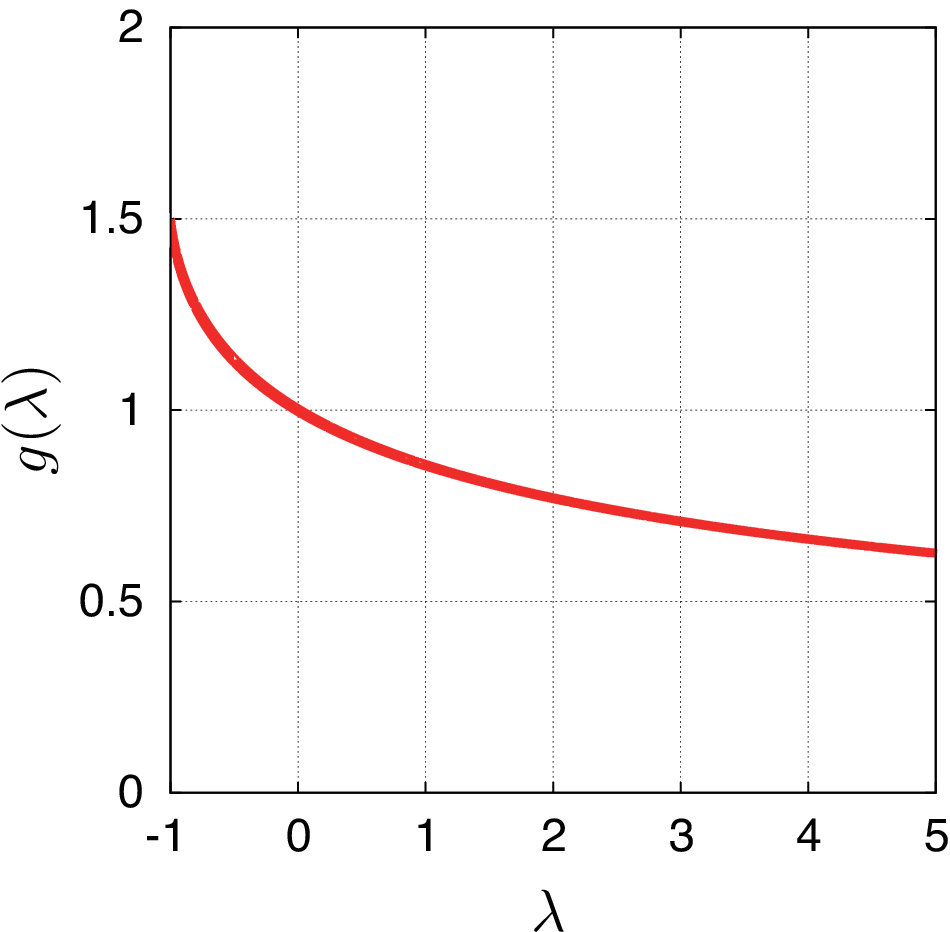
Figure 6: (Color online) The function g⁡(λ)g(\lambda) [Eq. 107], where λ\lambda is the ellipticity parameter of the ultraviolet cut-off [Eq. 65].

IV.3 Regularization dependence of Fermi-sea term

In cases (ii) and (iii), the Fermi-sea terms contain ultraviolet divergences and we have managed them by introducing a momemtum cut-off Λ\Lambda and letting Λ→∞\Lambda\to\infty at the end. The above results, Eq. 64 and first terms in Eqs. 60b and 60c, were obtained based on the isotropic cut-off, |𝒌|<Λ|{\bm{k}}|<\Lambda. If other cut-off scheme is used (such as the anisotropic one), one generally obtains a different value. For example, if we take the “elliptical” cut-off,

k⟂2+(1+λ)​kz2≤Λ2(−1<λ<∞),k_{\perp}^{2}+(1+\lambda)k_{z}^{2}\leq\Lambda^{2}\quad(-1<\lambda<\infty), (65)

Eq. 64 is replaced by

σx​y​(μ=0)=−α​S3​π2​ℏ​g​(λ),\sigma_{xy}(\mu=0)=-\frac{\alpha S}{3\pi^{2}\hbar}\,g(\lambda), (66)

[so are the first terms of Eqs. 60b and 60c], where g⁡(λ)g(\lambda) is given by Eq. 107 and plotted in Fig. 6. (See Appendices C and D for details). While the isotropic cut-off seems to be most natural, anisotropic cut-off may find its relevance in real materials having crystal anisotropy.

V Summary

We have proposed a model ferromagnet based on the Dirac Hamiltonian in 3D by noting that there are two possible ferromagnetic order parameters, 𝑴\bm{M} and 𝑺\bm{S}. By restricting ourselves to the case where 𝑴\bm{M} and 𝑺\bm{S} are collinear, we have studied its magneto-transport properties, which are AMR and AHE. The AMR is found to be determined primarily by the anisotropy of the Fermi surface (group velocity) and secondarily by the anisotropy of the damping. As for AHE, the present model offers an example of non-quantized Hall insulator state in which the Hall conductivity is proportional to 𝑺\bm{S} while the longitudinal conductivity vanishes. We have suggested that this may explain the peculiar property of Cr-doped (Bi,Sb)2Te3 found in a recent experiment.[10]

In this paper, we have restricted ourselves to the process represented by a simple bubble diagram, in which only the self-energy effects are considered. It will be important to study the effects of vertex corrections such as ladder and skew scattering. These will be reported in the future.

Note added: After submitting the manuscript, we got to know that the Fermi-sea term of the Hall conductivity was calculated by Burkov[36] in essentially the same model as our “𝑺\bm{S} model”. However, he obtained a vanishing Hall conductivity when the chemical potential lies in the gap, which apparently disagrees with our result. This discrepancy seems to originate from the difference in the “cut-off anisotropy” (in our terminology). Namely, Burkov considers a layered system of two-dimensional continuum planes, which may correspond to λ=∞\lambda=\infty in our model (see Eq. 65); in this special case of λ=∞\lambda=\infty, our calculation gives σx​y=0\sigma_{xy}=0 (see Fig. 6 or Eq. 107) in agreement with Burkov’s result. This seems to indicate that our “𝑺{\bm{S}} model” can be regarded as a continuum version of the Burkov’s model, and that this extension has a non-trivial consequence (Hall insulator state) due to the ultraviolet divergence. We would like to thank Anton Burkov for directing our attention to Ref. 36 and for subsequent informative discussions.

Acknowledgements.
The authors would like to thank Prof. N. Samarth for his kind correspondence. This work was supported by Grants-in-Aid for Scientific Research (No. 21540336, No. 24244053 and No. 25400339) from the Japan Society for the Promotion of Science (JSPS). JF is supported by JSPS Research Fellowship for Young Scientists.

Appendix A Damping constants

The damping constants γμ​ν​(ϵ)\gamma_{\mu\nu}(\epsilon) given by Eq. 15 are calculated as follows. Using the relation

Im​1D𝒌​(ϵ+i​0)=−π4​ϵ​(ϵ2−ϵk2)∑η,ζδ(ϵ−ζχ𝒌η(ϵ))=−π8​ϵ​Δ𝒌​(ϵ)∑η,ζηδ(ϵ−ζχ𝒌η(ϵ)),\begin{split}\mathrm{Im}\,\frac{1}{D_{\bm{k}}(\epsilon+i0)}&=-\frac{\pi}{4\epsilon(\epsilon^{2}-\epsilon_{k}^{2})}\sum_{\eta,\zeta}\delta(\epsilon-\zeta\chi_{\bm{k}}^{\eta}(\epsilon))\\ &=-\frac{\pi}{8\epsilon\Delta_{\bm{k}}(\epsilon)}\sum_{\eta,\zeta}\eta\delta(\epsilon-\zeta\chi_{\bm{k}}^{\eta}(\epsilon)),\end{split} (67)

where

χ𝒌η​(ϵ)=ϵk2+2​η​Δ𝒌​(ϵ),\chi_{\bm{k}}^{\eta}(\epsilon)=\sqrt{\epsilon_{k}^{2}+2\eta\Delta_{\bm{k}}(\epsilon)}, (68)

they are written as

γ00​(ϵ)\displaystyle\gamma_{00}(\epsilon) =π4​ni​u2​1ϵ​∑𝒌,η,ζ{ϵ−η​M​ΩΔ𝒌​(ϵ)}​δ​(ϵ−ζ​χ𝒌η​(ϵ)),\displaystyle=\frac{\pi}{4}n_{\mathrm{i}}u^{2}\frac{1}{\epsilon}\sum_{\bm{k},\eta,\zeta}\left\{\epsilon-\frac{\eta M\Omega}{\Delta_{\bm{k}}(\epsilon)}\right\}\delta(\epsilon-\zeta\chi_{\bm{k}}^{\eta}(\epsilon)), (69a)
γ30​(ϵ)\displaystyle\gamma_{30}(\epsilon) =π4​ni​u2​1ϵ​∑𝒌,η,ζ{m+η​S​ΩΔ𝒌​(ϵ)}​δ​(ϵ−ζ​χ𝒌η​(ϵ)),\displaystyle=\frac{\pi}{4}n_{\mathrm{i}}u^{2}\frac{1}{\epsilon}\sum_{\bm{k},\eta,\zeta}\left\{m+\frac{\eta S\Omega}{\Delta_{\bm{k}}(\epsilon)}\right\}\delta(\epsilon-\zeta\chi_{\bm{k}}^{\eta}(\epsilon)), (69b)
γ0​z​(ϵ)\displaystyle\gamma_{0z}(\epsilon) =−π4niu21ϵ∑𝒌,η,ζ{S+η​S​kz2Δ𝒌​(ϵ)+η​m​ΩΔ𝒌​(ϵ)}δ(ϵ−ζχ𝒌η(ϵ)),\displaystyle=-\frac{\pi}{4}n_{\mathrm{i}}u^{2}\frac{1}{\epsilon}\sum_{\bm{k},\eta,\zeta}\left\{S+\frac{\eta Sk_{z}^{2}}{\Delta_{\bm{k}}(\epsilon)}+\frac{\eta m\Omega}{\Delta_{\bm{k}}(\epsilon)}\right\}\delta(\epsilon-\zeta\chi_{\bm{k}}^{\eta}(\epsilon)), (69c)
γ3​z​(ϵ)\displaystyle\gamma_{3z}(\epsilon) =π4​ni​u2​1ϵ​∑𝒌,η,ζ{M+η​M​kz2Δ𝒌​(ϵ)−η​ϵ​ΩΔ𝒌​(ϵ)}​δ​(ϵ−ζ​χ𝒌η​(ϵ)).\displaystyle=\frac{\pi}{4}n_{\mathrm{i}}u^{2}\frac{1}{\epsilon}\sum_{\bm{k},\eta,\zeta}\left\{M+\frac{\eta Mk_{z}^{2}}{\Delta_{\bm{k}}(\epsilon)}-\frac{\eta\epsilon\Omega}{\Delta_{\bm{k}}(\epsilon)}\right\}\delta(\epsilon-\zeta\chi_{\bm{k}}^{\eta}(\epsilon)). (69d)

If we define

νl,mη​(ϵ)=∑𝒌,ζkz2​m[Δ𝒌​(ϵ)]l​δ​(ϵ−ζ​χ𝒌η​(ϵ)),\nu_{l,m}^{\eta}(\epsilon)=\sum_{\bm{k},\zeta}\frac{k_{z}^{2m}}{[\Delta_{\bm{k}}(\epsilon)]^{l}}\delta(\epsilon-\zeta\chi_{\bm{k}}^{\eta}(\epsilon)), (70)

the γμ​ν​(ϵ)\gamma_{\mu\nu}(\epsilon)’s are expressed as

γ00​(ϵ)\displaystyle\gamma_{00}(\epsilon) =π4​ni​u2​1ϵ​∑η(ϵ​ν0,0η​(ϵ)−η​M​Ω​ν1,0η​(ϵ)),\displaystyle=\frac{\pi}{4}n_{\mathrm{i}}u^{2}\frac{1}{\epsilon}\sum_{\eta}(\epsilon\nu_{0,0}^{\eta}(\epsilon)-\eta M\Omega\nu_{1,0}^{\eta}(\epsilon)), (71a)
γ30​(ϵ)\displaystyle\gamma_{30}(\epsilon) =π4​ni​u2​1ϵ​∑η(m​ν0,0η​(ϵ)+η​S​Ω​ν1,0η​(ϵ)),\displaystyle=\frac{\pi}{4}n_{\mathrm{i}}u^{2}\frac{1}{\epsilon}\sum_{\eta}(m\nu_{0,0}^{\eta}(\epsilon)+\eta S\Omega\nu_{1,0}^{\eta}(\epsilon)), (71b)
γ0​z​(ϵ)\displaystyle\gamma_{0z}(\epsilon) =−π4niu21ϵ∑η(Sν0,0η(ϵ)+ηSν1,1η(ϵ)+ηmΩν1,0η(ϵ)),\displaystyle=-\frac{\pi}{4}n_{\mathrm{i}}u^{2}\frac{1}{\epsilon}\sum_{\eta}(S\nu_{0,0}^{\eta}(\epsilon)+\eta S\nu_{1,1}^{\eta}(\epsilon)+\eta m\Omega\nu_{1,0}^{\eta}(\epsilon)), (71c)
γ3​z​(ϵ)\displaystyle\gamma_{3z}(\epsilon) =π4​ni​u2​1ϵ​∑η(M​ν0,0η​(ϵ)+η​M​ν1,1η​(ϵ)−η​ϵ​Ω​ν1,0η​(ϵ)).\displaystyle=\frac{\pi}{4}n_{\mathrm{i}}u^{2}\frac{1}{\epsilon}\sum_{\eta}(M\nu_{0,0}^{\eta}(\epsilon)+\eta M\nu_{1,1}^{\eta}(\epsilon)-\eta\epsilon\Omega\nu_{1,0}^{\eta}(\epsilon)). (71d)

For (l,m)=(0,0),(1,0),(1,1)(l,m)=(0,0),(1,0),(1,1), they are calculated as

ν0,0η​(ϵ)\displaystyle\nu_{0,0}^{\eta}(\epsilon) =|ϵ|2​π2​Θη​(ϵ)​ξη​(ϵ),\displaystyle=\frac{|\epsilon|}{2\pi^{2}}\Theta_{\eta}(\epsilon)\xi_{\eta}(\epsilon), (72)
ν1,0η​(ϵ)\displaystyle\nu_{1,0}^{\eta}(\epsilon) =|ϵ|2​π2​Θη​(ϵ)​hη​(ϵ),\displaystyle=\frac{|\epsilon|}{2\pi^{2}}\Theta_{\eta}(\epsilon)h_{\eta}(\epsilon), (73)
ν1,1η​(ϵ)\displaystyle\nu_{1,1}^{\eta}(\epsilon) =|ϵ|4​π2​Θη​(ϵ)​1S2−M2​(ξη​(ϵ)​Ω2+(S2−M2)​[ξη​(ϵ)]2−Ω2​hη​(ϵ)),\displaystyle=\frac{|\epsilon|}{4\pi^{2}}\Theta_{\eta}(\epsilon)\frac{1}{S^{2}-M^{2}}\left(\xi_{\eta}(\epsilon)\sqrt{\Omega^{2}+(S^{2}-M^{2})[\xi_{\eta}(\epsilon)]^{2}}-\Omega^{2}h_{\eta}(\epsilon)\right), (74)

where

hη​(ϵ)={1S2−M2​tanh−1⁡ξη​(ϵ)​S2−M2Ω2+(S2−M2)​[ξη​(ϵ)]2(S2−M2>0),1|S2−M2|​tan−1⁡ξη​(ϵ)​|S2−M2|Ω2−|S2−M2|​[ξη​(ϵ)]2(S2−M2<0),h_{\eta}(\epsilon)=\left\{\begin{array}[]{c c}\displaystyle\frac{1}{\sqrt{S^{2}-M^{2}}}\tanh^{-1}\frac{\xi_{\eta}(\epsilon)\sqrt{S^{2}-M^{2}}}{\sqrt{\Omega^{2}+(S^{2}-M^{2})[\xi_{\eta}(\epsilon)]^{2}}}&\ \ \ (S^{2}-M^{2}>0),\\ \displaystyle\frac{1}{\sqrt{|S^{2}-M^{2}|}}\tan^{-1}\frac{\xi_{\eta}(\epsilon)\sqrt{|S^{2}-M^{2}|}}{\sqrt{\Omega^{2}-|S^{2}-M^{2}|[\xi_{\eta}(\epsilon)]^{2}}}&\ \ \ (S^{2}-M^{2}<0),\end{array}\right. (75)

and ξη​(ϵ)\xi_{\eta}(\epsilon) and Θη​(ϵ)\Theta_{\eta}(\epsilon) are defined by Eqs. 49 and 44, respectively.

Appendix B “Magnetization” model

In this Appendix, we show some details of the calculation for the “magnetization” model, in which 𝑴=M​z^\bm{M}=M\hat{z} and 𝑺=0\bm{S}=0 [case (i)]. The denominator, D𝒌​(ϵ)D_{\bm{k}}(\epsilon), of the unperturbed Green’s function is given by

D𝒌​(ϵ)\displaystyle D_{\bm{k}}(\epsilon) =(ϵ−E𝒌+)​(ϵ+E𝒌+)​(ϵ−E𝒌−)​(ϵ+E𝒌−),\displaystyle=(\epsilon-E_{\bm{k}}^{+})(\epsilon+E_{\bm{k}}^{+})(\epsilon-E_{\bm{k}}^{-})(\epsilon+E_{\bm{k}}^{-}),\hskip 17.22217pt (76)
E𝒌η\displaystyle E_{\bm{k}}^{\eta} =k2+m2+M2+2​η​M​k⟂2+m2\displaystyle=\sqrt{k^{2}+m^{2}+M^{2}+2\eta M\sqrt{k^{2}_{\perp}+m^{2}}} (77)
=ϵk2+2​M2+2​η​M​k⟂2+m2,\displaystyle=\sqrt{\epsilon_{k}^{2}+2M^{2}+2\eta M\sqrt{k^{2}_{\perp}+m^{2}}}, (78)

where η=±\eta=\pm, k⟂2=kx2+ky2k_{\perp}^{2}=k_{x}^{2}+k_{y}^{2}, and ϵk2=k2+m2−M2\epsilon_{k}^{2}=k^{2}+m^{2}-M^{2}.

It is convenient to define the generalized density of states by

𝒩l,η​(ϵ)=∑𝒌∑ζ=±1(k⟂2+m2)l/2​δ​(ϵ−ζ​E𝒌η).\mathcal{N}_{l,\eta}(\epsilon)=\sum_{\bm{k}}\sum_{\zeta=\pm 1}(k_{\perp}^{2}+m^{2})^{l/2}\delta(\epsilon-\zeta E_{\bm{k}}^{\eta}). (79)

Using the relation ∑ζδ⁡(ϵ−ζ​E𝒌η)=2​|ϵ|​δ​(kz2−ϵ2+(k⟂2+m2+η​M)2)\sum_{\zeta}\delta(\epsilon-\zeta E_{\bm{k}}^{\eta})=2|\epsilon|\delta(k_{z}^{2}-\epsilon^{2}+(\sqrt{k_{\perp}^{2}+m^{2}}+\eta M)^{2}) and performing the 𝒌\bm{k}-integration, those of our interest (see below) are obtained as

𝒩−1,η​(ϵ)\displaystyle\mathcal{N}_{-1,\eta}(\epsilon) =|ϵ|2​π2​Θη​(ϵ)​(π2−ψa),\displaystyle=\frac{|\epsilon|}{2\pi^{2}}\Theta_{\eta}(\epsilon)\left(\frac{\pi}{2}-\psi_{a}\right), (80)
𝒩0,η​(ϵ)\displaystyle\mathcal{N}_{0,\eta}(\epsilon) =|ϵ|2​π2Θη(ϵ)(|ϵ|cosψa−ηM(π2−ψa)),\displaystyle=\frac{|\epsilon|}{2\pi^{2}}\Theta_{\eta}(\epsilon)\left(|\epsilon|\cos\psi_{a}-\eta M\left(\frac{\pi}{2}-\psi_{a}\right)\right), (81)
𝒩1,η​(ϵ)\displaystyle\mathcal{N}_{1,\eta}(\epsilon) =|ϵ|4​π2Θη(ϵ)((m−3ηM)|ϵ|cosψa+(ϵ2+2M2)(π2−ψa)),\displaystyle=\frac{|\epsilon|}{4\pi^{2}}\Theta_{\eta}(\epsilon)\left((m-3\eta M)|\epsilon|\cos\psi_{a}+(\epsilon^{2}+2M^{2})\left(\frac{\pi}{2}-\psi_{a}\right)\right), (82)

where ψa=sin−1⁡[(m+η​M)/|ϵ|]\psi_{a}=\sin^{-1}[(m+\eta M)/|\epsilon|], and

Θη​(ϵ)={1(|ϵ|>m+η​M)0(otherwise).\Theta_{\eta}(\epsilon)=\left\{\begin{array}[]{c c}1&\quad(|\epsilon|>m+\eta M)\\ 0&\quad(\text{otherwise}).\end{array}\right. (83)

To calculate σx​y(3)\sigma^{(3)}_{xy}, we note X⁡(ϵ)=−4​m​M​ϵ​(ϵ2−ϵk2)X(\epsilon)=-4mM\epsilon\left(\epsilon^{2}-\epsilon_{k}^{2}\right) [Eq. 58] and ∂ϵD𝒌=4​ϵ​(ϵ2−ϵk2−2​M2)\partial_{\epsilon}D_{\bm{k}}=4\epsilon(\epsilon^{2}-\epsilon_{k}^{2}-2M^{2}), and rewrite Eq. 59 as

σx​y(3)=−m​e22​μ∑η(η𝒩−1,η(μ)+M𝒩−2,η(μ))−m​e22∑ηη∑𝒌,ζ1(k⟂2+m2)3/2∫−∞μdϵδ(ϵ−ζE𝒌η).\sigma_{xy}^{(3)}=-\frac{me^{2}}{2\mu}\sum_{\eta}\left(\eta\mathcal{N}_{-1,\eta}(\mu)+M\mathcal{N}_{-2,\eta}(\mu)\right)-\frac{me^{2}}{2}\sum_{\eta}\eta\sum_{\bm{k},\zeta}\frac{1}{(k_{\perp}^{2}+m^{2})^{3/2}}\int_{-\infty}^{\mu}d\epsilon\,\delta(\epsilon-\zeta E_{\bm{k}}^{\eta}). (84)

In the second term on the right-hand side, the ϵ\epsilon-integral in the range (−∞,0)(-\infty,0) vanishes because of ∑ηη\sum_{\eta}\eta = 0, and the rest of the ϵ\epsilon- and 𝒌\bm{k}-integrals are calculated as follows:

∑𝒌,ζ1(k⟂2+m2)3/2​∫0μd​ϵ​δ​(ϵ−ζ​E𝒌η)=1(2​π)2​Θη​(μ)​∫0ξηd​k⟂​2​k⟂(k⟂2+m2)3/2​∫0μ2−(k⟂2+m2+η​M)2d​kz=μ​|μ|2​π2​Θη​(μ)​∫ψaψbd​θ​cos2⁡θ(μ​sin⁡θ−η​M)2=|μ|2​π2Θη(μ)[1mcosψa−1μ∫ψaψbdθ(1+η​Mμ​sin⁡θ−η​M)]=1m​μ​(𝒩0,η​(μ)+η​M​𝒩−1,η​(μ))−1μ​(𝒩−1,η​(μ)+η​M​𝒩−2,η​(μ)).\begin{split}\sum_{\bm{k},\zeta}\frac{1}{(k_{\perp}^{2}+m^{2})^{3/2}}\int_{0}^{\mu}d\epsilon\,\delta(\epsilon-\zeta E_{\bm{k}}^{\eta})&=\frac{1}{(2\pi)^{2}}\Theta_{\eta}(\mu)\int_{0}^{\xi_{\eta}}dk_{\perp}\,\frac{2k_{\perp}}{(k_{\perp}^{2}+m^{2})^{3/2}}\int_{0}^{\sqrt{\mu^{2}-\left(\sqrt{k_{\perp}^{2}+m^{2}}+\eta M\right)^{2}}}dk_{z}\,\\ &=\frac{\mu|\mu|}{2\pi^{2}}\Theta_{\eta}(\mu)\int_{\psi_{a}}^{\psi_{b}}d\theta\,\frac{\cos^{2}\theta}{(\mu\sin\theta-\eta M)^{2}}\\ &=\frac{|\mu|}{2\pi^{2}}\Theta_{\eta}(\mu)\left[\frac{1}{m}\cos\psi_{a}-\frac{1}{\mu}\int_{\psi_{a}}^{\psi_{b}}d\theta\,\left(1+\frac{\eta M}{\mu\sin\theta-\eta M}\right)\right]\\ &=\frac{1}{m\mu}\left(\mathcal{N}_{0,\eta}(\mu)+\eta M\mathcal{N}_{-1,\eta}(\mu)\right)-\frac{1}{\mu}(\mathcal{N}_{-1,\eta}(\mu)+\eta M\mathcal{N}_{-2,\eta}(\mu)).\end{split} (85)

Therefore, the second term in Eq. 84 can be rewritten as

−e22​μ∑η[(η𝒩0,η(μ)+M𝒩−1,η(μ))−m(η𝒩−1,η(μ)+M𝒩−2,η(μ))],-\frac{e^{2}}{2\mu}\sum_{\eta}\left[\left(\eta\mathcal{N}_{0,\eta}(\mu)+M\mathcal{N}_{-1,\eta}(\mu)\right)-m(\eta\mathcal{N}_{-1,\eta}(\mu)+M\mathcal{N}_{-2,\eta}(\mu))\right], (86)

and we obtain

σx​y(3)=−e22​μ∑η(η𝒩0,η(μ)+M𝒩−1,η(μ))=−sign(μ)e24​π2∑ηηΘη(μ)μ2−(m+η​M)2.\begin{split}\sigma_{xy}^{(3)}&=-\frac{e^{2}}{2\mu}\sum_{\eta}\left(\eta\mathcal{N}_{0,\eta}(\mu)+M\mathcal{N}_{-1,\eta}(\mu)\right)\\ &=-\mathrm{sign}(\mu)\,\frac{e^{2}}{4\pi^{2}}\sum_{\eta}\eta\,\Theta_{\eta}(\mu)\sqrt{\mu^{2}-(m+\eta M)^{2}}.\end{split} (87)

These are shown in Fig. 5 (i) as the Fermi-sea term.

Appendix C “Spin” model

For the “spin” model, where 𝑴=0\bm{M}=0 and 𝑺=S​z^\bm{S}=S\hat{z} [case (ii)], the denominator D𝒌​(ϵ)D_{\bm{k}}(\epsilon) [Eq. 9] of the unperturbed Green’s function is given by

D𝒌​(ϵ)\displaystyle D_{\bm{k}}(\epsilon) =(ϵ−E𝒌+)​(ϵ+E𝒌+)​(ϵ−E𝒌−)​(ϵ+E𝒌−),\displaystyle=(\epsilon-E_{\bm{k}}^{+})(\epsilon+E_{\bm{k}}^{+})(\epsilon-E_{\bm{k}}^{-})(\epsilon+E_{\bm{k}}^{-}), (88)
E𝒌η\displaystyle E_{\bm{k}}^{\eta} =k2+m2+S2+2​η​S​kz2+m2\displaystyle=\sqrt{k^{2}+m^{2}+S^{2}+2\eta S\sqrt{k^{2}_{z}+m^{2}}} (89)
=ϵk2+2​η​S​kz2+m2,\displaystyle=\sqrt{\epsilon_{k}^{2}+2\eta S\sqrt{k^{2}_{z}+m^{2}}}, (90)

where ϵk2=k2+m2+S2\epsilon_{k}^{2}=k^{2}+m^{2}+S^{2}.

The generalized density of states in this case is defined by

𝒩l,η​(ϵ)=∑𝒌,ζ(kz2+m2)l/2​δ​(ϵ−ζ​E𝒌η),\mathcal{N}_{l,\eta}(\epsilon)=\sum_{\bm{k},\zeta}(k_{z}^{2}+m^{2})^{l/2}\delta(\epsilon-\zeta E_{\bm{k}}^{\eta}), (91)

some of which are calculated as

𝒩−1,η​(ϵ)\displaystyle\mathcal{N}_{-1,\eta}(\epsilon) =|ϵ|2​π2​θη∗​(ϵ)​Θη​(ϵ),\displaystyle=\frac{|\epsilon|}{2\pi^{2}}\theta_{\eta}^{*}(\epsilon)\Theta_{\eta}(\epsilon), (92)
𝒩0,η​(ϵ)\displaystyle\mathcal{N}_{0,\eta}(\epsilon) =m​|ϵ|2​π2sinhθη∗(ϵ)Θη(ϵ),\displaystyle=\frac{m|\epsilon|}{2\pi^{2}}\sinh\theta_{\eta}^{*}(\epsilon)\Theta_{\eta}(\epsilon), (93)
𝒩1,η​(ϵ)\displaystyle\mathcal{N}_{1,\eta}(\epsilon) =m2​|ϵ|4​π2(θη∗+sinhθη∗(ϵ)coshθη∗(ϵ))Θη(ϵ),\displaystyle=\frac{m^{2}|\epsilon|}{4\pi^{2}}\left(\theta_{\eta}^{*}+\sinh\theta_{\eta}^{*}(\epsilon)\cosh\theta_{\eta}^{*}(\epsilon)\right)\Theta_{\eta}(\epsilon), (94)

where θη∗​(ϵ)=cosh−1⁡[(|ϵ|−η​S)/m]\theta_{\eta}^{*}(\epsilon)=\cosh^{-1}[(|\epsilon|-\eta S)/m] and

Θη​(ϵ)={1(|ϵ|>m+η​S)0(otherwise).\Theta_{\eta}(\epsilon)=\left\{\begin{array}[]{c c}1&\quad(|\epsilon|>m+\eta S)\\ 0&\quad(\text{otherwise}).\end{array}\right. (95)

To calculate σx​y(3)\sigma^{(3)}_{xy}, we first express it as

σx​y(3)=−e22​μ2∑η(S𝒩0,η(μ)+η𝒩1,η(μ))−e22∑𝒌,η,ζηkz2+m2+η​Sζ​(E𝒌η)3∫−∞μdϵδ(ϵ−ζE𝒌η),\sigma_{xy}^{(3)}=-\frac{e^{2}}{2\mu^{2}}\sum_{\eta}\left(S\mathcal{N}_{0,\eta}(\mu)+\eta\mathcal{N}_{1,\eta}(\mu)\right)-\frac{e^{2}}{2}\sum_{\bm{k},\eta,\zeta}\eta\frac{\sqrt{k_{z}^{2}+m^{2}}+\eta S}{\zeta\left(E_{\bm{k}}^{\eta}\right)^{3}}\int_{-\infty}^{\mu}d\epsilon\,\delta(\epsilon-\zeta E_{\bm{k}}^{\eta}), (96)

by noting that X⁡(ϵ)=−S⁡{Dk+4​(kz2+m2)​(ϵ2−ϵk2+2​S2)}X(\epsilon)=-S\{D_{k}+4(k_{z}^{2}+m^{2})(\epsilon^{2}-\epsilon_{k}^{2}+2S^{2})\} and ∂ϵDk=4​ϵ​(ϵ2−ϵk2)\partial_{\epsilon}D_{k}=4\epsilon(\epsilon^{2}-\epsilon_{k}^{2}). In the second term on the right-hand side, the ϵ\epsilon-integral in the range (−∞,0)(-\infty,0) is calculated as

−e22∑𝒌,η,ζηkz2+m2+η​Sζ​(E𝒌η)3∫−∞0dϵδ(ϵ−ζE𝒌η)=e22∑𝒌,ηS+η​kz2+m2(E𝒌η)3.-\frac{e^{2}}{2}\sum_{\bm{k},\eta,\zeta}\eta\frac{\sqrt{k_{z}^{2}+m^{2}}+\eta S}{\zeta\left(E_{\bm{k}}^{\eta}\right)^{3}}\int_{-\infty}^{0}d\epsilon\,\delta(\epsilon-\zeta E_{\bm{k}}^{\eta})=\frac{e^{2}}{2}\sum_{\bm{k},\eta}\frac{S+\eta\sqrt{k_{z}^{2}+m^{2}}}{\left(E_{\bm{k}}^{\eta}\right)^{3}}. (97)

In calculating this 𝒌\bm{k}-integral, a care is needed since it is ultraviolet divergent. To manage this divergence, we introduce a momentum cut-off Λ\Lambda and limit the integration to a spherical region, |𝒌|<Λ|{\bm{k}}|<\Lambda, and then let Λ→∞\Lambda\to\infty. This proceeds as follows; we first write

e22​(2​π)2​limΛ→∞∑η∫0Λd​kz​(S+η​kz2+m2)​∫0Λ2−kz2d​k⟂​ 2​k⟂​(1k⟂2+(S+η​kz2+m2)2)3/2=−e2(2​π)2limΛ→∞∑η∫0ΛdkzS+η​kz2+m2Λ2−kz2+(S+η​kz2+m2)2,\begin{split}&\frac{e^{2}}{2(2\pi)^{2}}\lim_{\Lambda\to\infty}\sum_{\eta}\int_{0}^{\Lambda}dk_{z}\,(S+\eta\sqrt{k_{z}^{2}+m^{2}})\int_{0}^{\sqrt{\Lambda^{2}-k_{z}^{2}}}dk_{\perp}\,2k_{\perp}\left(\frac{1}{k_{\perp}^{2}+(S+\eta\sqrt{k_{z}^{2}+m^{2}})^{2}}\right)^{3/2}\\ &=-\frac{e^{2}}{(2\pi)^{2}}\lim_{\Lambda\to\infty}\sum_{\eta}\int_{0}^{\Lambda}dk_{z}\,\frac{S+\eta\sqrt{k_{z}^{2}+m^{2}}}{\sqrt{\Lambda^{2}-k_{z}^{2}+\left(S+\eta\sqrt{k_{z}^{2}+m^{2}}\right)^{2}}},\end{split} (98)

then scale as kz=Λ​t,m~=m/Λ,S~=S/Λk_{z}=\Lambda t,\tilde{m}=m/\Lambda,\tilde{S}=S/\Lambda, and sum over η\eta. The result is the left-hand side of

−S​e2(2​π)2limΛ→∞∫01dt{𝒜(t)−4ℬ(t)}=−S​e23​π2,-\frac{Se^{2}}{(2\pi)^{2}}\lim_{\Lambda\to\infty}\int_{0}^{1}dt\,\left\{\mathcal{A}(t)-4\mathcal{B}(t)\right\}=-\frac{Se^{2}}{3\pi^{2}}, (99)

with

𝒜⁡(t)\displaystyle\mathcal{A}(t) =∑η{1−t2+(S~+ηt2+m~2)2}−1/2,\displaystyle=\sum_{\eta}\left\{1-t^{2}+\left(\tilde{S}+\eta\sqrt{t^{2}+\tilde{m}^{2}}\right)^{2}\right\}^{-1/2}, (100)
ℬ⁡(t)\displaystyle\mathcal{B}(t) =t2+m~2∑η{1−t2+(S~+η​t2+m~2)2}1/2​∏η′{1−t2+(S~+η′​t2+m~2)2}1/2.\displaystyle=\frac{t^{2}+\tilde{m}^{2}}{\displaystyle\sum_{\eta}\left\{1-t^{2}+\left(\tilde{S}+\eta\sqrt{t^{2}+\tilde{m}^{2}}\right)^{2}\right\}^{1/2}\displaystyle\prod_{\eta^{\prime}}\left\{1-t^{2}+\left(\tilde{S}+\eta^{\prime}\sqrt{t^{2}+\tilde{m}^{2}}\right)^{2}\right\}^{1/2}}. (101)

We then let Λ→∞\Lambda\to\infty, thus S~→0,m~→0\tilde{S}\to 0,\tilde{m}\to 0, 𝒜→2\mathcal{A}\to 2 and ℬ→t2/2\mathcal{B}\to t^{2}/2, and integrate over tt; this leads to the right-hand side of Eq. 99. The rest of the integral, which is divergence-free, is calculated as follows,

−e22​(2​π)2∑ηΘη(μ)∫0ξηdkz(S+ηkz2+m2)∫0αηdt(1t+(S+η​kz2+m2)2)3/2=e22​|μ|​12​π2​∑ηΘη​(μ)​∫0ξηd​kz​(S−η​|μ|+η​kz2+m2)=e22​|μ|​12​π2​∑ηΘη​(μ)​∫0θη∗d​θ​m​cosh⁡θ⁡(S−η​|μ|+η​m​cosh⁡θ)=e22​μ2​∑η{(S−η​|μ|)​𝒩0,η​(μ)+η​𝒩1,η​(μ)}.\begin{split}&-\frac{e^{2}}{2(2\pi)^{2}}\sum_{\eta}\Theta_{\eta}(\mu)\int_{0}^{\xi_{\eta}}dk_{z}\,(S+\eta\sqrt{k_{z}^{2}+m^{2}})\int_{0}^{\alpha_{\eta}}dt\,\left(\frac{1}{t+(S+\eta\sqrt{k_{z}^{2}+m^{2}})^{2}}\right)^{3/2}\\ &=\frac{e^{2}}{2|\mu|}\frac{1}{2\pi^{2}}\sum_{\eta}\Theta_{\eta}(\mu)\int_{0}^{\xi_{\eta}}dk_{z}\,\left(S-\eta|\mu|+\eta\sqrt{k_{z}^{2}+m^{2}}\right)\\ &=\frac{e^{2}}{2|\mu|}\frac{1}{2\pi^{2}}\sum_{\eta}\Theta_{\eta}(\mu)\int_{0}^{\theta^{*}_{\eta}}d\theta\,m\cosh\theta\left(S-\eta|\mu|+\eta m\cosh\theta\right)\\ &=\frac{e^{2}}{2\mu^{2}}\sum_{\eta}\left\{(S-\eta|\mu|)\mathcal{N}_{0,\eta}(\mu)+\eta\mathcal{N}_{1,\eta}(\mu)\right\}.\end{split} (102)

Therefore we obtain

σx​y(3)=−S​e23​π2−e22​|μ|​∑ηη​𝒩0,η​(μ)=−S​e23​π2−e24​π2​∑ηη​Θη​(μ)​(|μ|−η​S)2−m2.\begin{split}\sigma_{xy}^{(3)}&=-\frac{Se^{2}}{3\pi^{2}}-\frac{e^{2}}{2|\mu|}\sum_{\eta}\eta\mathcal{N}_{0,\eta}(\mu)\\ &=-\frac{Se^{2}}{3\pi^{2}}-\frac{e^{2}}{4\pi^{2}}\sum_{\eta}\eta\Theta_{\eta}(\mu)\sqrt{(|\mu|-\eta S)^{2}-m^{2}}.\end{split} (103)

This is plotted in Fig. 5 (ii) as the Fermi-sea term. The first term corresponds to σx​y​(μ=0)\sigma_{xy}(\mu=0).

It should be noted that, if another cut-off scheme is adopted, one would obtain a different result in general. For example, if we introduce two cut-off parameters, Λ⟂\Lambda_{\perp} and Λz\Lambda_{z}, limit the integration to a cylindrical region, |𝒌⟂|<Λ⟂|{\bm{k}}_{\perp}|<\Lambda_{\perp} and |kz|<Λz|k_{z}|<\Lambda_{z}, and let Λ⟂→∞\Lambda_{\perp}\to\infty and Λz→∞\Lambda_{z}\to\infty by keeping the ratio Λ⟂/Λz≡r\Lambda_{\perp}/\Lambda_{z}\equiv r constant, the first term of Eq. 103 is replaced by

σx​y​(μ=0)=−S​e22​π2​r2+1.\sigma_{xy}(\mu=0)=-\frac{Se^{2}}{2\pi^{2}\sqrt{r^{2}+1}}. (104)

Another, probably more natural cut-off which allows anisotropy would be an “elliptical” cut-off [Eq. 65],

k⟂2+(1+λ)​kz2≤Λ2,(−1<λ<∞).k_{\perp}^{2}+(1+\lambda)k_{z}^{2}\leq\Lambda^{2},\qquad(-1<\lambda<\infty). (105)

In this case, the first term of Eq. 103 is replaced by

σx​y​(μ=0)=−S​e23​π2​g​(λ),\sigma_{xy}(\mu=0)=-\frac{Se^{2}}{3\pi^{2}}\,g(\lambda), (106)

where

g⁡(λ)={32​λ​[(1+λ)​tanh−1⁡−λ−λ−1](−1<λ<0),32​λ​[(1+λ)​tan−1⁡λλ−1](λ>0),g(\lambda)=\left\{\begin{array}[]{c c}\displaystyle\frac{3}{2\lambda}\left[(1+\lambda)\frac{\tanh^{-1}\sqrt{-\lambda}}{\sqrt{-\lambda}}-1\,\right]&\qquad(-1<\lambda<0),\\ \displaystyle\frac{3}{2\lambda}\left[(1+\lambda)\frac{\tan^{-1}\sqrt{\lambda}}{\sqrt{\lambda}}-1\,\right]&\qquad(\lambda>0),\end{array}\right. (107)

which is plotted in Fig. 6. The value g⁡(−1)=3/2g(-1)=3/2 at λ=−1\lambda=-1 is consistent with Eq. 104 with r=0r=0.

Appendix D Coexistent’ Model

For the “coexistent” model with 𝑴=𝑺=S​z^\bm{M}=\bm{S}=S\hat{z} [case (iii)], the denominator D𝒌​(ϵ)D_{\bm{k}}(\epsilon) [Eq. 9] of the Green’s function is given by

Dk​(ϵ)\displaystyle D_{k}(\epsilon) =(ϵ−S−Ek+)​(ϵ+S−Ek+)​(ϵ−S+Ek−)​(ϵ+S+Ek−)\displaystyle=(\epsilon-S-E_{k}^{+})(\epsilon+S-E_{k}^{+})(\epsilon-S+E_{k}^{-})(\epsilon+S+E_{k}^{-}) (108)
=∏η,ζ=±(ϵ−ηS−ζEkη),\displaystyle=\prod_{\eta,\zeta=\pm}(\epsilon-\eta S-\zeta E_{k}^{\eta}), (109)
Ekη\displaystyle E_{k}^{\eta} =k2+(m+η​S)2.\displaystyle=\sqrt{k^{2}+(m+\eta S)^{2}}. (110)

In this case, the electron dispersion ϵ=η​S+ζ​Ekη\epsilon=\eta S+\zeta E_{k}^{\eta} is isotropic but there is a loss of particle-hole symmetry, in contrast to the cases (i) and (ii).

The generalized density of states is defined by

𝒩n,lη​(ϵ)≡∑𝒌∑ζ(k⟂2−kz2)l(ϵ2−ϵk2)n​δ​(ϵ−η​S−ζ​Ekη)=∑𝒌∑ζ(k2/3)l(ϵ2−ϵk2)n​δ​(ϵ−η​S−ζ​Ekη),(l=0,1).\begin{split}\mathcal{N}_{n,l}^{\eta}(\epsilon)&\equiv\sum_{\bm{k}}\sum_{\zeta}\frac{(k_{\perp}^{2}-k_{z}^{2})^{l}}{(\epsilon^{2}-\epsilon_{k}^{2})^{n}}\delta(\epsilon-\eta S-\zeta E_{k}^{\eta})\\ &=\sum_{\bm{k}}\sum_{\zeta}\frac{(k^{2}/3)^{l}}{(\epsilon^{2}-\epsilon_{k}^{2})^{n}}\delta(\epsilon-\eta S-\zeta E_{k}^{\eta}),\quad\quad(l=0,1).\end{split} (111)

In the second equality, which holds for l=0l=0 and 1, we have noted that the energy dispersion is isotropic. Explicitly, they are evaluated as

𝒩n,lη​(ϵ)=12​π2​13l​|ϵ−η​S|{2​η​S​(ϵ+m)}n​ξη2​l+1​Θη​(ϵ),(l=0,1),\begin{split}\mathcal{N}_{n,l}^{\eta}(\epsilon)&=\frac{1}{2\pi^{2}}\frac{1}{3^{l}}\frac{|\epsilon-\eta S|}{\{2\eta S(\epsilon+m)\}^{n}}\xi_{\eta}^{2l+1}\Theta_{\eta}(\epsilon),\qquad(l=0,1),\end{split} (112)

with ξη=(ϵ+m)​(ϵ−m−2​η​S)\xi_{\eta}=\sqrt{(\epsilon+m)(\epsilon-m-2\eta S)} and

Θη​(ϵ)={1(ϵ<−m,ϵ>m+2​η​S)0(otherwise).\Theta_{\eta}(\epsilon)=\left\{\begin{array}[]{c c}1&\qquad(\epsilon<-m,\,\epsilon>m+2\eta S)\\ 0&\qquad(\text{otherwise}).\end{array}\right. (113)

To calculate σx​y(3)\sigma^{(3)}_{xy}, we note X⁡(ϵ)=S​Dk−2​S​(ϵ2−ϵk2)​{(ϵ+m)2−k2+2​kz2}X(\epsilon)=SD_{k}-2S(\epsilon^{2}-\epsilon_{k}^{2})\{(\epsilon+m)^{2}-k^{2}+2k_{z}^{2}\} and ∂ϵDk=4​{ϵ⁡(ϵ2−ϵk2)−2​S2​(ϵ+m)}\partial_{\epsilon}D_{k}=4\{\epsilon(\epsilon^{2}-\epsilon_{k}^{2})-2S^{2}(\epsilon+m)\}, and express it as

σx​y(3)=−e26∑ημ+2​m+η​S(μ−η​S)2η𝒩η0,0(μ)−e22∑𝒌,η,ζηk2[(m+ηS)(k⟂2−2​kz2)(ζ​Ekη)3−2​kz2k2(m+η​Sζ​Ekη)3+2​kz2k2]∫−∞μdϵδ(ϵ−ηS−ζEkη),\begin{split}\sigma_{xy}^{(3)}&=-\frac{e^{2}}{6}\sum_{\eta}\frac{\mu+2m+\eta S}{(\mu-\eta S)^{2}}\eta\mathcal{N}^{\eta}_{0,0}(\mu)\\ &\hskip 10.00002pt-\frac{e^{2}}{2}\sum_{\bm{k},\eta,\zeta}\frac{\eta}{k^{2}}\left[(m+\eta S)\frac{(k_{\perp}^{2}-2k_{z}^{2})}{(\zeta E_{k}^{\eta})^{3}}-\frac{2k_{z}^{2}}{k^{2}}\left(\frac{m+\eta S}{\zeta E_{k}^{\eta}}\right)^{3}+\frac{2k_{z}^{2}}{k^{2}}\right]\int_{-\infty}^{\mu}d\epsilon\,\delta(\epsilon-\eta S-\zeta E_{k}^{\eta}),\end{split} (114)

where we used

∂ϵDk\displaystyle\partial_{\epsilon}D_{k} =8​η​ζ​S​Ekη​(ϵ+m),\displaystyle=8\eta\zeta SE_{k}^{\eta}(\epsilon+m), (115)
ϵ2−ϵk2\displaystyle\epsilon^{2}-\epsilon_{k}^{2} =2​η​S​(ϵ+m),\displaystyle=2\eta S(\epsilon+m), (116)
1ϵ+m\displaystyle\frac{1}{\epsilon+m} =−1k2​(ϵ+m−2​ζ​Ekη),\displaystyle=-\frac{1}{k^{2}}(\epsilon+m-2\zeta E_{k}^{\eta}), (117)

which hold under the presence of δ⁡(ϵ−η​S−ζ​Ekη)\delta(\epsilon-\eta S-\zeta E_{k}^{\eta}). In the second term on the right-hand side of Eq. 114, the ϵ\epsilon-integral from the range (−∞,0)(-\infty,0) is divided into the convergent part (𝒲0\mathcal{W}_{0}) and the conditionally-convergent part (𝒲1\mathcal{W}_{1}) due to ultraviolet divergence. They are respectively evaluated as follows; For 𝒲0\mathcal{W}_{0},

𝒲0≡−e22∑𝒌,η,ζηk2[−2​kz2k2(m+η​Sζ​Ekη)3+2​kz2k2]∫−∞0dϵδ(ϵ−ηS−ζEkη)=−e23∑𝒌,ηηk2(m+η​S)3(Ekη)3=−e2312​π2∑ηη∫0∞dk(m+η​S)3(Ekη)3=−S​e23​π2.\begin{split}\mathcal{W}_{0}&\equiv-\frac{e^{2}}{2}\sum_{\bm{k},\eta,\zeta}\frac{\eta}{k^{2}}\left[-\frac{2k_{z}^{2}}{k^{2}}\left(\frac{m+\eta S}{\zeta E_{k}^{\eta}}\right)^{3}+\frac{2k_{z}^{2}}{k^{2}}\right]\int_{-\infty}^{0}d\epsilon\,\delta(\epsilon-\eta S-\zeta E_{k}^{\eta})\\ &=-\frac{e^{2}}{3}\sum_{\bm{k},\eta}\frac{\eta}{k^{2}}\frac{(m+\eta S)^{3}}{\left(E_{k}^{\eta}\right)^{3}}\\ &=-\frac{e^{2}}{3}\frac{1}{2\pi^{2}}\sum_{\eta}\eta\int_{0}^{\infty}dk\,\frac{(m+\eta S)^{3}}{\left(E_{k}^{\eta}\right)^{3}}\\ &=-\frac{Se^{2}}{3\pi^{2}}.\end{split} (118)

For 𝒲1\mathcal{W}_{1}, we introduce a cut-off as k⟂2+(1+λ)​kz2≤Λ2k_{\perp}^{2}+(1+\lambda)k_{z}^{2}\leq\Lambda^{2} [Eq. 65 or Eq. 105], and evaluate as

𝒲1≡−e22∑𝒌,η,ζη​ζ(Ekη)31k2(m+ηS)(k⟂2−2kz2)∫−∞0dϵδ(ϵ−ηS−ζEkη)=limΛ→∞e22​(2​π)2​∑ηη⁡(m+η​S)​∫01/1+λd​q​∫q21−λ​q2d​p​1(p+ϵη2)3/2​p−3​q2p=−limϵη→0e2(2​π)2∑ηη(m+ηS)(𝒞η(λ)+𝒟η(λ)),\begin{split}\mathcal{W}_{1}&\equiv-\frac{e^{2}}{2}\sum_{\bm{k},\eta,\zeta}\frac{\eta\zeta}{(E_{k}^{\eta})^{3}}\frac{1}{k^{2}}(m+\eta S)(k_{\perp}^{2}-2k_{z}^{2})\int_{-\infty}^{0}d\epsilon\,\delta(\epsilon-\eta S-\zeta E_{k}^{\eta})\\ &=\lim_{\Lambda\to\infty}\frac{e^{2}}{2(2\pi)^{2}}\sum_{\eta}\eta(m+\eta S)\int_{0}^{1/\sqrt{1+\lambda}}dq\,\int_{q^{2}}^{1-\lambda q^{2}}dp\,\frac{1}{(p+\epsilon_{\eta}^{2})^{3/2}}\frac{p-3q^{2}}{p}\\ &=-\lim_{\epsilon_{\eta}\to 0}\frac{e^{2}}{(2\pi)^{2}}\sum_{\eta}\eta(m+\eta S)\Bigl(\mathcal{C}_{\eta}(\lambda)+\mathcal{D}_{\eta}(\lambda)\Bigr),\end{split} (119)

where we put k⟂2=Λ2​(p−q2),kz=Λ​qk_{\perp}^{2}=\Lambda^{2}(p-q^{2}),\,k_{z}=\Lambda q, ϵη=(m+η​S)/Λ\epsilon_{\eta}=(m+\eta S)/\Lambda, and

𝒞η​(λ)\displaystyle\mathcal{C}_{\eta}(\lambda) =∫01/1+λd​q​(11−λ​q2+ϵη2​(1+3​q2ϵη2)−3​q22​ϵη3​log⁡1−λ​q2+ϵη2+ϵη1−λ​q2+ϵη2−ϵη),\displaystyle=\int_{0}^{1/\sqrt{1+\lambda}}dq\,\left(\frac{1}{\sqrt{1-\lambda q^{2}+\epsilon_{\eta}^{2}}}\left(1+\frac{3q^{2}}{\epsilon_{\eta}^{2}}\right)-\frac{3q^{2}}{2\epsilon_{\eta}^{3}}\log\frac{\sqrt{1-\lambda q^{2}+\epsilon_{\eta}^{2}}+\epsilon_{\eta}}{\sqrt{1-\lambda q^{2}+\epsilon_{\eta}^{2}}-\epsilon_{\eta}}\right), (120)
𝒟η​(λ)\displaystyle\mathcal{D}_{\eta}(\lambda) =∫01/1+λd​q​(3​q22​ϵη3​log⁡q2+ϵη2+ϵηq2+ϵη2−ϵη−1q2+ϵη2​(1+3​q2ϵη2)).\displaystyle=\int_{0}^{1/\sqrt{1+\lambda}}dq\,\left(\frac{3q^{2}}{2\epsilon_{\eta}^{3}}\log\frac{\sqrt{q^{2}+\epsilon_{\eta}^{2}}+\epsilon_{\eta}}{\sqrt{q^{2}+\epsilon_{\eta}^{2}}-\epsilon_{\eta}}-\frac{1}{\sqrt{q^{2}+\epsilon_{\eta}^{2}}}\left(1+\frac{3q^{2}}{\epsilon_{\eta}^{2}}\right)\right). (121)

The qq-integration and the limit ϵη→0\epsilon_{\eta}\to 0 are mutually commutative in 𝒞η​(λ)\mathcal{C}_{\eta}(\lambda), hence we can take the limit ϵη→0\epsilon_{\eta}\to 0 first,

limϵη→0𝒞η​(λ)=∫01/1+λd​q​11−λ​q2​(1−q21−λ​q2)=23​g​(λ),\lim_{\epsilon_{\eta}\to 0}\mathcal{C}_{\eta}(\lambda)=\int_{0}^{1/\sqrt{1+\lambda}}dq\,\frac{1}{\sqrt{1-\lambda q^{2}}}\left(1-\frac{q^{2}}{1-\lambda q^{2}}\right)=\frac{2}{3}g(\lambda), (122)

where g⁡(λ)g(\lambda) is given by Eq. 107. For 𝒟η​(λ)\mathcal{D}_{\eta}(\lambda), they do not commute and we have to perform the qq-integral first and then take the limit ϵη→0\epsilon_{\eta}\to 0,

limϵη→0𝒟η​(λ)=limϵη→0∫01/1+λd​q​(3​q2ϵη3​log⁡q2+ϵη2+ϵηq−3ϵη2​q2+ϵη2+2q2+ϵη2)=limϵη→0[12​ϵη3{qϵηq2+ϵη2+2q3logq2+ϵη2+ϵηq−ϵη3log(q+q2+ϵη2)}−32​ϵη2{qq2+ϵη2+ϵη2log(q+q2+ϵη2)}+2log(q+q2+ϵη2)]q=0q=1/1+λ=−23.\begin{split}\lim_{\epsilon_{\eta}\to 0}\mathcal{D}_{\eta}(\lambda)&=\lim_{\epsilon_{\eta}\to 0}\int_{0}^{1/\sqrt{1+\lambda}}dq\,\left(\frac{3q^{2}}{\epsilon_{\eta}^{3}}\log\frac{\sqrt{q^{2}+\epsilon_{\eta}^{2}}+\epsilon_{\eta}}{q}-\frac{3}{\epsilon_{\eta}^{2}}\sqrt{q^{2}+\epsilon_{\eta}^{2}}+\frac{2}{\sqrt{q^{2}+\epsilon_{\eta}^{2}}}\right)\\ &=\lim_{\epsilon_{\eta}\to 0}\left[\frac{1}{2\epsilon_{\eta}^{3}}\left\{q\epsilon_{\eta}\sqrt{q^{2}+\epsilon_{\eta}^{2}}+2q^{3}\log\frac{\sqrt{q^{2}+\epsilon_{\eta}^{2}}+\epsilon_{\eta}}{q}-\epsilon_{\eta}^{3}\log\left(q+\sqrt{q^{2}+\epsilon_{\eta}^{2}}\right)\right\}\right.\\ &\hskip 40.00006pt\left.-\frac{3}{2\epsilon_{\eta}^{2}}\left\{q\sqrt{q^{2}+\epsilon_{\eta}^{2}}+\epsilon_{\eta}^{2}\log(q+\sqrt{q^{2}+\epsilon_{\eta}^{2}})\right\}+2\log(q+\sqrt{q^{2}+\epsilon_{\eta}^{2}})\right]_{q=0}^{q=1/\sqrt{1+\lambda}}\\ &=-\frac{2}{3}.\end{split} (123)

Consequently, we obtain 𝒲1=−(S​e2/3​π2)​(g⁡(λ)−1)\mathcal{W}_{1}=-(Se^{2}/3\pi^{2})(g(\lambda)-1). Note that 𝒲1​(λ=0)=0\mathcal{W}_{1}(\lambda=0)=0 for the isotropic cut-off, k2<Λk^{2}<\Lambda. For the rest part of the ϵ\epsilon-integral of Eq. 114, since there is no divergence and the dispersion is isotropic, we evaluate it by replacing k⟂2k_{\perp}^{2} by 2​k2/32k^{2}/3 and kz2k_{z}^{2} by k2/3k^{2}/3 as

e23​∑𝒌,η,ζηk2​[(m+η​Sζ​Ekη)3−1]​∫0μd​ϵ​δ​(ϵ−η​S−ζ​Ekη)=e23​∑𝒌,ηΘη​(μ)​ηk2​[sign⁡(μ)​(m+η​SEkη)3−1]=e23​12​π2​∑ηη​Θη​(μ)​∫0ξηd​k​[sign⁡(μ)​(m+η​SEkη)3−1]=e2312​π2∑ηηΘη(μ)[sign(μ)(m+ηS)tanhθη∗−ξη]=−e23sign(μ)∑ημ−m−2​η​S(μ−η​S)2η𝒩0,0η(μ),\begin{split}\frac{e^{2}}{3}\sum_{\bm{k},\eta,\zeta}\frac{\eta}{k^{2}}\left[\left(\frac{m+\eta S}{\zeta E_{k}^{\eta}}\right)^{3}-1\right]\int_{0}^{\mu}d\epsilon\,\delta(\epsilon-\eta S-\zeta E_{k}^{\eta})&=\frac{e^{2}}{3}\sum_{\bm{k},\eta}\Theta_{\eta}(\mu)\frac{\eta}{k^{2}}\left[\mathrm{sign}(\mu)\left(\frac{m+\eta S}{E_{k}^{\eta}}\right)^{3}-1\right]\\ &=\frac{e^{2}}{3}\frac{1}{2\pi^{2}}\sum_{\eta}\eta\Theta_{\eta}(\mu)\int_{0}^{\xi_{\eta}}dk\,\left[\mathrm{sign}(\mu)\left(\frac{m+\eta S}{E_{k}^{\eta}}\right)^{3}-1\right]\\ &=\frac{e^{2}}{3}\frac{1}{2\pi^{2}}\sum_{\eta}\eta\Theta_{\eta}(\mu)\left[\mathrm{sign}(\mu)(m+\eta S)\tanh\theta_{\eta}^{*}-\xi_{\eta}\right]\\ &=-\frac{e^{2}}{3}\mathrm{sign}(\mu)\sum_{\eta}\frac{\mu-m-2\eta S}{(\mu-\eta S)^{2}}\eta\mathcal{N}_{0,0}^{\eta}(\mu),\end{split} (124)

where sinh⁡θη∗=ξη/(m+η​S)\sinh\theta_{\eta}^{*}=\xi_{\eta}/(m+\eta S) because of Θη​(μ)\Theta_{\eta}(\mu). Here we have used sign⁡(μ)=sign⁡(μ−η​S)\mathrm{sign}(\mu)=\mathrm{sign}(\mu-\eta S). Therefore, we obtain

σx​y(3)=−S​e23​π2​g​(λ)−e26​∑ηη​𝒩0,0η​(μ)​2​sign​(μ)​(μ−m−2​η​S)+μ+2​m+η​S(μ−η​S)2=−S​e23​π2​g​(λ)−e212​π2​∑ηη​Θη​(μ)​ξη​2​sign​(μ)​(μ−m−2​η​S)+μ+2​m+η​S|μ−η​S|.\begin{split}\sigma^{(3)}_{xy}&=-\frac{Se^{2}}{3\pi^{2}}\,g(\lambda)-\frac{e^{2}}{6}\sum_{\eta}\eta\mathcal{N}_{0,0}^{\eta}(\mu)\frac{2\,\mathrm{sign}(\mu)(\mu-m-2\eta S)+\mu+2m+\eta S}{(\mu-\eta S)^{2}}\\ &=-\frac{Se^{2}}{3\pi^{2}}\,g(\lambda)-\frac{e^{2}}{12\pi^{2}}\sum_{\eta}\eta\,\Theta_{\eta}(\mu)\xi_{\eta}\frac{2\,\mathrm{sign}(\mu)(\mu-m-2\eta S)+\mu+2m+\eta S}{|\mu-\eta S|}.\end{split} (125)

This is plotted in Fig. 5 (iii) as the Fermi-sea term for λ=0\lambda=0.

Appendix E Symmetry Relations

The relations in Eq. 63 are derived as follows. To be explicit, let us consider Qi​j​(i​ωλ)Q_{ij}(i\omega_{\lambda}) given by Eq. 24. We insert 1=U​U†1=UU^{\dagger} in all four interspaces in the trace, with U=ρ1U=\rho_{1}. Under this ‘unitary transformation’, the velocity matrix does not change, U†​𝒗​U=𝒗U^{\dagger}{\bm{v}}U={\bm{v}}, while the Green’s function changes to

U†​G~𝒌​(i​ϵn,m,M,S,μ)​U=G~𝒌​(i​ϵn,−m,−M,S,μ)=−G~𝒌​(−i​ϵn,m,M,−S,−μ).U^{\dagger}\tilde{G}_{\bm{k}}(i\epsilon_{n};m,M,S,\mu)U=\tilde{G}_{\bm{k}}(i\epsilon_{n};-m,-M,S,\mu)=-\tilde{G}_{\bm{k}}(-i\epsilon_{n};m,M,-S,-\mu). (126)

Note that the Green’s function G~𝒌​(i​ϵn)\tilde{G}_{\bm{k}}(i\epsilon_{n}) [Eq. 26] explicitly includes the chemical potential μ\mu. Note also that Eq. 126 holds even in the presence of self-energy, Eq. 13, as can be seen from Feynman diagrams. By changing the variable as i​ϵn→i​ωλ−i​ϵni\epsilon_{n}\to i\omega_{\lambda}-i\epsilon_{n} and using the cyclic property of the trace, one can show that

Qi​j​(i​ωλ,μ,M,S)=Qj​i​(i​ωλ,−μ,M,−S).Q_{ij}(i\omega_{\lambda};\mu,M,S)=Q_{ji}(i\omega_{\lambda};-\mu,M,-S). (127)

This leads to

σi​j​(μ,M,S)=σj​i​(−μ,M,−S)\sigma_{ij}(\mu,M,S)=\sigma_{ji}(-\mu,M,-S) (128)

from Eq. 23. Since σx​y\sigma_{xy} is the anti-symmetric part of σi​j\sigma_{ij}, we obtain σx​y​(μ,M,S)=−σx​y​(−μ,M,−S)\sigma_{xy}(\mu,M,S)=-\sigma_{xy}(-\mu,M,-S). This is the first equality in Eq. 63. The second equality in Eq. 63 follows if we note that σx​y\sigma_{xy} changes sign under (M,S)→(−M,−S)(M,S)\to(-M,-S). This can be shown in a similar way by taking U=σyU=\sigma^{y} and changing variables as (kx,ky,kz)→(−kx,ky,−kz)(k_{x},k_{y},k_{z})\to(-k_{x},k_{y},-k_{z}).

References

  • [1] A.H. MacDonald and S.H. Vosko, J. Phys. C 12, 2977 (1979).
  • [2] M.V. Ramana and A.K. Rajagopal, J. Phys. C 14, 4291 (1981).
  • [3] A. Crépieux and P. Bruno, Phys. Rev. B 64, 014416 (2001); ibid. 094434.
  • [4] For a review of ab initio approach, see H. Ebert, D. Ködderitzsch and J. Minár, Rep. Prog. Phys. 74, 096501 (2011).
  • [5] P.A. Wolff, J. Phys. Chem. Solids 25 1057 (1964).
  • [6] H. Zhang, C.-X. Liu, X.-L. Qi, X. Dai, Z. Fang, and S.-C. Zhang, Nature Phys. 5, 438 (2009).
  • [7] J. G. Checkelsky, J. Ye, Y. Onose, Y. Iwasa and Y. Tokura, Nature Physics 8, 729 (2012).
  • [8] Y. S. Hor et al., Phys. Rev. B 81, 195203 (2010).
  • [9] C.-Z. Chang et al., Science 340, 167 (2013).
  • [10] N. Samarth, private communication.
  • [11] W. Thomson, Proc. Royal Soc. London, 8, 546 (1857).
  • [12] R.I. Potter, Phys. Rev. B 10, 4626 (1974).
  • [13] T.R. McGuire and R.I. Potter, IEEE Trans. Magn. 11 1018 (1975).
  • [14] S. Kokado, M. Tsunoda, K. Harigaya and A. Sakuma, J. Phys. Soc. Jpn. 81 024705 (2012).
  • [15] E.H. Hall, Philos. Mag. 12, 157 (1881).
  • [16] R. Karplus and J. M. Luttinger, Phys. Rev. 95, 1154 (1954).
  • [17] N. Nagaosa, J. Sinova, S. Onoda, A. H. MacDonald, and N. P. Ong, Rev. Mod. Phys. 82, 1539 (2011).
  • [18] Particles with finite momentum 𝒌{\bm{k}} more or less feel both 𝑴{\bm{M}} and −𝑴-{\bm{M}}.
  • [19] Mathematically, under the Lorentz transformation, 𝑴{\bm{M}} transforms as spatial components of an anti-symmetric tensor σμ​ν=[γμ,γν]/2​i\sigma^{\mu\nu}=[\gamma^{\mu},\gamma^{\nu}]/2i, where γμ\gamma^{\mu}’s are Dirac gamma matrices, and can couple to an electromagnetic field Fμ​νF_{\mu\nu}. On the other hand, 𝑺{\bm{S}} transforms as spatial components of a pseudo-vector γ5​γμ\gamma^{5}\gamma^{\mu}, but there is no physical pseudo-vector fields.
  • [20] Note, however, that if one integrates out electrons (and positrons) and look at the effective free energy, there is a coupling between 𝑺{\bm{S}} and the magnetic field for finite μ\mu.
  • [21] Consider a system of interacting Dirac particles and applying to it a mean-field approximation. It is true that when the ferromagnetism arises from the Hartree-type mean field in the dipole-dipole interaction, which is mediated by real magnetic field, the order parameter should be 𝑴{\bm{M}}. However, when the ferromagnetism arises, as in the non-relativistic case, from the Fock-type mean field in the Coulomb interaction (or any other interactions), there is no reason to prefer 𝑴{\bm{M}} over 𝑺{\bm{S}}.
  • [22] In the “effective” Dirac model, while the electromagnetic minimal coupling leads to a coupling, −𝑴⋅𝑩-{\bm{M}}\!\cdot\!{\bm{B}}, between 𝑴{\bm{M}} and the magnetic field 𝑩{\bm{B}}, there can be other couplings due to non-minimal coupling. For example, if 𝝈\bm{\sigma} corresponds to the real spin and is associated with a magnetic moment g​μB​𝝈g\mu_{\rm B}{\bm{\sigma}} (instead of g​μB​𝝈​ρ3g\mu_{\rm B}{\bm{\sigma}}\rho_{3}), a direct Zeeman coupling −gμB𝝈⋅𝑩∼−𝑺⋅𝑩-g\mu_{\rm B}{\bm{\sigma}}\!\cdot\!{\bm{B}}\sim-{\bm{S}}\!\cdot\!{\bm{B}} is expected between 𝑺{\bm{S}} and 𝑩{\bm{B}}.
  • [23] A. K. Nguyen, H. J. Skadsem and A. Brataas, Phys. Rev. Lett. 98, 146602 (2007).
  • [24] C. M. Wang, Phys. Rev. B 82, 165331 (2010).
  • [25] R. Kubo, J. Phys. Soc. Jpn. 12, 570 (1957).
  • [26] P. Středa, J. Phys. C 15, L717 (1982).
  • [27] Generally, σx​y(2)\sigma_{xy}^{(2)} defined by Eq. 29 can contain intrinsic contributions due to “interband coherence”,[33, 34, 35] and they are 𝒪⁡(γ0)\mathcal{O}(\gamma^{0}). In the present model, there are no contributions of 𝒪⁡(γ0)\mathcal{O}(\gamma^{0}) in the numerator while the denominator is 𝒪⁡(γ)\mathcal{O}(\gamma), hence no intrinsic contribution in σx​y(2)\sigma_{xy}^{(2)}.
  • [28] In the derivation, we noted that D′′≡Im​D𝒌​(ϵ+i​η)=η⁡(∂ϵD𝒌)D^{\prime\prime}\equiv{\rm Im}D_{\bm{k}}(\epsilon+i\eta)=\eta(\partial_{\epsilon}D_{\bm{k}}) for η→+0\eta\to+0, and (ii) sign⁡(D′′)=sign⁡(∂ϵD𝒌)\mathrm{sign}(D^{\prime\prime})=\mathrm{sign}(\partial_{\epsilon}D_{\bm{k}}). From (ii), we have sign⁡(D′′)​|∂ϵD𝒌|=∂ϵD𝒌\mathrm{sign}(D^{\prime\prime})|\partial_{\epsilon}D_{\bm{k}}|=\partial_{\epsilon}D_{\bm{k}}. From (i), we neglected the term containing ∂ϵsign⁡(D′′)∝δ⁡(∂ϵD𝒌)\partial_{\epsilon}\mathrm{sign}(D^{\prime\prime})\propto\delta(\partial_{\epsilon}D_{\bm{k}}). This is because this term then contains δ⁡(∂ϵD𝒌)​δ​(D𝒌)\delta(\partial_{\epsilon}D_{\bm{k}})\delta(D_{\bm{k}}), which vanish if the equation D⁡(ϵ)=0D(\epsilon)=0 does not have multiple root(s) as in the present case. (Note that there are no band crossings for the parameters we use in this paper.)
  • [29] L.L. Foldy and S.A. Wouthuysen, Phys. Rev. 78, 29 (1950).
  • [30] S. Tani, Prog. Theor. Phys. 6, 267 (1951).
  • [31] Equation 62 is loosely written by mixing real and 𝒌{\bm{k}}-spaces, and as if VimpV_{\rm imp} conserves momentum, to avoid notational complications which are not essential here.
  • [32] A similar concept of spin-dependent band width has been considered in, J. E. Hirsch, Phys. Rev. B 59, 6256 (1999).
  • [33] J. M. Luttinger and W. Kohn, Phys. Rev. 97, 869 (1955).
  • [34] J. M. Luttinger, Phys. Rev. 112, 739 (1958).
  • [35] N. Sinitsyn, A. H. MacDonald, T. Jungwirth, V. Dugaev, and J. Sinova, Phys. Rev. B 75, 045315 (2007).
  • [36] A. A. Burkov, Phys. Rev. B 89, 155104 (2014).