\checkfont

eurm10 \checkfontmsam10

Closed-Loop Turbulence Control Using Machine Learning

Volume: 650

Thomas Duriez^1,2 ^†^†thanks: Email address for correspondence: thomas.duriez@gmail.com \nsVladimir Parezanović¹ \nsLaurent Cordier¹ Bernd R. Noack¹ \nsJoël Delville¹ \nsJean-Paul Bonnet¹ Marc Segond³\nsand\nsMarkus Abel^3,4,5

?; revised ?; accepted ?. - To be entered by editorial office

Abstract

We propose a general model-free strategy for feedback control design of turbulent flows. This strategy called ’machine learning control’ (MLC) is capable of exploiting nonlinear mechanisms in a systematic unsupervised manner. It relies on an evolutionary algorithm that is used to evolve an ensemble of feedback control laws until minimization of a targeted cost function. This methodology can be applied to any non-linear multiple-input multiple-output (MIMO) system to derive an optimal closed-loop control law. MLC is successfully applied to the stabilization of nonlinearly coupled oscillators exhibiting frequency cross-talk, to the maximization of the largest Lyapunov exponent of a forced Lorenz system, and to the mixing enhancement in an experimental mixing layer flow. We foresee numerous potential applications to most nonlinear MIMO control problems, particularly in experiments.

keywords

Nonlinear Dynamical Systems/Chaos, Flow control/Instability control, Turbulent flows/Turbulence control.

^†^†affiliation: ¹Institut PPRIME, CNRS - Université de Poitiers - ENSMA, UPR 3346, Département Fluides, Thermique, Combustion, CEAT, 43, rue de l’Aérodrome, F-86036 Poitiers Cedex, France
²Laboratoire de Mécanique de Lille, Boulevard Paul Langevin, 59655 Villeneuve d’Ascq Cedex, France
³Ambrosys GmbH, Albert-Einstein-Str. 1-5, D-14469 Potsdam, Germany
⁴LEMTA, 2 Avenue de la Forêt de Haye F-54518 Vandoeuvre-lès-Nancy Cedex, France
⁵University of Potsdam, Karl-Liebknecht-Str. 24/25 D-14476 Potsdam, Germany

1 Introduction

Closed-loop turbulence control is a rapidly evolving field of fluid mechanics synergizing many different academic disciplines for engineering applications of epic proportion: drag reduction of transport vehicles, green energy harvesting of wind and water flows, and medical applications, just to name a few.

For many laminar flows, control theory has a well established framework for the stabilization of the steady Navier-Stokes solution based on a local linearization of the Navier-Stokes equation. Corresponding numerical and experimental stabilization studies include virtually any configuration, e.g. wakes (Roussopoulos, 1993), cavity flows (Rowley & Williams, 2006; Sipp & Lebedev, 2007; Illingworth et al., 2012), flows of backward-facing step (Hervé et al., 2012), boundary-layer flows (Bagheri et al., 2009) and channel flow (Högberg et al., 2003).

Turbulent flows pose a number of additional challenges to control design. First, realistic actuators do not have sufficient authority to stabilize the steady Navier-Stokes solution in contrast to laminar flow. Second, linear(ized) models cannot resolve important frequency cross-talk between the coherent structures, the mean flow and the stochastic small-scale fluctuations. Yet, frequency cross-talk is an important actuation opportunity as demonstrated by successful wake stabilization with high-frequency actuation (Glezer et al., 2005; Thiria et al., 2006; Luchtenburg et al., 2009) and low-frequency forcing (Pastoor et al., 2008). Third, model-based control of an experiment requires a robust control-oriented reduced-order model which is still a large challenge at this moment. Such a reduced-order model would need — at minimum — to resolve the uncontrolled and controlled turbulent coherent structures including the transients between them.

Experimental studies of closed-loop turbulence control are largely based on model-free adaptive approaches. Most of these experiments start with the finding of an effective periodic actuation. The actuation amplitude and frequency are slowly adapted to maximize an online-monitored performance (King, 2010). Prominent examples are extremum seeking for local extrema, e.g. resonance frequency adaptation, and slope seeking for asymptotic convergence, e.g. amplitude selection (King et al., 2006). These adaptive controls take into account the response of all nonlinearities to open-loop forcing, but they do not provide an in-time response on time scales of the flow. One of the few examples of in-time response is skin friction reduction in wall turbulence. Here, a simple opposition control in the viscous sublayer is already effective (Choi et al., 1994). Another example is phasor control for turbulence with a dominant oscillatory structure. In this case, control design requires a robust phase detection from the sensors and effective gain scheduling for the actuators (Samimy et al., 2007). A model-based strategy for in-time closed-loop control taking into account the relevant nonlinearities is still in its infancy.

In this paper, we propose the first model-free alternative that provides a feedback law to control statistical properties of broadband turbulence. Contrary to model-free adaptive control, no efficient open-loop control is assumed, and the time-scale of the control is the one of the system. The methodology, called ’machine learning control’ (MLC), is based on genetic programming (GP) (Koza, 1992) and requires only a definition for the objective functional also known as the cost function. Genetic programming is a part of the machine learning bundle (Wahde, 2008) which has been previously used to design controllers in robotics (Lewis et al., 1992; Nordin & Banzhaf, 1997). The use of machine learning for control (Fleming & Purshouse, 2002) also includes genetic algorithms which can only be used to optimize control parameters (de la Fraga & Tlelo-Cuautle, 2014) and artificial neural networks (Noriega & Wang, 1998).

MLC is applied to two simple dynamical systems featuring important nonlinearities of turbulence. The first plant is a generalized mean-field model with two nonlinearly coupled oscillating constituents, for which controllers based on the linearized model fail. The second one is a forced Lorenz system for which we demonstrate the original use of the cost function: we want to maximize chaos. Its applications may lie in mixing systems like in combustion. The main demonstration of MLC is an experimental mixing enhancement in the TUCOROM mixing layer wind-tunnel.

The manuscript is organized as follows: In §2, the machine learning control strategy is described. The three chosen control problems and associated cost functions are defined in §3 followed by the corresponding results in §4. Conclusions and future directions are provided in section §5.

2 Machine learning control

In the following, we restrict the description to ordinary differential equations for reasons of comprehensibility. The system is represented in phase space by the vector $\mathbf{a}\in\mathbb{R}^{n_{a}}$ , it is measured by sensors $\mathbf{s}\in\mathbb{R}^{n_{s}}$ , and controlled by actuators $\mathbf{b}\in\mathbb{R}^{n_{b}}$ ,

\frac{d\mathbf{a}}{dt}=\mathbf{F}\left(\mathbf{a},\mathbf{b}\right)\,,\;\mathbf{s}=\mathbf{H}\left(\mathbf{a}\right)\,,\;\mathbf{b}=\mathbf{K}\left(\mathbf{s}\right)\,,

(1)

with $\mathbf{F}$ denoting a general nonlinear function, $\mathbf{H}$ the measurement function, and $\mathbf{K}$ the sensor-based control law. This law shall minimize the state- and actuation-dependent cost function:

J=J(\mathbf{a},\mathbf{b}).

(2)

The cost function value grades how a given control law $\mathbf{K}(\mathbf{s})$ performs relatively to the problem at stake. The lower the value of the cost function, the better the control law solves the problem.

We propose a model-free design of the control law. The genetic programming is used to design the best control law $\mathbf{K(s)}$ as a composition of elementary functions. A first set of control law candidates (called individuals) is generated by random compositions of selected elementary functions. The employed GP algorithm (Luke et al., 2013) combines these operations as a tree (Koza, 1992) to generate effectively any linear or nonlinear function. Each individual is attributed a cost via the evaluation of $J(\mathbf{a},\mathbf{b})$ . The next set of individuals (called generation) is generated by mutation, cross-over or replication of individuals with a specific rate for each process (see figure 1).

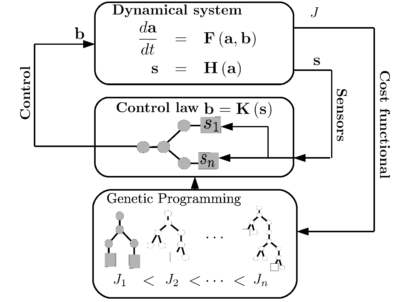
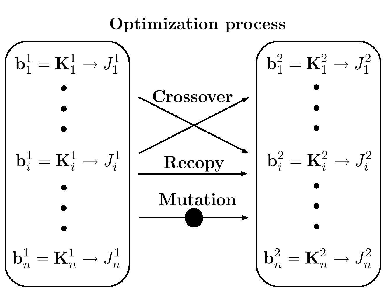
Refer to caption — Figure 1: Left: Control design using MLC. During a learning phase, each control law candidate is evaluated by the dynamical system or experimental plant. This process is iterated over many generations of individuals. At convergence, the best individual (in grey) is determined and used for control. Right: Production of a new generation of individuals. Each individual $K_{i}^{m}$ is ranked by their cost, $J_{i}^{m}$ , $i$ pointing to the $i^{th}$ individual, $m$ to the $m^{th}$ generation. An individual of the subsequent generation can be a copy, a mutation or the result of the cross-over of individuals selected in the preceding generation according to their cost.

The individuals used to produce the new generation are selected based on how well they minimize the cost function. A global extremum of the cost function is typically approximated well in a finite number of generations if the population contains enough diversity to explore the search space. The method has been shown to be successful (Lewis et al., 1992; Nordin & Banzhaf, 1997) even though there is no general mathematical proof for convergence.

3 Control problems

MLC is used to put the system in a desirable state as equilibrium (§3.1), to optimize a given measure on the system such as Lyapunov exponents (§3.2) or the width of a turbulent mixing layer (§3.3).

3.1 Generalized mean-field model

We first consider a generalized mean-field model describing frequency cross-talk for a variety of physical phenomena including fluid flows (Zielinska et al., 1997; Luchtenburg et al., 2009). This model can be viewed as a generalization of the Landau model for the bifurcation from equilibrium to a periodic oscillation. Since we focus on frequency cross-talk, we choose a simple form of this model with two oscillators coupled by a nonlinear variation of one growth rate:

	$\displaystyle\frac{\mathrm{d}}{\mathrm{d}t}\left[\begin{array}[]{c}a_{1}\\ a_{2}\\ a_{3}\\ a_{4}\end{array}\right]=\left[\begin{array}[]{cccc}\sigma_{1}&\omega_{1}&0&0\\ -\omega_{1}&\sigma_{1}&0&0\\ 0&0&\sigma_{2}&\omega_{2}\\ 0&0&-\omega_{2}&\sigma_{2}\end{array}\right]\left[\begin{array}[]{c}{a_{1}}\\ {a_{2}}\\ {a_{3}}\\ {a_{4}}\end{array}\right]+\left[\begin{array}[]{c}0\\ 0\\ 0\\ b\end{array}\right]$
	$\displaystyle\mbox{with }\sigma_{1}=\sigma_{10}-(a_{1}^{2}+a_{2}^{2}+a_{3}^{2}+a_{4}^{2}).$

Hereafter, we denote the sum of squared amplitudes as energy to avoid linguistic sophistication. We set $\omega_{1}=\omega_{2}/10=1$ and $\sigma_{10}=-\sigma_{2}=0.1$ so that the first oscillator $(a_{1},a_{2})$ is unstable at the origin while the other one $(a_{3},a_{4})$ is stable. When uncontrolled ( $b\equiv 0$ ), the nonlinearity drives the first oscillator to nonlinear saturation by the change of total energy. The actuation directly effects only the stable oscillator. This system is arguably the simplest nonlinear dynamical system to exhibit frequency cross-talk. We choose to stabilize the first oscillator around its fixed point $(0,0)$ and thus a cost function which measures the fluctuation energy of that unstable oscillator. For any useful application, the energy used for control is required to be small, hence, we penalize the actuation energy:

J=\left<a_{1}^{2}(t)+a_{2}^{2}(t)+\gamma b^{2}(t)\right>_{T},

(20)

with $\gamma=0.01$ as penalization coefficient and $\left<\cdot\right>_{T}$ denoting the average over the time interval $[0,T]$ . Here, $T=100\times{2\pi}/{\omega_{1}}$ is chosen to allow meaningful statistics. The quadratic form of the state and the actuation in the cost function is a standard choice in control theory. We apply MLC with full-state observation ( $\mathbf{s}\equiv\mathbf{a}$ ) to exploit all potential nonlinear mechanisms to control the unstable oscillator.

Knowing the nonlinearity at stake, an open-loop strategy can be designed: exciting the stable oscillator at frequency $\omega_{2}$ will provoke an energy growth which stabilizes the first oscillator as soon as $a_{1}^{2}+a_{2}^{2}+a_{3}^{2}+a_{4}^{2}>\sigma_{10}$ . Note that the linearization of (3.1) yields two uncoupled oscillators. Thus, the first oscillator is uncontrollable in a linear framework.

3.2 Lorenz system

As second example, we consider the Lorenz system controlled in the third component:

$\displaystyle\frac{\mathrm{d}a_{1}}{\mathrm{d}t}$	$\displaystyle=$	$\displaystyle\sigma\left(a_{2}-a_{1}\right),$
$\displaystyle\frac{\mathrm{d}a_{2}}{\mathrm{d}t}$	$\displaystyle=$	$\displaystyle a_{1}\left(\rho-a_{3}\right)-a_{2},$	(21)
$\displaystyle\frac{\mathrm{d}a_{3}}{\mathrm{d}t}$	$\displaystyle=$	$\displaystyle a_{1}a_{2}-\beta a_{3}+b,$

with full-state feedback $b=K(a_{1},a_{2},a_{3})$ , i.e. $\mathbf{s}\equiv\mathbf{a}$ . The Lorenz system can be stable, periodic or chaotic depending on the set of used parameters. We employ $\sigma=10$ , $\beta=8/3$ and $\rho=20$ , such that the uncontrolled system ( $b\equiv 0$ ) is periodic. Instead of stabilizing an equilibrium, we demonstrate how to obtain a chaotic system. Existing strategies may stabilize or destabilize periodic orbits (Ott et al., 1990; Pyragas, 1992; Schöll & Schuster, 2007). Like de la Fraga & Tlelo-Cuautle (2014), we aim at maximizing the largest Lyapunov exponent $\lambda_{1}$ while penalizing the actuation power with a factor $\gamma$ . If $\lambda_{1}$ is positive, the system is chaotic and well-mixing. We define the cost function, which should be minimized, as:

\begin{array}[]{l l l l}J&=&\exp(-\lambda_{1})+\gamma\left<b^{2}(t)\right>_{T}&\quad\mbox{if}\,\,\sum_{i=1}^{3}\lambda_{i}<0,\\ J&\rightarrow&\infty&\quad\mbox{if}\,\,\sum_{i=1}^{3}\lambda_{i}\geq 0,\end{array}

(22)

where $T=100$ is the integration time and $\lambda_{1}\geq\lambda_{2}\geq\lambda_{3}$ are the Lyapunov exponents. These exponents are obtained by a standard algorithm (Wolf et al., 1985). $J$ is assigned the largest computable real number on the computer if the sum of the Lyapunov exponents is positive or the states exceed the bounds we specify.

3.3 Experimental mixing layer

The TUCOROM mixing layer experimental demonstrator is a dual stream wind tunnel with independently controlled turbines. The test section after the trailing edge of the separating plate is of dimension $width\times height\times length=1.0\times 1.0\times 3.0\,m^{3}$ . In this experiment, the Reynolds number is $Re_{\theta}=U_{c}\theta/\nu=500$ based on convective velocity $U_{c}=(U_{1}+U_{2})/2$ and shear layer momentum thickness $\theta$ . The sensors are made of a rake of 24 hot-wires to record velocity fluctuations on a vertical profile across the shear layer. The actuators are 96 micro jets located at the tip of the separating plate and which can be triggered up to $500\,Hz$ (see figure 2). The machine learning control strategy is applied to maximize the width of the mixing layer,

J=\frac{1}{W},\,\,\mbox{with}\,\,W=\frac{\left<\left[\sum_{i=1}^{24}{s}_{i}^{2}(t)\right]\right>_{T}}{\mbox{max}_{i\in[1,24]}(\left<{s}_{i}^{2}\right>_{T})},

(23)

where ${s}_{i}(t)$ is the velocity fluctuation as recorded by the hot-wire anemometer $i$ , $\left<\cdot\right>_{T}$ is an average of all acquisitions during the evaluation time $T=10\,s$ corresponding to about 1000 Kelvin-Helmholtz period. This cost function is minimized when the width $W$ of the fluctuation energy profile is maximized.

4 Results

In this section, we present the results of the MLC algorithm for the three examples discussed in §3: a system with frequency cross-talk (§4.1), an optimization of chaos (§4.2) and an experiment with a turbulent mixing layer (§4.3).

4.1 Generalized mean-field model

The function space is explored by using a set of elementary ( $+,-,\times,/$ ) and transcendental (e.g. $\exp,\sin,\ln$ ) functions. The functions are ’protected’ to allow them to take arbitrary arguments in $\mathbb{R}$ . Additionally, the actuation command is limited to the range $[-1\,,\,1]$ to emulate an experimental actuator. Up to $50$ generations comprising $1000$ individuals are processed.

The control law ultimately returned by the MLC process corresponds to the best individual of the last generation. The formula is given in §7. It can be summarized as follows:

b=K_{1}(a_{4})\times K_{2}(a_{1},a_{2},a_{3},a_{4}).

(24)

The function $K_{1}(a_{4})$ describes a phasor control that destabilizes the stable oscillator. The function $K_{2}(a_{1},a_{2},a_{3},a_{4})$ acts as a gain dominated by the energy of the unstable oscillator. The performance and the behaviour of the control law are displayed in figure 3. The control law is energizing the second oscillator up to $10^{0}\gg\sigma_{10}$ as soon as the first oscillator has an energy which is larger than $10^{-10}$ . This is stabilizing the unstable oscillator very quickly with a decay scaling roughly as $\exp(-10^{5}t)$ . After stabilization, the control stays at very low values. That keeps the stable oscillator at a correspondingly low energy $\approx 10^{-10}$ , while the amplitude of the unstable oscillator is exponentially increasing with its initial growth rate $\sigma_{10}$ . This control law exploits the frequency cross-talk and vanishes when not needed, i.e. $a_{1}\approx a_{2}\approx 0$ . That control could not be derived from a linearized model of the system. Less energy is used as compared to the best periodic excitation.

4.2 Lorenz system

MLC is applied to the periodic Lorenz system to maximize the largest Lyapunov exponent while keeping the solution bounded. The basic operations that compose the control law are ( $+$ , $-$ , $\times$ , $/$ ) as well as randomly generated constants. The maximum number of generations is chosen as 50 with 1000 individuals each. We consider for $\gamma$ the values of $\gamma_{S}=1$ , $\gamma_{W}=0.01$ and $\gamma_{N}=0$ , representing strong, weak and no penalization of the actuation. This illustrates how the cost function definition influences the problem to be solved. After 50 generations, the best individuals (see §7) associated with strong, weak and no penalization have maximum Lyapunov exponents of $\lambda_{1}=0.715$ , $2.072$ and $17.613$ , respectively. The changes in the system and the control function are displayed in figure 4. The control laws associated with $\gamma_{S}$ and $\gamma_{W}$ are affine expressions of $a_{3}$ and the reduction of the actuation cost leads to a larger amplitude of the feedback. In those cases, the most efficient controls lead the system into behaviours close to the canonical Lorenz system ( $\rho=28$ , $\lambda_{1}=0.905$ ). For $\gamma_{W}$ the nature (from saddle point to spiral saddle point) and the position of the central fixed point from the actuated system are changed. If the actuation is not penalized ( $\gamma=0$ ) the feedback law is a complex nonlinear function of all states. The nature and position of all fixed points are changed as $\lambda_{1}$ reaches higher values.

4.3 Experimental mixing layer

MLC is applied to the TUCOROM experimental mixing layer demonstrator (Parezanović et al., 2013). The selected functions are $(+,-,\times,/,\sin,\cos,\log,\tanh)$ . The micro-jets are turned on if the action command is positive and off otherwise. The number of generations is chosen to be 25 with 100 individuals each. The evaluation of one generation is achieved in 40 minutes of experiment. The employed cost function (23) maximizes the width of the fluctuation energy profile in the shear layer. The control law ultimately returned by the MLC algorithm is compared to the reference open-loop control, an harmonic forcing at the most efficient frequency as determined by a parametric study (see figure 5). While the best open-loop forcing is able to upgrade the cost function value by 55% (compared to the uncontrolled flow), MLC is able to improve it by 67%. Moreover, the total flow-rate through the actuation jets achieved by the MLC closed-loop control is reduced by 46%. These results shall be further detailed in an upcoming publication.

5 Conclusions and future directions

We propose a model-free optimization of sensor-based control laws for general multiple-input multiple-output (MIMO) plants, the ’machine learning control’ (MLC). This strategy is based on genetic programming (GP). GP is one of the most versatile methods for function optimization in machine learning and includes genetic algorithms (GA). While GA performs a parameter identification of a given control law, GP performs also a structure identification of arbitrary nonlinear control laws. Thus, MLC comprises an increasingly popular control optimization based on GA. MLC is based on an ensemble (called ’generation’) of general nonlinear functions (called ’individuals’) and invests in an exploration of novel laws. Thus, MLC has a large chance to detect and exploit otherwise invisible local extrema. In contrast, model-free adaptive control is particularly suited for adjusting one or few parameters of prescribed open- or closed-loop control laws to changing flow conditions. Such online parameter adaptation is not part of the presented MLC method but could — in principle — be included.

As our first test-case, MLC has been successfully applied to a closed-loop stabilization of a generalized two-frequency mean-field model detecting and exploiting frequency cross-talk in an unsupervised manner. Frequency cross-talk is of primordial importance for large-scale turbulence control with complex interactions between the coherent structures at different dominant frequencies, the mean flow changing on large time scales and the cascade to small-scale structures with small associated time scales. By definition, frequency cross-talk is ignored in any linearized system. Another successful demonstration of MLC is closed-loop control for the maximization of the Lyapunov exponent (stretching) of the forced Lorenz equations. Again, this increase of unpredictability is a highly nonlinear phenomenon.

A challenging experimental closed-loop control demonstration is the increase of the mixing layer width in the TUCOROM wind-tunnel (Parezanović et al., 2013). MLC outperforms the best periodic forcing by an additional 12% increase of the mixing layer width and leads to a significant reduction of the actuation cost. It may be noted that this open-loop reference level is also obtained with an extremum seeking method. Expectantly, corresponding adaptive control does not lead to a better mixing. MLC has overcome important technical challenges for in-time control: (1) the hot-wire sensors show broadband frequency dynamics, (2) the large convective time delay from actuators to sensors and (3) this response was found to be strongly nonlinear.

Summarizing, the model-free formulation of MLC gives rise to a high flexibility: it can be applied to any MIMO plant and use any cost function. Though a model is not needed, the more we know about the system, the better we can design the cost function according to the underlying physics and the better we can bias the control law selection. Further improvements can be expected from including actuation or sensor histories, like in ARMAX models (Hervé et al., 2012). The relation of tree depth, number of generations, number of individuals with convergence is subject of ongoing research and may boost the performance considerably.

The major drawback of the model-free approach lies in the evaluation time, as each individual needs a simulation or experiment to be run. This translates in a large time requirement should the process be serial. Consequently, massive parallelization of computations or experiments may be needed in real-world MLC applications. For instance, transition control in a pipe flow may be performed with a grid of 10 times 10 simultaneously used parallel pipes.

The model-free control design is particularly interesting for experimental applications for which a model might not even be known, like for the control of some multi-phase or multi-physics flows with several phases, combustion or unknown non-Newtonian fluids. We conjecture that MLC will play a similar role as control theory in the closed-loop control of turbulence and other complex flows.

6 Acknowledgements

We acknowledge funding of the French Science Foundation ANR (Chaire d’Excellence TUCOROM, SepaCoDe). MS and MA acknowledge the support of the LINC project (no. 289447) funded by EC’s Marie-Curie ITN program (FP7-PEOPLE-2011-ITN). We thank Steven Brunton, Eurika Kaiser and Nathan Kutz for fruitful discussions and comments.

7 Supplementary material

A document displaying the control laws derived by MLC is available as supplementary material. A movie displaying the behaviour of the controlled generalized mean-field model is available as Movie 1. A movie displaying the behaviour of the controlled Lorenz system is available as Movie 2

References

Bagheri et al. (2009) Bagheri, S., Brandt, L. & Henningson, D. S. 2009 Input–output analysis, model reduction and control of the flat-plate boundary layer. J. Fluid Mech. 620, 263–298.
Choi et al. (1994) Choi, H., Moin, P. & Kim, J. 1994 Active turbulence control for drag reduction in wall-bounded flows. J. Fluid Mech. 262, 75–110.
Fleming & Purshouse (2002) Fleming, P. J. & Purshouse, R. C. 2002 Evolutionary algorithms in control systems engineering: a survey. Control Engineering Practice 10 (11), 1223–1241.
de la Fraga & Tlelo-Cuautle (2014) de la Fraga, L. G. & Tlelo-Cuautle, E. 2014 Optimizing the maximum Lyapunov exponent and phase space portraits in multi-scroll chaotic oscillators. Nonlinear Dynamics pp. 1–13.
Glezer et al. (2005) Glezer, A., Amitay, M. & Honohan, A. M. 2005 Aspects of low-and high-frequency actuation for aerodynamic flow control. AIAA journal 43 (7), 1501–1511.
Hervé et al. (2012) Hervé, A., Sipp, D., Schmid, P. J. & Samuelides, M. 2012 A physics-based approach to flow control using system identification. J. Fluid Mech. 702, 26–58.
Högberg et al. (2003) Högberg, M., Bewley, T. R. & Henningson, D. S. 2003 Linear feedback control and estimation of transition in plane channel flow. J. Fluid Mech. 481, 149–175.
Illingworth et al. (2012) Illingworth, S. J., Morgans, A. S. & Rowley, C. W. 2012 Feedback control of cavity flow oscillations using simple linear models. J. Fluid Mech. 709, 223–248.
King (2010) King, R. 2010 Active Flow Control II: Papers Contributed to the Conference “Active Flow Control II 2010”, Berlin, Germany, May 26 to 28, 2010, , vol. 108. Springer.
King et al. (2006) King, R., Becker, R., Feuerbach, G., Henning, L., Petz, R., Nitsche, W., Lemke, O. & Neise, W. 2006 Adaptive flow control using slope seeking. In 14th IEEE Mediterranean Conference on Control and Automation, 2006, pp. 1–6.
Koza (1992) Koza, J. R. 1992 Genetic Programming: On the Programming of Computers by Means of Natural Selection. The MIT Press.
Lewis et al. (1992) Lewis, M. A., Fagg, A. H. & Solidum, A. 1992 Genetic programming approach to the construction of a neural network for control of a walking robot. In IEEE International Conference on Robotics and Automation, , vol. 3, pp. 2618–2623.
Luchtenburg et al. (2009) Luchtenburg, D. M., Günter, B., Noack, B. R., King, R. & Tadmor, G. 2009 A generalized mean-field model of the natural and actuated flows around a high-lift configuration. J. Fluid Mech. 623, 283–316.
Luke et al. (2013) Luke, S., Panait, L., Balan, G., Paus, S., Skolicki, Z., Kicinger, R., Popovici, E., Sullivan, K., Harrison, J., Bassett, J., Hubley, R., Desai, A., Chircop, A., Compton, J., Haddon, W., Donnelly, S., Jamil, B., Zelibor, J., Kangas, E., Abidi, F., Mooers, H., O’Beirne, J., Talukder, K. A. & McDermott, J. 2013 A Java-based Evolutionary Computation Research System, http://cs.gmu.edu/ eclab/projects/ecj/.
Nordin & Banzhaf (1997) Nordin, P. & Banzhaf, W. 1997 An on-line method to evolve behavior and to control a miniature robot in real time with genetic programming. Adaptive Behavior 5 (2), 107–140.
Noriega & Wang (1998) Noriega, J. R. & Wang, H. 1998 A direct adaptive neural-network control for unknown nonlinear systems and its application. IEEE Trans. Neural Networks 9 (1), 27–34.
Ott et al. (1990) Ott, E., Grebogi, C. & Yorke, J. A. 1990 Controlling chaos. Phys. Rev. Lett. 64 (11), 1196.
Parezanović et al. (2013) Parezanović, V., Laurentie, J. C., Fourment, C., Cordier, L., Noack, B. R. & Shaqarin, T. 2013 Modification of global properties of a mixing layer by open/closed loop actuation. In Proceedings of the 8th International Symposium On Turbulent and Shear Flow Phenomena.
Pastoor et al. (2008) Pastoor, M., Henning, L., Noack, B. R., King, R. & Tadmor, G. 2008 Feedback shear layer control for bluff body drag reduction. J. Fluid Mech. 608, 161–196.
Pyragas (1992) Pyragas, K. 1992 Continuous control of chaos by self-controlling feedback. Phys. Lett. A 170 (6), 421–428.
Roussopoulos (1993) Roussopoulos, K. 1993 Feedback control of vortex shedding at low Reynolds numbers. J. Fluid Mech. 248, 267–296.
Rowley & Williams (2006) Rowley, C. W. & Williams, D. R. 2006 Dynamics and control of high-Reynolds-number flow over open cavities. Annu. Rev. Fluid Mech. 38 (1), 251–276.
Samimy et al. (2007) Samimy, M., Debiasi, M., Caraballo, E., Serrani, A., Yuan, X., Little, J. & Myatt, J. H. 2007 Feedback control of subsonic cavity flows using reduced-order models. J. Fluid Mech. 579, 315–346.
Schöll & Schuster (2007) Schöll, E. & Schuster, H. G. 2007 Handbook of Chaos Control. Wiley-VCH, Weinheim.
Sipp & Lebedev (2007) Sipp, D. & Lebedev, A. 2007 Global stability of base and mean flows: a general approach and its applications to cylinder and open cavity flows. J. Fluid Mech. 593 (1), 333–358.
Thiria et al. (2006) Thiria, B., Goujon-Durand, S. & Wesfreid, J.E. 2006 The wake of a cylinder performing rotary oscillations. J. Fluid Mech. 560, 123–147.
Wahde (2008) Wahde, M. 2008 Biologically Inspired Optimization Methods: An Introduction. WIT Press.
Wolf et al. (1985) Wolf, A., Swift, J. B., Swinney, H. L. & Vastano, J. A. 1985 Determining Lyapunov exponents from a time series. Physica 16D (3), 285–317.
Zielinska et al. (1997) Zielinska, B. J. A., Goujon-Durand, S., Dǔsek, J. & Wesfreid, J. E. 1997 Strongly nonlinear effect in unstable wakes. Phys. Rev. Lett. 79 (20), 3893.