Stable Graphical Models

Navodit Misra misra@molgen.mpg.de Affiliation: Max Planck Institute for Molecular Genetics Affiliation: Ihnestr. 63-73, 14195 Berlin, Germany Ercan E. Kuruoglu ercan.kuruoglu@isti.cnr.it Affiliation: ISTI-CNR Affiliation: Via G. Moruzzi 1, 56124 Pisa, Italy Affiliation: and Affiliation: Max Planck Institute for Molecular Genetics Affiliation: Ihnestr. 63-73, 14195 Berlin, Germany

Abstract

Stable random variables are motivated by the central limit theorem for densities with (potentially) unbounded variance and can be thought of as natural generalizations of the Gaussian distribution to skewed and heavy-tailed phenomenon. In this paper, we introduce $\alpha$ -stable graphical ( $\alpha$ -SG) models, a class of multivariate stable densities that can also be represented as Bayesian networks whose edges encode linear dependencies between random variables. One major hurdle to the extensive use of stable distributions is the lack of a closed-form analytical expression for their densities. This makes penalized maximum-likelihood based learning computationally demanding. We establish theoretically that the Bayesian information criterion (BIC) can asymptotically be reduced to the computationally more tractable minimum dispersion criterion (MDC) and develop StabLe, a structure learning algorithm based on MDC. We use simulated datasets for five benchmark network topologies to empirically demonstrate how StabLe improves upon ordinary least squares (OLS) regression. We also apply StabLe to microarray gene expression data for lymphoblastoid cells from 727 individuals belonging to eight global population groups. We establish that StabLe improves test set performance relative to OLS via ten-fold cross-validation. Finally, we develop SGEX, a method for quantifying differential expression of genes between different population groups.

^†^†shortheadings: Stable Graphical Models / Misra and Kuruoglu^†^†firstpage: 1

keywords

Bayesian networks, stable distributions, linear regression, structure learning, gene expression, differential expression

1 Introduction

Stable distributions have found applications in modeling several real-life phenomena (Berger and Mandelbrot, 1963; Mandelbrot, 1963; Nikias and Shao, 1995; Gallardo et al., 2000; Achim et al., 2001) and have robust theoretical justification in the form of the generalized central limit theorem (Feller, 1968; Nikias and Shao, 1995; Nolan, 2013). Several special instances of multivariate generalization of stable distributions have also been described in literature (Samorodnitsky and Taqqu, 1994; Nolan and Rajput, 1995). Multivariate stable densities have previously been applied to modeling wavelet coefficients with bivariate $\alpha$ -stable distributions (Achim and Kuruoglu, 2005), inferring parameters for linear models of network flows (Bickson and Guestrin, 2011) and stock market fluctuations (Bonato, 2012).

In this paper, we describe $\alpha$ -stable graphical ( $\alpha$ -SG) models, a new class of multivariate stable densities that can be represented as directed acyclic graphs (DAG) with arbitrary network topologies. We prove that these multivariate densities also correspond to linear regression-based Bayesian networks and establish a model selection criterion that is asymptotically equivalent to the Bayesian information criterion (BIC). Using simulated data for five benchmark network topologies, we empirically show how $\alpha$ -SG models improve structure and parameter learning performance for linear regression networks with additive heavy-tailed noise.

One motivation for the present work comes from potential applications to computational biology, especially in genomics, where Bayesian network models of gene expression profiles are a popular tool (Friedman et al., 2000; Ben-Dor et al., 2000; Friedman, 2004). A common approach to network models of gene expression involves learning linear regression-based Gaussian graphical models. However, the distribution of experimental microarray intensities shows a clear skew and may not necessarily be best described by a Gaussian density (Section 3.2). Another aspect of microarray intensities is that they represent the average mRNA concentration in a population of cells. Assuming the number of mRNA transcripts within each cell to be independent and identically distributed, the generalized central limit theorem suggests that the observed shape should asymptotically (for large population size) approach a stable density (Feller, 1968; Nikias and Shao, 1995; Nolan, 2013). Univariate stable distributions have previously been used to model gene expression data (Salas-Gonzalez et al., 2009a; Salas-Gonzalez et al., 2009b) and it is therefore natural to consider multivariate $\alpha$ -stable densities as models for mRNA expression for larger sets of genes. In Section 3.2 we provide empirical evidence to support this reasoning. We further develop $\alpha$ -stable graphical ( $\alpha$ -SG) models for quantifying differential expression of genes from microarray data belonging to phase III of the HapMap project (International HapMap 3 Consortium and others, 2010; Montgomery et al., 2010; Stranger et al., 2012).

The rest of the paper is structured as follows : Section 2.1 describes the basic notation and background concepts for Bayesian networks and stable densities. Section 2.2 introduces $\alpha$ -SG models and establishes that these models are Bayesian networks that also represent multivariate stable distributions with finite spectral measures. Section 2.3 establishes the equivalence of the popular but (in this case) computationally challenging Bayesian information criterion (BIC) for structure learning and the computationally more tractable minimum dispersion criterion (MDC), for all $\alpha$ -SG models that represent symmetric densities. Furthermore, we establish how data samples from any $\alpha$ -SG model can be combined to generate samples from a partner symmetric $\alpha$ -SG model with identical network topology and regression coefficients. Using these theoretical results we design StabLe, an efficient algorithm that combines ordering-based search (OBS) (Teyssier and Koller, 2005) for structure learning with the iteratively re-weighted least squares (IRLS) algorithm (Byrd and Payne, 1979) for learning the regression parameters via least $l_{p}$ norm estimation. Finally, in Section 3 we implement the structure and parameter learning algorithm on simulated and expression microarray data sets.

2 Methods

In this section we develop the theory and algorithms for learning $\alpha$ -SG models from data. First, we discuss some well-established results for Bayesian networks and $\alpha$ -stable densities.

2.1 Background

We begin with an introduction to Bayesian network models (Pearl, 1988) for the joint probability distribution of a finite set of random variables $\mathcal{X}=\{X_{1},\ldots X_{m}\}$ . A Bayesian network $B(G,\Theta)$ is specified by a directed acyclic graph (DAG) $G$ , whose vertices represent random variables in $\mathcal{X}$ and a set of parameters $\Theta=\{\theta_{i}|X_{i}\in\mathcal{X}\}$ , that determine the conditional probability distribution $p(X_{i}|Pa(X_{i}),\theta_{i})$ for each variable $X_{i}\in\mathcal{X}$ given the state of its parents $Pa(X_{i})\subseteq\mathcal{X}\setminus\{X_{i}\}$ in $G$ (Koller and Friedman, 2009). We will overload the symbols $X_{j}$ and $Pa(X_{j})$ to represent both sets of random variables and their instantiations. The directed acyclic graph $G$ implies a factorization of the joint probability density into terms representing each variable $X_{i}$ and its parents $Pa(X_{i})$ (called a family) such that :

P_{B}(\mathcal{X})=\prod_{i=1}^{|\mathcal{X}|}p(X_{i}|Pa(X_{i}),\theta_{i})

(1)

The dependence of $p(X_{i}|Pa(X_{i}),\theta_{i})$ on $\theta_{i}$ is usually specified by an appropriately chosen family of parametrized probability densities for the random variables, such as Gaussian or $\log$ -Normal. In this paper, we will use multivariate stable densities to model the random variables in $\mathcal{X}$ . The primary motivation for modeling continuous random variables using stable distributions comes from the generalization of the central limit theorem to distributions with unbounded variance (Feller, 1968; Nikias and Shao, 1995). In the limit of large $N$ , all sums of $N$ independent, identically distributed random variables approach a stable density. A formal definition for stable random variables can be provided in terms of the characteristic function (Fourier transform of the density function)

Definition 1.

A stable random variable $X\sim~S_{\alpha}(\beta,\gamma,\mu)$ , is defined for each $\alpha\in(0,2]$ , $\beta\in[-1,1]$ , $\gamma\in(0,\infty)$ and $\mu\in(-\infty,\infty)$ . The probability density $f(X|\alpha,\beta,\gamma,\mu)$ is implicitly specified by a characteristic function $\phi(q|\alpha,\beta,\gamma,\mu)$ :

$\displaystyle\phi(q\|\alpha,\beta,\gamma,\mu)$	$\displaystyle\equiv$	$\displaystyle\mathbb{E}[\exp(\imath qX)]$
	$\displaystyle=$	$\displaystyle\int_{-\infty}^{\infty}f(X\|\alpha,\beta,\gamma,\mu)\exp(\imath qX)dX$
	$\displaystyle=$	$\displaystyle\exp\bigl(\imath\mu q-\gamma\|q\|^{\alpha}[1-\imath\beta~\mathrm{sign}(q)r(q,\alpha)]\bigr)$
$\displaystyle\mathrm{where,}~r(q,\alpha)$	$\displaystyle=$	$\displaystyle\left\{\begin{array}[]{cc}\tan\frac{\alpha\pi}{2}&~\alpha\neq 1\\ -\frac{2}{\pi}\log\|q\|&~\alpha=1\end{array}\right.$

The parameters $\alpha,\beta,\gamma$ and $\mu$ will be called the characteristic exponent, skew, dispersion and location respectively. Unfortunately, the density $f(X|\alpha,\beta,\gamma,\mu)$ does not have a closed-form analytical expression except for the three well-known stable distributions (Figure 1 and Table 1).

Except for the Gaussian case, the asymptotic (large $x$ ) behavior of univariate $\alpha$ -stable densities shows Pareto or power law tails (Lévy, 1925). The following lemma formalizes this observation (Samorodnitsky and Taqqu, 1994; Nolan, 2013)

Lemma 1.

If $X\sim S_{\alpha}(\beta,\gamma,0)$ with $0<\alpha<2$ , then as $x\rightarrow\infty$

	$\displaystyle Pr(X>x)$	$\displaystyle\sim$	$\displaystyle(1+\beta)\gamma C_{\alpha}x^{-\alpha}$
	$\displaystyle C_{\alpha}=(2\int{{}_{0}}{{}^{\infty}}x^{-\alpha}\sin xdx)^{-1}$	$\displaystyle=$	$\displaystyle\frac{1}{\pi}\Gamma(\alpha)\sin(\frac{\alpha\pi}{2})$

Refer to caption — Figure 1: The three instances of analytically known univariate $\alpha$ -stable densities $S_{\alpha}(\beta,\gamma,\mu)$ . Lévy $(\gamma,\mu)\sim S_{0.5}(1,\gamma,\mu)$ (solid blue curves), Cauchy $(\gamma,\mu)\sim S_{1.0}(0,\gamma,\mu)$ (dashed green curves) and Normal $(\mu,\sigma)\sim S_{2.0}(0,\frac{\sigma^{2}}{2},\mu)$ (dot-dashed red curves).

Distribution	$S_{\alpha}(\beta,\gamma,\mu)$	$f(X\|\alpha,\beta,\gamma,\mu)$	Support
Lévy $(\gamma,\mu)$	$S_{0.5}(1,\gamma,\mu)$	$\frac{\gamma}{\sqrt{2\pi}}\frac{1}{(x-\mu)^{3/2}}\exp\bigl(-\frac{\gamma^{2}}{2(x-\mu)}\bigr)$	$\mu<x<\infty$
Cauchy $(\gamma,\mu)$	$S_{1.0}(0,\gamma,\mu)$	$\frac{1}{\pi}\frac{\gamma}{\gamma^{2}+(x-\mu)^{2}}$	$-\infty<x<\infty$
Normal $(\mu,\sigma)$	$S_{2.0}(0,\gamma=\frac{\sigma^{2}}{2},\mu)$	$\frac{1}{2\sqrt{\pi\gamma}}\exp\bigl(-\frac{(x-\mu)^{2}}{4\gamma}\bigr)$	$-\infty<x<\infty$

Table 1: Closed-form analytical expressions for Lévy, Cauchy and Normal densities and the corresponding

\alpha

-stable parameters.

A word on the notation used throughout this paper. We will use the symbol $\|Y\|_{p}=(\sum_{\lambda}|Y_{\lambda}|^{p})^{1/p}$ to represent the $l_{p}$ norm of a vector. The $l_{p}$ norm of a vector representing $N$ instantiations of a random variable $Z$ is related to the $p^{th}$ moment $E(|Z|^{p})=\|Z\|_{p}^{p}/N$ . For heavy-tailed $\alpha$ -stable densities, one convenient method for parameter estimation is via fractional lower order moments (FLOM) for $p<\alpha$ (Hardin Jr, 1984; Nikias and Shao, 1995). Later, we will discuss FLOM-based parameter learning in greater detail (Section 2.4.1).

2.2 $\alpha$ -Stable Graphical Models

We can now introduce Bayesian network models reconstructed from stable densities that have compact representations for the characteristic function. Univariate $\alpha$ -stable densities can be generalized to represent multivariate stable distributions that are defined as follows (Samorodnitsky and Taqqu, 1994),

Definition 2.

A $d$ -dimensional multivariate stable distribution over $\mathcal{X}=\{X_{1},\ldots X_{d}\}$ is defined by an $\alpha\in(0,2]$ , $\mu\in\mathbb{R}^{d}$ and a spectral measure $\Lambda$ over the $d$ -dimensional unit sphere $S_{d}$ , such that the characteristic function

$\displaystyle\Phi(q\|\alpha,\mu,\Lambda)$	$\displaystyle\equiv$	$\displaystyle\mathbb{E}[\exp(\imath q^{T}\mathcal{X})]$
	$\displaystyle=$	$\displaystyle\exp\Big(-\int_{S_{d}}\psi(s^{T}q\|\alpha)\Lambda(ds)+\imath\mu^{T}q\Big)$
$\displaystyle\mathrm{where,}~\psi(u\|\alpha)$	$\displaystyle=$	$\displaystyle\|u\|^{\alpha}(1-\imath~\mathrm{sign}(u)r(u,\alpha))$

Definition 3.

An $\alpha$ -stable graphical ( $\alpha$ -SG) model $B(G,\Theta)$ is a probability distribution over $\mathcal{X}$ such that

		$\displaystyle 1.$	$\displaystyle Z_{j}\equiv X_{j}-\sum_{X_{k}\in Pa(X_{j})}w_{jk}X_{k}\sim S_{\alpha}(\beta_{j},\gamma_{j},\mu_{j})$
		$\displaystyle 2.$	$\displaystyle Z_{j}~\mathrm{is~independent~of}~Z_{k}~,~\mathrm{if}~Z_{j}\neq Z_{k},~\forall X_{j}\in\mathcal{X}$

where $Pa(X_{j})\subseteq\mathcal{X}\setminus\{X_{j}\}$ are the parent nodes of $X_{j}$ in the directed acyclic graph $G$ and $\Theta$ describes the distribution parameters

	$\displaystyle w_{jk}\in\mathbb{R},$		$\displaystyle W_{j}=\{w_{jk}\|X_{k}\in Pa(X_{j})\},$
	$\displaystyle\theta_{j}=\{\alpha,\beta_{j},\gamma_{j},\mu_{j}\}\cup W_{j},$		$\displaystyle\Theta=\{\theta_{i}\|X_{i}\in\mathcal{X}\}$

It is straightforward to see that $B(G,\Theta)$ is indeed a Bayesian network.

Lemma 2.

$B(G,\Theta)$ in Definition 3 represents a Bayesian network

Proof.

Let $d=|\mathcal{X}|$ . First note that every directed acyclic graph can be used to infer an ordering (not necessarily unique) on the variables in $\mathcal{X}$ such that all parents of each variable have a lower order than the variable itself. Suppose we index each variable with its order in an ordering compatible with the DAG, such that $X_{i}$ has order $i$ . The proof rests on the fact that the transformation matrix from $\{Z_{i}\}$ to $\{X_{i}\}$ for such a graph is lower triangular, with each diagonal entry equal to 1. Since the determinant of a triangular matrix equals the product of its diagonal entries, the Jacobian for the transformation (or the determinant of the transformation matrix), $|\frac{\partial(Z_{1},\ldots Z_{d})}{\partial(X_{1},\ldots X_{d})}|=1$ . Furthermore, since the noise variables $Z_{j}$ ’s are independent of each other

$\displaystyle P_{B}(Z_{1},\ldots Z_{d})$	$\displaystyle=$	$\displaystyle\prod_{j=1}^{d}f(Z_{j}\|\alpha,\beta_{j},\gamma_{j},\mu_{j})$
$\displaystyle\mathrm{also,}~p(X_{j}\|Pa(X_{j}),\theta_{j})$	$\displaystyle=$	$\displaystyle f(Z_{j}\|\alpha,\beta_{j},\gamma_{j},\mu_{j})$
$\displaystyle\implies P_{B}(\mathcal{X})$	$\displaystyle=$	$\displaystyle P_{B}(Z_{1},\ldots Z_{d})\|\frac{\partial(Z_{1},\ldots Z_{d})}{\partial(X_{1},\ldots X_{d})}\|$
$\displaystyle\implies P_{B}(\mathcal{X})$	$\displaystyle=$	$\displaystyle\prod_{j=1}^{d}p(X_{j}\|Pa(X_{j}),\theta_{j})\|\frac{\partial(Z_{1},\ldots Z_{d})}{\partial(X_{1},\ldots X_{d})}\|$
$\displaystyle\implies P_{B}(\mathcal{X})$	$\displaystyle=$	$\displaystyle\prod_{j=1}^{d}p(X_{j}\|Pa(X_{j}),\theta_{j})$

Hence, $B(G,\Theta)$ is a Bayesian network. ∎

Before establishing the fact that an $\alpha$ -SG model is a multivariate stable density in the sense of Definition 2, we prove the following result (proof is provided in Appendix A) :

Lemma 3.

Every $d$ -dimensional distribution with a characteristic function of the form

\Phi(q|\alpha,\tilde{\mu},\Lambda)=\prod_{k=1}^{d}\phi(c_{k}^{T}q|\alpha,\beta_{k},\gamma_{k},\mu_{k})~~\mathrm{where,}~c_{k},q\in\mathbb{R}^{d}

represents a multivariate stable distribution with a finite spectral measure $\Lambda$ .

We are now in a position to establish that $\alpha$ -SG models imply a multivariate stable density with a spectral measure concentrated on a finite number of points over the unit sphere.

Lemma 4.

Every $\alpha$ -SG model represents a multivariate stable distribution with a finite spectral measure of the form in Lemma 3.

Proof.

We will prove the lemma by induction. First, observe that every Bayesian network can be used to assign an ordering (not unique) such that $Pa(X_{j})\subseteq\{X_{1}\ldots X_{j}-1\}$ . As before, we will use such an ordering to index each random variable in $\mathcal{X}$ , such that $X_{|\mathcal{X}|}$ has no descendants. The base case of the lemma, where $|\mathcal{X}|=1$ is clearly true. Assume that the lemma is true for all Bayesian networks with $|\mathcal{X}|=m-1$ . Then for any Bayesian network $B$ with $|\mathcal{X}|=m$ random variables

$\displaystyle\Phi_{B}(q)$	$\displaystyle\equiv$	$\displaystyle\mathbb{E}[\exp(\imath q^{T}\mathcal{X})]$
	$\displaystyle=$	$\displaystyle\int\prod_{j=1}^{\|\mathcal{X}\|}dX_{j}f(Z_{j}\|\alpha,\beta_{j},\gamma_{j},\mu_{j})\exp(\imath q_{j}X_{j})$
	$\displaystyle=$	$\displaystyle\int\Big[\prod_{j=1}^{m-1}dX_{j}f(Z_{j}\|\alpha,\beta_{j},\gamma_{j},\mu_{j})\exp(\imath q_{j}X_{j})\Big]\int dX_{m}f(Z_{m}\|\alpha,\beta_{m},\gamma_{m},\mu_{m})\exp(\imath q_{m}X_{m})$
	$\displaystyle=$	$\displaystyle\int\Big[\prod_{j=1}^{m-1}dX_{j}f(Z_{j}\|\alpha,\beta_{j},\gamma_{j},\mu_{j})\exp(\imath\tilde{q_{j}}X_{j})\Big]\int dZ_{m}f(Z_{m}\|\alpha,\beta_{m},\gamma_{m},\mu_{m})\exp(\imath q_{m}Z_{m})$
	$\displaystyle=$	$\displaystyle\Phi_{\tilde{B}}(\tilde{q})\phi(q_{m}\|\alpha,\beta_{m},\gamma_{m},\mu_{m})$
		$\displaystyle\mathrm{where}~\tilde{B}~\mathrm{is~the~Bayes~net~on}~\tilde{\mathcal{X}}=\mathcal{X}\setminus\{X_{m}\},$
		$\displaystyle\mathrm{and}~\tilde{q}_{j}=q_{j}+w_{mj}q_{m}\|Pa(X_{m})\cap\{X_{j}\}\|~\forall~X_{j}\in\tilde{\mathcal{X}}$

Since by assumption,

$\displaystyle\Phi_{\tilde{B}}(\tilde{q})$	$\displaystyle=$	$\displaystyle\prod_{k=1}^{m-1}\phi(s_{k}^{T}\tilde{q}\|\alpha,\beta_{k},\gamma_{k},\mu_{k})$
$\displaystyle\implies\Phi_{B}(q)$	$\displaystyle=$	$\displaystyle\phi_{\tilde{B}}(\tilde{q})\phi(q_{m}\|\alpha,\beta_{m},\gamma_{m},\mu_{m})$
	$\displaystyle=$	$\displaystyle\prod_{k=1}^{m}\phi(\tilde{s}_{k}^{T}q\|\alpha,\beta_{k},\gamma_{k},\mu_{k}),~\mathrm{where:}$
$\displaystyle\tilde{s}_{k}^{T}q$	$\displaystyle=$	$\displaystyle\left\{\begin{array}[]{cc}\sum_{j=1}^{m-1}s_{k,j}(q_{j}+w_{mj}q_{m}\|Pa(X_{m})\cap\{X_{j}\}\|)&k<m\\ q_{m}&k=m\end{array}\right.$

Therefore, $\Phi_{B}(q)$ represents a $m$ -dimensional multivariate stable distribution with a finite spectral measure (Lemma 3). Therefore, by induction, every $\alpha$ -SG model represents a multivariate stable distribution with a finite spectral measure of the form in Lemma 3. ∎

2.3 Learning $\alpha$ -SG Models

It is straight forward to use the characterization of stable random variables in Definition 1 to verify the following well-known properties (Samorodnitsky and Taqqu, 1994),

Property 1.

If $X_{1}\sim S_{\alpha}(\beta_{1},\gamma_{1},\mu_{1})$ and $X_{2}\sim S_{\alpha}(\beta_{2},\gamma_{2},\mu_{2})$ are independent stable random variables, then $Y=X_{1}+X_{2}\sim S_{\alpha}(\beta,\gamma,\mu)$ , with

\displaystyle\beta=\frac{\beta_{1}\gamma_{1}+\beta_{2}\gamma_{2}}{\gamma_{1}+\gamma_{2}}~,

\displaystyle\gamma=(\gamma_{1}+\gamma_{2})~,

\displaystyle\mu=\mu_{1}+\mu_{2}

Property 2.

If $X\sim S_{\alpha}(\beta,\gamma,\mu)$ and $c,d\in\mathbb{R}$ , then

\displaystyle cX+d

\displaystyle\sim

\displaystyle\left\{\begin{array}[]{cc}S_{\alpha}\Big(\mathrm{sign}(c)\beta,|c|^{\alpha}\gamma,c\mu+d\Big)~,&\alpha\neq 1\\ S_{\alpha}\Big(\mathrm{sign}(c)\beta,|c|\gamma,c(\mu-\frac{2\gamma\beta\ln|c|}{\pi})+d\Big)~,&\alpha=1\end{array}\right.

A popular method for structure learning in Bayesian network models is based on the Bayesian information criterion (BIC) which is also equivalent to the minimum description length (MDL) principle (Schwarz, 1978; Heckerman et al., 2000).

Definition 4.

Given a data set $D=\{D_{1},\ldots,D_{N}\}$ , the Bayesian Information Score $S_{BIC}(B|D)$ for a Bayesian network $B(G,\Theta)$ is defined as,

S_{BIC}(B|D)=\sum_{D_{\lambda}\in D}\log\big[P_{B}(D_{\lambda})\big]-\sum_{X_{i}\in\mathcal{X}}\frac{|Pa(X_{i})|}{2}\log N

The Bayesian information criterion (BIC) selects the Bayesian network that maximizes this score over the space of all directed acyclic graphs $G$ and parameters $\Theta$ .

The major stumbling block in using stable densities is due to the fact that there is no known closed-form analytical expression for them (apart from special cases representing Gaussian, Cauchy and Levy distributions). This makes BIC based inference computationally demanding due to the marginal likelihood term $P_{B}[D_{\lambda}]$ . One main contribution of this paper is an efficient method of learning the network structure and parameters for $\alpha$ -SG models. The next lemma establishes a new result that is useful in efficiently solving the learning problem.

Lemma 5.

Given a data set $D_{Y}=\{Y_{1},\ldots,Y_{N}\}$ generated from a stable random variable $Y\sim S_{\alpha}(\beta,\gamma,\mu)$

$\displaystyle\sum_{\lambda=1}^{N}\log\big[f(Y_{\lambda}\|\alpha,\beta,\gamma,\mu)\big]$	$\displaystyle=$	$\displaystyle-N\Big(\log\gamma+h(Y\|\alpha,\beta)\Big)$
$\displaystyle\mathrm{where,}\lim_{N\rightarrow\infty}h(Y\|\alpha,\beta)$	$\displaystyle=$	$\displaystyle-\int dYf(Y\|\alpha,\beta,1,0)\log f(Y\|\alpha,\beta,1,0)$
	$\displaystyle=$	$\displaystyle H\Big[S_{\alpha}(\beta,1,0)\Big]$

Proof.

Since $Y$ includes samples from a stable distribution, $Y\sim S_{\alpha}(\beta,\gamma,\mu)$ by definition, performing a change of variable to

	$\displaystyle Y\rightarrow\tilde{Y}$	$\displaystyle=$	$\displaystyle\frac{Y}{\gamma^{1/\alpha}}-\tilde{\mu}$		(11)
	$\displaystyle\mathrm{where,}~\tilde{\mu}$	$\displaystyle=$	$\displaystyle\left\{\begin{array}[]{cc}\frac{\mu}{\gamma^{1/\alpha}}&~\alpha\neq 1\\ \frac{\mu}{\gamma}+\frac{2\beta\ln\gamma}{\pi}&~\alpha=1\end{array}\right.$

we get, the standard form density $\tilde{Y}\sim S_{\alpha}(\beta,1,0)$ using Property 2. Furthermore, samples from the transformed data set $\tilde{Y}=\{\tilde{Y}_{1},\ldots,\tilde{Y}_{N}\}$ are also distributed according to the following standard density :

f(Y|\alpha,\beta,\gamma,\mu)=f(\tilde{Y}|\alpha,\beta,1,0)\frac{d\tilde{Y}}{dY}=f(\tilde{Y}|\alpha,\beta,1,0)\frac{1}{\gamma^{1/\alpha}}

This implies that if we know the parameters $\alpha,\beta,\gamma$ and $\mu$ for the density generating $D_{Y}$

$\displaystyle\log\big[f(Y\|\alpha,\beta,\gamma,\mu)\big]$	$\displaystyle=$	$\displaystyle\sum_{\lambda=1}^{N}\log f(Y_{\lambda}\|\alpha,\beta,\gamma,\mu)$
	$\displaystyle=$	$\displaystyle\sum_{j=1}^{N}\Big\{-\frac{\log\gamma}{\alpha}+\log f(\tilde{Y_{j}}\|\alpha,\beta,1,0)\Big\}$
	$\displaystyle=$	$\displaystyle-N\Big(\frac{\log\gamma}{\alpha}+h(Y\|\alpha,\beta)\Big)$

where, $h(Y|\alpha,\beta)$ is defined by

h(Y|\alpha,\beta)\equiv-\frac{1}{N}\sum_{j=1}^{N}\log f(\tilde{Y_{j}}|\alpha,\beta,1,0)

(15)

Here $\tilde{Y}_{j}$ and $Y_{j}$ are related via Equation 11 for all $1\leq j\leq N$ . Note that since the transformed variables $\tilde{Y}_{j}$ are samples from $f(\tilde{Y}|\alpha,\beta,1,0)$ , we have the following asymptotic result for large $N$

$\displaystyle\lim_{N\rightarrow\infty}h(Y,\alpha,\beta)$	$\displaystyle=$	$\displaystyle-\lim_{N\rightarrow\infty}\frac{1}{N}\sum_{j=1}^{N}\log f(\tilde{Y_{j}}\|\alpha,\beta,1,0)$
	$\displaystyle=$	$\displaystyle-\int_{-\infty}^{\infty}f(\tilde{Y}\|\alpha,\beta,1,0)\log f(\tilde{Y}\|\alpha,\beta,1,0)dY$
	$\displaystyle=$	$\displaystyle H\Big[S_{\alpha}(\beta,1,0)\Big]$

where, $H[.]$ is the entropy of the corresponding random variable. ∎

As things stand, the entropy $H[.]$ of stable random variables in the standard form is just as difficult to compute as the original log-likelihood and the previous lemma has just transformed one intractable quantity into another. However, there is an important class of models where we can ignore the entropy term during structure learning. These multivariate distributions have a special property that every linear combination of random variables is distributed as a stable distribution $S_{\alpha}(\beta,.,.)$ with the same $\alpha$ and $\beta$ . One scenario when this is true is when the noise term is symmetric i.e. $\beta_{i}=0~\forall~X_{i}\in\mathcal{X}$ . This special case is important since we later show (Lemma 8) that every $\alpha$ -SG model can be easily transformed into a partner symmetric $\alpha$ -SG model with identical network topology and regression coefficients. For all practical purposes, learning the structure of symmetric $\alpha$ -SG models is effectively the same as learning structure of arbitrary $\alpha$ -SG models.

Lemma 6.

Given a symmetric $\alpha$ -stable graphical model for variables in $\mathcal{X}$ ,

	$\displaystyle Z\equiv w^{T}\mathcal{X}=\sum_{X_{j}\in\mathcal{X}}w_{j}X_{j}$	$\displaystyle\sim$	$\displaystyle S\Big(\alpha,\beta(w)=0,\gamma(w),\mu(w)\Big)~,~\forall w\in\mathbb{R}^{\|\mathcal{X}\|}$
	$\displaystyle\mathrm{if,}~\beta_{i}$	$\displaystyle=$	$\displaystyle 0,~\forall X_{i}\in\mathcal{X}$

Proof.

The dispersion $\gamma(w)$ and skewness $\beta(w)$ for the projection $w^{T}\mathcal{X}$ of any $d$ -dimensional stable random density is given by (Samorodnitsky and Taqqu, 1994)

	$\displaystyle\gamma(w)$	$\displaystyle=$	$\displaystyle\int_{S_{d}}\|w^{T}s\|^{\alpha}\Lambda(ds)$
	$\displaystyle\beta(w)$	$\displaystyle=$	$\displaystyle\gamma(w)^{-1}\int_{S_{d}}\mathrm{sign}(w^{T}s)\|w^{T}s\|^{\alpha}\Lambda(ds)$

Since, $\mathcal{X}$ represents a symmetric $\alpha$ -stable graphical model, Lemma 4 implies

	$\displaystyle\beta(w)$	$\displaystyle=$	$\displaystyle\sum_{k=1}^{d}\frac{\|w^{T}c_{k}\|_{2}^{\alpha}\gamma_{k}}{2\gamma(w)}\int_{S_{d}}\Big\{\delta(s-\frac{c_{k}}{\|c_{k}\|_{2}})+\delta(s+\frac{c_{k}}{\|c_{k}\|_{2}})\Big\}\|w^{T}s\|^{\alpha}\mathrm{sign}(w^{T}s)ds$
		$\displaystyle=$	$\displaystyle 0$

∎

We are now in a position to present the main contribution of this paper : an alternative criterion for model selection that is both computationally efficient and comes with robust theoretical guarantees (Lemma 7). The criterion is called minimum dispersion criterion (MDC) and is a penalized version of a technique previously used in signal processing literature for designing filters for heavy-tailed noise (Stuck, 1978).

Definition 5.

Given a data set $D=\{D_{1},\ldots,D_{N}\}$ , the penalized dispersion score $S_{MDC}(B|D)$ for a Bayesian network $B(G,\Theta)$ is defined as,

S_{MDC}(B|D)=-\sum_{X_{i}\in\mathcal{X}}\Big\{N\frac{\log\gamma_{i}}{\alpha}+\frac{|Pa(X_{i})|}{2}\log N\Big\}

The minimum dispersion criterion (MDC) selects the Bayesian network that maximizes this score over the space of all directed acyclic graphs $G$ and parameters $\Theta$ .

Lemma 7.

Given a data set $D=\{D_{1},\ldots,D_{N}\}$ generated by a symmetric $\alpha$ -stable graphical model, $B^{*}(G^{*},\Theta^{*})$ , the minimum dispersion criterion is asymptotically equivalent to the Bayesian information criterion over the search space of all symmetric $\alpha$ -stable graphical models

Proof.

First consider the contribution to BIC score from each family (ie., each random variable and its parents) separately. Let $Z_{j}=X_{j}-\sum_{X_{k}\in Pa(X_{j})}w_{jk}X_{k}$ be any arbitrary set of regression coefficients for a candidate network $B(G,\Theta)$ . Note that the coefficients $W_{j}=\{w_{jk}|X_{k}\in Pa(X_{j})\}$ need not be the true regression coefficients $W_{j}^{*}$ and $B$ need not be the true network $B^{*}$ . We will use the notation $Z_{i,\lambda}$ for the instantiation of $Z_{i}$ in sample $D_{\lambda}\in D$ . Since $D$ includes samples from a symmetric $\alpha$ -stable graphical model, Lemma 6 implies $Z_{j}\sim S_{\alpha}(\beta=0,\gamma_{j},\mu_{j})$ . Therefore, using Lemma 5

	$\displaystyle Fam(X_{j},Pa(X_{j})\|D)$	$\displaystyle\equiv$	$\displaystyle\sum_{\lambda=1}^{N}\log\Big[f(Z_{j,\lambda}\|\alpha,\beta=0,\gamma_{j},\mu_{j})\Big]-\frac{\|Pa(X_{j})\|}{2}\log N$
		$\displaystyle=$	$\displaystyle-N\Big(\frac{\log\gamma_{j}}{\alpha}+h(\tilde{Z}_{j}\|\alpha,\beta=0)\Big)-\frac{\|Pa(X_{j})\|}{2}\log N$

where, as in Equation 15, $Z_{j}$ and $\tilde{Z}_{j}$ are related by the transformation in Equation 11.

$\displaystyle\implies\frac{S_{BIC}(B\|D)}{N}$	$\displaystyle=$	$\displaystyle\sum_{X_{j}\in\mathcal{X}}\frac{Fam(X_{j},Pa(X_{j})\|D)}{N}$
	$\displaystyle=$	$\displaystyle-\sum_{X_{j}\in\mathcal{X}}\Big(\frac{\log\gamma_{j}}{\alpha}+h(Z_{j}\|\alpha,\beta=0)+\frac{\|Pa(X_{j})\|}{2N}\log N\Big)$
$\displaystyle\implies\lim_{N\rightarrow\infty}\frac{S_{BIC}(B\|D)}{N}$	$\displaystyle=$	$\displaystyle\lim_{N\rightarrow\infty}\frac{S_{MDC}(B\|D)}{N}-\|\mathcal{X}\|H[S_{\alpha}(\beta=0,1,0)\big]$

Since, $|\mathcal{X}|H[S_{\alpha}(\beta=0,1,0)]$ is independent of the candidate network structure and regression parameters $\{W_{j}|X_{j}\in\mathcal{X}\}$ , we get the result that for any pair of networks $B$ and $B^{\prime}$

\displaystyle\implies\lim_{N\rightarrow\infty}\frac{1}{N}\Big(S_{BIC}(B|D)-S_{BIC}(B^{\prime}|D)\Big)

\displaystyle=

\displaystyle\lim_{N\rightarrow\infty}\frac{1}{N}\Big(S_{MDC}(B|D)-S_{MDC}(B^{\prime}|D)\Big)

Therefore, asymptotically, $BIC$ is equivalent to $MDC$ when data is generated by a symmetric $\alpha$ -SG graphical model. ∎

We now show how samples from any stable graphical model can be combined to yield samples from a partner symmetric stable graphical model with identical parameters and network topology. This transformation was earlier used by Kuruoglu (2001) in order to estimate parameters from skewed univariate stable densities. We should point out that the procedure described above has the drawback that symmetrized data set has half the sample size.

Lemma 8.

Every $\alpha$ -SG model can be associated with a symmetric $\alpha$ -SG model with identical skeleton and regression parameters.

Proof.

Given a data set $D=\{D_{1},\ldots D_{N}\}$ representing any $\alpha$ -SG model $B(G,\Theta)$ , consider a resampled data set $\widehat{D}=\{\widehat{D_{1}},\ldots\widehat{D_{N_{S}}}\}$ with variable instantiations

\widehat{X_{i,\lambda}}=X_{i,2\lambda}-X_{i,2\lambda-1}~,~\forall\lambda\in\{1,\ldots N_{S}=\lfloor N/2\rfloor\}

These ’bootstrapped’ data samples $\widehat{D_{\lambda}}=\{\widehat{X_{i,\lambda}}|X_{i}\in\mathcal{X}\}$ represent independent instantiations of random variables $\widehat{\mathcal{X}}\equiv\{\widehat{X_{i}}|X_{i}\in\mathcal{X}\}$ . Similarly, we may use the regression parameters $W$ to define resampled noise variables :

\widehat{Z_{j}}\equiv\widehat{X_{j}}-\sum_{\widehat{X_{k}}\in Pa(X_{j})}w_{jk}\widehat{X_{k}}

We now make two observations :

If $Z_{j}=X_{j}-\sum_{X_{k}\in Pa(X_{j})}w_{jk}X_{k}\sim S_{\alpha}(\beta_{j},\gamma_{j},\mu_{j})$ , then using Property 1

\widehat{Z_{j}}\equiv\widehat{X_{j}}-\sum_{\widehat{X_{k}}\in Pa(X_{j})}w_{jk}\widehat{X_{k}}\sim S_{\alpha}(\beta=0,2\gamma_{j},0)

2.

The transformed noise variables $\widehat{Z_{j}}$ are independent of each other.

But these conditions define an $\alpha$ -SG model (Definition 3). Therefore, by Lemma 2, the resampled data is distributed according to a Bayesian network $\widehat{B}(G,\widehat{\Theta})$ such that

$\displaystyle\widehat{Z_{j}}$	$\displaystyle\equiv$	$\displaystyle\widehat{X_{j}}-\sum_{\widehat{X_{k}}\in Pa(X_{j})}w_{jk}\widehat{X_{k}}$
$\displaystyle P_{\widehat{B}}(\widehat{\mathcal{X}})$	$\displaystyle=$	$\displaystyle\prod_{j=1}^{\|\mathcal{X}\|}f(\widehat{Z_{j}}\|\alpha,0,2\gamma_{j},0)$
$\displaystyle\widehat{\theta_{j}}$	$\displaystyle=$	$\displaystyle\{\alpha,\beta=0,2\gamma_{j},0\}\cup W_{j},~\widehat{\Theta}=\{\widehat{\theta_{j}}\|X_{j}\in\mathcal{X}\}$

∎

2.4 The StabLe Algorithm

In this section we describe StabLe, an algorithm for learning the structure and parameters of $\alpha$ -SG models (Algorithm 1). The first step of StabLe is to center and symmetrize the entire data matrix $D_{I}$ in terms of the variables $\widehat{\mathcal{X}}$ , as described in Lemma 8. This is followed by estimating the global parameter $\alpha$ using the method of $\log$ statistics (Kuruoglu, 2001). Finally, structure learning is performed by a modified version of the ordering-based search (OBS) algorithm (Section 2.4.2). The details of parameter estimation and structure learning algorithms are discussed next.

Algorithm 1 StabLe

Input: Input data matrix

D_{I}

, number of random restarts Nreps

Output:

\alpha

-SG model

B(G,\Theta)

over

\mathcal{X}

D\leftarrow Symmetrized(D_{I})

// Symmetrize the data as per Lemma 8

Estimate

\alpha

from

D

// Use log-statistics, Equation 16

Initialize

B(G,\Theta)=\emptyset

for i =1 to Nreps do

Initialize a random ordering

\sigma

B_{\sigma}(G,\Theta)=OBS(D,\alpha,\sigma)

// Ordering-based search, Algorithm 4

S_{MDC}(B_{\sigma}|D)>S_{MDC}(B|D)

then

B=B_{\sigma}

end if

end for

2.4.1 Parameter Learning

First, we describe the algorithms StabLe uses to estimate the characteristic exponent $\alpha$ from the data matrix $D$ , as well as the parameters $\Gamma=\{\gamma_{j}|X_{j}\in\mathcal{X}\}$ and $W_{j}=\{w_{jk}|X_{k}\in Pa(X_{j})\}$ for any given directed acyclic graph $G$ .

Estimating the global parameter $\alpha$ :

Log statistics can be used to estimate the characteristic exponent $\alpha$ from the centered and symmetrized variables in $\widehat{\mathcal{X}}$ (Kuruoglu, 2001).

Algorithm:

Since every linear combination of variables in $\widehat{\mathcal{X}}$ has the same $\alpha$ , if we define

\widehat{X}=\sum_{i=1}^{|\widehat{\mathcal{X}}|}\widehat{X_{i}}~,\mathrm{~then}

$\displaystyle\alpha$	$\displaystyle=$	$\displaystyle\Big(\frac{L_{2}}{\psi_{1}}-\frac{1}{2}\Big)^{-1/2}$	(16)
$\displaystyle L_{2}$	$\displaystyle\equiv$	$\displaystyle\mathbb{E}\Big[\big(\log\|\widehat{X}\|-\mathbb{E}[\log\|\widehat{X}\|]\big)^{2}\Big]$
$\displaystyle\psi_{1}$	$\displaystyle\equiv$	$\displaystyle\frac{d^{2}}{dy^{2}}\Gamma(y)\bigg\|_{y=1}=\frac{\pi^{2}}{6}$

Estimating the dispersion $\gamma_{j}$ , and regression parameters $W_{j}=\{w_{jk}|X_{k}\in Pa(X_{j})\}$

If $\gamma_{j}(W_{j})$ is the dispersion parameter for the distribution of $Z_{j}=X_{j}-\sum_{X_{k}\in Pa(X_{j})}w_{jk}X_{k}$ , then the minimum dispersion criterion selects regression parameters

W^{*}_{j}=\arg\min\frac{1}{\alpha}\log\gamma_{j}(W_{j})

Minimum dispersion regression coefficients are estimated using a connection between the $l_{p}$ -norm of a stable random variable and the dispersion parameter $\gamma$ (Zolotarev, 1957; Kuruoglu, 2001).

Lemma 9.

If $Z\sim S_{\alpha}(0,\gamma,0)$ , then

E(|Z|^{p})=C(p,\alpha)\gamma^{p/\alpha}~~\forall-1<p<\alpha

where,

C(p,\alpha)=\frac{\Gamma(1-\frac{p}{\alpha})}{\Gamma(1-p)\cos(p\frac{\pi}{2})}

Therefore, to within a constant term $\log C(p,\alpha)$ , minimizing $\frac{1}{\alpha}\log\gamma_{j}$ is identical to minimizing the $l_{p}$ -norm $\|Z_{j}\|_{p}\equiv(\sum_{\lambda=1}^{N}|Z_{j,\lambda}|^{p})^{1/p}$ for $-1<p<\alpha$ .

W^{*}_{j}=\arg\min\log\Bigl(\|Z_{j}\|_{p}\Bigr)\equiv\arg\min\log\Bigl((\sum_{\lambda=1}^{N}|Z_{j,\lambda}|^{p})^{1/p}\Bigr)

Algorithm 2 IRLS // Find the least

l_{p}

norm regression coefficients

Input:

N

dimensional vector for instantiations of the child node

Y

N\times M

matrix

X

of instantiations of the parent set

Pa(Y)

, tolerance

\epsilon

and

p\in(0,2]

Output:

M

dimensional vector of regression co-efficients

W^{*}=\arg\min_{W}\|Y-XW\|_{p}

Initialize

W

with OLS co-efficients

W=(X^{T}X)^{-1}(X^{T}Y)

repeat

Initialize buffer for current regression coefficients

\beta=W

Initialize a diagonal

N\times N

matrix

\Omega

from

\beta

for weighted least squares regression

\Omega_{ij}=\delta_{ij}(Y_{i}-(XW)_{i})^{p-2}~\forall i,j\in\{1,\ldots N\}

Update regression coefficients vector

W=(X^{T}\Omega X)^{-1}(X^{T}\Omega Y)

until

\|\beta-W\|_{2}<\epsilon

// Change in regression coefficients is within tolerance

Algorithm:

Minimization of the $l_{p}$ norm is performed by the iteratively least squares (IRLS) algorithm (Byrd and Payne, 1979). Briefly, the IRLS algorithm repeatedly solves an instance of the weighted least squares problem to achieve successive estimates for the least $l_{p}$ norm coefficients (Algorithm 2). IRLS is attractive since rigorous convergence guarantees can be given (Daubechies et al., 2010) and the method is easy to implement since several software packages are available for the weighted least squares problem. Even though the IRLS objective is no longer convex for $p<1.0$ , Daubechies et al. (2010) show that under certain sparsity conditions, the algorithm can recover the true solution. Simulations described in Section 3.1 tend to support this observation.

For experiments described in this manuscript, StabLe used two values of $p$ for $l_{p}$ -norm estimation. For learning regression coefficients during structure learning, IRLS was implemented with $p=\alpha/1.01$ , since lower values tended to give noisier estimates (possibly due to numerical errors). However, we also found that estimating the term $\log C(p,\alpha)$ is prone to numerical errors for small values of $|\alpha-p|$ . Therefore, we ignore this constant term during structure learning since it is common to all candidate structures. StabLe estimates the dispersion parameters $\gamma_{j}$ after structure learning, by computing the $l_{p}$ -norm for $p=\alpha/10.0$ and applying Lemma 9.

Algorithm 3 K2Search

Input: Symmetrized data matrix

D

, fixed ordering

\sigma

and shape parameter

\alpha

Output:

\alpha

- SG model

B(G,\Theta)

given the ordering

\sigma

Initialize

B(G,\Theta)=\emptyset

for

i=2

|\mathcal{X}|

// Find the optimal parent set

Pa(\sigma_{i})

by greedily // adding edges starting from

Pa(\sigma_{i})=\emptyset

repeat

Initialize

noChange=true

Initialize

best=FS(\sigma_{i},Pa(\sigma_{i})|D,\alpha)

AddPa=\emptyset

// Search for a potential parent

for

X_{j}\in\{\sigma_{1}\ldots\sigma_{i-1}\}\setminus Pa(\sigma_{i})

Estimate regression weights

W_{\sigma_{i}}

for parent set

Pa(\sigma_{i})\cup X_{j}

using IRLS

FS(\sigma_{i},Pa(\sigma_{i})\cup X_{j}|D,\alpha)>best

then

best=FS(\sigma_{i},Pa(\sigma_{i})\cup X_{j}|D,\alpha)

// Update best score and

AddPa=X_{j}

// possible new parent

noChange=false

end if

end for

Pa(\sigma_{i})=Pa(\sigma_{i})\cup AddPa

// Add the new parent

until

noChange

true

// Repeat until local optimum

end for

Algorithm 4 OBS // Find the optimal

\alpha

-SG model using OBS

Input: Symmetrized data matrix

D

, shape parameter

\alpha

, initial ordering

\sigma

Output:

\alpha

-SG model

B(G,\Theta)

over

\mathcal{X}

Initialize SG model

B

=K2Search(

D

\sigma

\alpha

)

for

i=1

|\mathcal{X}|-1

Initialize

T_{i}\sigma=Twiddle(i,\sigma)

// New ordering

T_{i}\sigma

by swapping

{\sigma}_{i}

\sigma_{i+1}

\tilde{B}

= K2Search(

D

T_{i}\sigma

\alpha

) // Compute the optimum

\tilde{B}

given

T_{i}\sigma

DS(i)=S_{MDC}(\tilde{B}|D)-S_{MDC}(B|D)

// Set Delta score for the twiddle

end for

repeat

Initialize

noChange=true

Find

a=\arg\max DS(i)

// Find the best twiddle

T_{a}{\sigma}

\tilde{B}

= K2Search(

D

T_{a}{\sigma}

\alpha

) // Compute the optimum given

T_{a}{\sigma}

S_{MDC}(\tilde{B}|D)>S_{MDC}(B|D)

then

\sigma=T_{a}\sigma,~B=\tilde{B}

// Accept the swap and update

\sigma,B

DS(a-1)

(if

a>1

) // Update delta scores for neighbors

a-1

DS(a+1)

(if

a<|\mathcal{X}|-1

) // and

a+1

, if valid

noChange=false

end if

until

noChange

true

// Repeat until local optimum

2.4.2 Structure Learning

Searching the space of all network structures can be performed through any of the popular hill-climbing algorithms. In this paper we used the ordering-based search (OBS) algorithm (Teyssier and Koller, 2005) to search for a local optimum in the space of all directed acyclic graphs. The algorithm starts with an initial ordering $\sigma$ and then learns a DAG consistent with $\sigma$ ( i.e., all parents of each node must have a lower order). This part of structure learning is performed via a subroutine K2Search (Algorithm 3), which is a modified version of the hill-climbing based K2Search algorithm Cooper and Herskovits (1992). K2Search starts with an empty parent set for each node $X_{i}\in\mathcal{X}$ and greedily adds edges until the MDC based score $FS(X_{i},Pa(X_{i})|D,\alpha)=-\frac{N}{\alpha}\log\gamma_{i}-\frac{|Pa(X_{i})|}{2}\log N$ reaches a local maximum. The main difference from Gaussian graphical models (Heckerman et al., 2000; Schmidt et al., 2007) is that K2Search scores each family based on least $l_{p}$ norm instead of ordinary least squares (OLS). Once K2Search has learned the locally optimum DAG for a given ordering $\sigma$ , OBS explores other ordering by performing elementary operations (or ‘twiddles’) that swap the order of successive variables and recomputes the K2Search scores. This process is continued until a local optimum. StabLe also performs a fixed number of random restarts to explore more of the search space. In all experiments reported here we used 10 random restarts. Pseudo code for the methods is described in Algorithms 4 and 3.

3 Empirical Validation

In this section we describe two sets of numerical experiments to assess the performance of StabLe. The first set is based on synthetic data representing five benchmark network topologies (Section 3.1). These experiments test the accuracy and robustness of MDC based learning on simulated data sets where the ground truth (structure and parameters) is known.

For the second set of experiments, we apply StabLe to a gene expression data set (Section 3.2) from Phase III of the HapMap project (International HapMap 3 Consortium and others, 2010). These samples represent microarray measurements of mRNA expression within lymphoblastoid cells from 727 individuals belonging to eight global population groups (Montgomery et al., 2010; Stranger et al., 2012).

For structure learning, we chose ordinary least squares (OLS) based BIC penalized log-likelihood $S_{OLS}(B|D)$ for comparison.

S_{OLS}(B|D)=-\sum_{X_{i}\in\mathcal{X}}\Bigl\{\log\|Z_{i}-\bar{Z}_{i}\|_{2}+\frac{|Pa(X_{i})|}{2}\log N\Bigr\}

(17)

OLS is commonly used for learning Gaussian graphical models and should be identical to StabLe for $\alpha=2.0$ (for that case $S_{OLS}$ and $S_{MDC}$ are the same up to a network and parameter independent term). This comparison allowed us to asses the effect of heavy-tailed noise ( $\alpha<2.0$ ) on learning performance.

3.1 Synthetic Data

We performed numerical experiments based on simulated data sets for five network topologies from the Bayesian network repository ¹¹ 1 A description for each network is available at http://www.cs.huji.ac.il/labs/compbio/Repository.. These were (number of nodes, edges within brackets) : ALARM (37, 46), BARLEY (48, 84), CHILD (20, 25), INSURANCE (27, 52) and MILDEW (35, 46). Adjacency matrix for each network was downloaded from the supplement to Tsamardinos et al. (2006)²² 2 Supplement can be accessed at http://www.dsl-lab.org/supplements/mmhc_paper/mmhc_index.html.. Each node $X_{i}\in\mathcal{X}$ was assigned an additive $\alpha$ -stable noise variable $Z_{i}$ with same parameters $S_{\alpha}(\beta,\gamma,0)$ and each edge was assigned a regression coefficient that was sampled from $[-\frac{\rho}{2},+\frac{\rho}{2}]$ uniformly at random. The $S_{\alpha}(\beta,\gamma,0)$ noise variable was simulated using the method of Chambers et al. (1976). For each set of experiments, we simulated 100 datasets, each with 2000 samples from an $\alpha$ -SG model with randomly chosen regression weights, but fixed network topology and $\alpha$ -stable noise parameters. The goal was to asses StabLe in terms of its performance at structure learning and estimation of stable noise parameters for a variety of regression coefficients.

We performed five sets of experiments for each network, corresponding to different values of $\alpha$ = 0.8, 1.1, 1.4, 1.7, 2.0. For each set of experiments, we chose $\rho=1.0,~\beta=0.9$ and $\gamma=1.0$ . We chose such a high skew ( $\beta=0.9$ ) in the input data to test our algorithm on its ability to symmetrize and correctly learn (possibly) difficult problem instances. Instead of $\beta$ however, we report a related parameter $\theta=\arctan(\beta\tan\alpha\frac{\pi}{2})$ which can be inferred more robustly in practice since it avoids the singularity near $\alpha=2$ (Kuruoglu, 2001). We used the zeroth order signed moments based method for estimating $\theta$ (Kuruoglu, 2001).

\theta_{i}=\frac{\alpha\pi}{2N}\sum_{\lambda=1}^{N}\mathrm{sign}(X_{i,\lambda}),~\forall~X_{i}\in\mathcal{X}

(18)

We report two set of results for each network : structure learning and parameter estimation. For convenience, we describe the results for the ALARM network first (results for other data sets are provided in Appendix B).

3.1.1 Inferred Structure

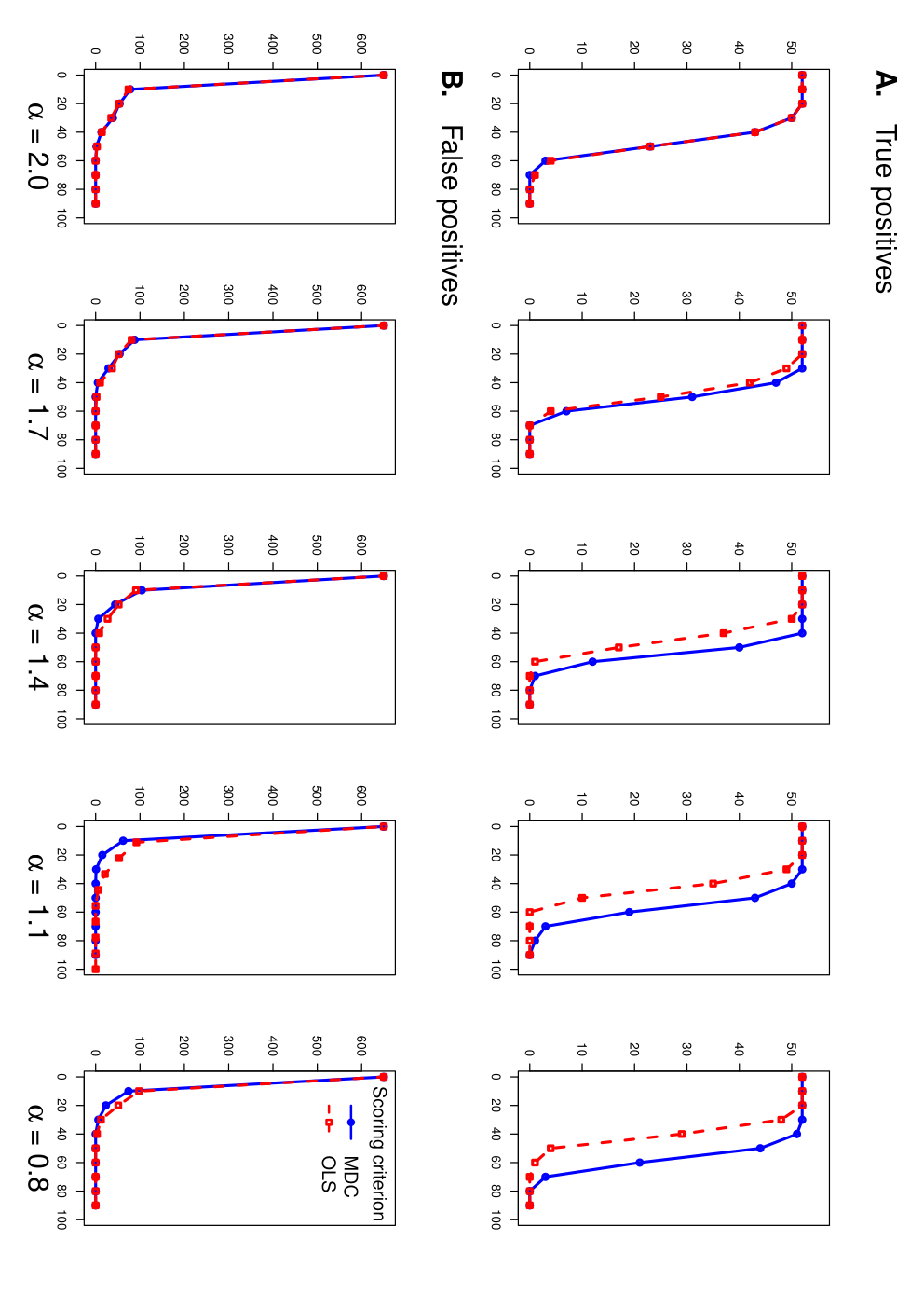
Figure 2 shows the comparative performance of MDC and OLS based approaches. Each curve shows the number of inferred directed edges. Figure 2A, B show the number of true positives and true negatives at a given confidence level (percentage of simulated data sets where the directed edge was learnt). Solid (blue) curves show the performance of MDC and dashed (red) curves show OLS based method. The results are along expected lines with the difference between the two getting larger as $\alpha$ is varied away from 2.0. One clear trend is that while the sensitivity to true positive detection degrades for OLS (Type II errors) as $\alpha$ decreases, the MDC based method remain robust to changes in $\alpha$ . Both methods are however quite reliable at not inferring incorrect edges (false positives or Type I errors). Similar behavior is observed for other data sets as well (Appendix B).

3.1.2 Estimated Parameters

Figure 3 shows the comparative performance of MDC and OLS scores in estimating regression coefficients. Figure 2A shows the bias in mean estimates (in absolute magnitude) and Figure 2B, the standard deviation around the mean in estimated coefficients and are averaged over all true positives and all simulated data sets. Note that each of the 100 simulated data set had regression coefficients sampled independently from $[-1/2,1/2]$ . Both methods perform well in terms of low bias, but OLS had a much higher standard deviation at low $\alpha$ . As with structure learning, this pattern was consistently observed for other network topologies as well (Appendix B).

We also assessed the ability of StabLe to infer $\alpha$ -stable noise parameters accurately and robustly. However, we could not show a comparative performance since OLS scores assume Gaussian noise. Figure 4 shows the box plot and basic statistics for the estimates for $\alpha$ , $\theta$ and $\log\gamma$ from the symmetrized data set (node specific parameters $\theta$ and $\log\gamma$ are reported as averages).

\displaystyle\alpha~,

\displaystyle\theta\equiv\frac{1}{|\mathcal{X}|}\sum_{i}\arctan(\beta_{i}\tan\alpha\frac{\pi}{2})~,

\displaystyle\log\gamma=\frac{1}{|\mathcal{X}|}\sum_{i}\log\gamma_{i}

Both $\alpha$ and $\theta$ estimates have low bias and standard deviation for each of the five data sets. But, $\log\gamma$ estimates show a clear tendency to overestimate the dispersion in noise at very low $\alpha$ . This is however a difficult parameter domain for most existing methods for parameter estimation, even for univariate $\alpha$ stable densities (Kuruoglu, 2001). As with other inferences, the performance of StabLe is again robust to changes in network topology (Appendix B).

3.2 Gene Expression Microarray Data

In this section, we describe two sets of analyses for gene expression microarray data from phase III of the HapMap project³³ 3 Data sets can be downloaded from the Array Express database http://www.ebi.ac.uk/arrayexpress/ using Series Accession Numbers E-MTAB-198 and E-MTAB-264.. Our approach models the set of gene expression profiles as a multivariate stable distribution that can be represented by an $\alpha$ -SG model. The first set of experiments aimed at comparing the prediction accuracy of MDC with OLS-based structure learning via ten-fold cross-validation (Section 3.2.2). The results of these experiments establish the utility of heavy-tailed models for gene expression profiles.

Next, we apply $\alpha$ -SG models to the problem of quantifying differential expression (DE) of a gene between samples belonging to different conditions. This is a common task in gene expression-based analyses in contemporary genomics. However, popular methods for detecting differentially expressed genes usually assume the expression profile for each gene to be independent of others. Based on this assumption, DE quantification is performed by testing the null hypothesis that the $\log$ -expression of each gene is identical across the observed conditions and using the corresponding p-value as a measure of DE. In Section 3.2.3, we develop SGEX, a new technique for quantifying differential expression of each gene that is based on $\alpha$ -SG models. We apply SGEX to quantify the DE for a gene in each population group within the HapMap data. Contrary to most existing methods, SGEX takes into account both the heavy-tailed behavior of gene expression densities, as well as linear dependencies between mRNA expression of different genes.

ID	Ethnicity	Location	# Samples	# Genes/Probes
CEU	Caucasians	Utah, USA	109	21800
CHB	Han Chinese	Beijing, China	80	21800
GIH	Gujarati Indians	Houston, USA	82	21800
JPT	Japanese	Tokyo, Japan	82	21800
LWK	Luhya	Webuye, Kenya	83	21800
MEX	Mexican	Los Angeles, USA	45	21800
MKK	Maasai	Kinyawa, Kenya	138	21800
YRI	Yoruba	Ibadan, Nigeria	108	21800

Table 2: The HapMap III population groups and selected microarray probes as reported by Stranger et al. (2012).

3.2.1 Data Normalization

We downloaded pre-processed data for 727 individuals from eight global population groups as reported in Stranger et al. (2012). Details about the eight population groups are provided in Table 2. For each individual, the input data represented $\log$ -intensities for 21800 microarray probes⁴⁴ 4 Each selected probe mapped to a unique, autosomal Ensembl gene. Ensembl gene IDs are available at http://www.ensembl.org. that were quantile and median normalized, as described in the original paper (Stranger et al., 2012). These microarray intensities provide a measure for mRNA concentration within a sample of lymphoblastoid cells from each individual. Before performing structure learning, we further processed each probe intensity as follows :

1.

The log-intensity $l(i)$ for each probe $i$ was median-centered to obtain transformed log-intensities $ml(i)$ , ie., the number of samples with positive log-intensity was half (or 0.5 less than) the total (=363= $\lfloor 727$ ). This is a standard technique for learning Gaussian graphical models from gene expression data and does not affect the network structure.
2.

The median-centered log-intensities were used to assign a rank $R(i)$ to each probe $i$ , in decreasing order of variance. Even for $\alpha$ -stable distributions, variance of $\log$ transformed data is finite (Kuruoglu, 2001). This is also a standard technique for restricting computing time by selecting a subset of genes with most variation.
3.

The median-centered log-intensities $\{ml(i)|R(i)\leq 21800\}$ were exponentiated to $\mathcal{I}=\{2^{ml(i)}|R(i)\leq 21800\}$ .
4.

The exponentiated-median-centered log-intensities $\mathcal{I}_{k}=\{2^{ml(i)}|R(i)\leq k\leq 21800\}$ for the top $k$ ranked probes were provided as input to StabLe (for cross-validation) and SGEX (for DE quantification, as described in Section 3.2.3). In the experiments reported here $k=100$ .

We estimated $\alpha$ over 1000 resampled bootstrap replicates of the data. This was meant as a diagnostic to assess the heavy-tailed nature of the intensities. As shown in Figure 5A, the data suggests a clear departure from a Gaussian profile.

3.2.2 Cross-validation Analysis

We performed a ten-fold cross-validation for the top 100 ranked probes from the HapMap data. Since we wanted to compare MDC with OLS-based learning, we report goodness of fit of the graphical model $B$ on the test set $T=\{T_{1},\ldots T_{N}\}$ in terms of $\log$ fractional lower order moments :

LFLOM(T|B,p)=\sum_{X_{i}\in\mathcal{X}}\Bigl[\frac{1}{p}\log E(|Z_{i}|^{p})\Bigr]=\sum_{X_{i}\in\mathcal{X}}\Bigl[\frac{1}{p}\log E(|X_{i}-\sum_{X_{j}\in Pa(X_{i})}w_{ij}X_{j}|^{p})\Bigr]

where, $w_{ij}$ represents the regression co-efficient for the edge $(X_{j},X_{i})$ . Clearly, if most of the variation in $X_{i}$ can be explained by the parent set $Pa(X_{i})$ , the corresponding $LFLOM$ will be small. For $p=2$ , $LFLOM$ is identical to the negative log-likelihood for Gaussian graphical models⁵⁵ 5 Note that the noise term $Z_{i}$ has zero mean, since the data is centro-symmetrized before cross-validation.. However, the second order moment diverges for $\alpha<2$ (Lemma 9). Therefore, $LFLOM$ provide a more robust estimate for evaluating the model on test set for heavy-tailed noise ( $\alpha<2$ ).

Figure 5B shows the average (over the ten-folds) of $LFLOM$ for MDC (blue) and OLS-based (red) models. In each case, the curves show the difference in $LFLOM$ between optimal (MDC or OLS) network and an empty network (NULL). This allows us to also assess the deterioration in test set performance by treating each gene as an independent random variable (a common assumption in DE quantification). Although the data set contains only 727 samples, we see a clear improvement in test set performance of $\alpha$ -SG models (MDC curve) relative to Gaussian graphical models (OLS curve).

3.2.3 Quantifying Differential Expression With SGEX

Finally, we discuss SGEX, a new technique for quantifying differential expression using $\alpha$ -SG models. SGEX is based on cross-validation for assessing DE of a gene across different conditions. For the HapMap data, we chose each of the eight population groups in turn as the test set and learnt the optimal $\alpha$ -SG model for the rest of the samples. We then estimated $\Delta LD(i,\eta)$ , the change in negative log-likelihood per sample between the test set set $\eta$ and the training set as a measure of DE for each probe $i$

\Delta LD(i,\eta)=\frac{1}{p}\Bigl[\log E_{\eta}(|Z_{i}|^{p})-\log E_{\bar{\eta}}(|Z_{i}|^{p})\Bigr]~,~p\in(-1,\alpha)

Here, $E_{\eta}(.)$ is the expectation value for population $\eta$ (test set) and $E_{\bar{\eta}}(.)$ for the rest (training set). Note that Lemma 9 guarantees that RHS of the previous equation is indeed independent of $p$ . For the calculation reported here $p=\alpha/1.01$ , just as it was during structure learning. Thus, $\Delta LD(i,\eta)$ measures the average increase (or decrease) in log-dispersion for the noise variable $Z_{i}$ corresponding to probe $i$ within population $\eta$ . This density is represented as a heat map in Figure 5C. We should point out that a higher (or lower) dispersion for the noise variable associated with a gene in the test set does not necessarily imply over (or under) expression of a gene in the test set population. The change in dispersion could also be due to a change in network topology or regression coefficients for the test set population.

4 Discussion

In this paper we have introduced and developed the theory for efficiently learning $\alpha$ -SG models from data. In particular, one of the main contributions of this paper is to show how the BIC can be asymptotically reduced to the MDC for $\alpha$ -SG models. This result makes it feasible to efficiently learn the structure of these models, since the log-likelihood term does not have a closed form expression in general. We have also empirically validated the resultant algorithm StabLe on both simulated and microarray data. In both cases, the presence of heavy-tailed noise has a clear effect on learning performance of OLS based methods. Based on these results, we recommend a bootstrapped estimation of $\alpha$ as an effective and computationally efficient diagnostic to assess the applicability of OLS based Gaussian graphical models.

We have also described SGEX, a new technique for quantifying differential expression from microarray data. $\alpha$ -SG models may also have wider applicability to other aspects of computational biology, especially to data from next-generation sequencing technologies. In addition to mRNA expression measurements (RNA-seq experiments), $\alpha$ -SG models may prove helpful for other experiments, such as protein-DNA binding (ChIP-seq experiments) and DNA accessibility measurements (DNase-seq and FAIRE-seq experiments).

Finally, we should mention that there are several potential applications of $\alpha$ -SG models beyond computational biology. In particular, image processing provides several problem instances where there is a need to relate different regions of the image. For example, functional magnetic resonance imaging (fMRI) experiments generate a series of images highlighting activity sites in the brain in response to stimuli. Bayesian networks are an effective way of modeling statistical relations between different areas of the brain and the stimuli (Li et al., 2011). Stable distributions may provide a better model for such applications. Another image processing application with potentials for $\alpha$ -SG models is remote sensing images of the earth (Mustafa et al., 2012) where image histograms demonstrate clearly skewed and heavy tailed characteristics (Kuruoglu and Zerubia, 2004). Traffic modeling (Castillo et al., 2012) and financial data analysis (Bonato, 2012) are also promising application areas.

5 Software Availability

Source code for StabLe and data sets used here are available at
https://sourceforge.net/projects/sgmodels/.

References

Achim and Kuruoglu (2005) A. Achim and E. E. Kuruoglu. Image denoising using bivariate $\alpha$ -stable distributions in the complex wavelet domain. IEEE Signal Processing Letters, 12(1):17–20, 2005.
Achim et al. (2001) A. Achim, A Bezerianos, and P. Tsakalides. Novel Bayesian multiscale method for speckle removal in medical ultrasound images. IEEE Transactions on Medical Imaging, 20(8):772–783, 2001.
Ben-Dor et al. (2000) A. Ben-Dor, L. Bruhn, N. Friedman, I. Nachman, M. Schummer, and Z. Yakhini. Tissue classification with gene expression profiles. Journal of Computational Biology, 7(3-4):559–583, 2000.
Berger and Mandelbrot (1963) J. Berger and B. Mandelbrot. A new model for error clustering in telephone circuits. IBM Journal of Research and Development, pages 224–236, 1963.
Bickson and Guestrin (2011) D. Bickson and C. Guestrin. Inference with multivariate heavy-tails in linear models. In Proceedings of NIPS, 2011.
Bonato (2012) M. Bonato. Modeling fat tails in stock returns: a multivariate stable-GARCH approach. Computational Statistics, 27(3):499–521, 2012.
Byrd and Payne (1979) R. H. Byrd and D. A. Payne. Convergence of the iteratively reweighted least squares algorithm for robust regression. Technical Report 313, The Johns Hopkins University, Baltimore, MD, 1979.
Castillo et al. (2012) E. Castillo, M. Nogal, M. Menéndez, J., S. Sánchez-Cambronero, and P. Jiménez. Stochastic demand dynamic traffic models using generalized beta-Gaussian Bayesian networks. IEEE Transactions on Intelligent Transportation Systems, 13(2):565–581, 2012.
Chambers et al. (1976) J. Chambers, C. Mallows, and B. Stuck. A method for simulating stable random variables. Journal of the American Statistical Association, 71(354):340–344, 1976.
Cooper and Herskovits (1992) G. Cooper and E. Herskovits. A Bayesian method for the induction of probabilistic networks from data. Machine Learning, 9:309–347, 1992.
Daubechies et al. (2010) I. Daubechies, R. DeVore, M. Fornasier, and C. S. Güntürk. Iteratively reweighted least squares minimization for sparse recovery. Communications on Pure and Applied Mathematics, LXIII:1–38, 2010.
Feller (1968) W. Feller. An Introduction to Probability Theory, vol. I, vol. II. John Wiley, New York, 1968.
Friedman (2004) N. Friedman. Inferring cellular networks using probabilistic graphical models. Science, 303(5659):799–805, 2004.
Friedman et al. (2000) N. Friedman, M. Linial, I. Nachman, and D. Pe’er. Using Bayesian networks to analyze expression data. Journal of computational biology, 7(3-4):601–620, 2000.
Gallardo et al. (2000) J. R. Gallardo, D. Makrakis, and L. Orozco-Barbosa. Use of $\alpha$ -stable self-similar stochastic processes for modeling traffic in broadband networks. Performance Evaluation, 40(1):71–98, 2000.
Hardin Jr (1984) C. D. Hardin Jr. Skewed stable variables and processes. Technical Report 79, Univ. North Carolina, Chapel Hill, 1984.
Heckerman et al. (2000) D. Heckerman, D. Chickering, C. Meek, R. Rounthwaite, and C. Kadie. Dependency networks for density estimation, collaborative filtering, and data visualization. Journal of Machine Learning Research, 1:49–75, 2000.
International HapMap 3 Consortium and others (2010) International HapMap 3 Consortium and others. Integrating common and rare genetic variation in diverse human populations. Nature, 467(7311):52–58, 2010.
Koller and Friedman (2009) D. Koller and N. Friedman. Probabilistic graphical models: principles and techniques. MIT press, Cambridge, MA, 2009.
Kuruoglu (2001) E. E. Kuruoglu. Density parameter estimation of skewed $\alpha$ -stable distributions. IEEE Transactions on Signal Processing, 49(10):2192–2201, 2001.
Kuruoglu and Zerubia (2004) E. E. Kuruoglu and J. Zerubia. Modeling SAR images with a generalization of the Rayleigh distribution. IEEE Transactions on Image Processing, 13(4):527–533, 2004.
Lévy (1925) P. Lévy. Calcul des probabilités. Gauthier-Villars Paris, 1925.
Li et al. (2011) R. Li, K. Chen, A. S. Fleisher, E. M. Reiman, L. Yao, and X. Wu. Large-scale directional connections among multi resting-state neural networks in human brain: A functional mri and bayesian network modeling study. NeuroImage, 56(3):1035–1042, 2011.
Mandelbrot (1963) B. Mandelbrot. The variation of certain speculative prices. Journal of Business, 26:394–419, 1963.
Montgomery et al. (2010) S. B. Montgomery et al. Transcriptome genetics using second generation sequencing in a caucasian population. Nature, 464(7289):773–777, 2010.
Mustafa et al. (2012) Y. T. Mustafa, V. A. Tolpekin, and A. Stein. Application of the expectation maximization algorithm to estimate missing values in gaussian bayesian network modeling for forest growth. IEEE Transactions on Geoscience and Remote Sensing, 50(5):1821–1831, 2012.
Nikias and Shao (1995) C. L. Nikias and M. Shao. Signal Processing with Alpha-Stable Distributions. Wiley, New York, 1995.
Nolan (2013) J. P. Nolan. Stable Distributions - Models for Heavy Tailed Data. Birkhäuser, Boston, Chapter 1 online at academic2.american.edu/ jpnolan edition, 2013.
Nolan and Rajput (1995) J. P. Nolan and B. Rajput. Calculation of multi-dimensional stable densities. Communications in Statistics - Simulation and Computation, 24(3):551–566, 1995.
Pearl (1988) J. Pearl. Probabilistic Reasoning in Intelligent Systems. Morgan Kaufmann, San Mateo, CA, 1988.
Salas-Gonzalez et al. (2009a) D. Salas-Gonzalez, E. E. Kuruoglu, and D. P. Ruiz. Modelling and assessing differential gene expression using the alpha stable distribution. The International Journal of Biostatistics, 5(1):1–24, 2009a.
Salas-Gonzalez et al. (2009b) D. Salas-Gonzalez, E. E. Kuruoglu, and D. P. Ruiz. A heavy-tailed empirical bayes method for replicated microarray data. Computational Statistics & Data Analysis, 53(5):1535–1546, 2009b.
Samorodnitsky and Taqqu (1994) G. Samorodnitsky and M. S. Taqqu. Stable Non-Gaussian Random Processes. Chapman and Hall, New York, 1994.
Schmidt et al. (2007) M. Schmidt, A. Niculescu-Mizil, and K. Murphy. Learning graphical model structure using L1-regularization paths. In Proceedings of AAAI, 2007.
Schwarz (1978) G. Schwarz. Estimating the dimension of a model. Annals of Statistics, 6:461–464, 1978.
Stranger et al. (2012) B. E. Stranger et al. Patterns of cis regulatory variation in diverse human populations. PLoS genetics, 8(4):e1002639, 2012.
Stuck (1978) B. W. Stuck. Minimum error dispersion linear filtering of scalar symmetric stable processes. IEEE Transactions on Automatic Control, 23:507–509, 1978.
Teyssier and Koller (2005) M. Teyssier and D. Koller. Ordering-based search: A simple and effective algorithm for learning Bayesian networks. In Proceedings of Uncertainty in Artificial Intelligence (UAI), 2005.
Tsamardinos et al. (2006) I. Tsamardinos, L. E. Brown, and C. F. Aliferis. The max-min hill-climbing Bayesian network structure learning algorithm. Machine learning, 65(1):31–78, 2006.
Zolotarev (1957) V. M. Zolotarev. Mellin-Stieltjes transforms in probability theory. Theory Probability Appl, 2:433–460, 1957.

Appendix A

In this section we provide the proof for Lemma 3

Lemma 3 Every $d$ -dimensional distribution with a characteristic function of the form

\Phi(q|\alpha,\tilde{\mu},\Lambda)=\prod_{k=1}^{d}\phi(c_{k}^{T}q|\alpha,\beta_{k},\gamma_{k},\mu_{k})~~\mathrm{where,}~c_{k},q\in\mathbb{R}^{d}

represents a multivariate stable distribution with a finite spectral measure $\Lambda$ .

Proof.

Assume the following ansatz for the spectral measure $\Lambda$ ,

	$\displaystyle\Lambda_{k}$	$\displaystyle=$	$\displaystyle\frac{\\|c_{k}\\|_{2}^{\alpha}\gamma_{k}}{2}\Big((1+\beta_{k})\delta(s-\frac{c_{k}}{\\|c_{k}\\|_{2}})+(1-\beta_{k})\delta(s+\frac{c_{k}}{\\|c_{k}\\|_{2}})\Big)$
	$\displaystyle\Lambda(ds)$	$\displaystyle=$	$\displaystyle\sum_{k}\Lambda_{k}ds$

and location vector $\tilde{\mu}$ ,

	$\displaystyle\eta_{k}(c_{k}\|\alpha,\beta_{k},\gamma_{k},\mu_{k})$	$\displaystyle=$	$\displaystyle\left\{\begin{array}[]{cc}\mu_{k}&\alpha\neq 1\\ \mu_{k}-\frac{2\beta_{k}\gamma_{k}}{\pi}\log\\|c_{k}\\|_{2}&\alpha=1\end{array}\right.$
	$\displaystyle\tilde{\mu}$	$\displaystyle=$	$\displaystyle\sum_{k=1}^{d}\eta_{k}(c_{k}\|\alpha,\beta_{k},\gamma_{k},\mu_{k})c_{k}~\in\mathbb{R}^{d}$

Upon substitution into the parametrization in Definition 2 we get

$\displaystyle\int_{S_{d}}\psi(s^{T}q\|\alpha)\Lambda_{k}ds$	$\displaystyle=$	$\displaystyle\frac{\\|c_{k}\\|_{2}^{\alpha}\gamma_{k}}{2}\Big((1+\beta_{k})\psi(\frac{c_{k}^{T}q}{\\|c_{k}\\|_{2}}\|\alpha)+(1-\beta_{k})\psi(-\frac{c_{k}^{T}q}{\\|c_{k}\\|_{2}}\|\alpha)\Big)$
	$\displaystyle=$	$\displaystyle\frac{\\|c_{k}\\|_{2}^{\alpha}\gamma_{k}}{2}\frac{\|c_{k}^{T}q\|^{\alpha}}{\\|c_{k}\\|_{2}^{\alpha}}\Big((1+\beta_{k})(1-\imath\mathrm{sign}(c_{k}^{T}q)r(\frac{c_{k}^{T}q}{\\|c_{k}\\|_{2}},\alpha))$
	$\displaystyle+$	$\displaystyle(1-\beta_{k})(1+\imath\mathrm{sign}(c_{k}^{T}q)r(\frac{c_{k}^{T}q}{\\|c_{k}\\|_{2}},\alpha))\Big)$
$\displaystyle\implies\int_{S_{d}}\psi(s^{T}q\|\alpha)\Lambda_{k}.ds$	$\displaystyle=$	$\displaystyle\gamma_{k}\|c_{k}^{T}q\|^{\alpha}\Big(1-\imath\beta_{k}\mathrm{sign}(c_{k}^{T}q)r(\frac{c_{k}^{T}q}{\\|c_{k}\\|_{2}},\alpha)\Big)$
	$\displaystyle=$	$\displaystyle\gamma_{k}\|c_{k}^{T}q\|^{\alpha}\Big(1-\imath\beta_{k}\mathrm{sign}(c_{k}^{T}q)r(c_{k}^{T}q,\alpha)\Big)$
	$\displaystyle-$	$\displaystyle\imath\beta_{k}\gamma_{k}\|c_{k}^{T}q\|^{\alpha}\mathrm{sign}(c_{k}^{T}q)\Big(r(\frac{c_{k}^{T}q}{\\|c_{k}\\|_{2}},\alpha)-r(c_{k}^{T}q,\alpha)\Big)$

$\displaystyle\mathrm{Since,}~r(\frac{c_{k}^{T}q}{\\|c_{k}\\|_{2}},\alpha)-r(c_{k}^{T}q,\alpha)$	$\displaystyle=$	$\displaystyle\left\{\begin{array}[]{cc}0&\alpha\neq 1\\ \frac{2}{\pi}\log\\|c_{k}\\|_{2}&\alpha=1\end{array}\right.$
$\displaystyle\imath\beta_{k}\gamma_{k}\|c_{k}^{T}q\|^{\alpha}\mathrm{sign}(c_{k}^{T}q)\Big(r(\frac{c_{k}^{T}q}{\\|c_{k}\\|_{2}},\alpha)-r(c_{k}^{T}q,\alpha)\Big)$	$\displaystyle=$	$\displaystyle\left\{\begin{array}[]{cc}0&\alpha\neq 1\\ \imath c_{k}^{T}q\Big(\frac{2\beta_{k}\gamma_{k}}{\pi}\log\\|c_{k}\\|_{2}\Big)&\alpha=1\end{array}\right.$
	$\displaystyle=$	$\displaystyle\left\{\begin{array}[]{cc}\imath c_{k}^{T}q(\mu_{k}-\mu_{k})&\alpha\neq 1\\ \imath c_{k}^{T}q\Big(\mu_{k}-\mu_{k}+\frac{2\beta_{k}\gamma_{k}}{\pi}\log\\|c_{k}\\|_{2}\Big)&\alpha=1\end{array}\right.$
	$\displaystyle=$	$\displaystyle\imath c_{k}^{T}q\Big(\mu_{k}-\eta_{k}(c_{k}\|\alpha,\beta_{k},\gamma_{k},\mu_{k})\Big)$

$\displaystyle\implies\int_{S_{d}}\psi(s^{T}q\|\alpha)\Lambda_{k}.ds$	$\displaystyle=$	$\displaystyle-\log\phi(c_{k}^{T}q\|\alpha,\beta_{k},\gamma_{k},\mu_{k})+\imath\eta_{k}(c_{k}\|\alpha,\beta_{k},\gamma_{k},\mu_{k})c_{k}^{T}q$
$\displaystyle\implies\log\Big(\Phi(q\|\alpha,\tilde{\mu},\Lambda)\Big)$	$\displaystyle=$	$\displaystyle-\int_{S_{d}}\psi(s^{T}q\|\alpha)\Lambda(ds)+\imath\tilde{\mu}q$
	$\displaystyle=$	$\displaystyle-\sum_{k=1}^{d}\int_{S_{d}}\psi(s^{T}q\|\alpha)\Lambda_{k}.ds+\imath\sum_{k=1}^{d}\eta_{k}(c_{k}\|\alpha,\beta_{k},\gamma_{k},\mu_{k})c_{k}^{T}q$
$\displaystyle\implies\log\Big(\Phi(q\|\alpha,\tilde{\mu},\Lambda)\Big)$	$\displaystyle=$	$\displaystyle\sum_{k=1}^{d}\log\phi(c_{k}^{T}q\|\alpha,\beta_{k},\gamma_{k},\mu_{k})$
$\displaystyle\implies\Phi(q\|\alpha,\tilde{\mu},\Lambda)$	$\displaystyle=$	$\displaystyle\prod_{k=1}^{d}\phi(c_{k}^{T}q\|\alpha,\beta_{k},\gamma_{k},\mu_{k})$

∎

$\displaystyle\log\big[f(Y\|\alpha,\beta,\gamma,\mu)\big]$	$\displaystyle=$	$\displaystyle\sum_{\lambda=1}^{N}\log f(Y_{\lambda}\|\alpha,\beta,\gamma,\mu)$
	$\displaystyle=$	$\displaystyle\sum_{j=1}^{N}\Big\{-\frac{\log\gamma}{\alpha}+\log f(\tilde{Y_{j}}\|\alpha,\beta,1,0)\Big\}$
	$\displaystyle=$	$\displaystyle-N\Big(\frac{\log\gamma}{\alpha}+h(Y\|\alpha,\beta)\Big)$

	$\displaystyle Fam(X_{j},Pa(X_{j})\|D)$	$\displaystyle\equiv$	$\displaystyle\sum_{\lambda=1}^{N}\log\Big[f(Z_{j,\lambda}\|\alpha,\beta=0,\gamma_{j},\mu_{j})\Big]-\frac{\|Pa(X_{j})\|}{2}\log N$
		$\displaystyle=$	$\displaystyle-N\Big(\frac{\log\gamma_{j}}{\alpha}+h(\tilde{Z}_{j}\|\alpha,\beta=0)\Big)-\frac{\|Pa(X_{j})\|}{2}\log N$

$\displaystyle\implies\frac{S_{BIC}(B\|D)}{N}$	$\displaystyle=$	$\displaystyle\sum_{X_{j}\in\mathcal{X}}\frac{Fam(X_{j},Pa(X_{j})\|D)}{N}$
	$\displaystyle=$	$\displaystyle-\sum_{X_{j}\in\mathcal{X}}\Big(\frac{\log\gamma_{j}}{\alpha}+h(Z_{j}\|\alpha,\beta=0)+\frac{\|Pa(X_{j})\|}{2N}\log N\Big)$
$\displaystyle\implies\lim_{N\rightarrow\infty}\frac{S_{BIC}(B\|D)}{N}$	$\displaystyle=$	$\displaystyle\lim_{N\rightarrow\infty}\frac{S_{MDC}(B\|D)}{N}-\|\mathcal{X}\|H[S_{\alpha}(\beta=0,1,0)\big]$

$\displaystyle\int_{S_{d}}\psi(s^{T}q\|\alpha)\Lambda_{k}ds$	$\displaystyle=$	$\displaystyle\frac{\\|c_{k}\\|_{2}^{\alpha}\gamma_{k}}{2}\Big((1+\beta_{k})\psi(\frac{c_{k}^{T}q}{\\|c_{k}\\|_{2}}\|\alpha)+(1-\beta_{k})\psi(-\frac{c_{k}^{T}q}{\\|c_{k}\\|_{2}}\|\alpha)\Big)$
	$\displaystyle=$	$\displaystyle\frac{\\|c_{k}\\|_{2}^{\alpha}\gamma_{k}}{2}\frac{\|c_{k}^{T}q\|^{\alpha}}{\\|c_{k}\\|_{2}^{\alpha}}\Big((1+\beta_{k})(1-\imath\mathrm{sign}(c_{k}^{T}q)r(\frac{c_{k}^{T}q}{\\|c_{k}\\|_{2}},\alpha))$
	$\displaystyle+$	$\displaystyle(1-\beta_{k})(1+\imath\mathrm{sign}(c_{k}^{T}q)r(\frac{c_{k}^{T}q}{\\|c_{k}\\|_{2}},\alpha))\Big)$
$\displaystyle\implies\int_{S_{d}}\psi(s^{T}q\|\alpha)\Lambda_{k}.ds$	$\displaystyle=$	$\displaystyle\gamma_{k}\|c_{k}^{T}q\|^{\alpha}\Big(1-\imath\beta_{k}\mathrm{sign}(c_{k}^{T}q)r(\frac{c_{k}^{T}q}{\\|c_{k}\\|_{2}},\alpha)\Big)$
	$\displaystyle=$	$\displaystyle\gamma_{k}\|c_{k}^{T}q\|^{\alpha}\Big(1-\imath\beta_{k}\mathrm{sign}(c_{k}^{T}q)r(c_{k}^{T}q,\alpha)\Big)$
	$\displaystyle-$	$\displaystyle\imath\beta_{k}\gamma_{k}\|c_{k}^{T}q\|^{\alpha}\mathrm{sign}(c_{k}^{T}q)\Big(r(\frac{c_{k}^{T}q}{\\|c_{k}\\|_{2}},\alpha)-r(c_{k}^{T}q,\alpha)\Big)$

$\displaystyle\mathrm{Since,}~r(\frac{c_{k}^{T}q}{\\|c_{k}\\|_{2}},\alpha)-r(c_{k}^{T}q,\alpha)$	$\displaystyle=$	$\displaystyle\left\{\begin{array}[]{cc}0&\alpha\neq 1\\ \frac{2}{\pi}\log\\|c_{k}\\|_{2}&\alpha=1\end{array}\right.$
$\displaystyle\imath\beta_{k}\gamma_{k}\|c_{k}^{T}q\|^{\alpha}\mathrm{sign}(c_{k}^{T}q)\Big(r(\frac{c_{k}^{T}q}{\\|c_{k}\\|_{2}},\alpha)-r(c_{k}^{T}q,\alpha)\Big)$	$\displaystyle=$	$\displaystyle\left\{\begin{array}[]{cc}0&\alpha\neq 1\\ \imath c_{k}^{T}q\Big(\frac{2\beta_{k}\gamma_{k}}{\pi}\log\\|c_{k}\\|_{2}\Big)&\alpha=1\end{array}\right.$
	$\displaystyle=$	$\displaystyle\left\{\begin{array}[]{cc}\imath c_{k}^{T}q(\mu_{k}-\mu_{k})&\alpha\neq 1\\ \imath c_{k}^{T}q\Big(\mu_{k}-\mu_{k}+\frac{2\beta_{k}\gamma_{k}}{\pi}\log\\|c_{k}\\|_{2}\Big)&\alpha=1\end{array}\right.$
	$\displaystyle=$	$\displaystyle\imath c_{k}^{T}q\Big(\mu_{k}-\eta_{k}(c_{k}\|\alpha,\beta_{k},\gamma_{k},\mu_{k})\Big)$

Stable Graphical Models

Abstract

keywords

1 Introduction

2 Methods

2.1 Background

Definition 1.

Lemma 1.

2.2 α\alpha-Stable Graphical Models

Definition 2.

Definition 3.

Lemma 2.

Proof.

Lemma 3.

Lemma 4.

Proof.

2.3 Learning α\alpha-SG Models

Property 1.

Property 2.

Definition 4.

Lemma 5.

Proof.

Lemma 6.

Proof.

Definition 5.

Lemma 7.

Proof.

Lemma 8.

Proof.

2.4 The StabLe Algorithm

2.4.1 Parameter Learning

Estimating the global parameter α\alpha :

Algorithm:

Estimating the dispersion γj\gamma_{j}, and regression parameters Wj={wj​k|Xk∈P​a​(Xj)}W_{j}=\{w_{jk}|X_{k}\in Pa(X_{j})\}

Lemma 9.

Algorithm:

2.4.2 Structure Learning

3 Empirical Validation

3.1 Synthetic Data

3.1.1 Inferred Structure

3.1.2 Estimated Parameters

3.2 Gene Expression Microarray Data

3.2.1 Data Normalization

3.2.2 Cross-validation Analysis

3.2.3 Quantifying Differential Expression With SGEX

4 Discussion

5 Software Availability

References

Appendix A

Proof.

Appendix B

The BARLEY network

The CHILD network

The INSURANCE network

The MILDEW network

2.2 $\alpha$ -Stable Graphical Models

2.3 Learning $\alpha$ -SG Models

Estimating the global parameter $\alpha$ :

Estimating the dispersion $\gamma_{j}$ , and regression parameters $W_{j}=\{w_{jk}|X_{k}\in Pa(X_{j})\}$