Feasibility of UV lasing without inversion in mercury vapor
Abstract
We investigate the feasibility of UV lasing without inversion at a wavelength of nm utilizing interacting dark resonances in mercury vapor. Our theoretical analysis starts with radiation damped optical Bloch equations for all relevant 13 atomic levels. These master equations are generalized by considering technical phase noise of the driving lasers. From the Doppler broadened complex susceptibility we obtain the stationary output power from semiclassical laser theory. The finite overlap of the driving Gaussian laser beams defines an ellipsoidal inhomogeneous gain distribution. Therefore, we evaluate the intra-cavity field inside a ring laser self-consistently with Fourier optics. This analysis confirms the feasibility of UV lasing and reveals its dependence on experimental parameters.
pacs
(270.1670) Quantum optics, Coherent optical effects; (270.3430) Quantum optics, Laser theory; (140.7240) Lasers and laser optics, UV, EUV, and X-ray lasers.I Introduction
Developing powerful, coherent light sources ranging from UV to X-ray is a major quest in laser development with relevant applications from spectroscopy, lithography to material science. Conventional lasing requires population inversion, which becomes increasingly difficult for shorter wavelengths since the threshold pumping power scales with the laser frequency to . In the UV regime lasing without inversion (LWI) is a possible pathway to overcome this problem [1, 2, 3, 4, 5, 6, 7].
To date, several experiments [8, 9, 10, 11] have been conducted showing that inversionless lasing is in fact feasible. However, the lasing wavelengths were not significantly shorter than the driving fields’ wavelengths. Despite all commitment, a laser based on the LWI concept operating in the UV regime is yet to be built. The large majority of existing UV lasers are based on nonlinear harmonic frequency generation. Developing an alternative to this technique using LWI might allow for new applications.
Doppler broadening is a major obstacle in UV lasing without inversion when driving frequencies are strongly disparate [6]. One path to circumvent this problem is transient lasing without inversion [12, 13, 14]. However, it is limited to pulsed lasing. Another path allowing for Doppler-free cw LWI has been proposed by Fry et al. [15]. It is based on the concept of interacting dark resonances [16]. The proposed experiment allows for lasing on the transition in mercury at a wavelength of nm. This idea can also be applied to similar schemes for example in mercury and krypton [17] at wavelengths of nm and nm respectively.
In this paper, we provide a realistic three-dimensional theoretical analysis of the experiment proposed by Fry et al.. The article is structured as follows. In Secs. II and III the basic LWI scheme is introduced and applied to the realistic 13-level scheme of mercury. Sec. IV introduces the Doppler-free three-photon resonance [15], which shields the linear gain coefficient from inhomogeneous line broadening. Further broadening effects are considered in Sec. V. We consider technical phase noise of the driving fields and assess its effect on laser gain in Sec. VI. In Sec. VII, the stationary laser power is calculated using self-consistent semiclassical laser theory. In the concluding Sec. VIII, we use the linear gain coefficient of the spatially inhomogeneous mercury vapor and evaluate the intracavity field modes of a four-mirror ring laser resonator self-consistently within Fourier optics.
II Interacting dark resonances
We implement LWI in a four-level scheme, as shown in Fig. 1. In such a scheme with three allowed dipole transitions driven by a strong and a weak external electric field and respectively and a probe field , one finds interacting dark resonances.
For each of these fields, , the positive frequency components are given by
| (1) |
with the angular frequencies , polarization vectors , and slowly varying amplitudes . For each of the three dipole transitions we obtain the corresponding Rabi frequencies , , and with the dipole matrix elements of the respective transitions , , and .

Within the dipole and rotating wave approximation [18], one finds for the Hamiltonian matrix
| (2) |
where the matrix elements are sorted in the order of the basis . The detunings are defined as , , and with being the energy of the respective atomic state.
The origin of lasing without inversion can be understood best in the dressed state picture. There, one finds for the eigenstates and energies of the Hamiltonian
| (3) | ||||||
| (4) |
assuming vanishing and first order contributions in . For the sake of simplicity, resonant coupling fields were chosen. For vanishing , the states and correspond to the well known Autler-Townes doublet of the three-level ladder system , , and . Hence, probing the transition , one observes the Autler-Townes splitting in the absorption spectrum. For finite values of , the state , originally corresponding to the bare state , contains an admixture of and by this means couples to . This transition corresponds to the three-photon transition in the bare state picture and is responsible for a sharp absorption feature that can be used for LWI as we will see in the following section.
III Radiation damped optical Bloch equations
As atoms are embedded in an open system they experience radiation damping, which is described by means of optical Bloch equations
| (5) |
for the reduced density operator of the atomic system. Within the Born-Markov approximation [19, 20], one finds for the coherent evolution the Liouvillian
| (6) |
which is the free Hamiltonian evolution of a multi-level atom in presence of coherent laser radiation, for example Eq. (2). Irreversible radiation damping is represented by the incoherent Liouvillian
| (7) |
The sum extends over all allowed transitions and the corresponding natural decay rates , and . The mean photon number of the transition is labeled by and corresponds to the lowering operator . For the scheme shown in Fig. 1, they are defined as , , and . Since the thermal population of optical modes is negligible in the proposed experiment, we choose . However, in order to model an incoherent, bidirectional pump on the lasing transition , we set the photon number proportional to the pump rate .
The polarization density of the gas is
| (8) |
with the atomic density and the dipole operator . The part of the polarization density associated to the probe transition is spectrally well separated from the other parts and will be called .
In the mercury vapor cell the atomic density is calculated for a given temperature using the ideal gas law and the vapor pressure of mercury [21, 22]. If not specified otherwise, a temperature of K is used for calculations in this paper, resulting in an atomic density of cm-3.
Assuming linear response [29] and an isotropic medium, the polarization density on the probe transition is proportional to the applied field
| (9) |
defining the linear complex susceptibility as
| (10) |
The susceptibility’s real part accounts for dispersion, while its imaginary part describes absorption/gain. For the probe field is attenuated (absorption), while for it is amplified (gain). To find the linear absorption spectrum , we solved Eq. (5) in the stationary limit. Fig. 2 shows the resulting spectra.

The absorption spectra show peaks at , corresponding to the Autler-Townes splitting as expected. At the three-photon resonance in the center of the spectra a very sharp peak occurs that can be explained by the interaction of the dark resonances and [16, 15].
These results reveal that even a small amount of incoherent pumping can invert the sharp absorption peak into a gain dip and lead to lasing on the probe transition. The fact that only the central peak is inverted, while the rest of the spectrum is merely unchanged, indicates that the population on the lasing transition is not inverted. Based on this idea [16], a proposal for an LWI experiment in mercury was published in [15] that allows for cw lasing in the UV and VUV regime. The goal of the following sections will be to investigate the feasibility of this proposal with regard to a realistic setting.
III.1 Realistic coupling scheme for mercury
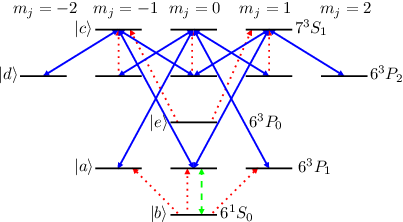
Following [15], we introduce the full coupling scheme (Fig. 3) for all relevant two-electron states of mercury [30] including an additional trapping state . These 13 states can be classified by the Zeeman manifolds
| (11) | ||||
| (12) | ||||
| (13) | ||||
| (14) | ||||
| (15) |
The atomic states are labeled as with the principal quantum number , the total angular momentum quantum number , and the projection quantum number .
To prevent population trapping in , a repump field
| (16) |
is introduced with a detuning . Further, an incoherent pump rate on the transitions between and prevents population trapping in .
Using a convenient interaction picture, the system’s Hamiltonian in dipole and rotating wave approximation is given by
| (17) | ||||
| (18) | ||||
The projection operators are defined as
| (19) |
while the lowering operators are given by
| (20) | ||||
employing Wigner 3-j symbols [30] and the spherical polarization vectors , . The Rabi frequencies polarization components are given by
| (21) | ||||||
| (22) |
with being the transition’s reduced dipole matrix element [30]. Experimental values have been taken from the NIST database [31] and are summarized in Table 1.
| Transition | (nm) | (MHz) | () |
|---|---|---|---|
The laser fields’ polarization vectors are given by
| (23) |
The system’s Bloch equations generalize Eq. (5) by summing over all polarizations and allowed transitions.
IV Doppler broadening
Doppler broadening is the main obstacle for LWI at short wavelengths. This becomes increasingly problematic if drive and probe field’s frequencies differ strongly [6], as is the case in the discussed scheme. To overcome this problem, [15] proposes a Doppler-free three-photon transition. A particle moving at the velocity relative to the emitter of the electromagnetic wave with angular frequency and wave vector experiences a linear Doppler shifted frequency . Therefore, a moving atom senses the Doppler-shifted three-photon detuning
| (24) |
If the fields satisfy the three-photon resonance for an atom at rest, i. e., , then this is true for every velocity group by choosing , as shown in Fig. 4.

The resulting velocity averaged linear susceptibility is defined by the Doppler distribution
| (25) |
at the temperature with the atomic mass of mercury and the Boltzmann constant .
In Fig. 5 (a), the central narrow feature of LWI for atoms at rest is shown (cf. Fig. 2). At finite temperature, this gain peak persists even though at reduced magnitude, see Fig. 5 (b). Both spectra are approximately Lorentzian with a width (FWHM) of kHz (a) and kHz (b). As a comparison, the probe transition’s Doppler width (FWHM) for a temperature of K is GHz.

V Other broadening mechanisms
In this section, we discuss further broadening mechanisms that may affect the performance of LWI and estimate their influence on the considered system for realistic experimental conditions.
For the atomic density and temperature under consideration (cf. Sec. III), we estimate the ratio of dephasing rate to radiative coherence decay rate [23, 24, 25, 26] to , , and . The collisional dephasing rates of all other coherences are considerably smaller than these [24]. Therefore, we neglect collisional line broadening in our calculations. The coherence is of special importance since it is closely connected to the aforementioned three-photon transition. We neglect its dephasing rate assuming that it is considerably smaller than the coherence decay induced by the technical noise of the driving lasers we elaborate on later.
Further, we estimate the frequency shift induced by the recoil an atom exhibits during absorbing or emitting a photon [27, 28]. For the lasing transition this shift is kHz, with the atomic mass of mercury u and the speed of light . For the other relevant transitions this shift is even smaller. The results of realistic calculations of the gain peak, presented later in this paper, show a width more than an order of magnitude larger than this shift. Therefore, we neglect the effect of recoil shifts in our calculations. However, it is worth mentioning that for possible generalizations of the discussed scheme towards shorter wavelength recoil effects may need to be considered.
VI Technical noise of driving fields
To implement the driving laser fields and , we plan to utilize single mode external cavity diode lasers, which exhibit predominately phase diffusion [32, 33] with linewidths below MHz. Further, the repump field will be implemented as a spectrally broadened laser with a linewidth of MHz. Clearly, technical fluctuations in the phase affect coherent multi-photon processes negatively. Therefore, we will investigate the influence of phase noise on the LWI system’s gain in this section. The influence of phase noise on the absorption spectra has been discussed for two-level atoms [32, 34, 35] and three-level LWI schemes [36, 37, 38, 39]. A lucid introduction to stochastic methods can be found in [40, 41].
We start by writing the complex amplitudes of the slowly varying driving fields (cf. Eq. (1)) as
| (26) |
with the deterministic amplitude , the stochastic phase , and .
The phases are modeled as stochastic processes undergoing diffusion characterized by a linewidth satisfying the stochastic Ito differential equations
| (27) |
with being a standard Wiener process [40] with a vanishing mean and variance . Therefore, the probability density function satisfies the pure diffusion Fokker-Planck equation
| (28) |
The stochastic average of a quantity with respect to the stochastic phases is given by
| (29) |
It is worth to note the difference between this stochastic average, the quantum mechanical average, and the Doppler average. Throughout this paper will always denote the stochastic average over the phase fluctuations. This stochastic phase-diffusion model (PDM) leads to a stationary field autocorrelation function
| (30) |
and a Lorentzian spectrum with linewidth .
The Bloch equations depend functionally on the stochastic driving fields, therefore they become stochastic differential equations as well. Applying the rules of stochastic Ito calculus, one can derive ordinary differential equations for the stochastic averaged Bloch equations (cf. Appendix A).
The physical observables are stochastic averaged populations and contributions to the dipole energy . Therefore, it is useful to introduce a unitary transformation of the stochastic density operator
| (31) |
that gauges away the stochastic phases. The resulting equations of motion for the averaged density operator over the driving fields’ phase fluctuations are given by
| (32) |
The full expression of the phase diffusion Liouvillian can be found in the Appendix A. It contains additional damping terms for the atomic coherences depending on the fields’ linewidths.
In Fig. 6 the resulting Doppler averaged absorption spectra calculated from Eq. (32) are shown for different linewidths.

The gain peak of the calculated absorption spectra shows a strong dependency on the driving fields’ linewidths. While its width increases with increasing linewidths, its magnitude decreases.
The dependency of the susceptibility’s imaginary part at resonance on the driving fields’ linewidths is shown in Fig. 7 for different temperatures. For increasing temperatures in the vapor cell the atomic density and with it the linear gain increases. However, this comes at the cost of increasing collisional dephasing rates that affect the atomic coherence used for LWI. By neglecting these rates we are not able to determine the optimal density at which the trade-off between optical depth and collisional dephasing maximizes the gain. This has to be determined experimentally.
Fig. 8 shows the dependency of the linear gain on the strength of the incoherent pump applied to the probe transition for different linewidths. This result shows that the loss in linear gain caused by phase noise can to some extent be compensated by stronger pumping on the probe transition.


VII Expected laser power
In the previous sections the gain medium’s linear response to the external probe field was investigated, whereas in this section the field will be treated as a dynamical quantity, the lasing field. By applying semiclassical laser theory [42, 43, 44, 45] this will lead to the stationary laser power.
The dynamics of the lasing field is determined by the Maxwell equations from which the wave equation
| (33) |
can be deduced under the assumptions that the charge density, the gradient of , and the magnetization vanish and the current density is given by conductivity times the electric field . The polarization density couples this wave equation to the medium’s Bloch equations.
To solve this problem, we start by expanding the laser field
| (34) |
in the resonator’s Hermite-Gauss modes (cf. Appendix B) that are known to accurately describe modes in ordinary optical resonators [46]. is the phase and is the real amplitude of the -th mode. Choosing a convenient normalization, the Hermite-Gauss modes obey the orthogonality relation
| (35) |
with being the resonator’s mode volume. The next step is to project Eq. (33) onto by using Eqs. (1), (34), and (35). If we assume the paraxial approximation to be valid, small losses in the resonator and further apply the slowly varying envelope approximation (SVEA), we obtain the equation of motion for the th mode amplitude
| (36) |
with
| (37) | ||||
| (38) |
and denoting the volume of the gain medium. In the derivation of Eq. (36), we used the dispersion relation for the wave vector of the Hermite-Gauss modes and the fact that these modes approximately obey the Helmholtz equation (cf. Appendix B). In the following we will assume that the amplitude of the TEM00 is much larger than all higher amplitudes with . Consequently, these higher amplitudes will be neglected. For convenience we drop the index .
In order to solve Eq. (36), the dependency of the medium’s polarization amplitude on the amplitude of the laser field needs to be known. This dependency is determined by the Bloch equations averaged over the Maxwell-Boltzmann distribution and the phase fluctuations exhibited by the external fields. As we are interested in the stationary limit, we expand the medium’s polarization density in powers of the lasing field with the instantaneous (non-)linear susceptibilities using the ansatz
| (39) |
These susceptibilities are averaged over the driving fields’ phase fluctuations and the Maxwell-Boltzmann velocity distribution and are assumed to be homogeneous over the laser modes spatial extension in the medium. This assumption will be rectified in the next section. It is worth noting that for Eq. (39) we assumed frequency conversion effects to be negligible. Furthermore, the usage of instantaneous susceptibilities causes Eq. (39) to be only valid if varies slowly compared to the time it takes for the medium to respond. Using the expansion given in Eq. (39), the polarization amplitude can be written as
| (40) | ||||
| (41) |
with and
| (42) | ||||
| (43) |
We calculate the expansion parameter of Eq. (41) by fitting a polynomial of degree to the numerical calculated . A coefficient comparison between Eqs. (40) and (41) then yields the nonlinear susceptibilities. Our calculations show a truncation with to be sufficient. We introduce the photon number as . Inserting Eq. (40) in Eq. (36) and truncating the series at , we arrive at
| (44) |
with the linear gain parameter
| (45) |
the nonlinear saturation parameters
| (46) |
and . Thus, the stationary photon number is given
| (47) |
The sign of the linear gain parameter indicates if the laser system is above () or below () threshold, while and are saturation parameters that determine the stationary power when above threshold. For , we obtain the standard form of the photon number equation for a laser [44].
Assuming the laser mode to be transversely well localized in the medium, the approximation is justified. Further, the stationary laser power can be calculated to with being the mode’s beam waist. Fig. 9 shows the dependency of the calculated stationary laser power on the pumping power for different linewidths of the driving fields. The pumping power is related to the incoherent pump rate by
| (48) |
We assume the pump field to have a Gaussian spectrum with central frequency and variance MHz corresponding to a Doppler spectrum at temperature K. Further, denotes the effective area cross-section of the pump field’s beam. The graphs show the expected behavior, no lasing until a threshold pump power and a merely linear dependency on the pump power above threshold. Increasing linewidths shift the threshold towards larger pump intensities and result in a flatter slope.
Fig. 10 shows the dependency of the threshold pump power on the driving fields’ linewidths. This graph reveals the importance of reducing the phase noise of the external laser for the feasibility of this experiment.


VIII Resonator modes
In the previous section, it has been assumed that the spatial distribution of the laser field is that of a Gaussian mode. In this section this assumption’s validity will be proved by calculating the spatial gain distribution in the medium. Using this result, we obtain the real modes of the laser system. Assuming the laser field to be highly monochromatic, we can neglect the time dependency of its amplitude and write
| (49) |
In the paraxial approximation, we assume that and are variables and becomes the chronological parameter. Within the linear response approximation the slowly varying envelope obeys the Schrödinger-like wave equation
| (50) |
We have used the following definitions
| (51) | ||||
| (52) |
and the wave vectors norm . It is worth noting that is a non-Hermitian complex potential accounting for changes in the index of refraction and absorption.
VIII.1 Propagation through the empty resonator
Before including the gain medium in our considerations, we will calculate the modes of the empty open resonator. In the following, we will shortly review the basic procedure of light propagation in open cavities [47, 45, 48].
In free space () the solution to Eq. (50) is given by
| (53) |
with the initial field distribution . The explicit form of Eq. (53) for is just the Fresnel diffraction integral and can be evaluated efficiently with fast Fourier transform algorithms.
To simulate the round-trip in an optical resonator the action of a mirror with radii of curvature and and aperture function on the field needs to be specified
| (54) |
Combining free propagation with equal length and the action of the four mirrors in the ring cavity shown in Fig. 11, defines a round trip operator . This yields an eigenvalue problem
| (55) |
for the eigenmodes labeled by the complex eigenvalue . The mirrors have a curvature radius and a tilt angle of . We choose the -direction to be in the sagittal plane and the -direction to be in the tangential plane. From this follows and .

Starting from Fox and Li [49], different methods [46, 50, 51, 52] have been developed to solve this eigenvalue problem. In our work, we use the Arnoldi-Krylov method [53, 54] to find the largest eigenvalues and the corresponding eigenvectors , which are the self-consistent transverse electromagnetic modes (TEM) of the ring cavity defined by . Fig. 12 shows the calculated modes’s intensity patterns on the output mirror. As expected, these modes show strong resemblance to the Hermite-Gauss functions used for the mode expansion in the previous section.

VIII.2 Propagation in inhomogeneous media
In Sec. VII, we have assumed spatially homogeneous susceptibilities to calculate the stationary intensity of the laser field. This does not correspond to the real situation where the intersection of external Gaussian laser beams creates a tilted, ellipsoidal gain distribution as shown in Fig. 13. The orientations of the driving fields’ wave vectors are fixed by the three-photon Doppler free configuration in Fig. 4.
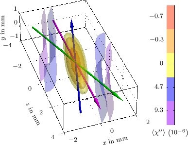
The central yellow/orange structure provides gain for the laser while in the blue structures on both sides amplified absorption is observed. This can be explained by considering the ratio in both areas. The gain region is basically centered around the laser beam associated with resulting in the mentioned ratio to be large, while increased absorption is observed in regions with a small ratio . For small the described coherence effect is not observed since the needed Autler-Townes splitting cannot be achieved whereas a relatively large prevents population trapping in the state and by this means increases absorption on the lasing transition.
To investigate the influence of the inhomogeneous gain distribution on the mode structure, we need to propagate the field through the medium with length
| (56) |
with and . This formal definition of the chronological ordered () propagator is evaluated approximately by splitting the medium into short slices of length and using the split operator method [55, 56]
| (57) |
where we have evaluated the potential at positions .
Now, this modifies the round trip operator of the cavity and the gain medium to
| (58) |
with . The additional factor phenomenologically models the cumulative loss per round trip caused by output coupling and imperfection of optical elements. The corresponding resonator modes can again be calculated using the Arnoldi-Krylov method.
VIII.3 Results
The crucial parameters for the experiment are the gain per round-trip and the beam quality that can be measured by the parameter [57, 58] defined for the transverse -direction as
| (59) |
with the wavelength , the divergence angle in -direction , and beam diameter in -direction at the beam’s waist. Hermite-Gauss modes of order have a beam quality characterized by .
The most important control parameter for the gain medium’s structure are the spatial field distributions of the driving lasers. We assume the driving fields to be Gaussian beams focussed in the center of the gain medium. Consequently, the field distributions are determined by the beams’ waists. Since the driving fields’ peak intensity is constrained to have optimal gain in the focal region, a certain beam waist corresponds to a certain power required.
Figs. 14 and 15 show the dependencies of the linear amplification per round-trip and the beam quality parameter on the driving fields’ waist respectively. For small the laser field is attenuated in the medium, resulting in , whereas for larger the gain region increases and at some point the gain in the medium compensates for the absorption and diffraction losses (); for yet larger the field is amplified after each round-trip and the laser process starts. If is much larger than the laser field’s extension in the gain medium, the gain saturates. In the case of large the beam quality of the laser field reaches the beam quality of the empty resonator modes (cf. Fig. 12). For small the beam quality is worse, exceeds the former mentioned value considerably. This can be explained by interpreting the gain region in the medium as an effective aperture for the laser beam. If this aperture is much larger than the transverse extension of the laser beam’s intensity distribution, the aperture has no significant influence on the laser beam and the resulting modes are those of the empty resonator. For smaller the effective aperture of the gain region becomes smaller and the laser beam is diffracted at this aperture, resulting in poorer beam quality and larger values. In the intermediate regime one observes an minimum in , optimal mode quality. This is obtained when the gain structure in the medium and the respective mode’s intensity distribution match best. Diffraction patterns in the outer regions of the intensity distributions are absorbed while the relevant part of the mode is not diffracted.


IX Conclusions
We have developed a realistic multi-level model for the UV lasing scheme in mercury vapor proposed in [15], including technical noise of the driving field, Doppler broadening, the spatial inhomogeneous structure of the gain medium, and self-consistent eigenmodes of a four-mirror ring cavity. This model was used to identify crucial experimental parameters such as the linewidths and the waists of the driving fields and to investigate the dependency of linear gain, stationary power, and mode quality of the laser system on these parameters. The results of this analysis demonstrate the parameter ranges and the expected performance of the laser system.
Acknowledgments
We acknowledge support by the Deutsche Forschungsgemeinschaft (DFG) grant WA 1658/2-1.
Appendix A Details of PDM calculation
The stochastic phases , , and appear in the Bloch equations as parameters. To separate the stochastic and deterministic dynamics, we apply the transformation given in Eq. (31) with
| (60) | ||||
| (61) |
The sum over extends over the atomic states whereas . Applying the rules of Ito calculus [40] on the variable substitution , we obtain
| (62) |
with . It is worth noting that is deterministic as the transformation separated the deterministic evolution from the stochastic fluctuations. Under the assumption that is non-anticipating , the average of Eq. (62) over the phase fluctuations is given by
| (63) |
The phase-diffusion Liouvillian appearing in Eq. (32) is thus given by
| (64) |
For Eq. (63) the equations (27) for the stochastic phases were used together with the properties of the independent Wiener increments .
Appendix B Hermite-Gauss modes
The Hermite-Gauss mode [45] of order is given by
| (65) |
with the one-dimensional mode function
| (66) |
the normalization factor , the Guoy phase , the beam width , and the curvature radius . denotes the -th Hermite polynomial. In the case of the ring resonator it is important to note that the -direction is the direction of the optical axis tilted by the mirrors and that the - and -direction are the corresponding local transverse directions.
The Hermite-Gauss modes are solutions to the paraxial wave equation in vacuum (cf. Eq. (50)). In the paraxial case they approximately obey the Helmholtz equation
| (67) |
References
- [1] O. Kocharovskaya and Y. Khanin, “Coherent amplification of an ultrashort pulse in a three-level medium without population inversion,” JETP Lett. 48, 630 (1988).
- [2] S. E. Harris, “Lasers without inversion: Interference of lifetime-broadened resonances,” Phys. Rev. Lett. 62, 1033–1036 (1989).
- [3] M. O. Scully, S.-Y. Zhu, and A. Gavrielides, “Degenerate quantum-beat laser: Lasing without inversion and inversion without lasing,” Phys. Rev. Lett. 62, 2813–2816 (1989).
- [4] O. Kocharovskaya, “Amplification and lasing without inversion,” Physics Reports 219, 175 – 190 (1992).
- [5] M. O. Scully and M. Fleischhauer, “Lasers without inversion,” Science 263, 337 (1994).
- [6] M. D. Lukin, M. O. Scully, G. R. Welch, E. S. Fry, L. Hollberg, G. G. Padmabandu, H. G. Robinson, and A. S. Zibrov, “Lasing without inversion: the road to new short-wavelength lasers,” Laser Physics 6, 436–447 (1996).
- [7] J. Mompart and R. Corbalán, “Lasing without inversion,” Journal of Optics B: Quantum and Semiclassical Optics 2, R7 (2000).
- [8] A. Nottelmann, C. Peters, and W. Lange, “Inversionless amplification of picosecond pulses due to zeeman coherence,” Phys. Rev. Lett. 70, 1783–1786 (1993).
- [9] E. S. Fry, X. Li, D. Nikonov, G. G. Padmabandu, M. O. Scully, A. V. Smith, F. K. Tittel, C. Wang, S. R. Wilkinson, and S.-Y. Zhu, “Atomic coherence effects within the sodium line: Lasing without inversion via population trapping,” Phys. Rev. Lett. 70, 3235–3238 (1993).
- [10] A. S. Zibrov, M. D. Lukin, D. E. Nikonov, L. Hollberg, M. O. Scully, V. L. Velichansky, and H. G. Robinson, “Experimental demonstration of laser oscillation without population inversion via quantum interference in rb,” Phys. Rev. Lett. 75, 1499–1502 (1995).
- [11] J. A. Kleinfeld and A. D. Streater, “Gain and coherence effects induced by strong cw-laser coupling in potassium˘rare-gas mixtures,” Phys. Rev. A 53, 1839–1853 (1996).
- [12] S. Y. Kilin, K. T. Kapale, and M. O. Scully, “Lasing without inversion: Counterintuitive population dynamics in the transient regime,” Phys. Rev. Lett. 100, 173601 (2008).
- [13] A. A. Svidzinsky, L. Yuan, and M. O. Scully, “Transient lasing without inversion,” New Journal of Physics 15, 053044 (2013).
- [14] L. Yuan, D. Wang, A. A. Svidzinsky, H. Xia, O. Kocharovskaya, A. Sokolov, G. R. Welch, S. Suckewer, and M. O. Scully, “Transient lasing without inversion via forbidden and virtual transitions,” Phys. Rev. A 89, 013814 (2014).
- [15] E. S. Fry, M. D. Lukin, T. Walther, and G. R. Welch, “Four-level atomic coherence and cw vuv lasers,” Optics Communications 179, 499 – 504 (2000).
- [16] M. D. Lukin, S. F. Yelin, M. Fleischhauer, and M. O. Scully, “Quantum interference effects induced by interacting dark resonances,” Phys. Rev. A 60, 3225–3228 (1999).
- [17] M. Takeoka, T. Nakata, and F. Kannari, “Low-threshold amplification of vacuum-ultraviolet radiation in bichromatically driven Kr gases,” J. Opt. Soc. Am. B 15, 2967–2974 (1998).
- [18] W. P. Schleich, Quantum Optics in Phase Space (Wiley, 2001).
- [19] S. M. Barnett and P. M. Radmore, Methods in Theoretical Quantum Optics (Oxford University Press, 1997).
- [20] W. H. Louisell, Quantum Statistical Properties of Radiation (Wiley, 1973).
- [21] A. Roth, Vacuum Technology (North-Holland, 1990).
- [22] P. Villwock, “Kühlen und Fangen von neutralen Hg-Atomen,” Ph.D. thesis, TU Darmstadt (2010).
- [23] E. Lewis, “Collisional relaxation of atomic excited states, line broadening and interatomic interactions,” Physics Reports 58, 1 – 71 (1980).
- [24] T. Beyer, D. Kolbe, M. Scheid, F. Markert, and J. Walz, “Two-photon spectroscopy of mercury and velocity-selective double resonances,” Phys. Rev. A 80, 053414 (2009).
- [25] P. Laporte and H. Damany, “High density self-broadening of the 253.65 nm mercury resonance line,” Journal of Quantitative Spectroscopy and Radiative Transfer 22, 447 – 466 (1979).
- [26] C. O’Brien, P. M. Anisimov, Y. Rostovtsev, and O. Kocharovskaya, “Coherent control of refractive index in far-detuned systems,” Phys. Rev. A 84, 063835 (2011).
- [27] J. Guo, P. R. Berman, B. Dubetsky, and G. Grynberg, “Recoil-induced resonances in nonlinear spectroscopy,” Phys. Rev. A 46, 1426–1437 (1992).
- [28] P. Horak, K. M. Gheri, and H. Ritsch, “Recoil-induced lasing of cold atoms,” Phys. Rev. A 52, 554–565 (1995).
- [29] R. Kubo, “Statistical-Mechanical Theory of Irreversible Processes. I. General Theory and Simple Applications to Magnetic and Conduction Problems,” Journal of the Physical Society of Japan 12, 570–586 (1957).
- [30] I. I. Sobelman, Atomic Spectra and Radiative Transitions (Springer, 1991), 2nd ed.
- [31] National Institute of Standards and Technology, “Atomic Spectra Database,” (2013). Http://www.nist.gov/pml/data/asd.cfm.
- [32] T. Haslwanter, H. Ritsch, J. Cooper, and P. Zoller, “Laser-noise-induced population fluctuations in two- and three-level systems,” Phys. Rev. A 38, 5652–5659 (1988).
- [33] M. Osinski and J. Buus, “Linewidth broadening factor in semiconductor lasers–an overview,” Quantum Electronics, IEEE Journal of 23, 9–29 (1987).
- [34] H. Ritsch, P. Zoller, and J. Cooper, “Power spectra and variance of laser-noise-induced population fluctuations in two-level atoms,” Phys. Rev. A 41, 2653–2667 (1990).
- [35] R. Walser and P. Zoller, “Laser-noise-induced polarization fluctuations as a spectroscopic tool,” Phys. Rev. A 49, 5067–5077 (1994).
- [36] M. Fleischhauer, M. D. Lukin, D. E. Nikonov, and M. O. Scully, “Influence of pump-field phase diffusion on laser gain in a double- non-inversion laser,” Optics Communications 110, 351 – 357 (1994).
- [37] S.-q. Gong, Z.-z. Xu, Z.-q. Zhang, and S.-h. Pan, “Change from an inversion laser to a noninversion laser due to a phase-fluctuation effect,” Phys. Rev. A 52, 4787–4790 (1995).
- [38] G. Vemuri and D. M. Wood, “Lasing without inversion with a fluctuating pump: Gain dependence on pump noise and frequency,” Phys. Rev. A 50, 747–753 (1994).
- [39] S. Sultana and M. S. Zubairy, “Effect of finite bandwidth on refractive-index enhancement and lasing without inversion,” Phys. Rev. A 49, 438–448 (1994).
- [40] C. W. Gardiner, Handbook of Stochastic Methods, Springer series in synergetics (Springer, 2003), 3rd ed.
- [41] N. G. van Kampen, Stochastic Processes in Physics and Chemistry (North-Holland, 1981).
- [42] W. E. Lamb, “Theory of an optical maser,” Phys. Rev. 134, A1429–A1450 (1964).
- [43] M. Sargent, M. O. Scully, and W. E. Lamb, Laser Physics (Addison-Wesley Publishing Company, 1974).
- [44] H. Haken, Light, vol. 2 (North-Holland, 1985).
- [45] A. Siegman, Lasers (University Science Books, 1986).
- [46] A. E. Siegman and H. Y. Miller, “Unstable optical resonator loss calculations using the prony method,” Appl. Opt. 9, 2729–2736 (1970).
- [47] M. Born and E. Wolf, Principles of Optics (Pergamon Press, 1959).
- [48] N. Hodgson and H. Weber, Laser Resonators and Beam Propagation (Springer, 2004), 2nd ed.
- [49] A. G. Fox and T. Li, “Resonant modes in a maser interferometer,” Bell System Technical Journal 40, 453–488 (1960).
- [50] W. H. Southwell, “Virtual-source theory of unstable resonator modes,” Opt. Lett. 6, 487–489 (1981).
- [51] C. Yuanying, W. Youqing, H. Jin, and L. Jiarong, “An eigenvector method for optical field simulation,” Optics Communications 234, 1 – 6 (2004).
- [52] G. New and Z. D. Kaddour, “Unstable resonator modes: a beam expansion approach,” Journal of Modern Optics 59, 1363–1370 (2012).
- [53] W. P. Latham and G. C. Dente, “Matrix methods for bare resonator eigenvalue analysis,” Appl. Opt. 19, 1618–1621 (1980).
- [54] G. H. Golub and C. F. van Loan, Matrix Computations (The Johns Hopkins University Press, 1996).
- [55] J. Fleck, J.A., J. Morris, and M. Feit, “Time-dependent propagation of high energy laser beams through the atmosphere,” Applied physics 10, 129–160 (1976).
- [56] J. van Roey, J. van der Donk, and P. E. Lagasse, “Beam-propagation method: analysis and assessment,” J. Opt. Soc. Am. 71, 803–810 (1981).
- [57] A. E. Siegman, “Defining, measuring, and optimizing laser beam quality,” Proc. SPIE 1868, 2–12 (1993).
- [58] Technical Committee ISO/TC 172, Optics and photonics, Subcommittee SC 9, Electro-optical systems, “Lasers and laser-related equipment — test methods for laser beam widths, divergence angles and beam propagation ratios,” Tech. Rep. ISO 11146-1:2005(E), International Organization for Standardization (2005).