Projection Algorithms for Nonconvex Minimization with Application to Sparse Principal Component Analysis Thanks: Author names are ordered alphabetically. March 28, 2015, revised December 25, 2015.The authors gratefully acknowledge support by National Science Foundation under grants 1115568 and 1522629 and by Office of Naval Research under grants N00014-11-1-0068 and N00014-15-1-2048.
Abstract
We consider concave minimization problems over nonconvex sets. Optimization problems with this structure arise in sparse principal component analysis. We analyze both a gradient projection algorithm and an approximate Newton algorithm where the Hessian approximation is a multiple of the identity. Convergence results are established. In numerical experiments arising in sparse principal component analysis, it is seen that the performance of the gradient projection algorithm is very similar to that of the truncated power method and the generalized power method. In some cases, the approximate Newton algorithm with a Barzilai-Borwein (BB) Hessian approximation and a nonmonotone line search can be substantially faster than the other algorithms, and can converge to a better solution.
keywords
sparse principal component analysis, gradient projection, nonconvex minimization, approximate Newton, Barzilai-Borwein method1 Introduction
Principal component analysis (PCA) is an extremely popular tool in engineering and statistical analysis. It amounts to computing the singular vectors associated with the largest singular values. In its simplest setting, the rank-one approximation, amounts to solving an optimization problem of the form
| (1) |
where is the covariance matrix associated with the data matrix and is the Euclidean norm. As pointed out in [26], there is no loss of generality in assuming that is positive definite since
whenever is feasible in (1).
The lack of interpretability has been a major concern in PCA. Sparse PCA partly addresses this problem by constraining the number of nonzero components of the maximizing in (1). Given a positive integer , the sparse PCA problem associated with (1) is
| (2) |
where denotes the number of nonzero components of . Due to the sparsity constraint in (2), the feasible set is no longer convex, which makes the optimization problem more difficult.
A large quantity of literatures focus on using the sparsity norms, such as the -norm and -norm, in the formulation. Such methods are popular in signal processing and statistics community. Notably, the lasso-related methods appeared in studies such as [9, 13, 12].
In [8] PCA loadings smaller than a certain tolerance are simply set to zero to produce sparse principal components. More recently, optimization-based approaches have been used to introduce sparsity. For example, in [25] sparsity is achieved using an relaxation. That is, the problem (2) is replaced by
| (3) |
where . The solution of the relaxed problem (3) yields an upper bound for the solution of (2). In [21] the Rayleigh quotient problem subject to an -constraint is successively maximized using the authors’ SCoTLASS algorithm. In [33], the authors formulate a regression problem and propose numerical algorithms to solve it. Their approach can be applied to large-scale data, but it is computationally expensive. In [11] a new semi-definite relaxation is formulated and a greedy algorithm is developed that computes a full set of good solutions for the target number of non-zero coefficients. With total complexity , the algorithm is computationally expensive. Other references related to sparse optimization include [10, 17, 18, 20, 24, 29].
Our work is largely motivated by [22], [26], and [32]. In [22] both -penalized and -penalized sparse PCA problems are considered and a generalized power method is developed. The numerical experiments show that their approach outperforms earlier algorithms both in solution quality and in computational speed. Recently, [26] and [32] both consider the -constrained sparse PCA problem and propose an efficient truncated power method. Their algorithms are equivalent and originated from the classic Frank-Wolfe [14] conditional gradient algorithm.
In this paper, we study both the gradient projection algorithm and an approximate Newton algorithm. Convergence results are established and numerical experiments are given for sparse PCA problems of the form (2). The algorithms have the same iteration complexity as the fastest current algorithms, such as the algorithms proposed in [22], [26] and [32], which is in solving problem (2). The gradient projection algorithm with unit step size has nearly identical performance as that of the conditionl gradient algorithm with unit step-size (ConGradU) [26] and the truncated power method (Tpower) [32]. On the other hand, the approximate Newton algorithm can often converge faster to a better objective value than the other algorithms.
The paper is organized as follows. In Section 2 we analyze the gradient projection algorithm when the constraint set is nonconvex. Section 3 introduces and analyzes the approximate Newton scheme. Section 4 examines the performance of the algorithms in some numerical experiments based on classic examples found in the sparse PCA literature.
Notation. If is differentiable, then denotes the gradient of , a row vector, while denotes the gradient of arranged as a column vector. The subscript denotes the iteration number. In particular, is the -th -iterate and . The -th element of the -th iterate is denoted . The Euclidean norm is denoted , while denotes cardinality (number of non-zero elements). If , then the support of is the set of indices of nonzeros components:
If , then is the convex hull of . If , then is the vector obtained by replacing for by 0. If is a set, then is its complement.
2 Gradient projection algorithm
Let us consider an optimization problem of the form
| (4) |
where is a nonempty, closed set and is differentiable on . Often, the gradient projection algorithm is presented in the context of an optimization problem where the feasible set is convex [3, 4, 16]. Since the feasible set for the sparse PCA problem (2) is nonconvex, we will study the gradient projection algorithm for a potentially nonconvex feasible set .
The projection of onto is defined by
For the constraint set that arises in sparse PCA, the projection can be expressed as follows:
Proposition 1.
For the set
| (5) |
where is a positive integer, we have
where is the vector obtained from by replacing elements of with smallest magnitude by .
Proof.
If , then . Hence, we have
| (6) |
In [26, Prop. 4.3], it is shown that the minimum is attained at . We include the proof since it is short and we need to refer to it later. Given any set , the solution of the problem
is by the Schwarz inequality, and the corresponding objective value is , where is the vector obtained by replacing for by 0. Clearly, the minimum is attained when is the set of indices of associated with the absolute largest components. ∎
In general, when is closed, the projection exists, although it may not be unique when is nonconvex. If is the current iterate, then in one of the standard implementations of gradient projection algorithm, is obtained by a line search along the line segment connecting and , where is the gradient at and is the step size. When is nonconvex, this line segment is not always contained in . Hence, we will focus on gradient projection algorithms of the form
| (7) |
Since is closed, exists for each . We first observe that always forms an obtuse angle with the gradient, which guarantees descent when is concave.
Lemma 2.
If , then
| (8) |
In particular, for this gives
| (9) |
If is concave over conv, then .
Proof.
The following result is well known.
Proposition 3.
If is concave and , then
| (12) |
where the first infimum is attained only when the second infimum is attained. Moreover, if is differentiable at , then
| (13) |
Proof.
Remark 1.
Note that at a local minimizer of over a nonconvex set , the inequality may not hold for all . For example, suppose that where has the direction shown in Figure 1. The point A is a local minimizer of over , but (13) does not hold. Hence, Proposition 3 is only valid for a global minimizer, as stated.

Next, we consider the special choice in Proposition 3.
Corollary 4.
If is concave and
then
| (14) |
whenever for some .
Proof.
The following property for the projection is needed in the main theorem:
Lemma 5.
If is a nonempty closed set, is a sequence converging to and is a sequence converging to , then .
Proof.
Since for each and is closed, . Hence, we have
If this inequality is an equality, then we are done; consequently, let us suppose that
As tends to , the right side approaches , which yields a contradiction. ∎
We now give further justification for the convergence of the gradient projection algorithm in the nonconvex setting.
Theorem 6.
If is concave, is a compact nonempty set, and is generated by the gradient projection algorithm , then we have for each and
| (15) |
If is the limit of any convergent subsequence of the and the step size approaches a limit , then
| (16) |
If is continuously differentiable around , then
| (17) |
for some .
Proof.
Sum the concavity inequality (11) for to obtain
| (18) |
Since is continuous and is compact, is finite and
| (19) |
Together, (18) and (19) yield (15) since for each by Lemma 2.
The relation (16) is (8) with replaced by . For convenience, let also denote the subsequence of the iterates that converges to , and let denote the iterate produced by . Since lies in a compact set, there exists a subsequence converging to a limit . Again, for convenience, let and denote this convergent subsequence. By (15) and the fact that is continuously differentiable around , we have
By Lemma 5, . ∎
.
When is convex, much stronger convergence results can be established for the gradient projection algorithm. In this case, the projection onto is unique. By [16, Prop. 2.1], for any and , if and only if is a stationary point for (4). That is,
Moreover, when is convex,
| (20) |
for any and . Hence, (17) implies that the left side of (20) vanishes at , which means that . And conversely, if , then (17) holds.
3 Approximate Newton algorithm
To account for second-order information, Bertsekas [4] analyzes the following version of the gradient projection method:
Strong convergence results can be established when is convex and is strongly convex. On the other hand, if is concave, local minimizers are extreme points of the feasible set, so the analysis is quite different. Suppose that is approximated by a multiple of the identity matrix as is done in the BB method [2]. This leads to the approximation
| (21) |
Let us consider the algorithm in which the new iterate is obtained by optimizing the quadratic model:
| (22) |
After completing the square, the iteration is equivalent to
If , then this reduces to ; in other words, perform the gradient projection algorithm with step size . If , then the iteration reduces to
| (23) |
where
| (24) |
If is unbounded, then this iteration does not make sense since the maximum occurs at infinity. But if is compact, then the iteration is justified in the sense that the projection (24) exists and the iteration is based on a quadratic model of the function, which could be better than a linear model.
Suppose that for some . Due to the equivalence between (22) and (23), it follows that
| (25) |
That is, is a global optimizer of the quadratic objective in (25) over . Since the objective in the optimization problem (25) is concave, Proposition 3 yields
| (26) |
Hence, fixed points of the iteration (23) satisfy the necessary condition (26) associated with a global optimum of (4).
In the special case where is the constraint set (5) appearing in sparse PCA and , the maximization in (24) can be evaluated as follows:
Proposition 7.
For the set in associated with sparse PCA, we have
Proof.
As in the proof of Proposition 1, when lies in the set of (5). Hence, we have
Given any set , the solution of the problem
is by the Schwarz inequality, and the corresponding objective value is . Clearly, the maximum is attained when corresponds to a set of indices of associated with the absolute largest components. ∎
Let us now study the convergence of the iterates generated by the quadratic model (22). The case where corresponds to the gradient projection algorithm which was studied in Section 2. In this section, we focus on and the iteration . For the numerical experiments, we employ a BB-approximation [2] to the Hessian given by
| (27) |
It is well known that the BB-approximation performs much better when it is embedded in a nonmonotone line search. This leads us to study a scheme based on the GLL stepsize rule of [15]. Let denote the largest of the most recent function values:
Our convention is that when . The nonmonotone approximate Newton algorithm that we analyze is as follows:
| Nonmonotone Approximate Newton (for strongly concave ) | ||||||||||||||
| Given , , and starting guess . | ||||||||||||||
| Set . | ||||||||||||||
|
Note that the approximate Newton algorithm is monotone when the memory . If , then the stepsize acceptance condition in Step 2 is satisfied for and . Hence, when there is no line search. To ensure that lies in the safe-guard interval when using the BB-approximation to the Hessian, it is common to take
where mid denotes median or middle. In the numerical experiments, is large in magnitude and is close to 0, in which case the safe guards have no practical significance; nonetheless, they enter into the convergence theory.
In the approximate Newton algorithm, we make a starting guess for the initial and then increase until the line search acceptance criterion of Step 2 is fulfilled. We first show that for a strongly concave function, the line search criterion is satisfied for sufficiently large, and the stepsize is uniformly bounded away from zero.
Proposition 8.
If is differentiable on a compact set and for some , we have
| (28) |
then Step in the approximate Newton algorithm terminates with a finite , and with bounded away from , uniformly in . In particular, we have .
Proof.
Since is compact, the set is nonempty for each . If , then since is set of elements in farthest from , we have
Rearrange this inequality to obtain
| (29) |
Substitute and in (28) and in (29), and add to obtain
| (30) | |||||
If , then . Hence, by (30), Step 2 must terminate whenever . Since , it follows that Step 2 terminates for a finite . If Step 2 terminates when , then , which implies that . If Step 2 terminates when , then . In either case, . ∎
In analyzing the convergence of the approximate Newton algorithm, we also need to consider the continuity of the operator.
Lemma 9.
If is a nonempty compact set, is a sequence converging to and is a sequence converging to , then .
Proof.
Since for each and is closed, . Hence, we have
If this inequality is an equality, then we are done; consequently, let us suppose that
As tends to , the right side approaches , which yields a contradiction. ∎
The following theorem establishes convergence of the approximate Newton algorithm when is strongly concave.
Theorem 10.
If is continuously differentiable on a compact set and holds for some , then the sequence of objective values generated by the nonmonotone approximate Newton algorithm converge to a limit as tends to infinity. If is any accumulation point of the iterates , then for some , which implies that and hold.
Proof.
By Proposition 8, the stepsize generated by the approximate Newton algorithm satisfies . By the line search criterion and the fact that , , which implies that for all . Since the are monotone decreasing and bounded from below, there exists a limit . Since is continuously differentiable on the compact set , it follows that is uniformly continuous on . Since the stepsize is uniformly bounded away from zero, the same argument used in the proof of [30, Lem. 4] shows that converges to and tends to zero.
Select any satisfying and let be given by
| (31) |
It follows that
| (32) |
Since satisfies (22), we have
| (33) |
Since and approaches zero, we conclude that tends to zero. Hence, if is an accumulation point of the iterates , then is an accumulation point of the . Due to the equivalence between (22) and (23), it follows from (31) that . Since is continuous, is an accumulation point of . By Lemma 9, we have , which completes the proof. ∎
Due to the equivalence between the inclusion and the necessary condition (26) for a global optimum, the change associated with the iteration could be used to assess convergence of the approximate Newton algorithm. That is, if , then satisfies the necessary condition (26) for a global optimizer of (4). As observed in Theorem 10, tends to zero. We now analyze the convergence rate of .
Theorem 11.
If is continuously differentiable on a compact set and holds for some , then there exists a constant , independent of , such that
Proof.
Let denote the index associated with the most recent function values:
In the approximate Newton algorithm, an acceptable step must satisfy the condition
| (34) |
If , then
| (35) |
Since , it follows that , or . During the proof of Theorem 10, we observed that the sequence is monotone decreasing. Consequently, since . Use this inequality and (35) in (34) to obtain
| (36) |
where . Choose and sum the inequality (36) for . We have
| (37) |
where and is the limit of the . Observe that
Combine this relationship with the bound of Proposition 8 and (37) to obtain
This completes the proof. ∎
4 Numerical experiments
We will investigate the performance of the gradient project and approximate Newton algorithm relative to previously developed algorithms in the literature. In our experiments we use the gradient projection algorithm with unit stepsize (GPU):
And in our experiments with the approximate Newton algorithm, we employ the BB approximation (27) for the initial stepsize . The memory is and . This version of the approximate Newton algorithm is denoted GPBB. For the set associated with sparse PCA, we have
We compare the performance of our algorithms to those of both the truncated power method (Tpower) [32] and the generalized power method (Gpower) [22]. The conditional gradient algorithm with unit step-size (ConGradU) proposed in [26] is equivalent to the truncated power method. Both truncated and generalized power method are targeted to the sparse PCA problem (2). The truncated power method handles the sparsity constraint by pushing the absolute smallest components of the iterates to 0. The iteration can be expressed
| (38) |
For comparison, an iteration of the gradient projection algorithm with unit step size GPU is given by
| (39) |
while the approximate Newton algorithm is
| (40) |
where depending on whether , , or respectively. Since the computation of requires the gradient at two points, we start GPBB with one iteration of GPU. For the sparse PCA problem (2), the time for one iteration of any of these methods is basically the time to multiply a vector by the covariance matrix . Note that the monotone approximate Newton algorithm could be more costly since the evaluation of an acceptable may require several evaluations of the objective function.
In the generalized power method, the sparsity constraint is handled using a penalty terms. If denotes the penalty, then Gpower corresponds to the optimization problem
where , while Gpower corresponds to
The parameter needs to be tuned to achieve the desired cardinality; as increases, the cardinality of the Gpower approximation decreases. In contrast, the cardinality is an explicit input parameter for either the truncated power method or for our algorithms; in many applications, cardinality is often specified.
All experiments were conducted using MATLAB on a GNU/Linux computer with 8GB of RAM and an Intel Core i7-2600 processor. For the starting guess in our experiments, we follow the practice of the Tpower algorithm [32] and set , the -th column of the identity matrix, where is the index of the largest diagonal element of the covariance matrix . Our numerical experiments are based on the sparse PCA problem (2). We measure the quality of the solution to (2) computed by any of the methods using the ratio where is the sparse first principal component computed by any of the algorithms for (2) and is the first principal component (a solution of (1)). This ratio is often called the proportion of the explained variance.
Pit props dataset
This dataset [19] contains 180 observations with 13 variables, and a covariance matrix . This is a standard benchmark dataset for Sparse PCA algorithms. We consider or 7, and we adjust the value of to achieve the same sparsity in Gpower. The last column of Table 1 gives the proportion of the explained variance. Observe that all the methods achieve essentially the same proportion of the explained variance.
| Method | Parameters | Explained Variance |
|---|---|---|
| GPBB | ||
| GPBB | ||
| GPU | ||
| GPU | ||
| Tpower(ConGradU) | ||
| Tpower(ConGradU) | ||
| Gpower | () | |
| Gpower | () | |
| Gpower | () | |
| Gpower | () |
We also considered multiple sparse principal components for this data set and got the same results as those obtained in Table 2 of [33] for the Tpower and PathSPCA algorithms. Similarly, for the lymphoma data set [1] and the Ramaswamy data set [27], all methods yielded the same proportion of explained variance, although the value of for Gpower needed to be tuned to achieve the specified cardinality.
Randomly generated data
In the next set of experiments, we consider randomly generated data, where with each entry of generated by a normal distribution with mean 0 and standard deviation 1. For randomly generated matrices, we can study the performance as either or change. Each result that we present is based on an average over 100 randomly generated matrices. In Figure 2 we plot the proportion of the explained variance versus cardinality for and . Observe that GPBB yields a significantly better objective value as the cardinality decreases when compared to either GPU or ConGradU, while GPU and ConGradU have essentially identical performance.

Even though all the algorithms seem to yield similar results in Figure 2 as the cardinality approaches 500, the convergence of the algorithms is quite different. To illustrate this, let us consider the case where the cardinality is 500. In this case where , the sparse PCA problem (2) and the original PCA problem (1) are identical, and the solution of (1) is a normalized eigenvector associated with the largest eigenvalue of . Since the optimal objective value is known, we can compute the relative error
where is the approximation to the optimal objective value generated by any of the algorithms. In Figure 3 we plot the base 10 logarithm of the relative error versus the iteration number. Observe that GPBB is able to reduce the relative error to the machine precision near in about 175 iterations, while ConGradU and GPU have relative error around after 200 iterations. To achieve a relative error around , ConGradU and GPU require about 4500 iterations, roughly 25 times more than GPBB.
Despite the very nonmonotone behavior of the GPBB iterates, the convergence is relatively fast. The results for the explained variance in Figure 2 were obtained by running either ConGradU or GPU for 6000 iterations, while GPBB was run for 200 iterations. Hence, the better objective values obtained by GPBB in Figure 2 were due to the algorithm converging to a better solution, rather than to premature termination of either GPU or ConGradU.

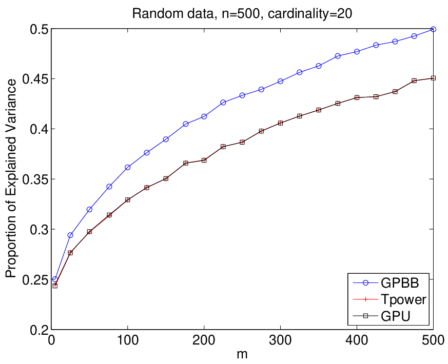
In Figure 4 we plot the proportion of the explained variance versus the iteration number when , , and the cardinality in the random data set. When we plot the function value as in Figure 4, it is more difficult to see the nonmonotone nature of the convergence for GPBB. This nonmonotone nature is clearly visible in Figure 3 where we plot the error instead of the function value. In Figure 5 we show how the explained variance depends on . As increases, the explained variance associated with GPBB becomes much better than that of either ConGradU or GPU.

In Figure 6 we compare the relative error of GPBB for various choices of the memory . Observe that the monotone scheme where is slowest, while gives better performance than that of either a small or where . Note that the running time of the monotone scheme was about 4 times larger than that of the nonmonotone schemes since we may need to test several choices of before generating a successful monotone iterate.

To compare with Gpower, we need to choose a value for . We first consider a simple case and we use the “default” seed in MATLAB to generate this matrix. The algorithms are used to extract the first principal component with , and with tuned to achieve . The results in Table 2 indicate that Gpower performed similar to Tpower, but not as well as GPBB.
| Method | Cardinality | Explained Variance |
|---|---|---|
| GPBB | ||
| Tpower(ConGradU) | ||
| Gpower | () | |
| Gpower | () |
In the next experiment, we consider 100 randomly generated matrices with and , and with the parameter in Gpower chosen to achieve an average cardinality near 100 or 120. As seen in Table 3, Gpower achieves similar values for the proportion of the explained variance as Tpower, while Gpower achieves slightly better results and GPBB achieves the best results.
| Method | Cardinality | Explained Variance |
|---|---|---|
| GPBB | ||
| GPBB | ||
| Tpower(ConGradU) | ||
| Tpower(ConGradU) | ||
| Gpower | (average ) | |
| Gpower | (average ) | |
| Gpower | (average ) | |
| Gpower | (average ) |
Hollywood-2009 dataset, Densest -subgraph (DkS)
Given an undirected graph with vertices and edge set , and given an integer , the densest -subgraph (DkS) problem is to find a set of vertices whose average degree in the subgraph induced by this set is as large as possible. Algorithms for finding DkS are useful tools for analyzing networks. Many techniques have been proposed for solving this problem including [5], [23], [31]. Mathematically, DkS is equivalent to a binary quadratic programming problem
| (41) |
where is the adjacency matrix of the graph; if , while otherwise. We relax the constraints and to and , and consider the following relaxed version of (41)
| (42) |
After a suitable scaling of , this problem reduces to the sparse PCA problem (2).
Let us consider the Hollywood-2009 dataset [6, 7], which is associated with a graph whose vertices are actors in movies, and an edge joins two vertices whenever the associated actors appear in a movie together. The dataset can be downloaded from the following web site:
http://law.di.unimi.it/datasets.php
The adjacency matrix is . In order to apply Gpower to the relaxed problem, we first factored into a product of the form using a Cholesky factorization, where is taken large enough to make positive definite. Here, plays the role of the data matrix. However, one of the steps in the Gpower code updates the data matrix by a rank one matrix, and the rank one matrix caused the updated data matrix to exceed the 200 GB memory on the largest computer readily available for the experiments. Hence, this problem was only solved using Tpower and GPBB. Since the adjacency matrix requires less than 2 GB memory, it easily fit on our 8 GB computer.
In Table 4, we compare the density values obtained by the algorithms. In addition, we also computed the largest eigenvalue of the adjacency matrix , and give the ratio of the density to . Observe that in 2 of the 6 cases, GPBB obtained a significantly better value for the density when compared to Tpower, while in the other 4 cases, both algorithms converged to the same maximum.
| Method | Cardinality | Density | Ratio |
|---|---|---|---|
| GPBB | |||
| GPBB | |||
| GPBB | |||
| GPBB | |||
| GPBB | |||
| GPBB | |||
| Tpower(ConGradU) | |||
| Tpower(ConGradU) | |||
| Tpower(ConGradU) | |||
| Tpower(ConGradU) | |||
| Tpower(ConGradU) | |||
| Tpower(ConGradU) |
5 Conclusion
The gradient projection algorithm was studied in the case where the constraint set may be nonconvex, as it is in sparse principal component analysis. Each iteration of the gradient projection algorithm satisfied the condition . Moreover, if is concave over , then for each . When a subsequence of the iterates converge to , we obtain in Theorem 6 the equality for some where projects a point onto and is the limiting step size. When is convex, is unique and the condition is equivalent to the first-order necessary optimality condition at for a local minimizer.
The approximate Newton algorithm with a positive definite Hessian approximation reduced to the projected gradient algorithm with step size . On the other hand, when , as it is when the objective function is concave and the Hessian approximation is computed by the Barzilai-Borwein formula (27), the iteration amounts to taking a step along the positive gradient, and then moving as far away as possible while staying inside the feasible set. In numerical experiments based on sparse principal component analysis, the gradient projection algorithm with unit step size performed similar to both the truncated power method and the generalized power method. On the other hand, in some cases, the approximate Newton algorithm with a Barzilai-Borwein stepsize and a nonmonotone line search could converge much faster to a better objective function value than the other methods.
References
- [1] A. A. Alizadeh et al., Distinct types of diffuse large b-cell lymphoma identified by gene expression profiling, Nature, 403 (2000), pp. 503–511.
- [2] J. Barzilai and J. M. Borwein, Two point step size gradient methods, IMA J. Numer. Anal., 8 (1988), pp. 141–148.
- [3] Amir Beck and Marc Teboulle, Mirror descent and nonlinear projected subgradient methods for convex optimization, Operations Research Letters, 31 (2003), pp. 167–175.
- [4] D. P. Bertsekas, Projected Newton methods for optimization problems with simple constraints, SIAM J. Control Optim., 20 (1982), pp. 221–246.
- [5] A. Bhaskara, M. Charikar, E. Chlamtac, U. Feige, and A. Vijayaraghavan, Detecting high log-densities: an approximation for densest k-subgraph, in Proceedings of the forty-second ACM symposium on Theory of Computing, ACM, 2010, pp. 201–210.
- [6] Paolo Boldi, Marco Rosa, Massimo Santini, and Sebastiano Vigna, Layered label propagation: A multiresolution coordinate-free ordering for compressing social networks, in Proceedings of the 20th international conference on World Wide Web, ACM Press, 2011.
- [7] Paolo Boldi and Sebastiano Vigna, The WebGraph framework I: Compression techniques, in Proc. of the Thirteenth International World Wide Web Conference (WWW 2004), Manhattan, USA, 2004, ACM Press, pp. 595–601.
- [8] Jorge Cadima and Ian T Jolliffe, Loading and correlations in the interpretation of principle compenents, Journal of Applied Statistics, 22 (1995), pp. 203–214.
- [9] Scott Shaobing Chen, David L Donoho, and Michael A Saunders, Atomic decomposition by basis pursuit, SIAM journal on scientific computing, 20 (1998), pp. 33–61.
- [10] Kenneth L Clarkson, Coresets, sparse greedy approximation, and the Frank-Wolfe algorithm, ACM Transactions on Algorithms (TALG), 6 (2010), p. 63.
- [11] Alexandre d’Aspremont, Francis Bach, and Laurent El Ghaoui, Optimal solutions for sparse principal component analysis, The Journal of Machine Learning Research, 9 (2008), pp. 1269–1294.
- [12] David L Donoho, Compressed sensing, Information Theory, IEEE Transactions on, 52 (2006), pp. 1289–1306.
- [13] Bradley Efron, Trevor Hastie, Iain Johnstone, Robert Tibshirani, et al., Least angle regression, The Annals of statistics, 32 (2004), pp. 407–499.
- [14] M. Frank and P. Wolfe, An algorithm for quadratic programming, Naval Research Logistics Quaterly, 3 (1956), pp. 95–110.
- [15] L. Grippo, F. Lampariello, and S. Lucidi, A nonmonotone line search technique for Newton’s method, SIAM J. Numer. Anal., 23 (1986), pp. 707–716.
- [16] W. W. Hager and H. Zhang, A new active set algorithm for box constrained optimization, SIAM J. Optim., 17 (2006), pp. 526–557.
- [17] E. Hazan and S. Kale, Projection-free online learning, in Proceedings of the 29th International Conference on Machine Learning, J. Langford and J. Pineau, eds., Omnipress, 2012, pp. 521–528.
- [18] Martin Jaggi, Revisiting Frank-Wolfe: Projection-free sparse convex optimization, in Proceedings of the 30th International Conference on Machine Learning, S. Dasgupta and D. McAllester, eds., vol. 28, 2013, pp. 427–435.
- [19] J. Jeffers, Two case studies in the application of principal components, Applied Statistics, 16 (1967), pp. 225–236.
- [20] R. Jenatton, G. Obozinski, and F. Bach, Structured sparse principal component analysis, in International Conference on Artificial Intelligence and Statistics (AISTATS), 2010.
- [21] Ian T Jolliffe, Nickolay T Trendafilov, and Mudassir Uddin, A modified principal component technique based on the LASSO, Journal of Computational and Graphical Statistics, 12 (2003), pp. 531–547.
- [22] Michel Journée, Yurii Nesterov, Peter Richtárik, and Rodolphe Sepulchre, Generalized power method for sparse principal component analysis, The Journal of Machine Learning Research, 11 (2010), pp. 517–553.
- [23] S. Khuller and B. Saha, On finding dense subgraphs, in Automata, Languages and Programming, Springer, 2009, pp. 597–608.
- [24] Simon Lacoste-Julien, Martin Jaggi, Mark Schmidt, and Patrick Pletscher, Block-coordinate Frank-Wolfe optimization for structural SVMs, in Proceedings of the 30th International Conference on Machine Learning, S. Dasgupta and D. McAllester, eds., vol. 28, 2013, pp. 53–61.
- [25] Ronny Luss and Marc Teboulle, Convex approximations to sparse PCA via Lagrangian duality, Operations Research Letters, 39 (2011), pp. 57–61.
- [26] , Conditional gradient algorithms for rank-one matrix approximations with a sparsity constraint, SIAM Review, 55 (2013), pp. 65–98.
- [27] Sridhar Ramaswamy, Pablo Tamayo, Ryan Rifkin, Sayan Mukherjee, Chen-Hsiang Yeang, Michael Angelo, Christine Ladd, Michael Reich, Eva Latulippe, Jill P Mesirov, et al., Multiclass cancer diagnosis using tumor gene expression signatures, Proceedings of the National Academy of Sciences, 98 (2001), pp. 15149–15154.
- [28] R. T. Rockafellar, Convex analysis, Princeton Univ. Press, 1970.
- [29] Bharath K Sriperumbudur, David A Torres, and Gert RG Lanckriet, A majorization-minimization approach to the sparse generalized eigenvalue problem, Machine Learning, 85 (2011), pp. 3–39.
- [30] S. J. Wright, R. D. Nowak, and M. A. T. Figueiredo, Sparse reconstruction by separable approximation, IEEE Trans. Signal Process., 57 (2009), pp. 2479–2493.
- [31] Y. Ye and J. Zhang, Approximation of dense-n/2-subgraph and the complement of min-bisection, Journal of Global Optimization, 25 (2003), pp. 55–73.
- [32] Xiao-Tong Yuan and Tong Zhang, Truncated power method for sparse eigenvalue problems, The Journal of Machine Learning Research, 14 (2013), pp. 899–925.
- [33] Hui Zou, Trevor Hastie, and Robert Tibshirani, Sparse principal component analysis, Journal of Computational and Graphical Statistics, 15 (2006), pp. 265–286.