Unitarization and low-energy scattering data
Abstract
A procedure based on the well known -matrix formalism is presented, which makes patterns in inelastic regions of low-energy scattering data considerably more transparent. It relies on the use of an empirical kernel, obtained by eliminating elastic loops from the experimental amplitude. This allows structures associated with resonances, such as locations, widths and heights, to become visible with the naked eye. The method is illustrated with a study of the -wave amplitude.
pacs
…I introduction
The problem of understanding the dynamical content of mesonic scattering amplitudes, with energies ranging from threshold to a few GeV, is interesting by itself. Nevertheless, it became especially urgent in recent times, because these amplitudes play important roles in final state interactions which occur after primary weak decays of quarks within and mesons. Decays of heavy mesons are presently object of intense scrutiny and the understanding of patterns observed in Dalitz plots require accurate descriptions of both primary weak vertices and hadronic final state interactions[1, 2].
In non-relativistic quantum mechanics, the standard treatment of elastic scattering begins with a potential, which is fed into the Schrödinger equation. In the elastic regime, the potential is real and the dynamical equation yields complex wave-functions, that can be parametrized in terms of phase shifts. When inelasticities are present, one needs a complex optical potential and the corresponding damped wave-functions can be parametrized by their phase shifts and moduli or inelasticity parameters. The formulation of the scattering problem for relativistic particles is roughly similar. Dynamics is now described by the Bethe-Salpeter equation and its kernel corresponds to the potential. In the case of scattering of two generic particles and , this kernel amounts to the sum of all proper intermediate diagrams, that is, those which cannot be split into two pieces by cutting and propagators only. Similarly to what happens with the potential, real kernels give rise to elastic interactions, whereas inelasticities require complex kernels.
In quantum mechanics, the so called inverse problem, in which one attempts to derive potentials from scattering amplitudes, has been widely studied and one knows that it does not have unique solutions. The same holds for the relationship between scattering amplitudes and kernels, in the framework of relativity. This problem has been discussed long ago by Lang[3], who has shown that constraints imposed by unitarity on scattering amplitudes cannot fix kernels completely. However, in the case of low and medium energy meson-meson scattering, the Bethe-Salpeter equation can be simplified and there is a window in which an approximate solution to the inverse problem does exist, which we discuss in the sequence. In the last two decades, this simplification of the Bethe-Salpeter has been extensively used in the dynamical unitarization of amplitudes and successfully applied to a wide number of problems[4, 5].
Quite generally, the reaction is described in terms of Mandelstam variables and, in the center of mass system (CM), results can be expressed in terms of the three-momentum , with ,
| (1) |
The corresponding amplitude can be formally represented in terms of the Bethe-Salpeter equation as
| (2) |
where is the kernel and . This equation can be simplified if one assumes that, at low energies, the dependences of both and on the loop variable can be neglected. This assumption has been used in Ref.[3], tested in many instances[4, 6], and allows the amplitude to be written as
| (3) |
where the function
| (4) |
represents the elastic two-particle propagator, shown in fig.1.

The integral (4) is ultraviolet divergent and a subtraction is needed. Following ref.[7], we write the regular part of as
| (5) |
where the divergent part is contained in . Regularization amounts to replacing this term by an unknown finite constant , which has to be fixed later. The function can be evaluated analytically and, above threshold, one has
| (6) | |||||
| (7) | |||||
with and , the symmetry factor, is 1 for and 2 for . After regularization, eq.(3) may be solved for and one finds[3]
| (8) |
In the elastic regime, the kernel is real and the complex structure of eq.(7) makes automatically unitary. On the other hand, when inelasticities are present, the kernel acquires imaginary components. The conceptual relationship between the amplitude and the kernel can be better understood by rewriting eq.(8) as the geometric series
| (9) | |||||
This shows that the amplitude is just a monotonous iteration of the kernel, as shown in fig.2. It is therefore desirable to know the kernel, since it encompasses all relevant dynamical effects.

Data are usually presented by means of a non-relativistic amplitude , which can be parametrized in terms of either phase and modulus or phase and elasticity, and related with the relativistic amplitude by
| (10) |
Feeding the experimental amplitude , extracted from eq.(10), into eq.(8), and inverting it, one finds a solution to the inverse problem, given by
| (11) |
As we discuss in the sequence, this function conveys dynamical information in a very transparent way, since it is free from intermediate states. It rests at the basis of the procedure proposed here.
In order to evaluate eq.(11), one needs to fix the constant . Since it cannot be fixed directly from data, it must be taken as a free parameter and the function is contaminated by this freedom. However, once a choice is made, the kernel is uniquely determined and its use in eq.(8) yields results which do not depend on conventions. The choice made in Ref.[3] corresponds to . Here, we fix by noting that, at the the point , for which , one has . Using this, together with the result , one finds
| (12) |
One then chooses , because this gives rise to a pole in , correlated with the phase and associated with a light resonance in the channel, of mass .

Bottom: chiral model for , based on a leading contact interaction (C), a bare -channel light resonance and correction terms .
As far as theory is concerned, it is useful to decompose the kernel into light and heavy pieces, denoted by and , as in Fig.3. The latter includes interactions of heavy systems and is discussed in App.B. The light component is real and involves only light-particles. In the framework of chiral models[10], this light kernel is given by the sum of a leading contact term, a light bare -channel resonance , and corrections associated with exchanges of resonances in - and -channels. We stress, however, that the use of a chiral model is not compulsory. The only essential ingredient in is the light resonance, whereas the other terms could well be replaced by a polynomial in , with free coefficients. In order to stress this feature it is convenient to express the light kernel as
| (13) |
Hence the theoretical kernel reads
| (14) |
The form of the bare resonance term is given in App.A and a chiral model for , suited to the system, is presented in App.C.
II amplitude
The preceding discussion, which is somewhat abstract, can be made more concrete with the help of a guiding instance. With this purpose in mind, we present the case of scattering, for which data is available[8] in the range GeV, and concentrate on the -wave channel with isospin . Data for this channel indicate that GeV, which corresponds to the mass of the .

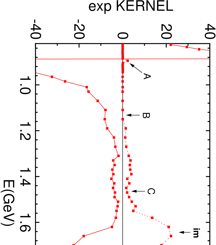
In fig.5 we show the central values for real and imaginary components of the amplitude and, in fig.5, the counterparts for , obtained by using these values into eq.(11). Comparing both figures in the region around , one notes a behaviour similar to a Breit-Wigner function (BWF) for the amplitude and a bare pole for the kernel. This is to be expected, since eq.(8) does indeed transform bare poles into Breit-Wigner functions and, in this process, a resonance in the elastic regime acquires its width, through coupling to and states. The kernel associated with and the corresponding BWF are shown in fig.6. In the case of -waves, the kernel describing the propagation of a single vector resonance is presented in appendix A. In the framework of the system, eq.(23) reads
| (15) |
where is the coupling constant[10]. When a structure of this kind is used into eq.(8), one gets a typical Breit-Wigner amplitude. The width of this resonance is directly proportional to , stressing its dynamic origin.
This pattern is fully backed by field theory. Effective lagrangians, suited to describing low energy mesonic interactions, have been intensively studied in the last three decades[7, 9] and the treatment of resonances has been thoroughly discussed in ref.[10]. Within the lagrangian formalism, the only intrinsic property of a resonance is its mass, which is a real parameter. The width is not intrinsic and has to be generated dynamically, by means of couplings to possible decay products.

The elimination of intermediate states from data yields the kernel , shown in fig.5, where the pole in the real component is clearly visible, at point A. Inspecting the imaginary component, one learns that it vanishes up to point B, indicating the higher end of the elastic regime. From that region onwards, reactions such as or become possible[11]. At higher energies, one finds at least two bumps, associated with resonances. One might also be tempted to interpret data beyond point D as the tail of a third bump. As loops are the only source of imaginary components in hadronic field theory, an imaginary part in is a clear indication of the presence of loops involving heavy intermediate states.
The extraction of information from bumps in the imaginary component requires some theory, since one has to understand how basic dynamics allows several resonances to get dressed. A somewhat detailed discussion of this subject can be found in appendix B. Results given there are consistent with unitarity indicating that, as expected, the imaginary part of cannot be negative. Inspecting the region close to point D in fig.5, one learns that a problem with data may be present there. A comprehensive fit function for , the heavy component of the kernel, is given in eq.(37). However, this function is complicate and we consider two simpler limits, whereby either each resonance develops its own imaginary part independently or this is a fully collective process. The former case corresponds to the direct sum of two Breit-Wigner functions, given by eq.(38), and the latter, to eq.(39), in which bare propagators are added before the unitarization procedure. The distinctive feature of the kernel given by eq.(39) is that it has to vanish at a point at the right of the first peak, as shown in fig.14. This could, in principle, be useful for describing the region around point D in fig.5.
In our instance, the structure of the function has been chosen as a combination of eqs.(38) and (39), which reads
| (16) |
where , , and the are free parameters and
| (17) |
The denominators in eq.(16) are complex and the same happens with the entire function . This choice was motivated by fig.5, since it seems to describe a broad resonance at energies around GeV, associated with , and a dip around GeV, associated with the weighted sum of and .
A possible model for the real background function is given in appendix C. It receives contributions from a contact interaction , associated with chiral symmetry[7], and exchanges of scalar and vector resonances in and channels, denoted by and . Our trial function for the light part of the kernel is written as
| (18) |
where , and are free parameters.
Using the structures given by eqs.(16) and (18), we fitted the phase and modulus for the -wave amplitude with isospin and the results are given in fig.7. We also obtained the couple of functions phase-inelasticity as given in fig.8. The fit information and the values for free parameters can be found in appendix D. In spite of the fact that data may have problems around point D of fig.(5), these results can be considered as being satisfactory.


III summary
We described a procedure which may be instrumental in analyses of low and medium energy hadronic scattering data. The basic idea is that , the kernel of the system, which conveys dynamical information, has a much simpler and transparent structure than the amplitude . In particular, Breit-Wigner trial functions are much more suited to describing the relatively small complex structures associated with possible inelasticities rather than the full interplay between real and imaginary components of the amplitude.
The basic steps of this procedure are summarized below. In the generic process , one departs from the scattering amplitude taken from data and, using the propagator , given by eqs.(6) and (7), into eq.(11), derives a representation for the experimental kernel . This function, in turn, can be decomposed as in eq.(14), which reads
where is real, contains the pole of the lowest resonance, and can be fixed by the neighbourhood of the point at which the phase reaches . The term is complex, conveys information about heavier resonances, and can be represented as a combination of Breit-Wigner functions suited to the case. Finally, is a real contribution which may be either fitted by a polynomial or associated with a model. Once the kernel is known, the full complex structure of the amplitude is recovered by using eq.(8).
ACKNOWLEDGMENTS
The work of P.C.M. was supported by Fundação de Amparo à Pesquisa do Estado de São Paulo (FAPESP).
Appendix A vector amplitude

In the framework of , the -channel tree amplitude , describing the reaction among pseudoscalars , mediated by a vector resonance of mass is given by[10]
| (19) | |||||
where the are structure constants and the are coupling constants. In the center of mass frame, this result can be rewritten in terms of initial and final tree-momenta and as
| (20) | |||||
| (21) | |||||
| (22) |
Projecting out the -wave, one finds the typical structure for the kernel, which is given by
| (23) |
where a factor and the structure constants have been absorbed into the new coupling constants .
In the case , , this result represents the -channel pole of the bare light resonance , shown in Fig.3. Its contribution to the light kernel is
| (24) | |||
| (25) |
where is the coupling constant and is given by eq.(21). The iteration of this kernel, as in Fig.2, gives rise to a geometric series, whose sum is indicated by and reads
| (26) | |||||
| (27) | |||||
| (28) |
where is the dressed resonance propagator. Summing the series (27) and using eq.(25), one may express it as
| (29) |
indicating that the resonance has been dressed. The real part of influences its mass and the imaginary part gives rise to its width.
Appendix B heavy resonances
The amplitude describing the generic elastic reaction is given by the geometric series displayed in Fig.2 and involves both light and heavy kernels, as indicated in Fig.3. The light loop, shown in fig.1, involves just particles and themselves and is described by the function given in eq.(6).
In this Appendix we describe the structure of the heavy kernel , which encompasses all heavy loops, that is, those different from the light one. In order to make our discussion more concrete, we assume that heavy loops represent the propagation of excited states, such as and . This assumption simplifies the presentation, but results do not depend on it and remain valid if other intermediate states are included.
In , the incoming and outgoing light particles and couple to heavy systems, which are assumed to be proper, in the sense that they cannot be split into two parts by cutting intermediate and lines only. These heavy systems contain heavy loops, that give rise to complex components into .
The expression for , in the case of a single heavy resonance , coupled to a single intermediate heavy loop propagator , is a direct generalization of eqs.(26-28) and given by
| (30) | |||||
| (31) | |||||
| (32) |
where is the coupling constant, is the coupling constant of to the heavy loop and the variable is three-momentum inside the heavy loop. In case the resonance can couple to two different intermediate states, labelled by and , eq.(32) becomes
| (33) |
and is illustrated in Fig.10, for and intermediate states.

The inclusion of a second resonance into the problem gives rise to oscillations, due to mixed couplings of the form
| (34) |
The full propagator describing a resonance , which oscillates and still ends up as a resonance , is represented in Fig.11 and corresponds to the series
| (35) | |||||

The propagator for a state , which oscillates and becomes a state , is obtained by multiplying eq.(35) by and reads
| (36) | |||||
The heavy component of the kernel is then given by the diagrams of Fig.12, which correspond to
| (37) |

This result is comprehensive but may be too involved to be used as a practical fit function. We therefore consider two kinds of simplifications, among many other possible. The first one consists in neglecting oscillations between and , by making . This yields and
| (38) |
which represents a simple sum of independent Breit-Wigner functions. Owing to its simplicity, this choice is often made in data analyses and sometimes refered to as isobaric model.
In the second approximation, the coupling between and is kept, but one assumes , and . This gives rise to
| (39) |
The signature of this pattern of composition is that the complex function has to vanish at .
The use of the so called K-matrix approximation yields a complementary useful simplification for . It amounts to assuming that intermediate particles are on-shell and neglecting real parts of heavy propagators. This corresponds to employing
| (40) |
We conclude by discussing the main qualitative features of results presented. In fig.14 we show the behaviour of the single resonance propagator, given by eq.(31), for two different values of the coupling constant . The zero of the real parts occur at , where the imaginary parts reach their maxima. It is worth noting that the imaginary components are not symmetric around this point.


Consequences from the approximation associated with eq.(39) can be seen in the curves of fig.14 where, for the sake of comparison, the case of a single resonance is also shown in curves b. The whole two-resonance propagator vanishes at point P, where the real component crosses the axis and the imaginary component just touches it, since it cannot be negative. This kind of pattern for the imaginary part might, in principle, be related with the behaviour of , at point of fig.5. It is interesting to compare the imaginary parts of curves and around the first peak for, even there, the influence of the second resonance can be seen.
Appendix C background amplitude
We describe below a possible model suited to the case of elastic scattering, inspired in chiral perturbation theory[7, 10]. The regular part of the background kernel, which is real, is assumed to be given by
| (41) |
where is a leading order contact interaction, whereas and are corrections due to - and -channel exchanges of scalar and vector resonances. Using the notation of ref.[10], the -wave components of these contributions are given by
| (42) | |||||
| (43) | |||||
| (44) | |||||
| (46) | |||||
where is the three-momentum in the center of mass, , , and are coupling constants.
Appendix D numerical input
The fit on -wave amplitude with isospin gives for the phase and for the modulus. All values used in this work are expressed bellow.
Masses extracted from PDG 2012[11] in GeV: , , , .
Parameters extracted from scattering data[8]: GeV , .
Fitted parameters with errors in eq.(16): GeV, GeV-2, GeV, GeV-2, GeV , GeV, GeV-2, GeV-2, , GeV, where is related to the heavy mass by
| (48) |
which is an approximation of eq.(22) when one of the masses is considerably greater than the other.
Fitted parameters in eq.(18): , , .
References
- [1] J.A. Oller, Phys. Rev. D71, 054030 (2005); I. Caprini, Phys.Lett. B638, 468 (2006); J. Gasser, B. Kubis and A. Rusetsky Nucl.Phys. B850, 96 (2011); B. Kubis, PoS QNP2012, 027 (2012); B. Kubis, PoS ConfinementX, 240 (2012) ; C. Hanhart, [hep-ph/1311.6627].
- [2] P. C. Magalhães, M. R. Robilotta, K. S. F. F. Guimarães, T. Frederico,W. S. de Paula, I. Bediaga, A. C. dos Reis, and C.M. Maekawa, G.R.S. Zarnauskas, Phys. Rev. D84, 094001 (2011); P. C. Magalhães, M. R. Robilotta, hep-ph/1307.8352; P. C. Magalhães, M. R. Robilotta, hep-ph/1312.2033.
- [3] C.B. Lang, Nucl. Phys. B93, 415 (1975).
- [4] J.A. Oller and E. Oset, Phys. Rev. D 60, 074023 (1999); Nucl. Phys. A 620, 465 (1997); A 652, 407(E) (1999).
- [5] K.P. Khemchandani, A. Martinez Torres, H. Nagahiro and A. Hosaka, Phys.Rev. D88, 114016 (2013);
- [6] J.A. Oller, E. Oset and J.R. Pelaez, Phys.Rev. D59, 074001 (1999), Erratum-ibid. D60, 099906 (1999), Erratum-ibid. D75 (2007) 099903; A. Dobado, J.R. Pelaez, Phys.Rev. D56, 3057 (1997); Phys.Rev. D47, 4883 (1993).
- [7] J. Gasser and H. Leutwyler, Nucl. Phys. B250, 465 (1985); Ann. Phys. 158, 142 (1984).
- [8] D. Aston et al., Nucl.Phys. B 296, 493 (1988).
- [9] S. Weinberg, Physica A 96, 327 (1979).
- [10] G. Ecker, J. Gasser, A. Pich and E. De Rafael, Nucl. Phys. B 321, 311 (1989).
- [11] J.Beringer, Phys.Rev. D86, 010001 (2012).
- [12] M. Jamin, J.A. Oller and A. Pich, Nucl. Phys. B 587, 331 (2000).