Option Pricing Accuracy for Estimated Heston Models

A European call option based on an asset $A$ is a contract signed at time $t=0$, which fixes a strike or exercise price $K$ and a maturity time or exercise date $\tau$. At maturity time, the option holder has the option to buy at price $K$, from the option writer, one share of asset $A$.
Call $X_{t}$ the price of asset $A$ at time $t$. The pay-off of the option at maturity time is then given by $\Psi(X_{\tau})$ where the pay-off function $\Psi(x)$ is defined for $x>0$ by

We systematically assume that the price $X_{t}$ and the squared volatility $Y_{t}$ of $A$ are driven by the joint Heston SDEs (1) (2) with coefficients verifying (3). European call option prices based on asset $A$ verify then a well-known parabolic PDE associated to the elliptic second order differential operator $\mathcal{L}$ defined for $x>0,y>0$ by

The coefficients of $\mathcal{L}$ involve the known risk free rate of return $r$, and the four unknown parameters $\kappa,\theta,\gamma,\rho$ of the Heston SDEs. Note that the drift parameter $\mu$ of these SDEs does not appear in $\mathcal{L}$ .
As in Heston (1993) and Ikonen and Toivanen (2004), the classical coefficient $\lambda\gamma\sqrt{y}$ of $\partial_{y}$ in $\mathcal{L}$ involves the market price of volatility risk $\lambda\geq 0$, which, as in Heston’s classical presentation, is here taken to be a deterministic constant, which theoretically remains the same for all European call options based on the fixed asset $A$ (see Björk (2009)).
The emergence of $\lambda$ in $\mathcal{L}$ and the associated option pricing PDE is due to the fact that the squared volatility $Y_{t}$ is typically a non tradable asset (see Björk (2009) ). Several empirical studies have shown that $\lambda$ cannot be neglected ( Bakshi and Kapadia (2003), Bollerslev et al. (2011), Buraschi and Jackwerth (2001), Carr and Wu (2009), Eraker (2008), Fouque et al. (2000), Lamoureux and Lastrapes (1993)). Since our numerical applications below involve only short term options, we have safely assumed, as in Fouque et al. (2000), that the unknown market price of risk $\lambda$ is a constant which does not depend on time. Since $\lambda$ is unknown, we do estimate $\lambda$ from market data, as outlined in section 7 below.
As is well known (see Heston (1993)), the option price $\mathcal{Z}_{t}$ is of the form

where $g(x,y,t)$ is of class 2 in $(x,y)$ and class 1 in $t$, and is the unique solution of the parabolic PDE

verifying on the boundary $\partial G$ of $G=R^{+}\times R^{+}\times[0,\tau]$ the following boundary conditions

The first condition asserts that at maturity time, the option price is equal to the option pay-off. The second condition states that when the asset price $x=0$, the option price must also be $0$. The third condition is the formal limit, as $y\to 0$, of the PDE (5). Indeed note that, as $y\to 0$, the elliptic operator $\mathcal{L}$ does degenerate into the first order differential operator $D=rx\partial_{x}+\kappa\theta\partial_{y}-r$.
The fourth and fifth boundary conditions require the option price to be approximately linear in the asset price $x$ for large $x$, and to be roughly independent of the squared volatility $y$ for large $y$.
Four of the boundary conditions are standard, namely the initial value (6), the Dirichlet condition (7), and the two Neumann boundary conditions (9) and (10). But the boundary condition (8) at $y=0$ is of a more general type (see Glowinski (2003)).

The coefficients of the elliptic operator $\mathcal{L}$ are explicitly determined by the parameter vector $p=[\kappa,\theta,\gamma,\rho,\lambda]$. Due to the specificity of the 3rd boundary condition in (6) - (10) and to the degenerescence of the elliptic operator $\mathcal{L}$ on the boundary $y=0$, classical generic results on parabolic PDEs (see Singler (2008), Yu et al. (2003)) do not directly imply the differentiability of $g(x,y,t)$ with respect to the vector $p$. To prove differentiability of $g$ with respect to $p$, we now naturally use the Heston closed formulas for $g(x,y,t)$.
The option price $g(x,y,t)$ is actually a function of $x,y,t,p,\tau,K$. For $x,y,t,p,\tau$ fixed, Heston showed that one can write $g(x,y,t)$ as a linear combination of two inverse Fourier transforms

where $F_{1}(z)$ and $F_{2}(z)$ are explicit complex valued functions of $z$ and $x,y,t,p,\tau$ (see Heston (1993)). Heston’s formulas for $F_{1}$ and $F_{2}$ involve sums of complex values rational fractions in $z,x,y,t,p,\tau$ and of square roots of similar complex valued rational fractions.
The option price $g(x,y,t)$ can be computed by numerical implementation of equation (11) because the two integrals in $z>0$ do converge fast enough as $z\to+\infty$. But in this paper, we are specifically focused on quantifying option price sensitivities to estimation errors on the parameter vector $p$, a goal which requires computing the gradient of $g(x,y,t)$with respect to $p$, denoted by

Formally, equation (11) yields the formula

The gradients $\partial_{p}e^{F_{1}(z)}$ and $\partial_{p}e^{F_{2}(z)}$ can be computed explicitly and this yields 10 quite cumbersome formulas for the 5 partial derivatives of $e^{F_{1}(z)}$ and those of $e^{F_{2}(z)}$. Each such formula is a function of $z,x,y,t,p,\tau$ involving compositions of exponentials, square roots, products, and sums of complex valued rational fractions.
We have checked the absolute convergence of the 10 integrals in $z$ involved in equation (13), in particular by verifying that the modulus of their 10 integrands is for large $z>0$ necessarily inferior to $z^{\alpha}e^{-\beta z}$ for some positive $\alpha$ and $\beta$ determined by $x,y,t,p,\tau$. These extensive but tedious verifications have led us in fine to the validation of formula (13).
On the practical level, the full reliability of these formulas is slightly impaired due to the multiple ambiguities generated by simultaneously selecting the determinations of many square roots of complex rational functions (and of their derivatives). Making sure that one chooses the proper combinations of such square roots determinations in all parameter configurations is not a standard computing task, and this point led us to avoid computing $\partial_{p}g$ by numerical implementation of equation (13).
So for concrete numerical computations of the option price gradient $\partial_{p}g$ with respect to the parameter vector $p$, we have definitely preferred to derive and solve the 5 parabolic PDEs (15) verified by the 5 coordinates of $\partial_{p}g$. This generic approach has the merit of extending easily to parameterized pairs of driving SDEs much more general than the Heston SDEs. Moreover the 5 PDE solvers used here are essentially similar and converge reasonably fast as seen below.

In practical option pricing, the parameter vector $p$ has to be estimated from price data, approximate volatility data, and/or observed option trading prices. The unavoidable estimation errors on $p$ necessarily induce option pricing errors.
We define the five sensitivities of the option pricing function $f(x,y,t)=g(x,y,\tau-t)$ with respect to small errors affecting the parameter vector $p$ by the formulas

where all partial derivatives are computed at the point $(x,y,\tau-t)$. These option price sensitivities are hence functions of $(x,y,t,p,\tau,K)$. The numerical computation of option price sensitivities has been explored in Broadie and Kaya (2004); Chan and Joshi (2010) and we propose here an alternate approach.

Differentiating equation (5) with respect to each one of the coordinates of the parameter vector $p$, one obtains the five independent PDEs verified by the 5 coordinates of the gradient $\partial_{p}g(x,y,t)$, in the open domain $0<x,\;0<y,\;0<t<\tau$.

Each one of these five PDEs is associated to five boundary conditions. The first four of these conditions are given in compact form by the following vector equations, where $\mathbf{[0]}$ is the vector of $R^{5}$ with all coordinates equal to 0,

The fifth boundary conditions are obtained by differentiating equation (8) with respect to each one of the parameters. This yields the following boundary conditions, valid for $0<x,\;y=0,\;0<t\leq\tau$,

where $\mathcal{D}$ is the 1st order differential operator given by

We now outline the numerical scheme we have implemented to solve the option price PDE and the five preceding non homogeneous PDEs.

All space partial derivatives in the parabolic PDE (5) have variable coefficients, so that in some parts of the domain the first order derivative terms may dominate the second order terms. To discretize these spatial derivatives we apply a space discretization scheme used in Ikonen and Toivanen (2004) for American options. After discretization, $\mathcal{L}$ becomes a matrix $\mathbf{A}$ well studied in Ikonen and Toivanen (2004).
Recall that M-matrices which are strictly diagonally dominant with positive diagonal elements and non-positive off diagonal elements have good stability properties (see Varga (2000), Windisch (1989)). In general $\mathbf{A}$ is not an M-matrix but as remarked in Ikonen and Toivanen (2004), when the time discretization of (5) has sufficiently small time steps, $\mathbf{A}$ becomes diagonally dominant.
We apply the seven point spatial discretization scheme of Ikonen and Toivanen (2004) to solve for the option price. We use a second order accurate finite difference scheme for the space derivatives, namely the classical central difference scheme for first order derivatives and the usual three point scheme for second order derivatives.
The corresponding finite difference operators are then

On the boundary $j=0$, the derivative in the $y$ direction in (28) is evaluated by the following upwind discretization scheme (see Glowinski (2008)),

As proposed in Ikonen and Toivanen (2004), the mixed derivatives are discretized using a seven point stencil $\delta_{xy}$, where $2\Delta x\;\Delta y\;\delta_{xy}\;g_{i,j}^{k}$ is given by

We handle the Neumann boundary conditions (29) and (30) in the same way as in Ikonen and Toivanen (2004). This space discretization leads to a semi-discrete equation,

where $\mathbf{A}$ is an $mn\times mn$ matrix and $\mathbf{B}$ is a column vector of length $mn$. The vector $\mathbf{g}$ of length $mn$ gathers all the option price values at grid points. The vector $\mathbf{B}$ gathers terms due to the Neumann boundary condition in the $x$ direction and does not depend on $t$.

For time discretization, as in Oosterlee (2003), we use the BDF2 scheme (Backward Difference Formula), which is an implicit scheme with second order accuracy Oosterlee (2003). At time $k\Delta t$ the BDF2 scheme reads,

for $k=1,2,\dots,l-1$. The stability properties of this scheme are studied in Ikonen and Toivanen (2004) and Oosterlee (2003). At each iterate of the BDF2 scheme we require the value of the last two iterates. To obtain the 1st iterate, we use an Implicit Euler scheme Glowinski (2008) : given the initial value $\mathbf{g}^{0}$, we compute $\mathbf{g}^{1}$ by

At moderate grid sizes, we have numerically verified that this choice of space-time discretization of our initial-boundary value problem gives us stable solutions for the option price. At each time step, we use an LU decomposition to solve the following system of linear equations,

where $\mathbf{I}$ is the $mn\times mn$ identity matrix.
Once the function $g$ has been computed on our discrete grid, we solve the sensitivity equations (15)-(19) by a numerical scheme quite similar to the scheme just described. To evaluate the right-hand side of equations (15), we use a central difference scheme to discretize the first spatial derivatives of $g$, a 3-point stencil similar to (32) for the second spatial derivatives of $g$, and a 7 point stencil similar to (33) for the mixed second derivative of $g$. The space-time discretization of the sensitivity equations is the same as above, and we can then solve these discretized equations on the same grid used to compute the option price.
We have verified empirically, by successive grid refinements, that this numerical scheme generates converging approximations for the solutions of the sensitivity equations.

For the stock market example studied below, we fix a subsampling time $T$ and we consider that the $N$ observable data ($U_{n}=X_{nT},\hat{V}_{n}=\hat{Y}_{nT})$ are subsampled from the asset price $X_{t}$ and from estimates $\hat{Y}_{t}$ of the unknown squared volatilities $Y_{t}$. To illustrate how we quantify the impact of parameter estimation errors on option pricing, we study the case of two options written on the index S&P 500. We used a dataset $(SPX)_{n},(VIX)_{n}$ of $N=252$ joint daily observations recorded in 2006 for the S&P 500 index and its approximate annualized volatility VIX. Recall that VIX, as maintained by CBOE, estimates SPX volatility through the implied volatility of options with a 30 day maturity, and is annualized on the standard basis of 252 trading days per year (see Exchange (2003)). We consider the historical time series of $(SPX)_{n}$ and its volatility proxy as being viewed under the market measure $P$. After fixing a conventional time interval $T=1/252$ between two successive daily observations, the daily SPX observations are denoted by $(SPX)_{n}=X_{nT}$ where $(X_{t},Y_{t})$ is an underlying Heston process driven by standard Heston SDEs with unknown parameter vector $\Theta$.
Given N joint daily data $(SPX)_{n},(VIX)_{n}$, we thus set $U_{n}=X_{nT}=(SPX)_{n}$, and we estimate the unobservable squared volatilities $V_{n}=Y_{nT}$ by $\hat{V}_{n}=b\times(VIX)_{n}^{2}$ where the fixed coefficient $b$ simply takes account of the fixed annualization coefficient involved in VIX. As explained in section 5, to estimate $\Theta$, we then first write the explicit formulas (36) giving our consistent maximum likelihood estimators, expressed in terms of the $V_{n}$ and the $U_{n}$; in these formulas, we replace each $V_{n}$ by the observable estimates $\hat{V}_{n}$, and this provides us with observable asymptotically consistent estimators $\hat{\Theta}_{N}$ of $\Theta$.
From the $N=252$ data $(SPX)_{n},(VIX)_{n}$ recorded in 2006, we generate the time series $(SPX)_{n},\hat{V}_{n}=b\times(VIX)_{n}^{2}$ to which we apply our parameter estimators, as defined in equations (35) and (36). This yields the vector $\hat{\Theta}$ of estimated parameter values

The estimated drift $\mu$ is not listed since it has no impact on option pricing.
As outlined in section 5, we then fix $\Theta$ at the estimated values just obtained to simulate 5000 trajectories of the just fitted Heston SDEs, and this enables the computation of empirical evaluations for the root mean squared errors of estimation $s_{\kappa},s_{\theta},s_{\gamma},s_{\rho}$. This easily yields the values

The number $N=252$ of joint daily observations is realistic but rather small, so that the relative errors of estimation on SDEs parameters are naturally still fairly high.
For numerical evaluations below, we consider that with reasonably high probability, the parameters $\kappa,\;\theta,\;\gamma,\;\rho$ belong to four intervals centered around $\hat{\kappa},\;\hat{\theta},\;\hat{\gamma},\;\hat{\rho}$, and with half-widths $\hat{s}_{\kappa},\;\hat{s}_{\theta},\;\hat{s}_{\gamma},\;\hat{s}_{\rho}$. The product $J\subset R^{4}$ of these four intervals is then a high probability “localization box” for the true vector $\Theta$ of unknown parameters.

To compute the option price, one first has to estimate the unknown market price $\lambda$ of volatility risk which depends on investors preferences, liquidity concerns, risk aversion, etc. For various approaches to estimate $\lambda$, see for instance Björk (2009), Fouque et al. (2000), Heston (1993), Lamoureux and Lastrapes (1993).
In the spirit of Fouque et al. (2000), and since in our numerical examples we consider only short term options maturing within the same short period of time, we have safely assumed that $\lambda$ is an unknown constant, and we use a small pool of short term options to estimate $\lambda$ as follows.
Consider $q$ benchmark options $\Omega_{j}$, $j=1\ldots q$, with strikes $K_{j}$ and maturity $\tau_{j}$, written on the same underlying asset. Consider the underlying asset denoted by $X_{t}$ and its volatility $Y_{t}$ are driven by SDEs (1)-(2). Call $T$ the user selected time step between observations. Then for each day $k$, let $X_{kT}$ be the closing asset price and $\Omega_{j}(kT)$ be the average of closing bid and ask for $\Omega_{j}$. We will estimate the unknown constant $\lambda$ by minimizing a distance between the predicted option price and the observed market option price across all times $t$ and all options $\Omega_{j}$. Let $f_{j,\lambda}(x,y,t)$ be the solution of the option pricing PDE (5) for option $\Omega_{j}$. The predicted option price $\hat{\Omega}_{j}(kT)$ for day $k$ becomes $f_{j,\lambda}(X_{kT},Y_{kT},kT)$. To compare this option price predictor to the observed option price $\Omega_{j}(kT)$, we compute the root mean squared prediction error $RMS_{j}(\lambda)$ defined by

Let $p_{j}$ be the median price of $\Omega_{j}$ over its lifetime. To combine option pricing accuracy across multiple options, introduce the relative size of pricing prediction errors $RMS_{j}(\lambda)/p_{j}$ for each $j$. Consider any estimator $\hat{\lambda}$ of $\lambda$, computed from the pool of options $\Omega_{j}$. If $\hat{\lambda}$ takes the value $L$, we quantify the associated prediction error $\text{prederr}\,(L)$ by the median of relative pricing prediction errors over all benchmark options, so that

We will hence compute our estimator $\hat{\lambda}$ by minimizing the median pricing error $\text{prederr}\,(L)$ overall $L$, so that $\hat{\lambda}=L*$ where $L*>0$ is determined by

Note that our approach to estimate $\lambda$ works just as well if we replace the median by the mean of the $RMS_{j}/p_{j}$; but we prefer to use the median to gain in robustness to outliers.

For the option pricing sensitivity results presented below, we have focused on the S&P 500 index SPX and its approximate annualized volatility VIX in the first quarter of 2007. In the previous section, we have modeled the joint process $(SPX,VIX)$ by joint Heston SDEs with sub-sampling time $T=1/252$ and parameters estimated on the basis of 252 daily observations recorded in 2006.
To estimate $\lambda$ we have selected 16 benchmark options $\Omega_{j}$ observed over 22 trading days. Eight of these options were maturing on Feb 17th 2007, with strike prices 1380, 1400, 1410, 1420, 1425, 1430, 1450, 1460. The other 8 options had the same strike prices but with maturity date Mar 17th 2007.
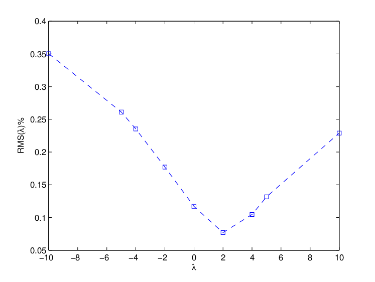
The risk free rate of return is set at $r=1\%$. Fix any tentative value $L$ of the unknown $\lambda$ As indicated above, for each option $\Omega_{j}$, we solve the $\Omega_{j}$ pricing PDE to evaluate the mean squared difference $RMS_{j}(L)$ between real and computed $\Omega_{j}$ price over the 22 days option lifetime. We then compute the median $\text{prederr}\,(L)$ of the 16 relative pricing errors $RMS_{j}(L)/p_{j}$ where $p_{j}$ is the median price of $\Omega_{j}$ over its lifetime. The graph of $\text{prederr}\,(L)$ is displayed in figure 1 as a function of $L$, which reaches a minimum of $8\%$ for $L*=2.0$. We thus estimate the unknown $\lambda$ by $\hat{\lambda}=L*=2.0$ This estimate of $\lambda$ then enables us to compute all the of option pricing sensitivities we present for options based on S&P 500.

References

- Achdou and Pironneau (2005) Achdou, Y. and Pironneau, O., Computational methods for option pricing, 2005, Society for Industrial Mathematics.
- Ait-Sahalia and Kimmel (2007) Ait-Sahalia, Y. and Kimmel, R., Maximum likelihood estimation of stochastic volatility models. Journal of Financial Economics, 2007, 83, 413–452.
- Andersen et al. (2003) Andersen, T.G., Bollerslev, T., Diebold, F.X. and Labys, P., Modeling and forecasting realized volatility. Econometrica, 2003, 71, 579–625.
- Andersen et al. (2009) Andersen, T.G., Davis, R.A., Kreiß, J.P. and Mikosch, T.V., Handbook of Financial Time Series, 2009, Springer.
- Atiya and Wall (2009) Atiya, A.F. and Wall, S., An analytic approximation of the likelihood function for the Heston model volatility estimation problem. Quantitative Finance, 2009, 9, 289–296.
- Avellaneda et al. (2003) Avellaneda, M., Boyer-Olson, D., Friz, P. et al., Application of large deviation methods to the pricing of index options in finance. Comptes Rendus Mathematique, 2003, 336, 263–266.
- Azencott et al. (2015a) Azencott, R., Beri, A., Ren, P. and Timofeyev, I., Parametric estimation of the volatility equation in the Heston Model using indirect observations. , 2015a Pre print.
- Azencott et al. (2015b) Azencott, R., Ren, P. and Timofeyev, I., Parametric Estimation from Approximate Data: Non-Gaussian Diffusions. arXiv:1501.05370v1 [math.PR], 2015b.
- Azencott and Gadhyan (2009) Azencott, R. and Gadhyan, Y., Accurate parameter estimation for coupled stochastic dynamics. In Proceedings of the Dynamical Systems and Differential Equations. Proceedings of the 7th AIMS international conference, Arlington, Texas, DCDS Supplement, pp. 44–53, 2009.
- Azencott and Gadhyan (2015) Azencott, R. and Gadhyan, Y., Accuracy of Maximum Likelihood Parameter Estimators for Heston volatility SDEs. Journal of Statistical Physics, 2015, 159, 393–420.
- Bakshi et al. (1997) Bakshi, G., Cao, C. and Chen, Z., Empirical performance of alternative option pricing models. Journal of Finance, 1997, 52, 2003–2049.
- Bakshi and Kapadia (2003) Bakshi, G. and Kapadia, N., Delta-hedged gains and the negative market volatility risk premium. Review of Financial Studies, 2003, 16, 527–566.
- Barndorff-Nielsen (2002) Barndorff-Nielsen, O.E., Econometric analysis of realized volatility and its use in estimating stochastic volatility models. Journal of the Royal Statistical Society: Series B (Statistical Methodology), 2002, 64, 253–280.
- Bates (1996) Bates, D.S., Jumps and stochastic volatility: Exchange rate processes implicit in Deutsche Mark options. Review of financial studies, 1996, 9, 69–107.
- Björk (2009) Björk, T., Arbitrage theory in continuous time, 2009, Oxford Univ Press.
- Black and Scholes (1973) Black, F. and Scholes, M., The pricing of options and corporate liabilities. Journal of Political Economy, 1973, 81.
- Black (1976) Black, F., Studies of Stock Price Volatility Changes. , 1976.
- Bollerslev et al. (2011) Bollerslev, T., Gibson, M. and Zhou, H., Dynamic estimation of volatility risk premia and investor risk aversion from option-implied and realized volatilities. Journal of Econometrics, 2011, 160, 235–245.
- Bollerslev and Zhou (2002) Bollerslev, T. and Zhou, H., Estimating stochastic volatility diffusion using conditional moments of integrated volatility. Journal of Econometrics, 2002, 109, 33–65.
- Broadie and Kaya (2004) Broadie, M. and Kaya, O., Exact simulation of option greeks under stochastic volatility and jump diffusion models. In Proceedings of the Simulation Conference, 2004. Proceedings of the 2004 Winter, Vol. 2, pp. 1607–1615, 2004.
- Broto and Ruiz (2004) Broto, C. and Ruiz, E., Estimation methods for stochastic volatility models: a survey. Journal of Economic Surveys, 2004, 18, 613–649.
- Buraschi and Jackwerth (2001) Buraschi, A. and Jackwerth, J., The price of a smile: Hedging and spanning in option markets. Review of Financial Studies, 2001, 14, 495–527.
- Carr and Madan (1999) Carr, P. and Madan, D., Option pricing and the fast Fourier transform. Journal of Computational Finance, 1999, 2, 61–73.
- Carr and Wu (2009) Carr, P. and Wu, L., Variance risk premiums. Review of Financial Studies, 2009, 22, 1311–1341.
- Chan and Joshi (2010) Chan, J.H. and Joshi, M., First and second order greeks in the Heston model. Available at SSRN 1718102, 2010.
- Chernov and Ghysels (2000) Chernov, M. and Ghysels, E., A study towards a unified approach to the joint estimation of objective and risk neutral measures for the purpose of options valuation. Journal of Financial Economics, 2000, 56, 407–458.
- Comte et al. (1998) Comte, F., Renault, E. et al., Long memory in continuous-time stochastic volatility models. Mathematical Finance, 1998, 8, 291–323.
- Cox et al. (1985) Cox, J., Ingersoll Jr, J. and Ross, S., A theory of the term structure of interest rates. Econometrica: Journal of the Econometric Society, 1985, 53, 385–407.
- Dacunha-Castelle and Florens-Zmirou (1986) Dacunha-Castelle, D. and Florens-Zmirou, D., Estimation of the coefficients of a diffusion from discrete observations. Stochastics An International Journal of Probability and Stochastic Processes, 1986, 19, 263–284.
- Duffie et al. (2000) Duffie, D., Pan, J. and Singleton, K., Transform analysis and asset pricing for affine jump-diffusions. Econometrica, 2000, 68, 1343–1376.
- Eraker (2008) Eraker, B., The Volatility Premium. , 2008.
- Exchange (2003) Exchange, C.B.O., VIX White Paper. URL: http://www. cboe. com/micro/vix/vixwhite. pdf, 2003.
- Feller (1951) Feller, W., Two singular diffusion problems. Annals of Mathematics, 1951, 54, 173–182.
- Fouque et al. (2000) Fouque, J.P., Papanicolaou, G. and Sircar, K.R., Mean-reverting stochastic volatility. International Journal of Theoretical and Applied Finance, 2000, 3, 101–142.
- Gadhyan (2010) Gadhyan, Y., Option Pricing Accuracy for Estimated Stochastic Volatility Models. PhD thesis, University of Houston, 2010.
- Gallant and Tauchen (1996) Gallant, A.R. and Tauchen, G., Which moments to match?. Econometric Theory, 1996, 12, 657–681.
- Garman and Klass (1980) Garman, M.B. and Klass, M.J., On the estimation of security price volatilities from historical data. Journal of business, 1980, pp. 67–78.
- Gatheral et al. (2014) Gatheral, J., Jaisson, T. and Rosenbaum, M., Volatility is rough. Available at SSRN 2509457, 2014.
- Genon-Catalot and Jacod (1994) Genon-Catalot, V. and Jacod, J., Estimation of the diffusion coefficient for diffusion processes: random sampling. Scandinavian Journal of Statistics, 1994, 21, 193–221.
- Genon-Catalot et al. (1999) Genon-Catalot, V., Jeantheau, T. and Laredo, C., Parameter estimation for discretely observed stochastic volatility models. Bernoulli, 1999, 5, 855–872.
- Glowinski (2003) Glowinski, R., Handbook of numerical analysis, 2003, North-Holland Amsterdam.
- Glowinski (2008) Glowinski, R., Numerical methods for nonlinear variational problems, 2008, Springer-Verlag.
- Haentjens (2013) Haentjens, T., Efficient and stable numerical solution of the Heston–Cox–Ingersoll–Ross partial differential equation by alternating direction implicit finite difference schemes. International Journal of Computer Mathematics, 2013, 90, 2409–2430.
- Heston (1993) Heston, S., A closed-form solution for options with stochastic volatility with applications to bond and currency options. Review of Financial Studies, 1993, 6, 327–343.
- Hull and White (1987) Hull, J. and White, A., The pricing of options on assets with stochastic volatilities. Journal of Finance, 1987, 42, 281–300.
- Ikonen and Toivanen (2004) Ikonen, S. and Toivanen, J., Operator splitting methods for American option pricing. Applied Mathematics Letters, 2004, 17, 809–814.
- Jacquier et al. (2002) Jacquier, E., Polson, N.G. and Rossi, P.E., Bayesian analysis of stochastic volatility models. Journal of Business & Economic Statistics, 2002, 20, 69–87.
- Johnson and Shanno (1987) Johnson, H. and Shanno, D., Option Pricing when the Variance Is Changing. Journal of Financial and Quantitative Analysis, 1987, 22, 143–151.
- Kim et al. (1998) Kim, S., Shephard, N. and Chib, S., Stochastic volatility: likelihood inference and comparison with ARCH models. The Review of Economic Studies, 1998, 65, 361–393.
- Lamoureux and Lastrapes (1993) Lamoureux, C.G. and Lastrapes, W.D., Forecasting stock-return variance: Toward an understanding of stochastic implied volatilities. Review of Financial Studies, 1993, 6, 293–326.
- Melino and Turnbull (1990) Melino, A. and Turnbull, S., Pricing foreign currency options with stochastic volatility. Journal of Econometrics, 1990, 45, 239–265.
- Oosterlee (2003) Oosterlee, C., On multigrid for linear complementarity problems with application to American-style options. Electronic Transactions on Numerical Analysis, 2003, 15, 165–185.
- O’sullivan and O’sullivan (2013) O’sullivan, C. and O’sullivan, S., PRICING EUROPEAN AND AMERICAN OPTIONS IN THE HESTON MODEL WITH ACCELERATED EXPLICIT FINITE DIFFERENCING METHODS. International Journal of Theoretical and Applied Finance (IJTAF), 2013, 16.
- Pan (2002) Pan, J., The jump-risk premia implicit in options: Evidence from an integrated time-series study. Journal of financial economics, 2002, 63, 3–50.
- Ren (2014) Ren, P., Parametric Estimation of the Heston model under the Indirect Observability Framework [online]. , 2014. (accessed ????).
- Scott (1987) Scott, L.O., Option Pricing when the Variance Changes Randomly: Theory, Estimation, and an Application. Journal of Financial and Quantitative Analysis, 1987, 22, 419–438.
- Shephard (2005) Shephard, N., Stochastic Volatility.. Economics Group, Nuffield College, University of Oxford, Economics Papers, 2005.
- Singler (2008) Singler, J., Differentiability with respect to parameters of weak solutions of linear parabolic equations. Mathematical and Computer Modelling, 2008, 47, 422–430.
- Stein and Stein (1991) Stein, E. and Stein, J., Stock price distributions with stochastic volatility: an analytic approach. Review of Financial Studies, 1991, 4, 727–752.
- Stein (1989) Stein, J., Overreactions in the options market. The Journal of Finance, 1989, 44, 1011–1023.
- Varga (2000) Varga, R., Matrix Iterative Analysis, 2000, Springer, Berlin.
- Wiggins (1987) Wiggins, J., Option values under stochastic volatility: Theory and empirical estimates. Journal of Financial Economics, 1987, 19, 351–372.
- Windisch (1989) Windisch, G., M-matrices in numerical analysis, Vol. 115, , 1989, Teubner.
- Yu et al. (2003) Yu, W., Zhang, F. and Xie, W., Differentiability of C0-semigroups with respect to parameters and its application. Journal of Mathematical Analysis and Applications, 2003, 279, 78–96.