⁵⁵footnotetext: Upon publication, we will make replication materials available through a public archive. Many of the methods described in this paper can be implemented using our accompanying open-source R package, which is available on CRAN.

Generalizing the Network Scale-Up Method:
A New Estimator for the Size of Hidden Populations¹¹ 1 The authors thank Alexandre Abdo, Francisco Bastos, Russ Bernard, Neilane Bertoni, Dimitri Fazito, Sharad Goel, Wolfgang Hladik, Jake Hofman, Mike Hout, Karen Levy, Rob Lyerla, Mary Mahy, Chris McCarty, Maeve Mello, Tyler McCormick, Damon Phillips, Justin Rao, Adam Slez, and Tian Zheng for helpful discussions. This research was supported by The Joint United Nations Programme on HIV/AIDS (UNAIDS), NSF (CNS-0905086), and NIH/NICHD (R01-HD062366, R01-HD075666, & R24-HD047879). Some of this research was conducted while MJS was an employee Microsoft Research. The opinions expressed here represent the views of the authors and not the funding agencies. ⁴⁴ 4 Department of Sociology, Princeton University, Princeton, NJ, USA ⁶⁶ 6 Word count: main text 6,520 words; abstract 164 words

Dennis M. Feehan²² 2 Department of Demography, University of California, Berkeley, CA, USA and Matthew J. Salganik³³ 3 Office of Population Research, Princeton University, Princeton, NJ, USA ⁴⁴footnotemark: 4

August 24, 2026

Abstract

The network scale-up method enables researchers to estimate the size of hidden populations, such as drug injectors and sex workers, using sampled social network data. The basic scale-up estimator offers advantages over other size estimation techniques, but it depends on problematic modeling assumptions. We propose a new generalized scale-up estimator that can be used in settings with non-random social mixing and imperfect awareness about membership in the hidden population. Further, the new estimator can be used when data are collected via complex sample designs and from incomplete sampling frames. However, the generalized scale-up estimator also requires data from two samples: one from the frame population and one from the hidden population. In some situations these data from the hidden population can be collected by adding a small number of questions to already planned studies. For other situations, we develop interpretable adjustment factors that can be applied to the basic scale-up estimator. We conclude with practical recommendations for the design and analysis of future studies.

1 Introduction

Many important problems in social science, public health, and public policy require estimates of the size of hidden populations. For example, in HIV/AIDS research, estimates of the size of the most at-risk populations—drug injectors, female sex workers, and men who have sex with men—are critical for understanding and controlling the spread of the epidemic. However, researchers and policy makers are unsatisfied with the ability of current statistical methods to provide these estimates (Joint United Nations Programme on HIV/AIDS,, 2010). We address this problem by improving the network scale-up method, a promising approach to size estimation. Our results are immediately applicable in many substantive domains in which size estimation is challenging, and the framework we develop advances the understanding of sampling in networks more generally.

The core insight behind the network scale-up method is that ordinary people have embedded within their personal networks information that can be used to estimate the size of hidden populations, if that information can be properly collected, aggregated, and adjusted (Bernard et al.,, 1989; Bernard et al.,, 2010). In a typical scale-up survey, randomly sampled adults are asked about the number of connections they have to people in a hidden population (e.g., “How many people do you know who inject drugs?”) and a series of similar questions about groups of known size (e.g., “How many widowers do you know?”; “How many doctors do you know?”). Responses to these questions are called aggregate relational data (McCormick et al.,, 2012).

To produce size estimates from aggregate relational data, previous researchers have begun with the basic scale-up model, which makes three important assumptions: (i) social ties are formed completely at random (i.e., random mixing), (ii) respondents are perfectly aware of the characteristics of their alters, and (iii) respondents are able to provide accurate answers to survey questions about their personal networks. From the basic scale-up model Killworth et al., 1998b () derived the basic scale-up estimator. This estimator, which is widely used in practice, has two main components. For the first component, the aggregate relational data about the hidden population are used to estimate the number of connections that respondents have to the hidden population. For the second component, the aggregate relational data about the groups of known size are used to estimate the number of connections that respondents have in total. For example, a researcher might estimate that members of her sample have 5,000 connections to people who inject drugs and 100,000 connections in total. The basic scale-up estimator combines these pieces of information to estimate that 5% ( $5,000/100,000$ ) of the population injects drugs. This estimate is a sample proportion, but rather than being taken over the respondents, as would be typical in survey research, the proportion is taken over the respondents’ alters. Researchers who desire absolute size estimates multiply the alter sample proportion by the size of the entire population, which is assumed to be known (or estimated using some other method).

Unfortunately, the three assumptions underlying the basic scale-up model have all been shown to be problematic. Scale-up researchers call violations of the random mixing assumption barrier effects (Killworth et al.,, 2006; Zheng et al.,, 2006; Maltiel et al.,, 2015); they call violations of the perfect awareness assumption transmission error (Shelley et al.,, 1995; Shelley et al.,, 2006; Killworth et al.,, 2006; Salganik et al., 2011b, ; Maltiel et al.,, 2015); and they call violations of the respondent accuracy assumption recall error (Killworth et al.,, 2003; Killworth et al.,, 2006; McCormick and Zheng,, 2007; Maltiel et al.,, 2015).

Hidden population(s)	Location	Citation
Mortality in earthquake	Mexico City, Mexico	(Bernard et al.,, 1989)
Rape victims	Mexico City, Mexico	(Bernard et al.,, 1991)
HIV prevalence, rape, and homelessness	U.S.	(Killworth et al., 1998b, )
Heroin use	14 U.S. cities	(Kadushin et al.,, 2006)
Choking incidents in children	Italy	(Snidero et al.,, 2007; Snidero et al.,, 2009; Snidero et al.,, 2012)
Groups most at-risk for HIV/AIDS	Ukraine	(Paniotto et al.,, 2009)
Heavy drug users	Curitiba, Brazil	(Salganik et al., 2011a, )
Groups most at-risk for HIV/AIDS	Kerman, Iran	(Shokoohi et al.,, 2012)
Men who have sex with men	Japan	(Ezoe et al.,, 2012)
Groups most at-risk for HIV/AIDS	Almaty, Kazakhstan	(Scutelniciuc, 2012a, )
Groups most at-risk for HIV/AIDS	Moldova	(Scutelniciuc, 2012b, )
Groups most at-risk for HIV/AIDS	Thailand	(Aramrattan and Kanato, 8, 30)
Groups most at-risk for HIV/AIDS	Rwanda	(Rwanda Biomedical Center,, 2012)
Groups most at-risk for HIV/AIDS	Chongqing, China	(Guo et al.,, 2013)
Groups most at-risk for HIV/AIDS	Tabriz, Iran	(Khounigh et al.,, 2014)
Men who have sex with men	Taiyuan, China	(Jing et al.,, 2014)
Drug and alcohol users	Kerman, Iran	(Sheikhzadeh et al.,, 2014)
Men who have sex with men	Shanghai, China	(Wang et al.,, 2015)

Table 1: Network scale-up studies that have been completed.

In this paper, we develop a new approach to producing size estimates from aggregate relational data. Rather than depending on the basic scale-up model or its variants (e.g., Maltiel et al., (2015)), we use a simple identity to derive a series of new estimators. Our new approach reveals that one of the two main components of the basic scale-up estimator is problematic. Therefore, we propose a new estimator—the generalized scale-up estimator—that combines the aggregate relational data traditionally used in scale-up studies with similar data collected from the hidden population. Collecting data from the hidden population is a major departure from current scale-up practice, but we believe that it enables a more principled approach to estimation. For researchers who are not able to collect data from the hidden population, we propose a series of adjustment factors that highlight the possible biases of the basic scale-up estimator. Ultimately, researchers must balance the trade-offs between the basic scale-up estimator, generalized scale-up estimator, and other size estimation techniques based on the specific features of their research setting.

In the next section, we derive the generalized scale-up estimator, and we describe the data collection procedures needed to use it. In Section 3, we compare the generalized and basic scale-up approaches analytically and with simulations; our comparison leads us to propose a decomposition that separates the difference between the two approaches into three measurable and substantively meaningful factors (Equation 15). In Section 4 we make practical recommendations for the design and analysis of future scale-up studies, and in Section 5, we conclude with an discussion of next steps. Online Appendices A - G provide technical details and supporting arguments.

2 The generalized scale-up estimator

The generalized scale-up estimator can be derived from a simple accounting identity that requires no assumptions about the underlying social network structure in the population. Figure 1 helps illustrate the derivation, which was inspired by earlier research on multiplicity estimation (Sirken,, 1970) and indirect sampling (Lavallée,, 2007). Consider a population of 7 people, 2 of whom are drug injectors (Figure 1). In this population, two people are connected by a directed edge $i\rightarrow j$ if person $i$ would count person $j$ as a drug injector when answering the question “How many drug injectors do you know?” Whenever $i\rightarrow j$ , we say that $i$ makes an out-report about $j$ and that $j$ receives an in-report from $i$ .¹¹ 1 Throughout the paper, we only consider the case where $i$ never reports $j$ more than once.

Each person can be viewed as both a source of out-reports and a recipient of in-reports, and in order to emphasize this point, Figure 1 shows the population with each person represented twice: on the left as a sender of out-reports and on the right as a receiver of in-reports. This visual representation highlights the following identity:

\displaystyle\text{total out-reports}=\text{total in-reports}.

(1)

Despite its simplicity, the identity in Equation 1 turns out to be very useful because it leads directly to the new estimator that we propose.

Figure 1: Illustration of the derivation of the generalized scale-up estimator. Panel (a) shows a population of 7 people, 2 of whom are drug injectors (shown in grey). A directed edge

i\rightarrow j

indicates that

i

counts

j

as a drug injector when answering the question “How many drug injectors do you know?” Panel (b) shows the same population, but redrawn so that each person now appears twice: as a source of out-reports, on the left, and as a recipient of in-reports, on the right. This arrangement shows that total out-reports and total in-reports must be equal. Panel (c) shows the same population again, but now some of the people are in the frame population

F

and some are not. In real scale-up studies, we can only learn about out-reports from the frame population.

In order to derive an estimator from Equation 1, we must define some notation. Let $U$ be the entire population, and let $H\subset U$ be the hidden population. Further, let $y_{i,H}$ be the total number of out-reports from person $i$ (i.e., person $i$ ’s answer to the question “How many drug injectors do you know?”). For example, Figure 1 shows that person 5 would report knowing 1 drug injector, so $y_{5,H}=1$ . Let $v_{i,U}$ be the total number of in-reports to $i$ if everyone in $U$ is interviewed; that is, $v_{i,U}$ is the visibility of person $i$ to people in $U$ . For example, Figure 1 shows person 5 would be reported as a drug injector by 3 people so $v_{5,U}=3$ . Since total out-reports must equal total in-reports, it must be the case that

\displaystyle y_{U,H}=v_{U,U},

(2)

where $y_{U,H}=\sum_{i\in U}y_{i,H}$ and $v_{U,U}=\sum_{i\in U}v_{i,U}$ . Multiplying both sides of Equation 2 by $N_{H}$ , the number of people in the hidden population, and then rearranging terms, we get

\displaystyle N_{H}=\frac{y_{U,H}}{v_{U,U}/N_{H}}.

(3)

Equation 3 is an expression for the size of the hidden population that does not depend on any assumptions about network structure or reporting accuracy; it is just a different way of expressing the identity that the total number of out-reports must equal the total number of in-reports. If we could estimate the two terms on the right side of Equation 3—one term related to out-reports ( $y_{U,H}$ ) and one term related to in-reports ( $v_{U,U}/N_{H}$ )—then we could estimate $N_{H}$ .

However, in order to make the identity in Equation 3 useful in practice we need to modify it to account for an important logistical requirement of survey research. In real scale-up studies, researchers do not sample from the entire population $U$ , but instead they sample from a subset of $U$ called the frame population, $F$ . For example, in almost all scale-up studies the frame population has been adults (but note that our mathematical results hold for any frame population). In standard survey research, restricting interviews to a frame population does not cause problems because inference is being made about the frame population. In other words, when respondents report about themselves it is clear to which group inferences apply. However, with the scale-up method, respondents report about others, so the group that inferences are being made about is not necessarily the same as the group that is being interviewed. As we show in Section 4.2, failure to consider this fact requires the introduction of an awkward adjustment factor that had previously gone unnoticed. Here, we avoid this awkward adjustment factor by deriving an identity explicitly in terms of the frame population. Restricting our attention to out-reports coming from people in the frame population, it must be the case that

N_{H}=\frac{y_{F,H}}{v_{U,F}/N_{H}},

(4)

where $y_{F,H}=\sum_{i\in F}y_{i,H}$ and $v_{U,F}=\sum_{i\in U}v_{i,F}$ . The only difference between Equation 3 and Equation 4 is that Equation 4 restricts out-reports and in-reports to come from people in the frame population (Figure 1). The identity in Equation 4 is extremely general: it does not depend on any assumptions about the relationship between the entire population $U$ , the frame population $F$ , and the hidden population $H$ . For example, it holds if no members of the hidden population are in the frame population, if there are barrier effects, and if there are transmission errors. Thus, if we could estimate the two terms on the right side of Equation 4—one term related to out-reports ( $y_{F,H}$ ) and one term related to in-reports ( $v_{U,F}/N_{H}$ )—then we could estimate $N_{H}$ under very general conditions.

Unfortunately, despite repeated attempts, we were unable to develop a practical method for estimating the term related to in-reports ( $v_{U,F}/N_{H}$ ). However, if we make an assumption about respondents’ reporting behavior, then we can re-express Equation 4 as an identity made up of quantities that we can actually estimate. Specifically, if we assume that the out-reports from people in the frame population only include people in the hidden population, then it must be the case that the visibility of everyone not in the hidden population is 0: $v_{i,F}=0\mbox{ for all }i\notin H$ . In this case, we can re-write Equation 4 as

\displaystyle N_{H}=\frac{y_{F,H}}{v_{H,F}/N_{H}}=\frac{y_{F,H}}{\bar{v}_{H,F}}\quad\mbox{if }v_{i,F}=0\mbox{ for all }i\notin H,

(5)

where $\bar{v}_{H,F}=v_{H,F}/N_{H}$ .

To understand the reporting assumption substantively, consider the two possible types of reporting errors: false positives and false negatives. Previous scale-up research on transmission error focused on the problem of false negatives, where a respondent is connected to a member of the hidden population but does not report this, possibly because she is not aware that the person she is connected to is in the hidden population (Bernard et al.,, 2010). Since hidden populations like drug injectors are often stigmatized, it is reasonable to suspect that false negatives will be a serious problem for the scale-up method. Fortunately, Equation 5 holds even if there are false negative reporting errors. However, false positives—which do not seem to have been considered previously in the scale-up literature—are also possible. For example, a respondent who is not connected to any drug injectors might report that one of her acquaintances is a drug injector. These false positive reports are not accounted for in the identity in Equation 5 and the estimators that we derive subsequently. If false positive reports exist, they will introduce a positive bias into estimates from the generalized scale-up estimator. Therefore, in Online Appendix A we (i) formally define an interpretable measure of false positive reports, the precision of out-reports; (ii) analytically show the bias in size estimates as a function of the precisions of out-reports; and (iii) discuss two research designs that could enable researchers to estimate the precision of out-reports.

2.1 Estimating $N_{H}$ from sampled data

Equation 5 relates our quantity of interest, the size of the hidden population ( $N_{H}$ ), to two other quantities: the total number of out-reports from the frame population ( $y_{F,H}$ ) and the average number of in-reports in the hidden population ( $\bar{v}_{H,F}$ ). We now show how to estimate $y_{F,H}$ with a probability sample from the frame population and $\bar{v}_{H,F}$ with a relative probability sample from the hidden population.

The total number of out-reports ( $y_{F,H}$ ) can be estimated from respondents’ reported number of connections to the hidden population,

\displaystyle\widehat{y}_{F,H}=\sum_{i\in s_{F}}\frac{y_{i,H}}{\pi_{i}},

(6)

where $s_{F}$ denotes the sample, $y_{i,H}$ denotes the reported number of connections between $i$ and $H$ , and $\pi_{i}$ is $i$ ’s probability of inclusion from a conventional probability sampling design from the frame population. Because $\widehat{y}_{F,H}$ is a standard Horvitz-Thompson estimator, it is consistent and unbiased as long as all members of $F$ have a positive probability of inclusion under the sampling design (Sarndal et al.,, 1992); for a more formal statement, see Result B.2. This estimator depends only on an assumption about the sampling design for the frame population, and in Table D.2 we show the sensitivity of our estimator to violations of this assumption.

Estimating the average number of in-reports for the hidden population ( $\bar{v}_{H,F}$ ) is more complicated. First, it will usually be impossible to obtain a conventional probability sample from the hidden population. As we show below, however, estimating $\bar{v}_{H,F}$ only requires a relative probability sampling design in which hidden population members have a nonzero probability of inclusion and respondents’ probabilities of inclusion are known up to a constant of proportionality, $c\pi_{i}$ (see Online Appendix C.1 for a more precise definition). Of course, even selecting a relative probability sample from a hidden population can be difficult.

A second problem arises because we do not expect respondents to be able to easily and accurately answer direct questions about their visibility ( $v_{i,F}$ ). That is, we do not expect respondents to be able to answer questions such as “How many people on the sampling frame would include you when reporting a count of the number of drug injectors that they know?” Instead, we propose asking hidden population members a series of questions about their connections to certain groups and their visibility to those groups. For example, each sampled hidden population respondent could be asked “How many widowers do you know?” and then “How many of these widowers are aware that you inject drugs?” This question pattern can be repeated for many groups (e.g., widowers, doctors, etc.). We call data with this structure enriched aggregate relational data to emphasize its similarity to the aggregate relational data that is familiar to scale-up researchers. An interviewing procedure called the game of contacts enables researchers to collect enriched aggregated relational data, even in realistic field settings (Salganik et al., 2011b, ; Maghsoudi et al.,, 2014).

Given a relative probability sampling design and enriched aggregate relational data, we can now formalize our proposed estimator for $\bar{v}_{H,F}$ . Let $A_{1},A_{2},\ldots,A_{J}$ , be the set of groups about which we collect enriched aggregate relational data (e.g., widowers, doctors, etc). Here, to keep the notation simple, we assume that these groups are all contained in the frame population, so that $A_{j}\subset F$ for all $j$ ; in Online Appendix C.4 we extend the results to groups that do not meet this criterion. Let $\mathcal{A}$ be the concatenation of these groups, which we call the probe alters. For example, if $A_{1}$ is widowers and $A_{2}$ is doctors, then the probe alters $\mathcal{A}$ is the collection of all widowers and all doctors, with doctors who are widowers included twice. Also, let $\tilde{v}_{i,A_{j}}$ be respondent $i$ ’s report about her visibility to people in $A_{j}$ and let $v_{i,A_{j}}$ be respondents $i$ ’s actual visibility to people in $A_{j}$ (i.e., the number of times that this respondent would be reported about if everyone in $A_{j}$ was asked about their connections to the hidden population).

The estimator for $\bar{v}_{H,F}$ is:

\displaystyle\widehat{\bar{v}}_{H,F}

\displaystyle=\frac{N_{F}}{N_{\mathcal{A}}}~\frac{\sum_{i\in s_{H}}\sum_{j}\widetilde{v}_{i,A_{j}}/(c\pi_{i})}{\sum_{i\in s_{H}}1/(c\pi_{i})},

(7)

where $N_{\mathcal{A}}$ is the number of probe alters, $c$ is the constant of proportionality from the relative probability sample, and $s_{H}$ is a relative probability sample of the hidden population. Equation 7 is a standard weighted sample mean (Sarndal et al.,, 1992, Sec. 5.7) multiplied by a constant, $N_{F}/N_{\mathcal{A}}$ . Result C.4 shows that, this estimator is consistent and essentially unbiased²² 2 We use the term “essentially unbiased” because Equation 7 is not, strictly speaking, unbiased; the ratio of two unbiased estimators is not itself unbiased. However, a large literature confirms that the biases caused by the nonlinear form of ratio estimators are typically insignificant relative to other sources of error in estimate (e.g. Sarndal et al.,, 1992, chap. 5). Unfortunately, many of the estimators we propose are actually ratios of ratios, sometimes called “compound ratio estimators” or “double ratio estimators.” In Online Appendix E we demonstrate that the bias caused the nonlinear form of our estimators is not a practical cause for concern. , when three conditions are satisfied: one about the design of the survey, one about reporting behavior and one about sampling from the hidden population.

The first condition underlying the estimator in Equation 7 is related to the design of the survey, and we call it the probe alter condition. This condition describes the required relationship between the visibility of the hidden population to the probe alters and the visibility of the hidden population to the frame population:

\displaystyle\frac{v_{H,\mathcal{A}}}{N_{\mathcal{A}}}

\displaystyle=\frac{v_{H,F}}{N_{F}},

(8)

where $v_{H,\mathcal{A}}$ is the total visibility of the hidden population to the probe alters, $v_{H,F}$ is the total visibility of the hidden population to the frame population, $N_{\mathcal{A}}$ is the number of probe alters, and $N_{F}$ is the number of people in the frame population. In words, Equation 8 says that the rate at which the hidden population is visible to the probe alters must be the same as the rate at which the hidden population is visible to the frame population. For example, in a study to estimate the number of drug injectors in a city, drug treatment counselors would be a poor choice for membership in the probe alters because drug injectors are probably more visible to drug treatment counselors than to typical members of the frame population. On the other hand, postal workers would probably be a reasonable choice for membership in the probe alters because drug injectors are probably about as visible to postal workers as they are to typical members of the frame population. Additional results about the probe alter condition are presented in the Online Appendixes: (i) Result C.4 presents three other algebraically equivalent formulations of probe alter condition, some of which offer additional intuition; (ii) Result C.4 provides a method to empirically test the probe alter condition; and (iii) Table D.1 quantifies the bias introduced when the probe alter condition is not satisfied.

The second condition underlying the estimator $\widehat{\bar{v}}_{H,F}$ (Equation 7) is related to reporting behavior, and we call it accurate aggregate reports about visibility:

\tilde{v}_{H,\mathcal{A}}=v_{H,\mathcal{A}},

(9)

where $\tilde{v}_{H,\mathcal{A}}$ is the total reported visibility of members of the hidden population to the probe alters ( $\sum_{i\in H}\sum_{j\in J}\tilde{v}_{i,A_{j}}$ ) and $v_{H,\mathcal{A}}$ is the total actual visibility of members of the hidden population to the probe alters ( $\sum_{i\in H}\sum_{j\in J}v_{i,A_{j}}$ ). In words, Equation 9 says that hidden population members must be correct in their reports about their visibility to probe alters in aggregate, but Equation 9 does not require the stronger condition that each individual report be accurate. In practice, we expect that there are two main ways that there might not be accurate aggregate reports about visibility. First, hidden population members might not be accurate in their assessments of what others know about them. For example, research on the “illusion of transparency” suggests that people tend to over-estimate how much others know about them (Gilovich et al.,, 1998). Second, although we propose asking hidden population members what other people know about them (e.g., “How many of these widowers know that you are a drug injector?”) what actually matters for the estimator is what other people would report about them (e.g., “How many of these widowers would include you when reporting a count of the number of drug injectors that they know?”). In cases where the hidden population is extremely stigmatized, some respondents to the scale-up survey might conceal the fact that they are connected to people whom they know to be in the hidden population, and if this were to occur, it would lead to a difference between the information that we collect ( $\tilde{v}_{i,\mathcal{A}}$ ) and the information that we want ( $v_{i,\mathcal{A}}$ ). Unfortunately, there is currently no empirical evidence about the possible magnitude of these two problems in the context of scale-up studies. However, Table D.1 quantifies the bias introduced into estimates if the accurate aggregate reports about visibility condition is not satisfied.

Finally, the third condition underlying the estimator $\widehat{\bar{v}}_{H,F}$ (Equation 7) is that researchers have a relative probability sample from the hidden population. Currently the most widely used method for drawing relatively probability samples from hidden populations is respondent-driven sampling (Heckathorn,, 1997); see Volz and Heckathorn, (2008) for a set of conditions under which respondent-driven sampling leads to a relative probability sample. Although respondent-driven sampling has been used in hundreds of studies around the world (White et al.,, 2015), there is active debate about the characteristics of samples that it yields (Heimer,, 2005; Scott,, 2008; Bengtsson and Thorson,, 2010; Goel and Salganik,, 2010; Gile and Handcock,, 2010; McCreesh et al.,, 2012; Salganik,, 2012; Mills et al.,, 2012; Rudolph et al.,, 2013; Yamanis et al.,, 2013; Li and Rohe,, 2015; Gile and Handcock,, 2015; Gile et al.,, 2015; Rohe,, 2015). If other methods for sampling from hidden populations are demonstrated to be better than respondent-driven sampling (see e.g., Kurant et al., (2011); Mouw and Verdery, (2012); Karon and Wejnert, (2012)), then researchers should consider using these methods when using the generalized scale-up estimator. Further, researchers can use Table D.2 to quantify the bias that results if the condition requiring a relative probability sample is not satisfied.

To recap, using two different data collection procedures—one with the frame population and one with the hidden population—we can estimate the two components of the expression for $N_{H}$ given in Equation 5. The estimator for the numerator ( $\widehat{y}_{F,H}$ ) depends on an assumption about the ability to select a probability sample from the frame population (see Result B.2), and the estimator for the denominator ( $\widehat{\bar{v}}_{H,F}$ ) depends on assumptions about survey construction, reporting behavior, and the ability to select a relative probability sample from the hidden population (see Result C.4).

We can combine these component estimators to form the generalized scale-up estimator:

\displaystyle\widehat{N}_{H}

\displaystyle=\frac{\widehat{y}_{F,H}}{\widehat{\bar{v}}_{H,F}}.

(10)

Result C.7 proves that the generalized scale-up estimator will be consistent and essentially unbiased if (i) the estimator for the numerator ( $\widehat{y}_{F,H}$ ) is consistent and essentially unbiased; (ii) the estimator for the denominator ( $\widehat{\bar{v}}_{H,F}$ ) is consistent and essentially unbiased; and (iii) there are no false positive reports.

One attractive feature of the generalized scale-up estimator (Equation 10) is that it is a combination of standard survey estimators. This structure enabled us to derive very general sensitivity results about the impact of violations of assumptions, either individually or jointly. We return to the issue of assumptions and sensitivity analysis when discussing recommendations for practice (Section 4).

3 Comparison between the generalized and basic scale-up approaches

In Section 2, we derived the generalized network scale-up estimator by using an identity relating in-reports and out-reports as the basis for a design-based estimator. The approach we followed differs from previous scale-up studies, which have posited the basic scale-up model and derived estimators conditional on that model. In this section, we compare these two different approaches from a design-based perspective.

We begin our comparison by reviewing the basic scale-up model, which was used in most of the studies listed in Table 1. In order to review this model, we need to define another quantity: we call $d_{i,U}$ person $i$ ’s degree, the number of undirected network connections she has to everyone in $U$ .

The basic scale-up model assumes that each person’s connections are formed independently, that reporting is perfect, and that visibility is perfect (Killworth et al., 1998b, ). Together, these three assumptions lead to the probabilistic model:

\displaystyle y_{i,A_{j}}=d_{i,A_{j}}\sim\text{Binomial}\left(d_{i,U},\frac{N_{A_{j}}}{N}\right),

(11)

for all $i$ in $U$ and for any group $A_{j}$ . In words, this model suggests that the number of connections from a person $i$ to members of a group $A_{j}$ is the result of a series of $d_{i,U}$ independent random draws, where the probability of each edge being connected to $A_{j}$ is $\frac{N_{A_{j}}}{N}$ .

The basic scale-up model leads to what we call the basic scale-up estimator:

\displaystyle\widehat{N}_{H}=\frac{\sum_{i\in s_{F}}y_{i,H}}{\sum_{i\in s_{F}}\widehat{d}_{i,U}}\times N,

(12)

where $\widehat{d}_{i,U}$ is the estimated degree of respondent $i$ from the known population method (Killworth et al., 1998a, ). Killworth et al., 1998b () showed that Equation 12 is the maximum-likelihood estimator for $N_{H}$ under the basic scale-up model, conditional on the additional assumption that $d_{i,U}$ is known for each $i\in s_{F}$ .

Given this background, we can now compare the basic and generalized scale-up approaches by comparing their estimands; that is, we compare the quantities that they produce in the case of a census with perfectly observed degrees. The basic scale-up estimand can be written

\displaystyle\widehat{N}_{H}

\displaystyle=\frac{y_{F,H}}{d_{F,U}}\times N=\frac{y_{F,H}}{\bar{d}_{U,F}},

(13)

where $d_{F,U}=\sum_{i\in F}d_{i,U}$ and $\bar{d}_{U,F}=d_{U,F}/N=d_{F,U}/N$ . Further, as shown in Section 2, the generalized scale-up estimand is

\displaystyle\widehat{N}_{H}

\displaystyle=\frac{y_{F,H}}{\bar{v}_{H,F}}.

(14)

Comparing Equations 13 and 14 reveals that both estimands have the same numerator but they have different denominators. The network reporting identity from Section 2 (total out-reports = total in-reports) shows that the appropriate way to adjust the out-reports is based on in-reports, as in the generalized scale-up approach. However, the basic scale-up approach instead adjusts out-reports with the degree of respondents. While using the degree of respondents cleverly avoids any data collection from the hidden population, our results reveal that it will only be correct under a very specific special case ( $\bar{d}_{U,F}=\bar{v}_{H,F}$ ).

In order to further clarify the relationship between the basic and generalized scale-up approaches, we propose a decomposition that separates the difference between the two estimands into three measurable and substantively meaningful adjustment factors:

\displaystyle N_{H}

\displaystyle=\underbrace{\left(\frac{y_{F,H}}{\bar{d}_{U,F}}\right)}_{\begin{subarray}{c}\text{basic}\\ \text{scale-up}\end{subarray}}\times\underbrace{\underbrace{\frac{1}{\bar{d}_{F,F}/{\bar{d}_{U,F}}}}_{\begin{subarray}{c}\text{frame ratio}\\ \phi_{F}\end{subarray}}\times\underbrace{\frac{1}{\bar{d}_{H,F}/{\bar{d}_{F,F}}}}_{\begin{subarray}{c}\text{degree ratio}\\ \delta_{F}\end{subarray}}\times\underbrace{\frac{1}{\bar{v}_{H,F}/{\bar{d}_{H,F}}}}_{\begin{subarray}{c}\text{true positive rate}\\ \tau_{F}\end{subarray}}}_{\mbox{adjustment factors}}=\underbrace{\left(\frac{y_{F,H}}{\bar{v}_{H,F}}\right)}_{\begin{subarray}{c}\text{generalized}\\ \text{scale-up}\end{subarray}}.

(15)

The decomposition shows that when the product of the adjustment factors is 1, the two estimands are both correct. However, when the product of the adjustment factors is not 1, then the generalized scale-up estimand is correct but the basic scale-up estimand is incorrect. We now describe each of the three adjustment factors in turn.

First, we define the frame ratio, $\phi_{F}$ , to be

\displaystyle\phi_{F}

\displaystyle=\frac{\text{avg \# connections from a member of $F$ to the rest of $F$}}{\text{avg \# connections from a member of $U$ to $F$}}=\frac{\bar{d}_{F,F}}{\bar{d}_{U,F}}.

(16)

$\phi_{F}$ can range from zero to infinity, and in most practical situations we expect $\phi_{F}$ will be greater than one. Result B.5 shows that we can make consistent and essentially unbiased estimates of $\phi_{F}$ from a sample of $F$ .³³ 3 Note that, since $\bar{d}_{U,F}=(N_{F}/N)~\bar{d}_{F,U}$ , an equivalent expression for the frame ratio is $\displaystyle\phi_{F}$ $\displaystyle=\frac{\bar{d}_{F,F}}{\bar{d}_{F,U}~(N_{F}/N)}=\frac{\bar{d}_{F,F}}{\bar{d}_{F,U}}~\frac{N}{N_{F}}.$

Next, we define the degree ratio $\delta_{F}$ to be

\displaystyle\delta_{F}

\displaystyle=\frac{\text{avg \# connections from a member of $H$ to $F$}}{\text{avg \# connections from a member of $F$ to the rest of $F$}}=\frac{\bar{d}_{H,F}}{\bar{d}_{F,F}}.

(17)

$\delta_{F}$ ranges from zero to infinity, and it is less than one when the hidden population members have, on average, fewer connections to the frame population than frame population members. Result C.6.1 shows that we can to make consistent and essentially unbiased estimates of $\delta_{F}$ from samples of $F$ and $H$ .

Finally, we define the true positive rate, $\tau_{F}$ , to be

\tau_{F}=\frac{\text{\# in-reports to $H$ from $F$}}{\text{\# edges connecting $H$ and $F$}}=\frac{v_{H,F}}{d_{H,F}}=\frac{\bar{v}_{H,F}}{\bar{d}_{H,F}}.

(18)

$\tau_{F}$ relates network degree to network reports.⁴⁴ 4 Note that the fact that in-reports must equal out-reports means that $\tau_{F}$ can also be defined $\tau_{F}=\frac{\text{\# reported edges from $F$ actually connected to $H$}}{\text{\# edges connecting $F$ and $H$}}=\frac{y_{F,H}^{+}}{d_{F,H}}.$ Here we have written $y_{F,H}^{+}$ to mean the true positive reports among the $y_{F,H}$ ; see Online Appendix A for a detailed explanation. $\tau_{F}$ ranges from $0$ , if none of the edges are correctly reported, to $1$ if all of the edges are reported. Substantively, the more stigmatized the hidden population, the closer we would expect $\tau_{F}$ to be to 0. Result C.6.2 shows that we can to make consistent and essentially unbiased estimates of $\tau_{F}$ from a sample of $H$ .

Further, the decomposition in Equation 15 can be used to derive an expression for the bias in the basic scale-up estimator when we have a census and degrees are known:

	$\displaystyle\text{bias}(\widehat{N}_{H}^{\text{basic}})$	$\displaystyle\equiv\widehat{N}_{H}^{\text{basic}}-N_{H}$		(19)
		$\displaystyle=\widehat{N}_{H}^{\text{basic}}~\left[1-\frac{1}{\phi_{F}~\delta_{F}~\tau_{F}}\right].$		(20)

The comparison between the basic and generalized scale-up approaches leads to two main conclusions. First, the estimand of the basic scale-up approach is correct only in one particular situation: when the product of the three adjustment factors is 1. The estimand of generalized scale-up approach, in contrast, is correct more generally. Second, as Equation 15 shows, if the adjustment factors are known (or have been estimated), then they can be used to improve basic scale-up estimates.

3.1 Illustrative simulation

In order to illustrate our comparison between the basic and generalized scale-up approaches, we conducted a series of simulation studies. The simulations were not meant to be a realistic model of a scale-up study, but rather, they were designed to clearly illustrate our analytic results. More specifically, the simulation investigated the performance of the estimators as three important quantities vary: (1) the size of the frame population $F$ , relative to the size of the entire population $U$ ; (2) the extent to which people’s network connections are not formed completely at random; and (3) the accuracy of reporting, as captured by the true positive rate $\tau_{F}$ (see Equation 18).⁵⁵ 5 Computer code to perform the simulations was written in R (R Core Team,, 2014) and used the following packages: devtools (Wickham and Chang,, 2013); functional (Danenberg,, 2013); ggplot2 (Wickham,, 2009); igraph (Csardi and Nepusz,, 2006); networkreporting (Feehan and Salganik,, 2014); plyr (Wickham,, 2011); sampling (Tillé and Matei,, 2015); and stringr (Wickham,, 2012).

As described in detail in Online Appendix G, we created populations of $5,000$ people with different proportions of the population on the sampling frame ( $p_{F}$ ). Next, we connected the people with a social network created by a stochastic block-model (White et al.,, 1976; Wasserman and Faust,, 1994) in which the randomness of the mixing was controlled by a parameter $\rho$ such that $\rho=1$ is equivalent to random mixing (i.e., an Erdos-Reyni random graph) and the mixing becomes more non-random as $\rho\rightarrow 0$ . Then, for each combination of parameters, we drew 10 populations, and within each of these populations, we simulated 500 surveys. For each survey, we drew a probability sample of 500 people from the frame population, a relative probability sample of 30 people from the hidden population, and simulated responses with a specific level of reporting accuracy ( $\tau_{F}$ ). Finally, we used these reports and the appropriate sampling weights to calculate the basic and generalized scale-up estimates.

Figure 2 shows that the simulations support our analytic results. First, the simulations show that the generalized scale-up estimator is unbiased even in the presence of incomplete sampling frames, non-random mixing, and imperfect reporting. Second, they show that the basic scale-up estimator is unbiased in a much smaller set of situations. More concretely, the basic scale-up estimator is unbiased in situations where the basic scale-up model holds—when everyone is in the frame population ( $p_{F}=1$ ), there is random mixing ( $\rho=1$ ), and respondents’ reports are perfect ( $\tau_{F}=1$ ).⁶⁶ 6 In addition to the settings where the basic scale-up model holds, the basic scale-up estimator can also be unbiased when its different biases cancel (e.g., when the product of the adjustment factors is 1). Further, Figure 3 illustrates that our analytic approach (Equation 3) can correctly predict the bias of the basic scale-up estimator.

Figure 2: Estimated size of the hidden population for the generalized and basic scale-up estimators. Each panel shows how the two estimators change as the amount of random mixing is varied from low (

\rho=0.1

; members of the hidden population are relatively unlikely to form contacts with nonmembers) to high (

\rho=1

; members of the hidden population form contacts independent of other people’s hidden population membership). The columns show results for different sizes of the frame population, from small (left column,

p_{F}=0.1

), to large (right column,

p_{F}=1

). The rows show results for different levels of reporting accuracy, from a small amount of true positives (top row,

\tau_{F}=0.1

), to perfect reporting (bottom row,

\tau_{F}=1

). For example, looking at the middle of the center panel, when

p_{F}=0.5

\tau_{F}=0.5

, and

\rho=0.5

, we see that the average basic scale-up estimate is about 50, while the average generalized scale-up estimate is 150 (the true value). The generalized scale-up estimator is unbiased for all parameter combinations, while the basic scale-up estimator is only unbiased for certain special cases (e.g., when

\rho=1

\tau_{F}=1

, and

p_{F}=1

). Full details of the simulation are presented in Online Appendix G.

Figure 3: Bias (open circles and diamonds) and predicted bias (solid lines) in the basic scale-up estimates and generalized scale-up estimates for the same parameter configurations depicted in Figure 2. Our analytical results (Equation 20) accurately predict the bias observed in our simulation study.

4 Recommendations for practice

Quantity	Conditions required	Condition type	Result
reported connections to $H$ ( $\widehat{y}_{F,H}$ )	1. probability sample from $F$	sampling	B.2
average personal network size of $F$ ( $\widehat{\bar{d}}_{F,F}$ )	1. probability sample from $F$ 2. groups of known size total is accurate $N_{\mathcal{A}}$ 3. probe alter condition ( $\bar{d}_{\mathcal{A},F}=\bar{d}_{F,F}$ ) 4. accurate reporting condition ( $y_{F,\mathcal{A}}=d_{F,\mathcal{A}}$ )	sampling survey construction survey construction reporting behavior	B.4.2
average visibility of $H$ ( $\widehat{\bar{v}}_{H,F}$ )	1. relative probability sample from $H$ 2. groups of known size total is accurate $N_{\mathcal{A}_{H}\cap F}$ 3. probe alter condition ( $\frac{v_{H,\mathcal{A}\cap F}}{N_{\mathcal{A}\cap F}}=\frac{v_{H,F}}{N_{F}}$ ) 4. accurate aggregate reports about visibility ( $\tilde{v}_{H,\mathcal{A}_{H}\cap F}=v_{H,\mathcal{A}_{H}\cap F}$ )	sampling survey construction survey construction reporting behavior	C.4
generalized scale-up ( $\widehat{N}_{H}=\frac{\widehat{y}_{F,H}}{\widehat{\bar{v}}_{H,F}}$ )	1. conditions needed for $\widehat{y}_{F,H}$ 2. conditions needed for $\widehat{\bar{v}}_{H,F}$ 3. no false positive reports about connections to $H$ ( $\eta_{F}=1$ )	sampling sampling, survey construction, reporting behavior reporting behavior	C.7
modified basic scale-up ( $\widehat{N}_{H}=\frac{\widehat{y}_{F,H}}{\widehat{\bar{d}}_{F,F}}$ )	1. conditions needed for $\widehat{y}_{F,H}$ 2. condition needed for $\widehat{\bar{d}}_{F,F}$ 3. no false positive reports about connections to $H$ ( $\eta_{F}=1$ ) 4. members of $H$ and members of $F$ have same average personal network size ( $\delta_{F}=1$ ) 5. no false negative reports about connections to $H$ ( $\tau_{F}=1$ )	sampling sampling, survey construction, reporting behavior reporting behavior network structure reporting behavior	Sections 2-3

Table 2: Summary of the conditions needed for the generalized and modified basic network scale-up estimators, and their components, to produce estimates that are consistent and essentially unbiased. This table uses the version of the basic scale-up estimator we recommend in Section 4.2.

Quantity	Conditions required	Adjusted estimand for sensitivity analysis
generalized scale-up ( $\widehat{N}_{H}=\frac{\widehat{y}_{F,H}}{\widehat{\bar{v}}_{H,F}}$ )	1. probability sample from $F$ with accurate weights ( $K_{F_{2}}=0$ and $\bar{\epsilon}_{F}=1$ ) 2. relative probability sample from $H$ with accurate weights ( $K_{H}=0$ ) 3. conditions needed for $\widehat{\bar{v}}_{H,F}$ ( $\widehat{\bar{v}}_{F,H}=\kappa\bar{v}_{F,H}$ ) 4. no false positive reports about connections to $H$ ( $\eta_{F}=1$ )	$\widehat{N}_{H}\cdot\frac{(1+K_{H})}{\bar{\epsilon}_{F}(1+K_{F_{2}})}\cdot\kappa\cdot\eta_{F}\leadsto N_{H}$
modified basic scale-up ( $\widehat{N}_{H}=\frac{\widehat{y}_{F,H}}{\widehat{\bar{d}}_{F,F}}$ )	1. probability sample from $F$ with accurate weights for $y_{F,H}$ ( $K_{F_{2}}=0$ ) 2. probability sample from $F$ with accurate weights for $y_{F,\mathcal{A}}$ ( $K_{F_{1}}=0$ ) 3. condition needed for $\widehat{\bar{d}}_{F,F}$ ( $\widehat{\bar{d}}_{F,F}=\kappa\bar{d}_{F,F}$ ) 4. no false positive reports about connections to $H$ ( $\eta_{F}=1$ ) 5. members of $H$ and members of $F$ have same average personal network size ( $\delta_{F}=1$ ) 6. no false negative reports about connections to $H$ ( $\tau_{F}=1$ )	$\widehat{N}_{H}\cdot\frac{(1+K_{F_{1}})}{(1+K_{F_{2}})}\cdot\kappa\cdot\frac{\eta_{F}}{\delta_{F}\tau_{F}}\leadsto N_{H}$

Table 3: Analytical expressions that researchers can use to perform sensitivity analysis for estimates made using scale-up estimators (see Online Appendix D for more detail).

K_{F_{1}}

K_{F_{2}}

, and

K_{H}

are indices that reflect how imperfect the sampling weights researchers use to make estimates are; when these

K

values are 0, the weights are exactly correct; the farther they are from 0, the more imperfect the weights are. (NB: we use the symbol

\leadsto

as a shorthand for ‘is consistent and essentially unbiased for’.)

The results in Sections 2 and 3 lead to us to recommend a major departure from current scale-up practice. In addition to collecting a sample from the frame population, we recommend that researchers consider collecting a sample from the hidden population so that they can use the generalized scale-up estimator. As our results clarify, researchers using the scale-up method face a decision: they can collect data from the hidden population or they can make assumptions about the adjustment factors described in Section 3. The appropriate decision depends on a number of factors, but we think that two are most important: (i) the difficulty of sampling from the hidden population and (ii) the availability of high-quality estimates of the adjustment factors in Section 3. For example, if it is particularly difficult to sample from a specific hidden population and high-quality estimates of the adjustment factors are already available, then a basic scale-up estimator may be appropriate. If however, it is possible to sample from the hidden population and there are no high-quality estimates of adjustment factors, then the generalized scale-up estimator may be appropriate. Many realistic situations will be somewhere between these two extremes, and the trade-offs must be weighed on a case-by-case basis.

In order to aid researchers deciding between basic and generalized scale-up approaches, we collected the conditions needed for consistent and essentially unbiased estimates into Table 2; formal proofs of these results are presented in Online Appendicies B and C. We find it helpful to group these conditions into four broad categories: sampling, survey construction, network structure, and reporting behavior.

A review of the conditions in Table 2 necessarily raises practical concerns. In situations where researchers are trying to make estimates about real hidden populations, they probably won’t know how close they are to meeting these conditions. Therefore, researchers may wonder how their estimates will be impacted by violations of these assumptions, both individually (e.g., “How would my estimates be impacted if there was a problem with the survey construction?”) and jointly (e.g., “How would my estimate be impacted if there was a problem with my survey construction and reporting behavior?”). To address this concern, in Online Appendix D, we develop a framework for sensitivity analysis that shows researchers exactly how estimates will be impacted by violations of all assumptions, either individually or jointly. Table 3 summarizes the results of our sensitivity framework.

Another problem that researchers face in practice is putting appropriate confidence intervals around estimates. The procedure currently used in scale-up studies was proposed in Killworth et al., 1998b (), but it has a number of conceptual problems, and in practice, it produces intervals that are anti-conservative (e.g., the actual coverage rate is lower than the desired coverage rate). Both of these problems—theoretical and empirical—do not seem to be widely appreciated in the scale-up literature. Therefore, instead of the current procedure, we recommend that researchers use the rescaled bootstrap procedure (Rao and Wu,, 1988; Rao et al.,, 1992; Rust and Rao,, 1996), which has strong theoretical foundations; does not depend on the basic scale-up model; can handle both simple and complex sample designs; and can be used for both the basic scale-up estimator and the generalized scale-up estimator. In Online Appendix F we review the current scale-up confidence interval procedure and the rescaled bootstrap, highlighting the conceptual advantages of the rescaled bootstrap. Further, we show that the rescaled bootstrap produces slightly better confidence intervals in three real scale-up datasets: one collected via simple random sampling (McCarty et al.,, 2001) and two collected via complex sample designs (Salganik et al., 2011a, ; Rwanda Biomedical Center,, 2012). Finally, and somewhat disappointingly, our results show that none of the confidence interval procedures work very well in an absolute sense, a finding that highlights an important problem for future research.

We now provide more specific guidance for researchers based on the data they decide to collect. In Section 4.1 we present recommendations for researchers who collect a sample from both the frame population, $F$ , and the hidden population, $H$ ; and, in Section 4.2, we present recommendations for researchers who only select a sample from the frame population.

4.1 Estimation with samples from $F$ and $H$

We recommend that researchers who have samples from $F$ and $H$ use a generalized scale-up estimator to produce estimates of $N_{H}$ (see Section 2):

\displaystyle\widehat{N}_{H}

\displaystyle=\frac{\widehat{y}_{F,H}}{\widehat{\bar{v}}_{H,F}}.

(21)

For researchers using the generalized scale-up estimator we have three specific recommendations. Of all the conditions needed for consistent and essentially unbiased estimation, the ones most under the control of the researcher are those related to survey construction, and so we recommend that researchers focus on these during the study design phase. In particular, we recommend that the probe alters be designed so that the rate at which the hidden population is visible to the probe alters is the same as the rate at which the hidden population is visible to the frame population (see Result C.4 for a more formal statement, and see Section C.5 for more advice about choosing probe alters). Second, when presenting estimates, we recommend that researchers use the results in Table 3 to also present sensitivity analyses highlighting how the estimates may be impacted by assumptions that are particularly problematic in their setting. Finally, we recommend that researchers produce confidence intervals around their estimate using the rescaled bootstrap procedure, keeping in mind that this will likely produce intervals that are anti-conservative.

We also have three additional recommendations that will facilitate the cumulation of knowledge about the scale-up method. First, although the generalized scale-up estimator does not require aggregate relational data from the frame population about groups of known size, we recommend that researchers collect this data so that the basic and generalized estimators can be compared. Second, we recommend that researchers publish estimates of $\delta_{F}$ and $\tau_{F}$ , although these quantities play no role in the generalized scale-up estimator (Fig. 4). As a body of evidence about these adjustment factors accumulates (e.g., Salganik et al., 2011a (); Maghsoudi et al., (2014)), studies that are not able to collect a sample from the hidden population will have an empirical foundation for adjusting basic scale-up estimates, either by borrowing values directly from the literature, or by using published values as the basis for priors in a Bayesian model. Finally, we recommend that researchers design their data collections—both from the frame population and the hidden population—so that size estimates from the generalized scale-up method can be compared to estimates from other methods (see e.g., Salganik et al., 2011a ()). For example, if respondent-driven sampling is used to sample from the hidden population, then researchers could use methods that estimate the size of a hidden population from recruitment patterns in the respondent-driven sampling data (Berchenko et al.,, 2013; Handcock et al.,, 2014; Handcock et al.,, 2015; Crawford et al.,, 2015; Wesson et al.,, 2015; Johnston et al.,, 2015).

Refer to caption — Figure 4: Recommended schematic of inputs and outputs for a study using the generalized scale-up estimator. We recommend that researchers produce size estimates using the generalized scale-up estimator, and that researchers produce estimates of the adjustment factors $\delta_{F}$ and $\tau_{F}$ in order to aid other researchers.

4.2 Estimation with only a sample from $F$

If researchers cannot collect a sample from the hidden population, we have three recommendations. First, we recommend two simple changes to the basic scale-up estimator that remove the need to adjust for the frame ratio, $\phi_{F}$ . Recall, that the basic scale-up estimator that has been used in previous studies is (see Section 3):

\displaystyle\widehat{N}_{H}

\displaystyle=\frac{\widehat{y}_{F,H}}{\widehat{d}_{F,U}}\times N=\frac{\widehat{y}_{F,H}}{\widehat{d}_{F,U}/N}.

(22)

Instead of Equation 22, we suggest a new estimator, called the modified basic scale-up estimator, that more directly deals with the fact that researchers sample from the frame population $F$ (typically adults), and not from the entire population $U$ (adults and children):

\displaystyle\widehat{N}_{H}

\displaystyle=\frac{\widehat{y}_{F,H}}{\widehat{d}_{F,F}}\times N_{F}=\frac{\widehat{y}_{F,H}}{\widehat{d}_{F,F}/N_{F}}

(23)

There are two differences between the modified basic scale-up estimator (Equation 23) and the basic scale-up estimator (Equation 22). First, we recommend that researchers estimate $\widehat{d}_{F,F}$ (i.e., the total number of connections between adults and adults) rather than $\widehat{d}_{F,U}$ (i.e., the total number of connections between adults and everyone). In order to do so, researchers should design the probe alters for the frame population so that they have similar personal networks to the frame population; in Online Appendix B.4 we define this requirement formally, and in Section B.4.1 we provide guidance for choosing the probe alters. Second, we recommend that researchers use $N_{F}$ rather than $N$ .⁷⁷ 7 In some cases this difference between $N_{F}$ and $N$ can be substantial. For example, if $F$ is adults, then in many developing countries, $N\approx 2N_{F}$ . These two simple changes remove the need to adjust for the frame ratio $\phi_{F}$ , and thereby eliminate an assumption about an unmeasured quantity. An improved version of the basic scale-up estimator would then be:

\displaystyle\widehat{N}_{H}

\displaystyle=\underbrace{\frac{\widehat{y}_{F,H}}{(\widehat{d}_{F,F}/N_{F})}}_{\begin{subarray}{c}\text{modified basic}\\ \text{scale-up}\end{subarray}}\times\underbrace{\frac{1}{\widehat{\delta}_{F}}\times\frac{1}{\widehat{\tau}_{F}}}_{\begin{subarray}{c}\text{adjustment}\\ \text{factors}\end{subarray}}

(24)

Our second recommendation is that researchers using the modified basic scale-up estimator (Equation 23) perform a sensitivity analysis using the results in Table 3. In particular, we think that researchers should be explicit about the values that they assume for the adjustment factors $\delta_{F}$ and $\tau_{F}$ . Our third recommendation is that researchers construct confidence intervals using the rescaled bootstrap procedure, while explicitly accounting for the fact that there is uncertainty around the assumed adjustment factors and bearing in mind that this procedure will likely produce intervals that are anti-conservative.

5 Conclusion and next steps

In this paper, we developed the generalized network scale-up estimator. This new estimator improves upon earlier scale-up estimators in several ways: it enables researchers to use the scale-up method in populations with non-random social mixing and imperfect awareness about membership in the hidden population, and it accommodates data collection with complex sample designs and incomplete sampling frames. We also compared the generalized and basic scale-up estimators, leading us to introduce a framework that makes the design-based assumptions of the basic scale-up estimator precise. Finally, researchers who use either the basic or generalized scale-up estimator can use our results to assess the sensitivity of their size estimates to assumptions.

The approach that we followed to derive the generalized scale-up estimator has three elements, and these elements may prove useful in other problems related to sampling in networks. First, we distinguished between the network of reports and the network of relationships. Second, using the network of reports, we derived a simple identity that permitted us to develop a design-based estimator free of any assumptions about the structure of the network of relationships. Third, we combined data from different types of samples. Together, these three elements may help other researchers in other situations derive relatively simple, design-based estimators that are an important complement to complex, model-based techniques.

Although the generalized scale-up estimator has many attractive features, it also requires that researchers obtain two different samples, one from the frame population and one from the hidden population. In cases where studies of the hidden population are already planned (e.g., the behavioral surveillance studies of the groups most at-risk for HIV/AIDS), the necessary information for the generalized scale-up estimator could be collected at little additional cost by appending a modest number of questions to existing questionnaires. In cases where these studies are not already planned, researchers can either collect their own data from the hidden population, or they can use the modified basic scale-up estimator and borrow estimated adjustment factors from other published studies.

The generalized scale-up estimator, like all estimators, depends on a number of assumptions and we think three of them will be most problematic in practice. First, the estimator depends on the assumption that there are no false positive reports, which is unlikely to be true in all situations. Although we have derived an estimator that works even in the presence of false positive reports (Online Appendix A), we were not able to design a practical data collection procedure that would allow us to estimate one of the terms it requires. Second, the generalized scale-up estimator depends on the assumption that hidden population members have accurate aggregate awareness about visibility (Equation 9). That is, researchers have to assume that hidden population respondents can accurately report whether or not their alters would report them, and we expect this assumption will be difficult to check in most situations. Third, the generalized scale-up estimator depends on having a relative probability sample from the hidden population. Unfortunately, we cannot eliminate any of these assumptions, but we have stated them clearly and we have derived the sensitivity of the estimates to violations of these assumptions, individually and jointly.

Our results and their limitations highlight several directions for further work, in terms of both of improved modeling and improved data collection. We think the most important direction for future modeling is developing estimators in a Bayesian framework, and a recent paper by Maltiel et al., (2015) offers some promising steps in this direction. We see two main advantages of the Bayesian approach in this setting. First, a Bayesian approach would allow researchers to propagate the uncertainty they have about the many assumptions involved in scale-up estimates, whereas our current approach only captures uncertainty introduced by sampling. Further, as more empirical studies produce estimates of the adjustment factors ( $\tau_{F}$ and $\delta_{F}$ ), a Bayesian framework would permit researchers to borrow values from other studies in a principled way. In terms of future directions for data collection, researchers need practical techniques for estimating the rate of false positive reporting. These estimates, combined with the estimator in Online Appendix A, would permit the relaxation of one of the most important remaining assumptions made by all scale-up studies to date. We hope that the framework introduced in this paper will provide a basis for these and other developments.

References

Aramrattan and Kanato, 8 (30) Aramrattan, A. and Kanato, M. (2012 March 28-30). Network scale-up method: Application in Thailand. Presented at Consultation on estimating population sizes through household surveys: Successes and challenges (New York, NY).
Bengtsson and Thorson, (2010) Bengtsson, L. and Thorson, A. (2010). Global HIV surveillance among MSM: is risk behavior seriously underestimated? AIDS, 24(15):2301–2303.
Berchenko et al., (2013) Berchenko, Y., Rosenblatt, J., and Frost, S. D. W. (2013). Modeling and analysing respondent driven sampling as a counting process. arXiv:1304.3505 [stat].
Bernard et al., (2010) Bernard, H. R., Hallett, T., Iovita, A., Johnsen, E. C., Lyerla, R., McCarty, C., Mahy, M., Salganik, M. J., Saliuk, T., Scutelniciuc, O., Shelley, G. A., Sirinirund, P., Weir, S., and Stroup, D. F. (2010). Counting hard-to-count populations: the network scale-up method for public health. Sexually Transmitted Infections, 86(Suppl 2):ii11–ii15.
Bernard et al., (1991) Bernard, H. R., Johnsen, E. C., Killworth, P., and Robinson, S. (1991). Estimating the size of an average personal network and of an event subpopulation: Some empirical results. Social Science Research, 20(2):109–121.
Bernard et al., (1989) Bernard, H. R., Johnsen, E. C., Killworth, P. D., and Robinson, S. (1989). Estimating the size of an average personal network and of an event subpopulation. In Kochen, M., editor, The Small World, pages 159–175. Ablex Publishing, Norwood, NJ.
Crawford et al., (2015) Crawford, F. W., Wu, J., and Heimer, R. (2015). Hidden population size estimation from respondent-driven sampling: a network approach. arXiv:1504.08349 [stat].
Csardi and Nepusz, (2006) Csardi, G. and Nepusz, T. (2006). The igraph software package for complex network research. InterJournal, Complex Systems:1695.
Danenberg, (2013) Danenberg, P. (2013). functional: Curry, compose, and other higher-order functions. R package version 0.4.
Efron and Tibshirani, (1993) Efron, B. and Tibshirani, R. J. (1993). An introduction to the bootstrap. Chapman and Hall/CRC.
Ezoe et al., (2012) Ezoe, S., Morooka, T., Noda, T., Sabin, M. L., and Koike, S. (2012). Population size estimation of men who have sex with men through the network scale-up method in Japan. PLoS ONE, 7(1):e31184.
Feehan and Salganik, (2014) Feehan, D. M. and Salganik, M. J. (2014). The networkreporting package.
Gile and Handcock, (2010) Gile, K. J. and Handcock, M. S. (2010). Respondent-driven sampling: An assessment of current methodology. Sociological methodology, 40(1):285–327.
Gile and Handcock, (2015) Gile, K. J. and Handcock, M. S. (2015). Network model-assisted inference from respondent-driven sampling data. Journal of the Royal Statistical Society: Series A (Statistics in Society), 178(3):619–639.
Gile et al., (2015) Gile, K. J., Johnston, L. G., and Salganik, M. J. (2015). Diagnostics for respondent-driven sampling. Journal of the Royal Statistical Society: Series A (Statistics in Society), 178(1):241–269.
Gilovich et al., (1998) Gilovich, T., Savitsky, K., and Medvec, V. H. (1998). The illusion of transparency: Biased assessments of others’ ability to read one’s emotional states. Journal of Personality and Social Psychology, 75(2):332–346.
Goel et al., (2010) Goel, S., Mason, W., and Watts, D. J. (2010). Real and perceived attitude agreement in social networks. Journal of Personality and Social Psychology, 99(4):611–621.
Goel and Salganik, (2009) Goel, S. and Salganik, M. J. (2009). Respondent-driven sampling as Markov chain Monte Carlo. Statistics in Medicine, 28(17):2202–2229.
Goel and Salganik, (2010) Goel, S. and Salganik, M. J. (2010). Assessing respondent-driven sampling. Proceedings of the National Academy of Science, USA, 107(15):6743–6747.
Guo et al., (2013) Guo, W., Bao, S., Lin, W., Wu, G., Zhang, W., Hladik, W., Abdul-Quader, A., Bulterys, M., Fuller, S., and Wang, L. (2013). Estimating the size of HIV key affected populations in Chongqing, China, using the network scale-up method. PLoS ONE, 8(8):e71796.
Handcock et al., (2014) Handcock, M. S., Gile, K. J., and Mar, C. M. (2014). Estimating hidden population size using respondent-driven sampling data. Electronic Journal of Statistics, 8(1):1491–1521.
Handcock et al., (2015) Handcock, M. S., Gile, K. J., and Mar, C. M. (2015). Estimating the size of populations at high risk for HIV using respondent-driven sampling data. Biometrics, 71(1):258–266.
Hartley and Ross, (1954) Hartley, H. O. and Ross, A. (1954). Unbiased ratio estimators. Nature, 174(4423):270–271.
Heckathorn, (1997) Heckathorn, D. D. (1997). Respondent-driven sampling: A new approach to the study of hidden populations. Social Problems, 44(2):174–199.
Heimer, (2005) Heimer, R. (2005). Critical issues and further questions about respondent-driven sampling: comment on Ramirez-Valles, et al.(2005). AIDS and Behavior, 9(4):403–408.
Jing et al., (2014) Jing, L., Qu, C., Yu, H., Wang, T., and Cui, Y. (2014). Estimating the sizes of populations at high risk for HIV: A comparison study. PLoS ONE, 9(4):e95601.
Johnston et al., (2015) Johnston, L. G., McLaughlin, K. R., El Rhilani, H., Latifi, A., Toufik, A., Bennani, A., Alami, K., Elomari, B., and Handcock, M. S. (2015). Estimating the Size of Hidden Populations Using Respondent-driven Sampling Data: Case Examples from Morocco. Epidemiology, 26(6):846–852.
Joint United Nations Programme on HIV/AIDS, (2010) Joint United Nations Programme on HIV/AIDS (2010). Guidelines on estimating the size of populations most at risk to HIV. UNAIDS/WHO Working Group on Global HIV/AIDS and STI Surveillance, Geneva, Switzerland.
Kadushin et al., (2006) Kadushin, C., Killworth, P. D., Bernard, H. R., and Beveridge, A. A. (2006). Scale-up methods as applied to estimates of herion use. Journal of Drug Issues, 36(2):417–440.
Karon and Wejnert, (2012) Karon, J. and Wejnert, C. (2012). Statistical methods for the analysis of time–location sampling data. Journal of Urban Health, 89(3):565–586.
Khounigh et al., (2014) Khounigh, A. J., Haghdoost, A. A., SalariLak, S., Zeinalzadeh, A. H., Yousefi-Farkhad, R., Mohammadzadeh, M., and Holakouie-Naieni, K. (2014). Size estimation of most-at-risk groups of HIV/AIDS using network scale-up in Tabriz, Iran. Journal of Clinical Research & Governance, 3(1):21–26.
(32) Killworth, P. D., Johnsen, E. C., McCarty, C., Shelley, G. A., and Bernard, H. (1998a). A social network approach to estimating seroprevalence in the United States. Social Networks, 20(1):23–50.
Killworth et al., (2003) Killworth, P. D., McCarty, C., Bernard, H. R., Johnsen, E. C., Domini, J., and Shelly, G. A. (2003). Two interpretations of reports of knowledge of subpopulation sizes. Social Networks, 25(2):141–160.
(34) Killworth, P. D., McCarty, C., Bernard, H. R., Shelley, G. A., and Johnsen, E. C. (1998b). Estimation of seroprevalence, rape, and homelessness in the United States using a social network approach. Evaluation Review, 22(2):289–308.
Killworth et al., (2006) Killworth, P. D., McCarty, C., Johnsen, E. C., Bernard, H. R., and Shelley, G. A. (2006). Investigating the variation of personal network size under unknown error conditions. Sociological Methods & Research, 35(1):84–112.
Kurant et al., (2011) Kurant, M., Markopoulou, A., and Thiran, P. (2011). Towards unbiased BFS sampling. Selected Areas in Communications, IEEE Journal on, 29(9):1799–1809.
Laumann, (1969) Laumann, E. O. (1969). Friends of urban men: An assessment of accuracy in reporting their socioeconomic attributes, mutual choice, and attitude agreement. Sociometry, 32(1):54–69.
Lavallée, (2007) Lavallée, P. (2007). Indirect sampling. Springer.
Li and Rohe, (2015) Li, X. and Rohe, K. (2015). Central limit theorems for network driven sampling. arXiv:1509.04704 [math, stat].
Maghsoudi et al., (2014) Maghsoudi, A., Baneshi, M. R., Neydavoodi, M., and Haghdoost, A. (2014). Network scale-up correction factors for population size estimation of people who inject drugs and female sex workers in Iran. PLoS ONE, 9(11):e110917.
Maltiel et al., (2015) Maltiel, R., Raftery, A. E., and McCormick, T. H. (2015). Estimating population size using the network scale up method. Annals of Applied Statistics, (Forthcoming).
McCarty et al., (2001) McCarty, C., Killworth, P. D., Bernard, H. R., Johnsen, E., and Shelley, G. A. (2001). Comparing two methods for estimating network size. Human Organization, 60:28–39.
McCormick et al., (2012) McCormick, T., He, R., Kolaczyk, E., and Zheng, T. (2012). Surveying hard-to-reach groups through sampled respondents in a social network. Statistics in Biosciences, pages 1–19.
McCormick et al., (2010) McCormick, T., Salganik, M. J., and Zheng, T. (2010). How many people do you know?: Efficiently estimating personal network size. Journal of the American Statistical Association, 105(489):59–70.
McCormick and Zheng, (2007) McCormick, T. H. and Zheng, T. (2007). Adjusting for recall bias in “How many X’s do you know?” surveys. In Proceedings of the joint statistical meetings, Salt Lake City, UT.
McCreesh et al., (2012) McCreesh, N., Frost, S., Seeley, J., Katongole, J., Tarsh, M. N., Ndunguse, R., Jichi, F., Lunel, N. L., Maher, D., Johnston, L. G., and others (2012). Evaluation of respondent-driven sampling. Epidemiology (Cambridge, Mass.), 23(1):138.
Mills et al., (2012) Mills, H. L., Colijn, C., Vickerman, P., Leslie, D., Hope, V., and Hickman, M. (2012). Respondent driven sampling and community structure in a population of injecting drug users, Bristol, UK. Drug and alcohol dependence, 126(3):324–332.
Mouw and Verdery, (2012) Mouw, T. and Verdery, A. M. (2012). Network sampling with memory: A proposal for more efficient sampling from social networks. Sociological methodology, 42(1):206–256.
Paniotto et al., (2009) Paniotto, V., Petrenko, T., Kupriyanov, V., and Pakhok, O. (2009). Estimating the size of populations with high risk for HIV using the network scale-up method. Technical report, Kiev Internation Institute of Sociology.
R Core Team, (2014) R Core Team (2014). R: A language and environment for statistical computing. R Foundation for Statistical Computing, Vienna, Austria.
Rao et al., (1992) Rao, J., Wu, C., and Yue, K. (1992). Some recent work on resampling methods for complex surveys. Survey Methodology, 18(2):209–217.
Rao and Wu, (1988) Rao, J. N. and Wu, C. F. J. (1988). Resampling inference with complex survey data. Journal of the American Statistical Association, 83(401):231–241.
Rao and Pereira, (1968) Rao, J. N. K. and Pereira, N. P. (1968). On double ratio estimators. Sankhyā: The Indian Journal of Statistics, Series A (1961-2002), 30(1):83–90.
Rohe, (2015) Rohe, K. (2015). Network driven sampling; a critical threshold for design effects. arXiv:1505.05461 [math, stat].
Rudolph et al., (2013) Rudolph, A. E., Fuller, C. M., and Latkin, C. (2013). The importance of measuring and accounting for potential biases in respondent-driven samples. AIDS and Behavior, 17(6):2244–2252.
Rust and Rao, (1996) Rust, K. and Rao, J. (1996). Variance estimation for complex surveys using replication techniques. Statistical Methods in Medical Research, 5(3):283 –310.
Rwanda Biomedical Center, (2012) Rwanda Biomedical Center (2012). Estimating the size of key populations at higher risk of HIV through a household survey (ESPHS) Rwanda 2011. Technical report, Calverton, Maryland, USA: RBC/IHDPC, SPF, UNAIDS and ICF International.
Salganik, (2006) Salganik, M. J. (2006). Variance estimation, design effects, and sample size calculations for respondent-driven sampling. Journal of Urban Health, 83(7):98–112.
Salganik, (2012) Salganik, M. J. (2012). Commentary: respondent-driven sampling in the real world. Epidemiology, 23(1):148–150.
(60) Salganik, M. J., Fazito, D., Bertoni, N., Abdo, A. H., Mello, M. B., and Bastos, F. I. (2011a). Assessing network scale-up estimates for groups most at risk of HIV/AIDS: Evidence from a multiple-method study of heavy drug users in Curitiba, Brazil. American Journal of Epidemiology, 174(10):1190–1196.
(61) Salganik, M. J., Mello, M. B., Abdo, A. H., Bertoni, N., Fazito, D., and Bastos, F. I. (2011b). The game of contacts: Estimating the social visibility of groups. Social Networks, 33(1):70–78.
Sarndal et al., (1992) Sarndal, C.-E., Swensson, B., and Wretman, J. (1992). Model assisted survey sampling. Springer, New York.
Scott, (2008) Scott, G. (2008). “They got their program, and I got mine”: A cautionary tale concerning the ethical implications of using respondent-driven sampling to study injection drug users. International Journal of Drug Policy, 19(1):42–51.
(64) Scutelniciuc, O. (March 28-30, 2012a). Network scale-up method experiences: Republic of Kazakhstan. Presented at Consultation on estimating population sizes through household surveys: Successes and challenges (New York, NY).
(65) Scutelniciuc, O. (March 28-30, 2012b). Network scale-up method experiences: Republic of Moldova. Presented at Consultation on estimating population sizes through household surveys: Successes and challenges (New York, NY).
Shao, (2003) Shao, J. (2003). Impact of the Bootstrap on Sample Surveys. Statistical Science, 18(2):191–198.
Sheikhzadeh et al., (2014) Sheikhzadeh, K., Baneshi, M. R., Afshari, M., and Haghdoost, A. A. (2014). Comparing direct, network scale-up, and proxy respondent methods in estimating risky behaviors among collegians. Journal of Substance Use, pages 1–5.
Shelley et al., (1995) Shelley, G. A., Bernard, H. R., Killworth, P., Johnsen, E., and McCarty, C. (1995). Who knows your HIV status? What HIV+ patients and their network members know about each other. Social Networks, 17(3-4):189–217.
Shelley et al., (2006) Shelley, G. A., Killworth, P. D., Bernard, H. R., McCarty, C., Johnsen, E. C., and Rice, R. E. (2006). Who knows your HIV status II?: Information propagation within social networks of seropositive people. Human Organization, 65(4):430–444.
Shokoohi et al., (2012) Shokoohi, M., Baneshi, M. R., and Haghdoost, A.-A. (2012). Size estimation of groups at high risk of HIV/AIDS using network scale up in Kerman, Iran. International Journal of Preventive Medicine, 3(7):471–476.
Sirken, (1970) Sirken, M. G. (1970). Household surveys with multiplicity. Journal of the American Statistical Association, 65(329):257–266.
Snidero et al., (2007) Snidero, S., Morra, B., Corradetti, R., and Gregori, D. (2007). Use of the scale-up methods in injury prevention research: An empirical assessment to the case of choking in children. Social Networks, 29(4):527–538.
Snidero et al., (2012) Snidero, S., Soriani, N., Baldi, I., Zobec, F., Berchialla, P., and Gregori, D. (2012). Scale-up approach in cati surveys for estimating the number of foreign body injuries in the aero-digestive tract in children. International Journal of Environmental Research and Public Health, 9(11):4056–4067.
Snidero et al., (2009) Snidero, S., Zobec, F., Berchialla, P., Corradetti, R., and Gregori, D. (2009). Question order and interviewer effects in CATI scale-up surveys. Sociological Methods & Research, 38(2):287–305.
Tillé and Matei, (2015) Tillé, Y. and Matei, A. (2015). sampling: Survey sampling. R package version 2.7.
Verdery et al., (2013) Verdery, A. M., Mouw, T., Bauldry, S., and Mucha, P. J. (2013). Network structure and biased variance estimation in respondent driven sampling. arXiv preprint arXiv:1309.5109.
Volz and Heckathorn, (2008) Volz, E. and Heckathorn, D. D. (2008). Probability-based estimation theory for respondent-driven sampling. Journal of Official Statistics, 24(1):79–97.
Wang et al., (2015) Wang, J., Yang, Y., Zhao, W., Su, H., Zhao, Y., Chen, Y., Zhang, T., and Zhang, T. (2015). Application of Network Scale Up Method in the Estimation of Population Size for Men Who Have Sex with Men in Shanghai, China. PLoS ONE, 10(11).
Wasserman and Faust, (1994) Wasserman, S. and Faust, K. (1994). Social network analysis. Cambridge University Press, New York, NY.
Wesson et al., (2015) Wesson, P., Handcock, M. S., McFarland, W., and Raymond, H. F. (2015). If You Are Not Counted, You Don’t Count: Estimating the Number of African-American Men Who Have Sex with Men in San Francisco Using a Novel Bayesian Approach. Journal of Urban Health, 92(6):1052–1064.
White et al., (1976) White, H. C., Boorman, S. A., and Breiger, R. L. (1976). Social structure from multiple networks. I. Blockmodels of roles and positions. American journal of sociology, pages 730–780.
White et al., (2015) White, R. G., Hakim, A. J., Salganik, M. J., Spiller, M. W., Johnston, L. G., Kerr, L. R., Kendall, C., Drake, A., Wilson, D., Orroth, K., and others (2015). Strengthening the reporting of observational studies in epidemiology for respondent-eriven sampling studies:‘STROBE-RDS’ statement. Journal of Clinical Epidemiology.
Wickham, (2009) Wickham, H. (2009). ggplot2: Elegant graphics for data analysis. Springer New York.
Wickham, (2011) Wickham, H. (2011). The split-apply-combine strategy for data analysis. Journal of Statistical Software, 40(1):1–29.
Wickham, (2012) Wickham, H. (2012). stringr: Make it easier to work with strings. R package version 0.6.2.
Wickham and Chang, (2013) Wickham, H. and Chang, W. (2013). devtools: Tools to make developing R code easier. R package version 1.4.1.
Yamanis et al., (2013) Yamanis, T. J., Merli, M. G., Neely, W. W., Tian, F. F., Moody, J., Tu, X., and Gao, E. (2013). An empirical analysis of the impact of recruitment patterns on RDS estimates among a socially ordered population of female sex workers in China. Sociological methods & research, 42(3):392–425.
Zheng et al., (2006) Zheng, T., Salganik, M. J., and Gelman, A. (2006). How many people do you know in prison?: Using overdispersion in count data to estimate social structure in networks. Journal of the American Statistical Association, 101(474):409–423.

Online Appendices

Appendix A Estimation in the presence of false positive reports

In the main text, we follow all previous scale-up studies to date in assuming that there are never any false positive reports. In this appendix, we generalize our analysis to the situation where false positive reports are possible.

In Section 2, Equation 5, we discussed false positive reports in terms of in-reports: we explained that if there are no false positive reports, then $v_{i,F}=0$ for all $i\notin H$ . In this appendix, we will re-orient the analysis and focus on how false positives affect out-reports. Each individual $i$ ’s out-reports can be divided into two groups: true positives, which actually connect to the hidden population ( $y^{+}_{i,H}$ ); and false positives, which do not connect to the hidden population ( $y^{-}_{i,H}$ ). Therefore,

\displaystyle y_{i,H}

\displaystyle=y^{+}_{i,H}+y^{-}_{i,H}.

(A.1)

We can also define the aggregate quantities $y^{+}_{F,H}=\sum_{i\in F}y^{+}_{i,H}$ and $y^{-}_{F,H}=\sum_{i\in F}y^{-}_{i,H}$ , so that

\displaystyle y_{F,H}

\displaystyle=y^{+}_{F,H}+y^{-}_{F,H}.

(A.2)

Because the total number of true-positive out-reports must equal the total number of true-positive in-reports, it is the case that

\displaystyle y^{+}_{F,H}

\displaystyle=v_{H,F}

(A.3)

where $y^{+}_{F,H}$ is the total number of true-positive out-reports and $v_{H,F}$ is the total number of true positive in-reports. Dividing both sides by $v_{H,F}$ , and then multiplying both sides by $N_{H}$ produces

\displaystyle N_{H}

\displaystyle=\frac{y^{+}_{F,H}}{\bar{v}_{H,F}}.

(A.4)

In the main text, we introduce a strategy for estimating $\bar{v}_{H,F}$ . If there was also a strategy for estimating $y^{+}_{F,H}$ , then we could use Equation A.4 to estimate $N_{H}$ , even if some reports are false positives. Unfortunately, we cannot typically estimate $y^{+}_{F,H}$ directly from $F$ , since any attempt to do so would learn about $y_{F,H}$ instead. Therefore, we propose that researchers collect information about $y_{F,H}$ and then estimate an adjustment factor that relates $y_{F,H}$ to $y^{+}_{F,H}$ . This approach leads us to introduce a new quantity called the precision of out-reports, $\eta_{F}$ :

\displaystyle\eta_{F}

\displaystyle=\frac{y^{+}_{F,H}}{y_{F,H}}.

(A.5)

The precision is useful because it relates the observed out-reports, $y_{F,H}$ to the true positive out-reports, $y^{+}_{F,H}$ . It varies from 0, when none of the out-reports are true positives, to 1, when the out-reports are perfect. The precision allows us to derive an identity that relates out-reports to $N_{H}$ :

\displaystyle N_{H}

\displaystyle=\frac{\eta_{F}~y_{F,H}}{\bar{v}_{H,F}}.

(A.6)

Equation A.6 then suggests the estimator:

\displaystyle\widehat{N}_{H}

\displaystyle=\frac{\widehat{\eta}_{F}~\widehat{y}_{F,H}}{\widehat{\bar{v}}_{H,F}}.

(A.7)

If we could find a consistent and essentially unbiased estimator for $\eta_{F}$ , then we could use Equation A.7 to form a consistent and essentially unbiased estimator for $N_{H}$ , even in the presence of false positive reports.

Unfortunately, we are not aware of a practical strategy for estimating the precision of out-reports. The most direct approach would be to interview each alter that a respondent reports as being in the hidden population. In other words, if a respondent reports knowing 3 drug injectors, researchers could try to interview these three people and see if they are actually drug injectors. Killworth et al., (2006) attempted a version of this procedure, which they called an “alter-chasing” study, but they later abandoned it because of the numerous logistical challenges that arose; see also Laumann, (1969) for a related attempt. A second possible approach would be to conduct a census of a networked population where respondents are asked about themselves and specific people to whom they are connected. For example, Goel et al., (2010) collected responses about the political attitudes of thousands of interconnected people on Facebook, including respondents’ attitudes as well as their beliefs about specific alters’ attitudes. For a subset of respondents, they could compare $i$ ’s belief about $j$ ’s attitude with $j$ ’s report of her own attitude in order to measure the precision. Unfortunately, we think it would be difficult to include a sufficiently large number of members of a stigmatized hidden population in this type of study.

We expect that the measurement of the precision of out-reports will pose a major challenge for future scale-up research, and we hope that practical solutions to this problem can be found. For the time being, we recommend that researchers show the impact that different values of the precision of out-reports would have on size estimates (Equation A.7).

Appendix B Estimates with a sample from $F$

In this appendix, we present the full results for all of the estimators that require a sample from the frame population. First, we describe the general requirements that our sampling design for $F$ must satisfy (Section B.1). Then we describe how to estimate the total number of out-reports, $y_{F,H}$ (Section B.2). Next we turn to some background material on multisets (Section B.3), which is needed for the following section on the known population method for estimating network degree (Section B.4). Finally, we present an estimator for the frame ratio, $\phi_{F}$ , which makes use of the known population method results (Section B.5).

B.1 Requirements for sampling designs from F

We follow Sarndal et al., (1992)’s definition of a probability sampling design, which we repeat here for convenience. Suppose that we have a set of possible samples $\{s_{1},\ldots,s_{j},\dots,s_{\text{max}}\}$ , with each $s_{j}\subset F$ . Furthermore, suppose $p(s_{j})$ gives the probability of selection for each possible sample $s_{j}$ . If we select a sample $s_{F}$ at random using a process that will produce each possible sample $s_{j}$ with probability $p(s_{j})$ , and if every element $i\in F$ has a nonzero probability of inclusion $\pi_{i}>0$ , then we will say that we have selected a probability sample and we call $p(\cdot)$ the sampling design.

B.2 Estimating the total number of out-reports, $y_{F,H}$

If we have a probability sample from the frame then estimating the total number of out-reports is a straightforward application of a standard survey estimator.

Result \the\csnameresultctr\endcsname

Suppose we have a sample $s_{F}$ taken from the frame population using a probability sampling design with probabilities of inclusion given by $\pi_{i}$ (Sec. B.1). Then the estimator given by

\displaystyle\widehat{y}_{F,H}

\displaystyle=\sum_{i\in s_{F}}y_{i,H}/\pi_{i}

(B.1)

is consistent and unbiased for $y_{F,H}$ .

Proof: This follows from the fact that Equation B.1 is a Horvitz-Thompson estimator (Sarndal et al.,, 1992, Section 2.8). $\blacksquare$

B.3 Reporting about multisets

Appendix B.4 and Appendix C both describe strategies that involve asking respondents to answer questions about their network alters in specific groups. In this section, we develop the notation and some basic properties of responses generated this way; these properties will be then be used in the subsequent sections.

Suppose we have several groups $A_{1},\dots,A_{J}$ with $A_{j}\subset U$ for all $j$ , and also a frame population $F$ of potential interviewees. (Note that we do not require $A_{j}\subset F$ .) Imagine concatenating all of the people in populations $A_{1},\dots,A_{J}$ together, repeating each individual once for each population she is in. The result, which we call the probe alters, $\mathcal{A}$ , is a multiset. The size of $\mathcal{A}$ is $N_{\mathcal{A}}=\sum_{j}N_{A_{j}}$ .

Let $y_{i,A_{j}}$ be the number of members of group $A_{j}$ that respondent $i$ reports having among the members of her personal network. We also write $y_{i,\mathcal{A}}=\sum_{j}y_{i,A_{j}}$ for the sum of the responses for individual $i$ across all of $A_{1},\dots,A_{J}$ , and $y_{F,\mathcal{A}}=\sum_{i\in F}\sum_{j}y_{i,A_{j}}$ to denote the total number of reports from $F$ to $\mathcal{A}$ . Similarly, we write $d_{i,\mathcal{A}}=\sum_{j}d_{i,A_{j}}$ for the sum of the network connections from individual $i$ to each $A_{1},\ldots,A_{J}$ , and $d_{F,\mathcal{A}}=\sum_{i\in F}\sum_{j}d_{i,A_{j}}$ for the total of the individual $d_{i,\mathcal{A}}$ taken over all $i$ . As always, we will write averages with respect to the first subscript so that, for example, $\bar{d}_{\mathcal{A},F}=d_{\mathcal{A},F}/N_{\mathcal{A}}$ .

We now derive a property of estimation under multisets that will be useful later on. Roughly, this property says that we can estimate the total number of reports from the entire frame population to the entire multiset of probe alters using only a sample from the frame population with known probabilities of inclusion (Section B.1). While this property might seem intuitive, we state it formally for two reasons. First, by stating it explicitly, we show that this property is very general: it does not require any assumptions about the contact pattern between the frame population and probe alters, nor does it require any assumptions about the probe alters. Second, it will turn out to be useful in several later proofs, and so we state it for compactness.

Property \the\csnamepropertyctr\endcsname

Suppose we have a sample $s_{F}$ from $F$ taken using a probability sampling design with probabilities of inclusion $\pi_{i}$ (Section B.1). Then

\displaystyle\widehat{y}_{F,\mathcal{A}}

\displaystyle=\sum_{i\in s_{F}}y_{i,\mathcal{A}}/\pi_{i}

(B.2)

is a consistent and unbiased estimator for $y_{F,\mathcal{A}}$ .

Proof: If we define $a_{i}=\sum_{j}y_{i,A_{j}}$ , the sum of the responses to each $A_{j}$ for individual $i$ , then we can write our estimator as

\displaystyle\widehat{y}_{F,\mathcal{A}}

\displaystyle=\sum_{i\in s_{F}}a_{i}/\pi_{i}.

(B.3)

This is a Horvitz-Thompson esimator (see, e.g., Sarndal et al.,, 1992, chap. 2); it is unbiased and consistent for the total $\sum_{i\in F}a_{i}=y_{F,\mathcal{A}}$ . $\blacksquare$

B.4 Network degree and the known population method for estimating $\bar{d}_{F,F}$ , $\bar{d}_{F,U}$ , and $\bar{d}_{U,F}$

In order to conduct a scale-up study, we need a definition of the network that we will ask respondents to tell us about; that is, we need to define what it will mean for two members of the population to be connected by an edge. To date, most scale-up studies have used slight variations of the same definition: the respondent is told that she should consider someone a member of her network if she “knows” the person, where to know someone means (i) you know her and she knows you; (ii) you have been in contact in the past 2 years; and, (iii), if needed, you could get in touch with her (Bernard et al.,, 2010). Of course, many other definitions are possible, and an investigation of this issue is a matter for future study. The only restriction on the tie definition we impose here is that it be reciprocal; that is, the definition must imply that if the respondent is connected to someone, then that person is also connected to the respondent.

For a particular definition of a network tie an individual $i$ ’s degree, $d_{i,U}$ may not be very easy to directly observe, even if the network is conceptually well-defined. For the basic scale-up estimator, the most commonly used technique for estimating respondents’ network sizes is called the known population method (Killworth et al., 1998a, ; Bernard et al.,, 2010).⁸⁸ 8 There are other techniques for estimating personal network size, including the summation method (McCarty et al.,, 2001; Bernard et al.,, 2010), which could be used in conjunction with many of our results. We focus on the known population method here because it is relatively easy to work with from a statistical perspective, and also because there is some evidence that it works better in practice (Salganik et al., 2011a, ; Rwanda Biomedical Center,, 2012) The known population method is based on the idea that we can estimate a respondent’s network size by asking how many connections she has to a number of different groups whose sizes are known. The more connections a respondent reports to these groups, the larger we estimate her network to be. Current standard practice is to ask a respondent about her connections to approximately 20 groups of known size in order to estimate her degree (Bernard et al.,, 2010), although the exact number of groups used has no impact on the bias of the estimates as we show in Results B.4.2 and B.4.2.

The known population estimator was originally introduced to estimate the personal network size of each respondent individually (Killworth et al., 1998a, ), but in Sections 3 and 4.2 we showed that for the scale-up method the quantity of interest is actually the average number of connections from a member of the frame population $F$ to the rest of the frame population $F$ ( $\bar{d}_{F,F}$ ), or the average number of connections from a member of the entire population $U$ to the frame population $F$ ( $\bar{d}_{U,F}$ ).⁹⁹ 9 Although we have framed our discussion here in terms of $\bar{d}_{F,F}$ , the same ideas apply to $\bar{d}_{U,F}$ and $\bar{d}_{F,U}$ . This is fortunate, because it is easier to estimate an average degree over all respondents than it is to estimate the individual degree for each respondent.

B.4.1 Guidance for choosing the probe alters, $\mathcal{A}$

Result B.4.2, below, shows that the known population estimator will produce consistent and unbiased estimates of average network degree if (i) $y_{F,\mathcal{A}}=d_{F,\mathcal{A}}$ (reporting condition); and (ii) $\bar{d}_{\mathcal{A},F}=\bar{d}_{F,F}$ (probe alter condition). Stating these conditions precisely enables us to provide guidance about how the groups of known size ( $A_{1},A_{2},\ldots A_{J}$ ) should be selected such that the probe alters $\mathcal{A}$ will enable consistent and unbiased estimates.

First, the reporting condition ( $y_{F,\mathcal{A}}=d_{F,\mathcal{A}}$ ) in Result B.4.2 shows that researchers should select probe alters such that reporting will be accurate in aggregate. One way to make the reporting condition more likely to hold is to select groups that are unlikely to suffer from transmission error (Shelley et al.,, 1995; Shelley et al.,, 2006; Killworth et al.,, 2006; Salganik et al., 2011b, ; Maltiel et al.,, 2015). Another way to make the reporting condition more likely to hold is to avoid selecting groups that may lead to recall error (Killworth et al.,, 2003; Zheng et al.,, 2006; McCormick and Zheng,, 2007; McCormick et al.,, 2010; Maltiel et al.,, 2015). That is, previous work suggests that respondents seem to under-report the number of connections they have to large groups, although the precise mechanism behind this pattern is unclear (Killworth et al.,, 2003). Researchers who have data that may include recall error can consider some of the empirically-calibrated adjustments that have been used in earlier studies (Zheng et al.,, 2006; McCormick and Zheng,, 2007; McCormick et al.,, 2010; Maltiel et al.,, 2015).

Second, the probe alter condition ( $\bar{d}_{\mathcal{A},F}=\bar{d}_{F,F}$ ) in Result B.4.2 shows that researchers should select groups to be typical of $F$ in terms of their connections to $F$ . In most applied situations, we expect that $F$ will consist of adults, so that researchers should choose groups of known size that are composed of adults, or that are typical of adults in terms of their connections to adults. Further, when trying to choose groups that satisfy the probe alter condition, it is useful to understand how connections from the individual known populations to the frame ( $\bar{d}_{A_{1},F},\dots,\bar{d}_{A_{J},F}$ ) aggregate up into connections from the probe alters to the frame ( $\bar{d}_{\mathcal{A},F}$ ). Basic algebraic manipulation shows that the probe alter condition can be written as:

\displaystyle\frac{\sum_{j}\bar{d}_{A_{j},F}~N_{A_{j}}}{\sum_{j}N_{A_{j}}}

\displaystyle=\bar{d}_{F,F}.

(B.4)

Equation B.4 reveals that the probe alter condition requires that $\bar{d}_{F,F}$ is equal to a weighted average of the average number of connections between each individual known population $A_{j}$ and the frame population $F$ ( $\bar{d}_{A_{j},F}$ ). The weights are given by the size of each known population, $N_{A_{j}}$ . The simplest way that this could be satisfied is if $\bar{d}_{A_{j},F}=\bar{d}_{F,F}$ for every known population $A_{j}$ . If this is not true, then the probe alter condition can still hold as long as groups for which $\bar{d}_{A_{j},F}$ is too high are offset by other groups for which $\bar{d}_{A_{j^{\prime}},F}$ is too low.

In practice it may be difficult to determine if the reporting condition and probe alter condition will be satisfied. Therefore, we recommend that researchers assess the sensitivity of their size estimates using the procedures described in Online Appendix D. Further, we note that in many realistic situations, $N_{A_{j}}$ might not be known exactly. Fortunately, researchers only need to know $\sum_{j}N_{A_{j}}$ , and they can assess the sensitivity of their estimates to errors in the size of known populations using the procedures described in Online Appendix D.

B.4.2 The known population estimators

Given that background about selecting the probe alters, we present the formal results for the known population estimators for $\bar{d}_{F,F}$ , $\bar{d}_{U,F}$ , and $\bar{d}_{F,U}$ .

Result \the\csnameresultctr\endcsname

Suppose we have a sample $s_{F}$ taken from the frame population using a probability sampling design with probabilities of inclusion given by $\pi_{i}$ (see Section B.1). Suppose also that we have a multiset of known populations, $\mathcal{A}$ . Then the known population estimator given by

\displaystyle\widehat{\bar{d}}_{F,F}

\displaystyle=\frac{\sum_{i\in s_{F}}\sum_{j}y_{i,A_{j}}/\pi_{i}}{N_{\mathcal{A}}}

(estimator)

(B.5)

is consistent and unbiased for $\bar{d}_{F,F}$ if

\displaystyle y_{F,\mathcal{A}}

\displaystyle=d_{F,\mathcal{A}},

(reporting condition)

(B.6)

and if

\displaystyle\bar{d}_{\mathcal{A},F}

\displaystyle=\bar{d}_{F,F}.

(probe alter condition)

(B.7)

Proof: By Property B.3, we know that our estimator is unbiased and consistent for $y_{F,{\mathcal{A}}}/N_{\mathcal{A}}$ . By the reporting condition in Equation B.6, this means it is unbiased and consistent for $d_{F,{\mathcal{A}}}/N_{\mathcal{A}}$ . Then, by the probe alter condition in Equation B.7, it is also unbiased and consistent for $\bar{d}_{F,F}$ . $\blacksquare$

Result \the\csnameresultctr\endcsname

\displaystyle\widehat{\bar{d}}_{U,F}

\displaystyle=\frac{\sum_{i\in s_{F}}\sum_{j}y_{i,A_{j}}/\pi_{i}}{N_{\mathcal{A}}}

(estimator)

(B.8)

is consistent and unbiased for $\bar{d}_{U,F}$ if

\displaystyle y_{F,\mathcal{A}}

\displaystyle=d_{F,\mathcal{A}},

(reporting condition)

(B.9)

and if

\displaystyle\bar{d}_{\mathcal{A},F}

\displaystyle=\bar{d}_{U,F}.

(probe alter condition)

(B.10)

Proof: By Property B.3, we know that our estimator is unbiased and consistent for $y_{F,{\mathcal{A}}}/N_{\mathcal{A}}$ . By the reporting condition in Equation B.9, this means it is unbiased and consistent for $d_{F,{\mathcal{A}}}/N_{\mathcal{A}}$ . Then, by the probe alter condition in Equation B.10, it is also unbiased and consistent for $\bar{d}_{U,F}$ . $\blacksquare$

Since $\bar{d}_{F,U}=\frac{N}{N_{F}}\bar{d}_{U,F}$ , as a direct consequence of Result B.4.2 we have the following corollary.

Corollary \the\csnamecorctr\endcsname

If the conditions described in Result B.4.2 hold,

\displaystyle\widehat{\bar{d}}_{F,U}

\displaystyle=\widehat{\bar{d}}_{U,F}~\frac{N}{N_{F}}

(B.11)

is consistent and unbiased for $\bar{d}_{F,U}$ .

B.5 Estimating the frame ratio, $\phi_{F}$

Given our estimator of $\bar{d}_{F,F}$ (Result B.4.2) and our estimator of $\bar{d}_{U,F}$ (Result B.4.2), we can estimate the frame ratio, $\phi_{F}$ .

Result \the\csnameresultctr\endcsname

The estimator

\displaystyle\widehat{\phi}_{F}

\displaystyle=\frac{\widehat{\bar{d}}_{F,F}}{\widehat{\bar{d}}_{U,F}}

(B.12)

is consistent and essentially unbiased for $\phi_{F}$ if $\widehat{\bar{d}}_{F,F}$ is consistent and essentially unbiased for $\bar{d}_{F,F}$ and $\widehat{\bar{d}}_{U,F}$ is consistent and essentially unbiased for $\bar{d}_{U,F}$ .

Proof: This follows from the properties of a ratio estimator (Sarndal et al.,, 1992, chap. 5). $\blacksquare$

More concretely, combining the estimator for $\bar{d}_{F,F}$ (Result B.4.2) and the estimator for $\bar{d}_{U,F}$ (Result B.4.2), and assuming that we have known populations $\mathcal{A}_{F_{1}}$ for $\bar{d}_{F,F}$ , and $\mathcal{A}_{F_{2}}$ for $\bar{d}_{U,F}$ , we obtain

\displaystyle\widehat{\phi}_{F}

\displaystyle=\frac{N_{\mathcal{A}_{F_{2}}}}{N_{\mathcal{A}_{F_{1}}}}~\frac{\sum_{i\in s_{F}}\sum_{A_{j}\in\mathcal{A}_{F_{1}}}y_{i,A_{j}}/\pi_{i}}{\sum_{i\in s_{F}}\sum_{A_{k}\in\mathcal{A}_{F_{2}}}y_{i,A_{k}}/\pi_{i}}.

(B.13)

In our discussion of $\widehat{\bar{d}}_{F,F}$ (Result B.4.2) and $\widehat{\bar{d}}_{U,F}$ (Result B.4.2), we concluded that we want the known populations $\mathcal{A}_{F_{1}}$ used for $\widehat{\bar{d}}_{F,F}$ to be typical of members of $F$ in their connections to $F$ . An analogous argument shows that we want the known populations $\mathcal{A}_{F_{2}}$ used for $\widehat{\bar{d}}_{U,F}$ to be typical of members of $U$ in their connections to $F$ . In general, we expect that it will not be appealing to assume that $F$ and $U$ are similar to each other in terms of their connections to $F$ meaning that, unfortunately, it will not make sense to use the same set of known populations for $\widehat{\bar{d}}_{F,F}$ and $\widehat{\bar{d}}_{U,F}$ . If researchers wish to estimate $\phi_{F}$ directly, one approach would be to choose $\mathcal{A}_{F_{2}}$ to be typical of $U$ in such a way that some of the individual known populations are more typical of $F$ , while others more typical of $U-F$ . The multiset formed from only the ones that are more typical of $F$ could then be our choice for $\mathcal{A}_{F_{1}}$ . In this case, researchers would also want $\frac{N_{\mathcal{A}_{F_{1}}}}{N_{\mathcal{A}_{F_{2}}}}\approx\frac{N_{F}}{N}$ . This complication is one of the reasons we recommend in Section 4 that future scale-up studies estimate $\bar{d}_{F,F}$ directly, thus avoiding the need to estimate $\phi_{F}$ entirely.

Appendix C Estimates with samples from $F$ and $H$

In this appendix, we present the full results for all of the estimators that require a sample from the hidden population. First, we define the general requirements that our sampling design for $H$ must satisfy (Section C.1). Then we describe a flexible data collection procedure called the game of contacts (Section C.2). Next, we introduce some background material on estimation using questions about multisets (Section C.3) and present an estimator for $\bar{v}_{H,F}$ , the average number of in-reports among the members of the hidden population (Section C.4). Then, we present estimators for the two adjustment factors introduced in Section 3: the degree ratio, $\delta_{F}$ , and the true positive rate, $\tau_{F}$ (Section C.6). Finally, we present formal results for four different estimators for $N_{H}$ (Section C.7).

C.1 Requirements for sampling designs from H

For the results that involve a sample from the hidden population $s_{H}$ , we do not need a probability sample (Appendix B); instead, we need a weaker type of design. We require that every element $i\in H$ have a nonzero probability of selection $\pi_{i}>0$ , and that we can determine the probability of selection up to a constant factor $c$ ; that is, we only need to know $c\pi_{i}$ . We are not aware of any existing name for this situation, so we will call it a relative probability sample. Because of the challenges involved in sampling hard-to-reach populations, the two most likely sampling designs for $s_{H}$ will probably be time-location sampling (Karon and Wejnert,, 2012) and respondent-driven sampling (Heckathorn,, 1997). A relative probability sample allows us to use weighted sample means to estimate averages, but not totals. See Sarndal et al., (1992, Section 5.7) for more details on weighted sample means, also sometimes called Hájek estimators, which is what we use to estimate averages from a sample of hidden population members.

C.2 Data collection

In order to make estimates about the hidden population’s visibility to the frame population, researchers will need to collect what we call enriched aggregate relational data from each respondent, and a procedure called the game of contacts has produced promising results from a study of heavy drug users in Brazil (Salganik et al., 2011b, ). In the main text, we assumed that the groups in the probe alters $A_{1},\dots,A_{J}$ were all contained in the frame population ( $A_{j}\subset F$ for all $j$ ). However, the estimators in this Online Appendix are more general because they allow for the possibility that some of the groups $A_{1},\dots A_{J}$ may not be contained entirely in $F$ . For example, if the frame population is adults, then this flexibility enables researchers to use groups based on names, such as Michael, even though not all people named Michael are adults.

In order to allow for this flexibility, we need to introduce some new notation: let $A_{1}\cap F,A_{2}\cap F,\ldots,A_{J}\cap F$ be the intersection of these groups and the frame population, and let $\mathcal{A}\cap F$ be the concatenation of these intersected groups. For example, if the frame population is adults, $A_{1}$ is people named Michael, and $A_{2}$ is doctors, then $A_{1}\cap F$ is adults named Michael, $A_{2}\cap F$ is adult doctors, and $\mathcal{A}\cap F$ is the collection of all adult Michaels and all adult doctors, with adult doctors named Michael included twice. (In the special case discussed in the main text, $A_{1}\cap F,\dots A_{J}\cap F=A_{1},\dots,A_{J}$ .)

The data collection begins with a relative probability sample (Section C.1) from the hidden population. For a set of groups, $A_{1},A_{2},\ldots A_{J}$ , each respondent in the hidden population is asked, “How many people do you know in group $A_{j}$ ?” We call the response $y_{i,A_{j}}$ . Next for each of the $y_{i,A_{j}}$ alters, the respondent picks up a token and places it on a game board like the one in Figure C.1. From the location of the tokens on the board, the researcher can record whether each alter is in the frame population (or not) and whether the alter is aware that the respondent is in the hidden population (or not) (Table C.1). This process is then repeated until the respondent has been asked about all groups.

If all of the probe alters are in the frame population, then the process is much easier for respondents and the game board can be modified to collect alternative information. If all of the probe alters are not in the frame population, then it is important for the researcher to define the frame population as clearly as possible. If the respondents are not able to correctly indicate whether the alters are in the frame population or not, it could lead to biased estimates of $\bar{v}_{H,F}$ . For more on the operational implementation of this procedure, see Salganik et al., 2011b ().

Figure C.1: Example of a game board that could be used in the game of contacts interviewing procedure if the hidden population was people who inject drugs and the frame was made up of adults. This board is a variation of the board used in Salganik et al., 2011b ().

	aware	not aware	total
frame population	$\widetilde{v}_{i,A_{j}\cap F}$	$\widetilde{h}_{i,A_{j}\cap F}$	$y_{i,A_{j}\cap F}$
not frame population	$\widetilde{v}_{i,A_{j}\cap(U-F)}$	$\widetilde{h}_{i,A_{j}\cap(U-F)}$	$y_{i,A_{j}\cap(U-F)}$
total	$\widetilde{v}_{i,A_{j}}$	$\widetilde{h}_{i,A_{j}}$	$y_{i,A_{j}}$

Table C.1: Responses collected during the game of contacts for each respondent

i

and each group

A_{j}

. We use

\quad\widetilde{}\quad

to indicate reported values. For example,

\widetilde{v}_{i,A_{j}}

is the respondent’s reported visibility to people in

A_{j}

and

v_{i,A_{j}}

is respondent’s actual visiblility to people in

A_{j}

. Also, using this notational convention, it is the case that

y_{i,A_{j}}=\widetilde{d}_{i,A_{j}}

, but we have written

y_{i,A_{j}}

in order to be consistent with the rest of the paper.

C.3 Estimation using aggregated relational data from the hidden population

In this section, we follow Section B.3 and present another useful property about estimates made using aggregate relational data from the hidden population. Roughly, this property says that we can estimate the average number of reports from the entire hidden population to the probe alters using only a relative probability sample from the hidden population (Section C.1). Similar to Property B.3, the result we present below does not require any assumptions about the contact pattern between the hidden population and the probe alters, nor about the probe alters themselves.

Property \the\csnamepropertyctr\endcsname

Suppose we have a sample $s_{H}$ from $H$ taken using a relative probability design, allowing us to compute the relative probabilities of inclusion $c\pi_{i}$ for all sampled elements (Sec. C.1). Then

\displaystyle\widehat{\bar{y}}_{H,\mathcal{A}}

\displaystyle=\frac{\sum_{i\in s_{H}}y_{i,\mathcal{A}}/(c\pi_{i})}{\sum_{i\in s_{H}}1/(c\pi_{i})}

(C.1)

is a consistent and essentially unbiased estimator for $\bar{y}_{H,\mathcal{A}}=y_{H,\mathcal{A}}/N_{H}$ .

Proof: Note that the $c$ in the relative probabilities of inclusion $c\pi_{i}$ cancel, so that

\displaystyle\widehat{\bar{y}}_{H,\mathcal{A}}

\displaystyle=\frac{\sum_{i\in s_{H}}y_{i,\mathcal{A}}/(\pi_{i})}{\sum_{i\in s_{H}}1/(\pi_{i})}.

(C.2)

If we define $a_{i}=\sum_{j}y_{i,A_{j}}$ , the sum of the responses to each $A_{j}$ for individual $i$ , then we can write our estimator as

\displaystyle\widehat{\bar{y}}_{H,\mathcal{A}}

\displaystyle=\frac{\sum_{i\in s_{H}}a_{i}/\pi_{i}}{\sum_{i\in s_{H}}1/\pi_{i}}.

(C.3)

Now we have a standard weighted mean estimator (e.g. Sarndal et al.,, 1992, chap. 5); it is consistent and essentially unbiased for the average $\frac{1}{N_{H}}\sum_{i\in H}a_{i}=y_{H,\mathcal{A}}/N_{H}$ . $\blacksquare$

C.4 Estimating the average visibility, $\bar{v}_{H,F}$

Given the data collection procedure described in Sec. C.2, we can estimate the average visibility ( $\bar{v}_{H,F}$ ) as long as three conditions are satisfied: one about reporting, one about the visibility of the hidden population to the probe alters, and one about sampling.

Result \the\csnameresultctr\endcsname

Assume that we have a sample $s_{H}$ taken from the hidden population using a relative probability design with relative probabilities of inclusion $c\pi_{i}$ for all sampled elements (Sec. C.1). Then

\displaystyle\widehat{\bar{v}}_{H,F}

\displaystyle=\frac{N_{F}}{N_{\mathcal{A}\cap F}}~\frac{\sum_{i\in s_{H}}\sum_{j}\widetilde{v}_{i,A_{j}\cap F}/(c\pi_{i})}{\sum_{i\in s_{H}}1/(c\pi_{i})}

(C.4)

is consistent and essentially unbiased for $\bar{v}_{H,F}$ if

\displaystyle\widetilde{v}_{H,\mathcal{A}\cap F}

\displaystyle=v_{H,\mathcal{A}\cap F},

(reporting condition)

(C.5)

and

\displaystyle\frac{v_{H,\mathcal{A}\cap F}}{N_{\mathcal{A}\cap F}}

\displaystyle=\frac{v_{H,F}}{N_{F}}.

(probe alter condition)

(C.6)

Proof: Property C.3 holds for estimating $\overline{\widetilde{v}}_{F,\mathcal{A}\cap F}$ from $\widetilde{v}_{i,\mathcal{A}\cap F}$ , just as it holds for estimating $\bar{y}_{H,\mathcal{A}\cap F}$ from $y_{i,\mathcal{A}\cap F}$ . Applying Property C.3 here, we conclude that the estimator is consistent and essentially unbiased for

\displaystyle\frac{N_{F}}{N_{\mathcal{A}\cap F}}\overline{\widetilde{v}}_{H,\mathcal{A}\cap F}=\frac{N_{F}}{N_{\mathcal{A}\cap F}}\frac{\widetilde{v}_{H,\mathcal{A}\cap F}}{N_{H}}.

(C.7)

Next, by applying the reporting condition in Equation C.5 we can conclude that

\frac{N_{F}}{N_{\mathcal{A}\cap F}}\frac{\widetilde{v}_{H,\mathcal{A}\cap F}}{N_{H}}=\frac{N_{F}}{N_{\mathcal{A}\cap F}}\frac{v_{H,\mathcal{A}\cap F}}{N_{H}}.

(C.8)

Finally, by applying the probe alter condition in Equation C.6 and rearranging terms, we conclude that

	$\displaystyle\frac{N_{F}}{N_{\mathcal{A}\cap F}}\frac{v_{H,\mathcal{A}\cap F}}{N_{H}}$	$\displaystyle=\frac{N_{F}}{N_{H}}\frac{v_{H,F}}{N_{F}}$		(C.9)
		$\displaystyle=\bar{v}_{H,F}$		(C.10)

$\blacksquare$

Note that Result C.4 requires us to know the size of the probe alters in the frame population, $N_{\mathcal{A}\cap F}$ . In some cases, this may not be readily available, but it may be reasonable to assume that

\displaystyle N_{\mathcal{A}\cap F}

\displaystyle=\frac{N_{F}}{N}~N_{\mathcal{A}}.

(C.11)

Furthermore, if $\mathcal{A}$ is chosen so that all of its members are in $F$ , then $N_{\mathcal{A}\cap F}=N_{\mathcal{A}}$ and $v_{i,A_{j}\cap F}=v_{i,A_{j}}$ . In this situation, we do not need to specifically ask respondents about connections to $\mathcal{A}\cap F$ ; we can just ask about connections to $\mathcal{A}$ .

The reporting condition required for Result C.5 states that the hidden population’s total reported visibility from the probe alters on the frame must be correct. This might not be the case, if for example, respondents systematically over-estimate how much others know about them (see e.g., Gilovich et al., (1998)).

The required condition for the probe alters is slightly more complex. It needs to be the case that the rate at which the hidden population is visible to the probe alters is the same as the rate at which the hidden population is visible to the frame population. There are several equivalent ways of stating this condition, as we show in a moment. First, we need to define two new quantities: the individual-level true positive rate and the average of the individual-level true positive rates.

Definition \the\csnamedefnctr\endcsname

We define the individual-level true positive rate for respondent $i\in F$ to be

\displaystyle\tau_{i}=\frac{v_{H,i}}{d_{i,H}},

(C.12)

where $v_{H,i}=\sum_{j\in H}v_{j,i}$ .

Definition \the\csnamedefnctr\endcsname

We define the average of the individual true positive rates over a set $F$ of respondents as

\displaystyle\overline{\tau}_{F}=\frac{1}{N_{F}}\sum_{i\in F}\tau_{i}.

(C.13)

In general, $\overline{\tau}_{F}\neq\tau_{F}$ . To see this, note that while $\overline{\tau}_{F}$ is the average of the individual-level true positive rates with each individual weighted equally, $\tau_{F}$ can be written as the weighted average of the individual true positive rates, with the weights given by each individual’s degree. We can see the exact relationship between the two by expressing $\tau_{F}$ in terms of the $\tau_{i}$ :

\displaystyle\tau_{F}=\frac{\sum_{i\in F}\tau_{i}~d_{i,H}}{\sum_{i\in F}d_{i,H}},

(C.14)

since multiplying each $\tau_{i}$ by $d_{i,H}$ and summing is the same as summing the $v_{H,i}$ .

Result \the\csnameresultctr\endcsname

The following conditions are all equivalent.

(i)

$\frac{v_{H,\mathcal{A}\cap F}}{N_{\mathcal{A}\cap F}}=\frac{v_{H,F}}{N_{F}}$
(ii)

$\tau_{\mathcal{A}\cap F}~\bar{d}_{\mathcal{A}\cap F,H}=\tau_{F}~\bar{d}_{F,H}$
(iii)

$\overline{\tau}_{\mathcal{A}\cap F}~\bar{d}_{\mathcal{A}\cap F,H}+\text{cov}_{\mathcal{A}\cap F}(\tau_{i},d_{i,H})=\overline{\tau}_{F}~\bar{d}_{F,H}+\text{cov}_{F}(\tau_{i},d_{i,H})$
(iv)

$\bar{y}^{+}_{F,H}=\frac{\sum_{j}\bar{y}^{+}_{A_{j}\cap F,H}~N_{A_{j}\cap F}}{\sum_{j}N_{A_{j}\cap F}}$ ,

where $\text{cov}_{F}$ is the finite-population covariance taken over the set $F$ .¹⁰¹⁰ 10 We define the finite-population covariance to have a denominator of $N_{F}$ ; this differs from some other authors, who define the finite-population covariance to have $N_{F}-1$ in the denominator.

Proof: First, we show that

\tau_{\mathcal{A}\cap F}~\bar{d}_{\mathcal{A}\cap F,H}=\tau_{F}~\bar{d}_{F,H}\Longleftrightarrow\frac{v_{H,\mathcal{A}\cap F}}{N_{\mathcal{A}\cap F}}=\frac{v_{H,F}}{N_{F}}.

(C.15)

By definition, $\tau_{F}~\bar{d}_{F,H}=(v_{H,F}/d_{F,H})\times(d_{F,H}/N_{F})=v_{H,F}/N_{F}$ . The same argument demonstrates that $\tau_{\mathcal{A}\cap F}~\bar{d}_{\mathcal{A}\cap F,H}=v_{H,\mathcal{A}\cap F}/N_{\mathcal{A}}$ . We conclude that $(i)\Longleftrightarrow(ii)$ .

Next, we show that $(ii)$ is equivalent to $(iii)$ . We can use the relationship between $\tau_{F}$ and the $\tau_{i}$ , Equation C.14, to deduce that

\displaystyle\tau_{F}~d_{F,H}=\sum_{i\in F}\tau_{i}~d_{i,H}

\displaystyle=N_{F}~[\overline{\tau}_{F}~\bar{d}_{F,H}+\text{cov}_{F}(\tau_{i},d_{i,H})].

(C.16)

Dividing the left-most and right-most sides by $N_{F}$ , we conclude that

\displaystyle\tau_{F}~\bar{d}_{F,H}=\overline{\tau}_{F}~\bar{d}_{F,H}+\text{cov}_{F}(\tau_{i},d_{i,H}).

(C.17)

The same argument shows that

\bar{d}_{\mathcal{A}\cap F,H}~\tau_{\mathcal{A}\cap F}=\overline{\tau}_{\mathcal{A}\cap F}~\bar{d}_{\mathcal{A}\cap F,H}+\text{cov}_{\mathcal{A}\cap F}(\tau_{i},d_{i,H}).

(C.18)

So we conclude that $(ii)\Longleftrightarrow(iii)$ .

Finally, we show that $(iv)$ is equivalent to $(i)$ . In Appendix A, showed that $y^{+}_{F,H}=v_{H,F}$ (Equation A.3). Dividing both sides by $N_{F}$ , we have $\bar{y}^{+}_{F,H}=v_{H,F}/N_{H}$ , which is the right-hand side of the identity in $(i)$ . Similarly, starting with the left-hand side of the identity in $(i)$ , we have

\displaystyle\frac{v_{H,\mathcal{A}\cap F}}{N_{\mathcal{A}\cap F}}=\frac{\sum_{j}v_{H,A_{j}\cap F}}{\sum_{j}N_{A_{j}\cap F}}=\frac{\sum_{j}y^{+}_{A_{j}\cap F,H}}{\sum_{j}N_{A_{j}\cap F}}=\frac{\sum_{j}\bar{y}^{+}_{A_{j}\cap F,H}~N_{A_{j}\cap F}}{\sum_{j}N_{A_{j}\cap F}}.

(C.19)

So we conclude that $(i)\iff(iv)$ .

Since $(i)\Longleftrightarrow(ii)$ and $(ii)\Longleftrightarrow(iii)$ , it follows that $(i)\Longleftrightarrow(iii)$ . Furthermore, since $(i)\Longleftrightarrow(iv)$ , it follows that $(iv)$ is equivalent to $(ii)$ and $(iii)$ . $\blacksquare$

Result C.4 shows that the probe alter condition can be expressed in many equivalent ways. One of these alternate expressions is especially useful because it leads to an empirical check of the probe alter condition that future scale-up studies can implement. This empirical check is a direct consequence of Result C.4, below. Intuitively, Result C.4 and the empirical check are a consequence of the identity in Equation 1, which says that in-reports from the perspective of $H$ are also out-reports from the perspective of $F$ .

Result \the\csnameresultctr\endcsname

Suppose that the precision of out-reports from the frame population is the same as the precision of the out-reports from $\mathcal{A}\cap F$ :

\frac{y^{+}_{F,H}}{y_{F,H}}=\frac{y^{+}_{\mathcal{A}\cap F,H}}{y_{\mathcal{A}\cap F,H}}

(C.20)

Then the probe alter condition (C.6) is satisfied if and only if

\bar{y}_{F,H}=\bar{y}_{\mathcal{A}\cap F,H}.

(C.21)

Proof: First, note that, by Result C.4, the probe alter condition is equivalent to

\bar{y}^{+}_{F,H}=\frac{\sum_{j}\bar{y}^{+}_{A_{j}\cap F,H}~N_{A_{j}\cap F}}{\sum_{j}N_{A_{j}\cap F}}.

(C.22)

Since $\bar{y}^{+}_{A_{j}\cap F,H}=y^{+}_{A_{j}\cap F,H}/N_{A_{j}\cap F}$ for all $j$ , the right-hand side of Equation C.22 is equal to $\bar{y}^{+}_{\mathcal{A}\cap F,H}$ , meaning that the probe alter condition is also equivalent to

\bar{y}^{+}_{F,H}=\bar{y}^{+}_{\mathcal{A}\cap F,H}.

(C.23)

Second, note that the assumption in Equation C.20 can be re-written as

\frac{\bar{y}^{+}_{F,H}}{\bar{y}_{F,H}}=\frac{\bar{y}^{+}_{\mathcal{A}\cap F,H}}{\bar{y}_{\mathcal{A}\cap F,H}},

(C.24)

by multiplying the left-hand side by $\frac{N_{F}}{N_{F}}$ and the right-hand side by $\frac{N_{\mathcal{A}\cap F}}{N_{\mathcal{A}\cap F}}$ . So we are left with the task of showing that if Equation C.24 is true, then Equation C.23 is satisfied if and only if Equation C.21 is satisfied. But this is the case, since Equation C.23 equates the numerators of the two fractions in Equation C.24 and Equation C.21 equates the denominators of the two fractions in Equation C.24. Two fractions that are equal will have equal numerators if and only if they have equal denominators. (Formally, if $a/b=c/d$ then $a=c$ if and only if $b=d$ .) $\blacksquare$

The implication of Result C.4 is that if (i) researchers design the probe alters so that the frame population sample $s_{F}$ can be used to estimate $\bar{y}_{\mathcal{A}\cap F,H}$ ; and (ii) researchers assume that the precision of out-reports from the frame population is the same as the precision of out-reports from $\mathcal{A}\cap F$ , then they can evaluate how well the probe alter condition is satisfied empirically by comparing $\widehat{\bar{y}}_{F,H}$ and $\widehat{\bar{y}}_{\mathcal{A}\cap F,H}$ .

Finally, we can foresee four practical problems that might arise when researchers try to estimate $\bar{v}_{H,F}$ . First, researchers might not be able to choose the probe alters to satisfy the probe alter condition (Equation C.6) because of limited information about the true visibility of the hidden population with respect to different social groups. A second problem might arise if researchers are not able to choose the probe alters to satisfy the reporting condition (Equation C.5) because of limited information about the hidden population’s awareness about visibility. A third problem might arise due to errors in administrative records which would cause researchers to have incorrect information about the size of the multiset of probe alters on the frame ( $N_{\mathcal{A}\cap F}$ ). Finally, a fourth problem might arise due to errors in the sampling method researchers use. Fortunately, as we show in Online Appendix D (Result D.3.1), it is possible to quantify the effect of these problems on the resulting estimates. In some cases they can cancel out, but in other cases they magnify each other.

C.5 Guidance for choosing the probe alters for the game of contacts, $\mathcal{A}$

Turning the results in Online Appendix C into easy to follow steps for selecting the probe alters for the game of contacts is an open and important research problem. Here, we briefly offer three recommendations for selecting the probe alters for the game of contacts. We realize that these recommendations may be difficult to follow exactly in practice. Therefore, we also discuss the sensitivity of the estimators to errors in the construction of the probe alters. Finally, we discuss one type of data that should be collected from the frame population in order to help the researchers evaluate their choice of probe alters for the game of contacts.

First, we recommend that probe alters for the game of contacts be in the frame population. For example, if the frame population is adults, we recommend that all members of the probe alters be adults. This choice will simplify the data collection task in the game of contacts, and for all the advice listed below, we assume that it has been followed. If it is not possible, researchers can still use the more general procedures developed in this Online Appendix.

Second, we recommend that the probe alters be selected such that the probe alter condition in Result C.4 is satisfied. That is, the probe alters as a whole should be typical of the frame population in the following way: it should be the case that the rate at which the hidden population is visible to the probe alters is the same as the rate at which the hidden population is visible to the frame population ( $\frac{v_{H,\mathcal{A}}}{N_{\mathcal{A}}}=\frac{v_{H,F}}{N_{F}}$ ). For example, in a study to estimate the number of drug injectors in a city, drug treatment counselors would be a poor choice for membership in the probe alters because drug injectors are probably more visible to drug treatment counselors than to typical members of the frame population. On the other hand, postal workers would probably be a reasonable choice for membership in the probe alters because drug injectors are probably about as visible to postal workers as they are to typical members of the frame population.

Third, we recommend that the probe alters be selected so that the reporting condition in Result C.4 is satisfied ( $\widetilde{v}_{H,\mathcal{A}}=v_{H,\mathcal{A}}$ ). One way to help ensure that this condition holds is to avoid selecting large groups that may cause recall error (Killworth et al.,, 2003; Zheng et al.,, 2006; McCormick and Zheng,, 2007; McCormick et al.,, 2010; Maltiel et al.,, 2015). In practice it might be difficult to meet each of these three conditions exactly, therefore we recommend a sensitivity analysis using the results in Online Appendix D.

Finally, the choice of probe alters for the game of contacts also has two implications for the design of the survey of the frame population. First, if researchers wish to estimate the degree ratio, $\delta_{F}$ , then they should design the probe alters $\mathcal{A}$ so that they can be asked of both members of the hidden population sample and members of the frame population sample (see Result C.6.1). Second, if researchers wish to test the probe alter condition using the approach in Result C.4, then additional information needs to be collected from each member of the frame population sample. For example, if one group in the probe alters for the game of contacts is postal workers, then members of the frame population sample should be asked if they are postal workers.

C.6 Term-by-term: $\delta_{F}$ and $\tau_{F}$

In this section we describe how to estimate two adjustment factors: the degree ratio,

\delta_{F}=\frac{\bar{d}_{H,F}}{\bar{d}_{F,F}}

(C.25)

and the true positive rate,

\tau_{F}=\frac{\bar{v}_{H,F}}{\bar{d}_{H,F}}.

(C.26)

Estimating the degree ratio requires information from the survey of the hidden population and the survey of the frame population, while estimating the true positive rate only requires information from the survey of the hidden population (Fig. C.2). As Equations C.25 and C.26 make clear, both adjustment factors involve $\bar{d}_{H,F}$ so we first present an estimator for that quantity.

Figure C.2: We estimate the true positive rate

\widehat{\tau}_{F}

using data from the survey of the hidden population, and we estimate the degree ratio

\widehat{\delta}_{F}

using the sample of the hidden population and the sample of the frame population.

Result \the\csnameresultctr\endcsname

Suppose we have a sample $s_{H}$ taken from the hidden population using a relative probability sampling design with relative probabilities of inclusion denoted $c\pi_{i}$ (Sec C.1). Then the estimator given by

\displaystyle\widehat{\bar{d}}_{H,F}

\displaystyle=\frac{N_{F}}{N_{\mathcal{A}\cap F}}\frac{\sum_{i\in s_{H}}\sum_{j}y_{i,(A_{j}\cap F)}/(c\pi_{i})}{\sum_{i\in s_{H}}1/(c\pi_{i})}

(estimator)

(C.27)

is consistent and essentially unbiased for $\bar{d}_{H,F}$ if:

\displaystyle y_{H,\mathcal{A}\cap F}

\displaystyle=d_{H,\mathcal{A}\cap F},

(reporting condition)

(C.28)

and

\displaystyle\bar{d}_{\mathcal{A}\cap F,H}

\displaystyle=\bar{d}_{F,H}.

(probe alter condition)

(C.29)

Proof: From Property C.3, we can see that our estimator is consistent and essentially unbiased for

\frac{N_{F}}{N_{\mathcal{A}\cap F}}\frac{y_{H,\mathcal{A}\cap F}}{N_{H}}=\frac{N_{F}}{N_{H}}\frac{y_{H,\mathcal{A}\cap F}}{N_{\mathcal{A}\cap F}}.

(C.30)

Under the reporting condition (Equation C.28) this becomes

\displaystyle\frac{N_{F}}{N_{H}}\frac{y_{H,\mathcal{A}\cap F}}{N_{\mathcal{A}\cap F}}=\frac{N_{F}}{N_{H}}\frac{d_{H,\mathcal{A}\cap F}}{N_{\mathcal{A}\cap F}}

(C.31)

Finally, applying the probe alter condition in Equation C.29, we have

	$\displaystyle\frac{N_{F}}{N_{H}}\frac{d_{H,\mathcal{A}\cap F}}{N_{\mathcal{A}\cap F}}$	$\displaystyle=\frac{N_{F}}{N_{H}}\frac{d_{F,H}}{N_{F}}$		(C.32)
		$\displaystyle=\bar{d}_{H,F}.$		(C.33)

$\blacksquare$

Result C.6 requires that reports are, in total, correct (Equation C.28). Like Result C.4, Result C.6 also requires us to know the size of the probe alters on the frame, $N_{\mathcal{A}\cap F}$ . In some cases, this may not be readily available, but it may be reasonable to assume that

\displaystyle N_{\mathcal{A}\cap F}

\displaystyle=\frac{N_{F}}{N}~N_{\mathcal{A}}.

(C.34)

Furthermore, if $\mathcal{A}$ is chosen so that all of its members are in $F$ , then $N_{\mathcal{A}\cap F}=N_{\mathcal{A}}$ and $y_{i,A_{j}\cap F}=y_{i,A_{j}}$ . In this situation, we do not need to specifically ask respondents about connections to $\mathcal{A}\cap F$ ; we can just ask about connections to $\mathcal{A}$ . Result C.6 also requires a specific rate of connectivity between the probe alters and the hidden population (Equation C.29). We discussed some of the consequences of these assumption in the main text, where we made recommendations for practice (Section 4).

C.6.1 Estimating the degree ratio, $\delta_{F}$

We can combine our estimator for $\bar{d}_{H,F}$ (Result C.6) and our estimator for $\bar{d}_{F,F}$ (Result B.4.2), to estimate the degree ratio, $\delta_{F}$ .

Result \the\csnameresultctr\endcsname

The estimator

\displaystyle\widehat{\delta}_{F}

\displaystyle=\frac{\widehat{\bar{d}}_{H,F}}{\widehat{\bar{d}}_{F,F}}

(C.35)

is consistent and essentially unbiased for $\delta_{F}$ if $\widehat{\bar{d}}_{H,F}$ is consistent and essentially unbiased for $\bar{d}_{H,F}$ and $\widehat{\bar{d}}_{F,F}$ is consistent and essentially unbiased for $\bar{d}_{F,F}$ .

Proof: This follows from the properties of a compound ratio estimator (Online Appendix E). $\blacksquare$

More concretely, combing the estimators in Result C.6 and Result B.4.2, results in an estimator for $\widehat{\delta}_{F}$ with the following form:

\widehat{\delta}_{F}=\frac{\frac{N_{F}}{N_{\mathcal{A}_{H}\cap F}}\frac{\sum_{i\in s_{H}}\sum_{A_{j}\in\mathcal{A}_{H}}y_{i,(A_{j}\cap F)}/(c\pi_{i}^{H})}{\sum_{i\in s_{H}}1/(c\pi_{i}^{H})}}{\frac{1}{N_{\mathcal{A}_{F}}}\sum_{i\in s_{F}}\sum_{A_{k}\in\mathcal{A}_{F}}y_{i,A_{k}}/\pi_{i}^{F}}.

(C.36)

If the probe alters for the frame population and the hidden population are the same, so that $\mathcal{A}_{H}=\mathcal{A}_{F}=\mathcal{A}$ , and if the probe alters are randomly distributed in the frame population in the sense that

\displaystyle N_{\mathcal{A}\cap F}=N_{\mathcal{A}}~\frac{N_{F}}{N},

(C.37)

then we can reduce the constants in front of Equation C.36 to

\displaystyle\frac{\frac{N_{F}}{N_{\mathcal{A}\cap F}}}{\frac{1}{N_{\mathcal{A}}}}=\frac{\frac{N}{N_{\mathcal{A}}}}{\frac{1}{N_{\mathcal{A}}}}=N.

(C.38)

In other words, when the probe alters for the frame and hidden population are the same, and when the probe alters are randomly distributed in the frame population, all of the factors involving the size of $\mathcal{A}$ drop out. This fact allows researchers to use groups defined by first names (e.g., people named Michael) in the probe alters $\mathcal{A}$ , even if the size of these groups is not known, as long as it is reasonable to assume that $\mathcal{A}$ satisfies Equation C.37 (c.f., Salganik et al., 2011a ()).

C.6.2 Estimating the true positive rate, $\tau_{F}$

We can combine our estimator for $\bar{v}_{H,F}$ (Result C.4) and our estimator for $\bar{d}_{H,F}$ (Result C.6) to estimate the true positive rate $\tau_{F}$ .

Result \the\csnameresultctr\endcsname

The estimator

\displaystyle\widehat{\tau}_{F}

\displaystyle=\frac{\widehat{\bar{v}}_{H,F}}{\widehat{\bar{d}}_{H,F}}

(C.39)

is consistent and essentially unbiased for $\tau_{F}$ if $\widehat{\bar{v}}_{H,F}$ is a consistent and essentially unbiased estimator of $\bar{v}_{H,F}$ and if $\widehat{\bar{d}}_{H,F}$ is a consistent and essentially unbiased estimator of $\bar{d}_{H,F}$ .

Proof: This follows directly from the properties of a compound ratio estimator (Online Appendix E). $\blacksquare$

More concretely, combing the estimator in Result C.4 and Result C.6 yields an estimator for $\widehat{\tau}_{F}$ with the following form:

\widehat{\tau}_{F}=\frac{\sum_{i\in s_{H}}\widetilde{v}_{i,\mathcal{A}_{H}}/(c\pi_{i})}{\sum_{i\in s_{H}}y_{i,\mathcal{A}_{H}}/(c\pi_{i})}.

(C.40)

All of the factors involving the size of $\mathcal{A}$ drop out of Equation C.40. This fact allows researchers to use groups defined by first names (e.g., people named Michael) in the probe alters $\mathcal{A}$ , even if the size of these groups is not known (c.f., Salganik et al., 2011b ()).

C.7 Estimating the size of the hidden population, $N_{H}$

We now make use of all of the results for the individual terms we derived above to present four different estimators for the size of the hidden population, $N_{H}$ .

Result \the\csnameresultctr\endcsname

The generalized scale-up estimator given by

\displaystyle\widehat{N}_{H}

\displaystyle=\frac{\widehat{y}_{F,H}}{\widehat{\bar{v}}_{H,F}}

(C.41)

is consistent and essentially unbiased for $N_{H}$ if there are no false positive reports, if $\widehat{y}_{F,H}$ is consistent and unbiased for $y_{F,H}$ , and if $\widehat{\bar{v}}_{H,F}$ is consistent and essentially unbiased for $\bar{v}_{H,F}$ .

Proof: From the properties of a compound ratio estimator, we know that our estimator is consistent and essentially unbiased for $y_{F,H}/\bar{v}_{H,F}$ (Appendix E). By the argument in the main text given in Section 2, leading to Equation 5, this quantity is equal to $N_{H}$ . $\blacksquare$

Result \the\csnameresultctr\endcsname

The adjusted basic scale-up estimator given by

\displaystyle\widehat{N}_{H}

\displaystyle=\frac{\widehat{y}_{F,H}}{\widehat{\bar{d}}_{U,F}}~\frac{1}{\widehat{\phi}_{F}}~\frac{1}{\widehat{\delta}_{F}}~\frac{1}{\widehat{\tau}_{F}}

(C.42)

is consistent and essentially unbiased for $N_{H}$ if there are no false positive reports, and if each of the individual estimators is consistent and essentially unbiased.

Proof: From the results in Online Appendix E, we know that this compound ratio estimator will be consistent and essentially unbiased for $y_{F,H}/(\bar{d}_{U,F}~\phi_{F}~\delta_{F}~\tau_{F})$ . The denominator is $\bar{v}_{H,F}$ by construction, leaving us with $y_{F,H}/\bar{v}_{H,F}$ . By the argument in the main text given in Section 2, leading to Equation 5, this quantity is equal to $N_{H}$ . $\blacksquare$

Result \the\csnameresultctr\endcsname

The adjusted scale-up estimator

\displaystyle\widehat{N}_{H}

\displaystyle=\frac{\widehat{y}_{F,H}}{\widehat{\bar{d}}_{F,F}}~\frac{1}{\widehat{\delta}_{F}}~\frac{1}{\widehat{\tau}_{F}}

(C.43)

is consistent and essentially unbiased for $N_{H}$ if there are no false positives, and if each of the individual estimators is consistent and essentially unbiased.

Proof: From the results in Online Appendix E, we know that this compound ratio estimator will be consistent and essentially unbiased for $y_{F,H}/(\bar{d}_{F,F}~\delta_{F}~\tau_{F})$ . The denominator is $\bar{v}_{H,F}$ by construction, leaving us with $y_{F,H}/\bar{v}_{H,F}$ . By the argument in the main text given in Section 2, leading to Equation 5, this quantity is equal to $N_{H}$ . $\blacksquare$

Result \the\csnameresultctr\endcsname

The adjusted scale-up estimator

\displaystyle\widehat{N}_{H}

\displaystyle=\frac{\widehat{y}_{F,H}}{\widehat{\bar{d}}_{F,F}}~\frac{1}{\widehat{\delta}_{F}}~\frac{1}{\widehat{\tau}_{F}}~\widehat{\eta}_{F}

(C.44)

is consistent and essentially unbiased for $N_{H}$ if each of the individual estimators is consistent and essentially unbiased.

Proof: From the results in Online Appendix E, we know that this compound ratio estimator will be consistent and essentially unbiased for $(y_{F,H}~\eta_{F})/(\bar{d}_{F,F}~\delta_{F}~\tau_{F})$ . The numerator is $y^{+}_{F,H}$ by construction and the product of the denominators is $\bar{v}_{H,F}$ by construction, leaving us with $y^{+}_{F,H}/\bar{v}_{H,F}$ . By the argument in Online Appendix A this quantity is equal to $N_{H}$ . $\blacksquare$

Appendix D Sensitivity analysis

All of the estimators that we propose require that specific conditions hold in order to produce consistent and essentially unbiased estimates. These conditions can be divided into four groups: survey construction, reporting behavior, network structure, and sampling. In many practical settings, we expect that researchers may not be confident that these conditions hold perfectly. Therefore, in this appendix, we derive results that enable researchers to assess the sensitivity of their estimates to violations of all four types of conditions. First, in Section D.1, we develop a results that help researchers assess sensitivity to survey construction, reporting, and network structure; then, in Section D.2, we turn to results that help researchers assess sensitivity to sampling problems. Finally, in Section D.3, we combine all of the sensitivity results to derive expressions that enable researchers to conduct sensitivity analyses that simultaneously account for all of the conditions.

D.1 Sensitivity to non-sampling conditions: survey construction, reporting behavior, and network structure

Most estimators that we consider depend on conditions related to survey construction (for example, choosing the probe alters for the known population method) and to reporting (for example, the assumption that respondents make accurate aggregate reports about the probe alters); furthermore, the basic scale-up estimator is sensitive to conditions about network structure (for example, the relative size of hidden population and frame population members’ personal networks). In this section, we develop sensitivity results for these nonsampling conditions. First, Result D.1 shows how one of these estimators ( $\widehat{\bar{v}}_{H,F}$ ) is impacted by violations of the conditions it depends upon. Next, using Result D.1 as a template, Table D.1 provides similar expressions for all of the estimators we discuss in the main text.

Result \the\csnameresultctr\endcsname

Suppose that $\widehat{N}_{\mathcal{A}\cap F}$ , the researcher’s estimate of $N_{\mathcal{A}\cap F}$ , is incorrect, so that $\widehat{N}_{\mathcal{A}\cap F}=c_{1}\cdot N_{\mathcal{A}\cap F}$ . Suppose also that the reporting condition (Equation C.5) of Result C.4 is incorrect, so that $\tilde{v}_{H,\mathcal{A}\cap F}=c_{2}\cdot v_{H,\mathcal{A}\cap F}$ . Finally, suppose that the probe alter condition is incorrect, so that $\frac{v_{H,{A\cap F}}}{N_{\mathcal{A}\cap F}}=c_{3}\cdot\frac{v_{H,F}}{N_{F}}$ . Call the estimator under these imperfect conditions $\widehat{\bar{v}}_{H,F}^{\star}$ . Then $\widehat{\bar{v}}_{H,F}^{\star}$ is consistent and essentially unbiased for $\frac{c_{3}~c_{2}}{c_{1}}\bar{v}_{H,F}$ instead of $\bar{v}_{H,F}$ .

Proof: Under the assumptions listed above, we can write the new estimator as

\displaystyle\widehat{\bar{v}}_{F,H}^{\star}

\displaystyle=\frac{1}{c_{1}}~\frac{N_{F}}{N_{\mathcal{A}\cap F}}~\frac{\sum_{i\in s_{H}}\sum_{j}\widetilde{v}_{i,A_{j}\cap F}/(c\pi_{i})}{\sum_{i\in s_{H}}1/(c\pi_{i})}.

(D.1)

We follow the same steps as the proof of Result C.4, but each time we use one of our assumptions, the associated error is carried with it. So our estimator $\widehat{\bar{v}}^{\star}_{F,H}$ is consistent and essentially unbiased for

\displaystyle\frac{1}{c_{1}}~\frac{N_{F}}{N_{\mathcal{A}\cap F}}~\frac{\tilde{v}_{H,\mathcal{A}\cap F}}{N_{H}}=\frac{c_{2}}{c_{1}}~\frac{N_{F}}{N_{\mathcal{A}\cap F}}~\frac{v_{H,\mathcal{A}\cap F}}{N_{H}}=\frac{c_{3}~c_{2}}{c_{1}}~\frac{N_{F}}{N_{\mathcal{A}\cap F}}~\frac{v_{H,F}}{N_{H}}.

(D.2)

In words, the estimand is now incorrect by $\frac{c_{3}~c_{2}}{c_{1}}$ . Since $\widehat{\bar{v}}_{F,H}$ is consistent and essentialy unbiased for $\bar{v}_{F,H}$ , we conclude that $\widehat{\bar{v}}_{F,H}^{\star}$ is consistent and essentially unbiased for $\frac{c_{3}~c_{2}}{c_{1}}\bar{v}_{F,H}$ . Note that if the assumptions needed for Result C.4 hold, then $c_{1}=1$ , $c_{2}=1$ , and $c_{3}=1$ , giving us the original result. $\blacksquare$

Table D.1 shows results analogous to Result D.1 for all of the estimators we propose. We do not prove each one individually, since the derivations all follow the pattern of Result D.1 very closely. Researchers who wish to understand the how their estimates are affected by the assumptions they make can use Table D.1 to conduct a sensitivity analysis. Note that any problems with the sampling design could result in problems with the estimates that are not captured by the results in Table D.1. These sampling problems are the subject of the next section.

Estimator	Imperfect assumptions	Effective estimand
$\widehat{\bar{d}}_{F,F}$ (Result B.4.2)	(i) $\widehat{N}_{\mathcal{A}}=c_{1}~N_{\mathcal{A}}$ (ii) $\bar{d}_{\mathcal{A},F}=c_{2}~\bar{d}_{F,F}$ (iii) $y_{F,\mathcal{A}}=c_{3}~d_{F,\mathcal{A}}$	$\frac{c_{2}~c_{3}}{c_{1}}~\bar{d}_{F,F}$
$\widehat{\bar{d}}_{U,F}$ (Result B.4.2)	(i) $\widehat{N}_{\mathcal{A}}=c_{1}~N_{\mathcal{A}}$ (ii) $\bar{d}_{\mathcal{A},F}=c_{2}~\bar{d}_{U,F}$ (iii) $y_{F,\mathcal{A}}=c_{3}~d_{F,\mathcal{A}}$	$\frac{c_{2}~c_{3}}{c_{1}}~\bar{d}_{U,F}$
$\widehat{\phi}_{F}$ (Result B.5)	(i) $\widehat{\bar{d}}_{F,F}\leadsto c_{1}~\bar{d}_{F,F}$ (ii) $\widehat{\bar{d}}_{U,F}\leadsto c_{2}~\bar{d}_{U,F}$	$\frac{c_{1}}{c_{2}}~\phi_{F}$
$\widehat{\bar{v}}_{H,F}$ (Result C.4)	(i) $\widehat{N}_{\mathcal{A}\cap F}=c_{1}~N_{\mathcal{A}\cap F}$ (ii) $\tilde{v}_{H,\mathcal{A}\cap F}=c_{2}~v_{H,\mathcal{A}\cap F}$ (iii) $\frac{v_{H,\mathcal{A}\cap F}}{N_{\mathcal{A}\cap F}}=c_{3}~\frac{v_{H,F}}{N_{F}}$	$\frac{c_{3}~c_{2}}{c_{1}}~\bar{v}_{H,F}$
$\widehat{\delta}_{F}$ (Result C.6.1)	(i) $\widehat{\bar{d}}_{H,F}\leadsto c_{1}~\bar{d}_{H,F}$ (ii) $\widehat{\bar{d}}_{F,F}\leadsto c_{2}~\bar{d}_{F,F}$	$\frac{c_{1}}{c_{2}}~\delta_{F}$
$\widehat{\tau}_{F}$ (Result C.6.2)	(i) $\widehat{\bar{v}}_{H,F}\leadsto c_{1}~\bar{v}_{H,F}$ (ii) $\widehat{\bar{d}}_{H,F}\leadsto c_{2}~\bar{d}_{H,F}$	$\frac{c_{1}}{c_{2}}~\tau_{F}$
$\widehat{N}_{H}$ (Result C.7)	(i) $\widehat{\bar{v}}_{H,F}\leadsto c_{1}~\bar{v}_{H,F}$	$\frac{1}{c_{1}}~N_{H}$
$\widehat{N}_{H}$ (Result C.7)	(i) $\widehat{\bar{d}}_{F,F}\leadsto c_{1}~\bar{d}_{F,F}$ (ii) $\widehat{\delta}_{F}\leadsto c_{2}~\delta_{F}$ (iii) $\widehat{\tau}_{F}\leadsto c_{3}~\tau_{F}$	$\frac{1}{c_{1}~c_{2}~c_{3}}~N_{H}$

Table D.1: Sensitivity of estimators to nonsampling assumptions. The first column lists the most important estimators we discuss in the main text and appendixes. The consistency and approximate unbiasedness of each estimator relies upon nonsampling conditions being satisfied. These conditions are given in the second column, with a modification: we add a constant to each condition; if the constant is

1

, then the original condition is satisfied. The estimand is then effectively changed to the quantity listed in the third column. (NB: we use the symbol

\leadsto

as a shorthand for ‘is consistent and essentially unbiased for’.) For example, the first row shows

\widehat{\bar{d}}_{F,F}

and the three conditions that the estimator in Result B.4.2 relies upon. Suppose that the first and third hold, so that

c_{1}=1

and

c_{3}=1

, but that the second does not; instead, the probe alters

\mathcal{A}

have been chosen so that

\bar{d}_{\mathcal{A},F}=1.1~\bar{d}_{F,F}

. Then

c_{2}=1.1

. Looking at the third column, we can see that our estimator will then be consistent and essentially unbiased for

1.1\times\bar{d}_{F,F}

instead of

\bar{d}_{F,F}

D.2 Sensitivity to sampling problems

All of the estimators we discuss throughout this paper rely upon assumptions about the sampling procedure that researchers use to obtain their data. In this section, we develop sensitivity results that enable researchers to assess how violations of these sampling assumptions will impact the resulting estimates. First, we investigate the sensitivity of the estimator $\widehat{y}_{F,H}$ from a probability sample (Online Appendix B.1), and, next, we investigate the estimator $\widehat{\bar{\tilde{v}}}_{H,\mathcal{A}\cap F}$ from relative probability sample (Online Appendix C.1).

For both estimators, we investigate how estimates are affected by differences between the inclusion probabilities that researchers use to analyze their data and the true inclusion probabilities that come from the sampling mechanism. These problems could arise if the sampling design is not perfectly executed, or if there is a problem with the information underlying the sampling design.

D.2.1 Probability samples

First, we must define imperfect sampling weights.

Imperfect sampling weights.

Suppose a researcher obtains a probability sample $s_{F}$ from the frame population $F$ (Online Appendix B.1). Let $I_{i}$ be the random variable that assumes the value $1$ when unit $i\in F$ is included in the sample $s_{F}$ , and $0$ otherwise. Let $\pi_{i}=\mathbb{E}[I_{i}]$ be the true probability of inclusion for unit $i\in F$ , and let $w_{i}=\frac{1}{\pi_{i}}$ be the corresponding design weight for unit $i$ . We say that researchers have imperfect sampling weights when researchers use imperfect estimates of the inclusion probabilities $\pi^{\prime}_{i}$ and the corresponding design weights $w^{\prime}_{i}=\frac{1}{\pi^{\prime}_{i}}$ . Note that we assume that both the true and the imperfect weights satisfy $\pi_{i}>0$ and $\pi^{\prime}_{i}>0$ for all $i$ .

The first result, Result D.2.1, concerns researchers who obtain a probability sample, but who estimate $y_{F,H}$ imperfect sampling weights.

Result D.2.1 shows the impact that imperfect sampling weights have on estimates of $y_{F,H}$ from a probability sample.

Result \the\csnameresultctr\endcsname

Suppose researchers have obtained a probability sample $s_{F}$ , but that they have imperfect sampling weights. Call the imperfect sampling weights $w^{\prime}_{i}=\frac{1}{\pi^{\prime}_{i}}$ , call the true weights $w_{i}=\frac{1}{\pi_{i}}$ , and define $\epsilon_{i}=\frac{w^{\prime}_{i}}{w_{i}}=\frac{\pi_{i}}{\pi^{\prime}_{i}}$ . Call $\widehat{y}^{\prime}_{F,H}=\sum_{i\in s_{F}}y_{i,H}w^{\prime}_{i}$ the estimator for $y_{F,H}$ using the imperfect weights. Then

\displaystyle\text{bias}[\widehat{y}^{\prime}_{F,H}]

\displaystyle=N_{F}[\bar{y}_{F,H}(\bar{\epsilon}-1)+\text{cov}_{F}(y_{i,H},\epsilon_{i})].

(D.3)

where $\bar{\epsilon}=\frac{1}{N_{F}}\sum_{i\in F}\epsilon_{i}$ , and $\text{cov}_{F}(\cdot,\cdot)$ is the finite population unit covariance.

Proof: We can write the bias in the estimator $\widehat{y}^{\prime}_{F,H}$ as

$\displaystyle\text{bias}[\widehat{y}^{\prime}_{F,H}]$	$\displaystyle=\mathbb{E}[\widehat{y}^{\prime}_{F,H}]-y_{F,H}$	(D.4)
	$\displaystyle=\sum_{i\in F}w^{\prime}_{i}\mathbb{E}[I_{i}]y_{i,H}-\sum_{i\in F}y_{i,H}$	(D.5)
	$\displaystyle=\sum_{i\in F}\frac{\pi_{i}}{\pi^{\prime}_{i}}y_{i,H}-\sum_{i\in F}y_{i,H}$	(D.6)
	$\displaystyle=\sum_{i\in F}y_{i,H}(\epsilon_{i}-1).$	(D.7)

Now, recall that, for any $a_{i}$ and $b_{i}$ ,

\displaystyle\sum_{i\in F}a_{i}~b_{i}

\displaystyle=N_{F}\left[\bar{a}\bar{b}+\text{cov}_{F}(a_{i},b_{i})\right],

(D.8)

where $\bar{a}$ and $\bar{b}$ are the mean values of $a$ and $b$ , and $\text{cov}_{F}(a_{i},b_{i})$ is the finite population unit covariance between $a_{i}$ and $b_{i}$ . Applying this fact to Equation D.7, we have

$\displaystyle\text{bias}[\widehat{y}^{\prime}_{F,H}]$	$\displaystyle=\sum_{i\in F}y_{i,H}(\epsilon_{i}-1)$	(D.9)
	$\displaystyle=N_{F}\left[\bar{y}_{F,H}(\overline{\epsilon-1})+\text{cov}_{F}(y_{i,H},\epsilon_{i}-1)\right],$	(D.10)
	$\displaystyle=N_{F}\left[\bar{y}_{F,H}(\bar{\epsilon}-1)+\text{cov}_{F}(y_{i,H},\epsilon_{i})\right].$	(D.11)

$\blacksquare$

In order to further understand Result D.2.1, it is helpful to use the identity

\displaystyle\text{cov}_{F}(y_{i,H},\epsilon_{i})

\displaystyle=\text{cor}_{F}(y_{i,H},\epsilon_{i})~\text{sd}_{F}{(y_{i,H})~\text{sd}_{F}(\epsilon_{i})},

(D.12)

where $\text{sd}_{F}(\cdot)$ is the unit finite-population standard deviation, and $\text{cor}_{F}(y_{i,H},\epsilon_{i})$ is the correlation between the $y_{i,H}$ and the $\epsilon_{i}$ . Substituting this identity into Equation D.3 yields

\displaystyle\text{bias}[\widehat{y}^{\prime}_{F,H}]

\displaystyle=N_{F}\left[\bar{y}_{F,H}(\bar{\epsilon}-1)+\text{cor}_{F}(y_{i,H},\epsilon_{i})~\text{sd}_{F}{(y_{i,H})~\text{sd}_{F}(\epsilon_{i})}\right].

(D.13)

Equation D.13 provides a qualitative understanding for when errors in the weights will be more or less problematic. Several of the terms will typically be beyond the researcher’s control: $N_{F}$ , $\bar{y}_{F,H}$ , and $\text{sd}_{F}(y_{i,H})$ are all properties of the population being studied. The remaining terms, however, are related to errors in the weights. The $\bar{\epsilon}-1$ term says that the bias will be minimized when $\frac{\pi_{i}}{\pi^{\prime}_{i}}$ is close to 1 for all $i$ . The $\text{sd}_{F}(\epsilon_{i})$ term says that the bias will be reduced when the $\frac{\pi_{i}}{\pi^{\prime}_{i}}$ values have low variance—i.e., when deviations from the correct weight value do not vary between units. And, finally, the $\text{cor}_{F}(y_{i,H},\epsilon_{i})$ term says that bias is lower in absolute value when errors in the weights are not related to the quantity being measured.

As we will see, it will be helpful to re-express Result D.2.1 in one additional way. This re-expression highlights the similarities between several of the sensitivity results we derive in this section. This final version of Result D.2.1 relies upon a quantity, $K_{F}$ , which serves as an index for the amount of error in the weights. First, note that $\text{sd}_{F}(\epsilon_{i})=\bar{\epsilon}~\text{cv}_{F}(\epsilon_{i})$ , where $\text{cv}(\epsilon_{i})$ is the coefficient of variation (i.e., the standard deviation divided by the mean), and, likewise, $\text{sd}_{F}(y_{i,H})=\bar{y}_{F,H}~\text{cv}_{F}(y_{i,H})$ . Now, define the index $K_{F}=\text{cor}_{F}(y_{i,H})\text{cv}_{F}(y_{i,H})\text{cv}_{F}(\epsilon_{i})$ . $K_{F}$ can be positive, negative, or zero. When the weights are exactly correct (i.e., $\pi^{\prime}_{i}=\pi_{i}$ for all $i$ ), $K_{F}=0$ ; on the other hand, when there are large errors in the weights, $K_{F}$ will be far from 0.¹¹¹¹ 11 $K_{F}$ is similar to the identity in Equation D.12, except that it involves the coefficient of variation instead of the standard deviation. This is convenient, because the coefficient of variation is unitless, making $K_{F}$ unitless (i.e., it does not depend on the scale of the particular quantity being estimated).

Using $K_{F}$ enables us to re-write Equation D.13 as

$\displaystyle\text{bias}[\widehat{y}^{\prime}_{F,H}]=\mathbb{E}[\widehat{y}^{\prime}_{F,H}]-y_{F,H}$	$\displaystyle=N_{F}\left[\bar{y}_{F,H}(\bar{\epsilon}-1)+\bar{y}_{F,H}~\bar{\epsilon}~K_{F}\right]$	(D.14)
$\displaystyle\iff\mathbb{E}[\widehat{y}^{\prime}_{F,H}]$	$\displaystyle=y_{F,H}+y_{F,H}(\bar{\epsilon}-1)+y_{F,H}~\bar{\epsilon}~K_{F}$	(D.15)
	$\displaystyle=y_{F,H}~\bar{\epsilon}~(1+K_{F})$	(D.16)

Therefore, Result D.2.1 directly implies Corollary D.2.1.

Corollary \the\csnamecorctr\endcsname

From Result D.2.1, we also have

\displaystyle\widehat{y}^{\prime}_{F,H}

\displaystyle\rightarrow y_{F,H}\cdot\bar{\epsilon}\cdot(1+K_{F}),

(D.17)

where $\rightarrow$ means ‘is consistent and unbiased for,’ and $K_{F}=\text{cor}_{F}(y_{i,H},\epsilon_{i})\text{cv}_{F}(y_{i,H})\text{cv}_{F}(\epsilon_{i})$ .

D.2.2 Relative probability samples

We now turn to the estimator for the average visibility of hidden population members ( $\bar{v}_{H,F}$ ). This estimator turns out to be more complex than the estimator we investigated in the previous section. In order to derive complete sensitivity results for the estimator $\widehat{\bar{v}}_{H,F}$ , it is useful to first understand the sensitivity of the estimator for the average reported visibility of hidden population members to the probe alters, $\bar{\tilde{v}}_{H,\mathcal{A}\cap F}$ (see Online Appendix C.4). $\widehat{\bar{\tilde{v}}}_{H,\mathcal{A}\cap F}$ turns out to be the only part of estimating $\bar{v}_{H,F}$ that is sensitive to imperfections in sampling.

Since visibility will typically be estimated from a relative probability sample, Result D.2.2 concerns researchers who obtain a relative probability sample but make estimates of $\bar{\tilde{v}}_{H,\mathcal{A}\cap F}$ using what we call imperfect relative sampling weights. We define imperfect relative sampling weights precisely in the next paragraph, and then we present Result D.2.2.

Imperfect relative sampling weights.

Suppose a researcher obtains a relative probability sample $s_{H}$ from a population $H$ (Online Appendix C.1). Let $I_{i}$ be the random variable that assumes the value $1$ when unit $i\in H$ is included in the sample $s_{H}$ , and $0$ otherwise, and let $\pi_{i}=\mathbb{E}[I_{i}]$ . We say that researchers have imperfect relative sampling weights when the true $\pi_{i}$ are not known and, instead, researchers use imperfect estimates of the relative inclusion probabilities $c^{\prime}\pi^{\prime}_{i}$ , where $c^{\prime}$ is some unknown constant, and the corresponding imperfect relative probability design weights $w^{\prime}_{i}=\frac{1}{c^{\prime}\pi^{\prime}_{i}}$ . Note that we assume that both the true and the imperfect weights satisfy $\pi_{i}>0$ and $\pi^{\prime}_{i}>0$ for all $i$ .

Result \the\csnameresultctr\endcsname

Suppose researchers have obtained a relative probability sample $s_{H}$ , but that the researchers have imperfect relative sampling weights. Call the imperfect sampling weights $w^{\prime}_{i}=\frac{1}{c^{\prime}\pi^{\prime}_{i}}$ , and define $\epsilon_{i}=\frac{\pi_{i}}{\pi^{\prime}_{i}}$ . Call the estimator for $\bar{\tilde{v}}_{H,\mathcal{A}\cap F}$ (the reported visibilities; see Section C.2) using the imperfect relative sampling weights $\widehat{\bar{\tilde{v}}}^{\prime}_{H,\mathcal{A}\cap F}$ :

\displaystyle\widehat{\bar{\tilde{v}}}^{\prime}_{H,\mathcal{A}\cap F}

\displaystyle=\frac{\sum_{i\in s_{H}}\sum_{j}\tilde{v}_{i,A_{j}\cap F}/(c^{\prime}\pi^{\prime}_{i})}{\sum_{i\in s_{H}}1/(c^{\prime}\pi^{\prime}_{i})}.

(D.18)

Then

\displaystyle\text{bias}(\widehat{\bar{\tilde{v}}}^{\prime}_{H,\mathcal{A}\cap F})

\displaystyle=\underbrace{\frac{\text{cov}_{H}(\tilde{v}_{i,\mathcal{A}\cap F},\epsilon_{i})}{\bar{\epsilon}}}_{\begin{subarray}{c}\text{bias from incorrect weights}\end{subarray}}-\underbrace{\frac{\text{cov}(\widehat{\bar{\tilde{v}}}^{\prime}_{H,\mathcal{A}\cap F},\widehat{N}_{H}^{\prime})}{N_{H}^{\prime}}}_{\text{bias from ratio estimator}},

(D.19)

where $\bar{\epsilon}=\frac{1}{N_{H}}\sum_{i\in H}\epsilon_{i}$ ; $\widehat{N}_{H}^{\prime}=\sum_{i\in s_{H}}w^{\prime}_{i}$ ; $N_{H}^{\prime}=\frac{1}{c^{\prime}}\sum_{i\in H}\epsilon_{i}$ ; $\text{cov}(\cdot)$ is the covariance taken with respect to the sampling distribution; and $\text{cov}_{H}(\cdot)$ is the finite population unit covariance among hidden population members.

Proof: The classic result of Hartley and Ross, (1954) (see also Sarndal et al.,, 1992, Result 5.6.1) shows that the expected value of the estimator in Equation D.18 is

\displaystyle\mathbb{E}[\widehat{\bar{\tilde{v}}}^{\prime}_{H,\mathcal{A}\cap F}]

\displaystyle=\frac{\mathbb{E}[\sum_{i\in s_{H}}w^{\prime}_{i}\tilde{v}_{i,\mathcal{A}\cap F}]}{\mathbb{E}[\sum_{i\in s_{H}}w^{\prime}_{i}]}-\frac{\text{cov}(\widehat{\bar{\tilde{v}}}^{\prime}_{H,\mathcal{A}\cap F},\widehat{N}_{H}^{\prime})}{\mathbb{E}[\sum_{i\in s_{H}}w^{\prime}_{i}]},

(D.20)

where the covariance is taken with respect to the sampling distribution. Now, note that

\displaystyle\mathbb{E}[\sum_{i\in s_{H}}w^{\prime}_{i}]

\displaystyle=\mathbb{E}[\sum_{i\in H}I_{i}w^{\prime}_{i}]=\mathbb{E}[\sum_{i\in H}I_{i}\frac{1}{c^{\prime}\pi^{\prime}_{i}}]=\sum_{i\in H}\frac{\pi_{i}}{c^{\prime}\pi^{\prime}_{i}}=\frac{1}{c^{\prime}}\sum_{i\in H}\epsilon_{i}=N_{H}^{\prime}.

(D.21)

Therefore, we substitute $N_{H}^{\prime}$ for the denominator of the second term of Equation D.20, which produces

\displaystyle\mathbb{E}[\widehat{\bar{\tilde{v}}}^{\prime}_{H,\mathcal{A}\cap F}]

\displaystyle=\frac{\mathbb{E}[\sum_{i\in s_{H}}w^{\prime}_{i}\tilde{v}_{i,\mathcal{A}\cap F}]}{\mathbb{E}[\sum_{i\in s_{H}}w^{\prime}_{i}]}-\frac{\text{cov}(\widehat{\bar{\tilde{v}}}^{\prime}_{H,\mathcal{A}\cap F},\widehat{N}_{H}^{\prime})}{N_{H}^{\prime}}.

(D.22)

We do not substitute $N_{H}^{\prime}$ for the denominator of the first term, because we will now see that we can instead produce a simpler expression.

The remainder of the proof focuses on the first term. Note that

\displaystyle\mathbb{E}[\sum_{i\in s_{H}}w^{\prime}_{i}\tilde{v}_{i,\mathcal{A}\cap F}]

\displaystyle=\mathbb{E}[\sum_{i\in H}I_{i}w^{\prime}_{i}\tilde{v}_{i,\mathcal{A}\cap F}]=\mathbb{E}[\sum_{i\in H}I_{i}\frac{1}{c^{\prime}\pi^{\prime}_{i}}\tilde{v}_{i,\mathcal{A}\cap F}]=\sum_{i\in H}\frac{\pi_{i}}{c^{\prime}\pi^{\prime}_{i}}\tilde{v}_{i,\mathcal{A}\cap F}=\frac{1}{c^{\prime}}\sum_{i\in H}\epsilon_{i}\tilde{v}_{i,\mathcal{A}\cap F},

(D.23)

and also that

\displaystyle\mathbb{E}[\sum_{i\in s_{H}}w^{\prime}_{i}]

\displaystyle=\mathbb{E}[\sum_{i\in H}I_{i}w^{\prime}_{i}]=\mathbb{E}[\sum_{i\in H}I_{i}\frac{1}{c^{\prime}\pi^{\prime}_{i}}]=\sum_{i\in H}\frac{\pi_{i}}{c^{\prime}\pi^{\prime}_{i}}=\frac{1}{c^{\prime}}\sum_{i\in H}\epsilon_{i}.

(D.24)

The bias of the estimator in Equation D.18 is therefore

$\displaystyle\text{bias}(\widehat{\bar{\tilde{v}}}^{\prime}_{H,\mathcal{A}\cap F})$	$\displaystyle=\mathbb{E}[\widehat{\bar{\tilde{v}}}^{\prime}_{H,\mathcal{A}\cap F}]-\bar{\tilde{v}}_{H,\mathcal{A}\cap F}$	(D.25)
	$\displaystyle=\frac{\sum_{i\in H}\epsilon_{i}\tilde{v}_{i,\mathcal{A}\cap F}}{\sum_{i\in H}\epsilon_{i}}-\frac{\text{cov}(\widehat{\bar{\tilde{v}}}^{\prime}_{H,\mathcal{A}\cap F},\widehat{N}_{H}^{\prime})}{N_{H}^{\prime}}-\frac{\sum_{i\in H}\tilde{v}_{i,\mathcal{A}\cap F}}{N_{H}}$	(D.26)
	$\displaystyle=\left(\frac{\sum_{i\in H}\epsilon_{i}\tilde{v}_{i,\mathcal{A}\cap F}}{\sum_{i\in H}\epsilon_{i}}-\frac{\sum_{i\in H}\tilde{v}_{i,\mathcal{A}\cap F}}{N_{H}}\right)-\frac{\text{cov}(\widehat{\bar{\tilde{v}}}^{\prime}_{H,\mathcal{A}\cap F},\widehat{N}_{H}^{\prime})}{N_{H}^{\prime}}$	(D.27)
	$\displaystyle=\left(\frac{\sum_{i\in H}\epsilon_{i}\tilde{v}_{i,\mathcal{A}\cap F}-\frac{1}{N_{H}}\sum_{i\in H}\tilde{v}_{i,\mathcal{A}\cap F}\sum_{i\in H}\epsilon_{i}}{\sum_{i\in H}\epsilon_{i}}\right)-\frac{\text{cov}(\widehat{\bar{\tilde{v}}}^{\prime}_{H,\mathcal{A}\cap F},\widehat{N}_{H}^{\prime})}{N_{H}^{\prime}}$	(D.28)
	$\displaystyle=\left(\frac{\text{cov}_{H}(\tilde{v}_{i,\mathcal{A}\cap F},\epsilon_{i})}{\bar{\epsilon}}\right)-\frac{\text{cov}(\widehat{\bar{\tilde{v}}}^{\prime}_{H,\mathcal{A}\cap F},\widehat{N}_{H}^{\prime})}{N_{H}^{\prime}},$	(D.29)

where $\text{cov}_{H}(\cdot,\cdot)$ is the finite-population unit variance among hidden population members.

$\blacksquare$

Result D.2.2 shows that the bias in the estimator $\widehat{\bar{\tilde{v}}}^{\prime}_{H,\mathcal{A}\cap F}$ with imperfect relative probability weights is the sum of two terms: one term that arises due to intrinsic bias in any ratio estimator, and one term that arises due to differences between the imperfect weights and the true weights. A large literature shows that, in many practical situations, the intrinsic bias in a ratio estimator will tend to be very small (see, for example, Online Appendix E and also Sarndal et al., (1992, Chap. 5)). When this intrinsic ratio bias is negligible, Result D.2.2 shows that the bias in the estimator for $\bar{\tilde{v}}_{H,\mathcal{A}\cap F}$ with imperfect weights can be approximated by

\displaystyle\text{bias}(\widehat{\bar{\tilde{v}}}^{\prime}_{H,\mathcal{A}\cap F})

\displaystyle\approx\frac{\text{cov}_{H}(\tilde{v}_{i,\mathcal{A}\cap F},\epsilon_{i})}{\bar{\epsilon}}.

(D.30)

Similar to the discussion of Result D.2.1, we can obtain additional insight into Equation D.30 by using the fact that $\text{cov}_{H}(\tilde{v}_{i,\mathcal{A}\cap F},\epsilon_{i})=\text{cor}_{H}(\tilde{v}_{i,\mathcal{A}\cap F},\epsilon_{i})~\text{sd}_{H}(\tilde{v}_{i,\mathcal{A}\cap F})~\text{sd}_{H}(\epsilon_{i})$ , where $\text{sd}_{H}(\cdot)$ is the unit finite-population standard deviation, and $\text{cor}_{H}(\tilde{v}_{i,\mathcal{A}\cap F},\epsilon_{i})$ is the correlation between the $y_{i}$ and $\epsilon_{i}$ . Substituting this identity into Equation D.30 yields

\displaystyle\text{bias}(\widehat{\bar{\tilde{v}}}^{\prime}_{H,\mathcal{A}\cap F})

\displaystyle\approx\text{cor}_{H}(\tilde{v}_{i,\mathcal{A}\cap F},\epsilon_{i})~\text{sd}_{H}(\tilde{v}_{i,\mathcal{A}\cap F})\frac{~\text{sd}_{H}(\epsilon_{i})}{\bar{\epsilon}}.

(D.31)

Equation D.31 provides a qualitative understanding of factors contributing to bias due to imperfect relative sampling weights. One term, $\text{sd}_{H}(\tilde{v}_{i,\mathcal{A}\cap F})$ , is a property of the population being studied and will typically be beyond the researcher’s control. The other two terms are related to errors in the weights: first, the factor $\frac{\text{sd}_{H}(\epsilon_{i})}{\bar{\epsilon}}$ is the coefficient of variation in the $\epsilon_{i}$ ; it will be minimized when the standard deviation of the $\epsilon_{i}$ is small, relative to the mean; that is, it will be minimized when the errors in the weights are uniform. Second, the magnitude of $\text{cor}_{H}(\tilde{v}_{i,\mathcal{A}\cap F},\epsilon_{i})$ will be minimized when there is no relationship between the imperfections in the weights, $\epsilon_{i}$ , and the quantity of interest, $\tilde{v}_{i,\mathcal{A}\cap F}$ .

Next, note that $\text{sd}_{H}(\tilde{v}_{i,\mathcal{A}\cap F})=\bar{\tilde{v}}_{H,\mathcal{A}\cap F}~\text{cv}_{H}(\tilde{v}_{i,\mathcal{A}\cap F})$ , where $\text{cv}_{H}(\tilde{v}_{i,\mathcal{A}\cap F})$ is the coefficient of variation. Equation D.31 can therefore be re-arranged to yield

\displaystyle\text{bias}(\widehat{\bar{\tilde{v}}}^{\prime}_{H,\mathcal{A}\cap F})

\displaystyle\approx\bar{\tilde{v}}_{H,\mathcal{A}\cap F}~K_{H},

(D.32)

where we have defined $K_{H}=\text{cor}_{H}(\tilde{v}_{i,\mathcal{A}\cap F},\epsilon_{i})\text{cv}_{H}(\tilde{v}_{i,\mathcal{A}\cap F})\text{cv}_{H}(\epsilon_{i})$ as an index for the amount of error in the imperfect weights.

Using the index $K_{H}$ helps to clarify the meaning of the $\epsilon_{i}$ in Result D.2.2. It may seem unintuitive to define $\epsilon_{i}=\frac{\pi_{i}}{\pi^{\prime}_{i}}$ , since the result assumes that neither $\pi_{i}$ or $\pi^{\prime}_{i}$ is known. But, we note that the $K_{H}$ in Expression D.32 is not impacted if $\epsilon_{i}$ are multiplied by a constant. Therefore, if researchers find it more natural to work with a version of $\epsilon_{i}$ that involves multiplying all of the $\pi^{\prime}_{i}$ or $\pi_{i}$ by a constant, then Result D.2.2 still applies. For example, imagine that a researcher has sampled from the hidden population using respondent-driven sampling, and then makes estimates under the assumption that respondents’ inclusion probabilities are proportional to their degrees ( $\pi^{\prime}_{i}\propto d_{i}$ ). This researcher might wonder how her estimate would be impacted if this sampling assumption was incorrect $(\pi^{\prime}_{i}\not\propto d_{i})$ . In this case, the researcher could then make the necessary assumptions and calculate $K_{H}$ assuming that, for example, $(\pi^{\prime}_{i}\propto d_{i}^{0})$ , or $(\pi^{\prime}_{i}\propto d_{i}^{2})$ .

Finally, since $\mathbb{E}[\widehat{\bar{\tilde{v}}}_{H,\mathcal{A}\cap F}]=\text{bias}(\widehat{\bar{\tilde{v}}}_{H,\mathcal{A}\cap F})+\bar{\tilde{v}}_{H,\mathcal{A}\cap F}$ , we can conclude that

\displaystyle\mathbb{E}[\widehat{\bar{\tilde{v}}}_{H,\mathcal{A}\cap F}]

\displaystyle\approx\bar{\tilde{v}}_{H,\mathcal{A}\cap F}(1+K_{H}).

(D.33)

Therefore, Result D.2.1 directly implies Corollary D.2.1.

Corollary \the\csnamecorctr\endcsname

From Result D.2.1, we also have

\displaystyle\widehat{\bar{\tilde{v}}}^{\prime}_{H,\mathcal{A}\cap F}

\displaystyle\leadsto\bar{\tilde{v}}_{H,\mathcal{A}\cap F}(1+K_{H}),

(D.34)

where $\leadsto$ means ‘is consistent and essentially unbiased for,’ and $K_{H}=\text{cor}_{H}(\tilde{v}_{i,\mathcal{A}\cap F},\epsilon_{i})\text{cv}_{H}(\tilde{v}_{i,\mathcal{A}\cap F})\text{cv}_{H}(\epsilon_{i})$ is an index for the amount of error in the imperfect relative sampling weights.

D.2.3 Summary and results for all estimators

Quantity	Relevant results	Effective estimand under imperfect sampling
$\widehat{y}^{\prime}_{F,\mathcal{A}}=\sum_{i\in s_{F}}y_{i,\mathcal{A}}/\pi^{\prime}_{i}$	(i) $\widehat{\bar{d}}_{F,F}$ (Result B.4.2) (ii) $\widehat{\bar{d}}_{U,F}$ (Result B.4.2) (iii) $\widehat{\phi}_{F}$ (Result B.5) (iv) $\widehat{\delta}_{F}$ (Result C.6.1)	$y_{F,\mathcal{A}}\cdot\bar{\epsilon}\cdot[1+K_{F_{1}}]$
$\widehat{y}^{\prime}_{F,H}=\sum_{i\in s_{F}}y_{i,H}/\pi^{\prime}_{i}$	(i) $\widehat{y}_{F,H}$ (Result B.2)	$y_{F,H}\cdot\bar{\epsilon}\cdot[1+K_{F_{2}}]$
$\widehat{\bar{\tilde{v}}}^{\prime}_{H,\mathcal{A}\cap F}=\frac{\sum_{i\in s_{H}}\tilde{v}_{i,\mathcal{A}\cap F}/(c^{\prime}\pi^{\prime}_{i})}{\sum_{i\in s_{H}}1/(c^{\prime}\pi^{\prime}_{i})}$	(i) $\widehat{\bar{v}}_{H,F}$ (Result C.4)	$\bar{\tilde{v}}_{H,\mathcal{A}\cap F}\cdot[1+K_{H}]$

Table D.2: Summary of estimators’ sensitivity to imperfect sampling. Here,

s_{F}

is a probability sample,

s_{H}

is a relative probability sample, and the

K

s are indices for the magnitude of errors in the imperfect weights;

K_{F_{1}}=\text{cor}_{F}(\epsilon_{i},y_{i,\mathcal{A}})~\text{cv}_{F}(\epsilon_{i})~\text{cv}_{F}(y_{i,\mathcal{A}})

;

K_{F_{2}}=\text{cor}_{F}(\epsilon_{i},y_{i,H})~\text{cv}_{F}(\epsilon_{i})~\text{cv}_{F}(y_{i,H})

; and

K_{H}=\text{cor}_{H}(\epsilon_{i},\tilde{v}_{i,\mathcal{A}\cap F})~\text{cv}_{H}(\epsilon_{i})~\text{cv}_{H}(\tilde{v}_{i,\mathcal{A}\cap F})

. When the weights are exactly correct, each

K

is equal to 0.

Table D.2 uses $K$ , the index for the magnitude of errors introduced by imperfect weights, to summarize the results of our investigation into the impact that imperfect sampling weights will have on three quantities that play a central role in the estimators we consider throughout this paper: $\widehat{y}^{\prime}_{F,\mathcal{A}}$ , $\widehat{y}^{\prime}_{F,H}$ , and $\widehat{\bar{\tilde{v}}}^{\prime}_{H,\mathcal{A}\cap F}$ . The results in Table D.2 show how the magnitude of the index $K$ is directly related to the bias that results from imperfect sampling weights.

D.3 Combined sensitivity results

We now combine our analysis of sensitivity to reporting, network structure, and survey construction (Section D.2.1) and sensitivity to sampling problems (Section D.2.2) to derive results that describe the sensitivity of the generalized and the modified basic scale-up estimator to all of the conditions they rely upon. Roughly, what we show below is that the results about estimators’ sensitivity to nonsampling conditions (such as survey construction and reporting) and results about estimators’ sensitivity to sampling conditions combine naturally.

D.3.1 Generalized scale-up

In this section, we derive an expression for the sensitivity of the generalized scale-up estimator to all of the conditions it relies upon. First, we derive a combined sensitivity result for $\widehat{\bar{v}}_{H,F}$ (Result D.3.1). We then make use of the combined sensitivity result for $\widehat{\bar{v}}_{H,F}$ to derive a combined sensitivity result for the generalized scale-up estimator (Result D.3.1 and Corollary D.3.1).

Result \the\csnameresultctr\endcsname

Suppose researchers have obtained a relative probability sample $s_{H}$ to estimate $\bar{v}_{H,F}$ , but that the researchers have imperfect relative sampling weights. Call the imperfect relative sampling weights $w^{\prime H}_{i}=\frac{1}{c^{\prime}\pi^{\prime H}_{i}}$ , call the true probabilities of inclusion $\pi_{i}$ , and define $\epsilon^{H}_{i}=\frac{\pi^{H}_{i}}{\pi^{\prime H}_{i}}$ . Call the estimator for $\bar{\tilde{v}}_{H,\mathcal{A}\cap F}$ using the imperfect relative sampling weights $\widehat{\bar{\tilde{v}}}^{\prime}_{H,\mathcal{A}\cap F}$ .

Suppose also that the researcher’s estimate of $N_{\mathcal{A}\cap F}$ is incorrect, so that $\widehat{N}_{\mathcal{A}\cap F}=c_{1}\cdot N_{\mathcal{A}\cap F}$ . Suppose that the reporting condition (Equation C.5) of Result C.4 is incorrect, so that $\tilde{v}_{H,\mathcal{A}\cap F}=c_{2}\cdot v_{H,\mathcal{A}\cap F}$ . Finally, suppose that the probe alter condition is incorrect, so that $\frac{v_{H,{A\cap F}}}{N_{\mathcal{A}\cap F}}=c_{3}\cdot\frac{v_{H,F}}{N_{F}}$ . Call the estimator for $\bar{v}_{H,F}$ under these imperfect conditions $\widehat{\bar{v}}_{H,F}^{\prime\star}$ .

Then

\displaystyle\widehat{\bar{v}}_{H,F}^{\prime\star}

\displaystyle\leadsto\bar{v}_{H,F}~\frac{c_{3}~c_{2}}{c_{1}}~(1+K_{H})

(D.35)

where $\leadsto$ means ‘is consistent and essentially unbiased for’, and $K_{H}=\text{cor}_{H}(\tilde{v}_{i,\mathcal{A}\cap F},\epsilon^{H}_{i})\text{cv}_{H}(\tilde{v}_{i,\mathcal{A}\cap F})\text{cv}_{H}(\epsilon^{H}_{i})$ .

Proof: First, we note that Corollary D.2.2 shows that

\displaystyle\widehat{\bar{\tilde{v}}}^{\prime}_{H,\mathcal{A}\cap F}\leadsto\bar{\tilde{v}}_{H,\mathcal{A}\cap F}(1+K_{H})=\frac{\tilde{v}_{H,\mathcal{A}\cap F}}{N_{H}}(1+K_{H}).

(D.36)

The remainder of the proof follows the argument from Results D.1 and C.4 very closely. Under the assumptions listed above, we can write the imperfect estimator $\widehat{\bar{v}}_{H,F}^{\prime\star}$ as

\displaystyle\widehat{\bar{v}}_{H,F}^{\prime\star}

\displaystyle=\frac{1}{c_{1}}~\frac{N_{F}}{N_{\mathcal{A}\cap F}}~\widehat{\bar{\tilde{v}}}^{\prime}_{H,\mathcal{A}\cap F}

(D.37)

We follow the same steps as the proof of Results C.4, but each time we use one of our assumptions, the associated error is carried with it. So our estimator $\widehat{\bar{v}}^{\prime\star}_{H,F}$ is consistent and essentially unbiased for

$\displaystyle\widehat{\bar{v}}^{\prime\star}_{H,F}$	$\displaystyle\leadsto(1+K_{H})\frac{1}{c_{1}}~\frac{N_{F}}{N_{\mathcal{A}\cap F}}~\frac{\tilde{v}_{H,\mathcal{A}\cap F}}{N_{H}}$	(D.38)
	$\displaystyle=(1+K_{H})\frac{c_{2}}{c_{1}}~\frac{N_{F}}{N_{\mathcal{A}\cap F}}~\frac{v_{H,\mathcal{A}\cap F}}{N_{H}}$	(D.39)
	$\displaystyle=(1+K_{H})\frac{c_{3}~c_{2}}{c_{1}}~\frac{N_{F}}{N_{\mathcal{A}\cap F}}~\frac{v_{H,F}}{N_{H}}.$	(D.40)

In words, the estimand is now incorrect by $(1+K_{H})\frac{c_{3}~c_{2}}{c_{1}}$ . Since $\widehat{\bar{v}}_{H,F}$ is consistent and essentialy unbiased for $\bar{v}_{H,F}$ , we conclude that $\widehat{\bar{v}}_{H,F}^{\prime\star}$ is consistent and essentially unbiased for $(1+K_{H})\frac{c_{3}~c_{2}}{c_{1}}\bar{v}_{H,F}$ . Note that if the conditions needed for Result C.4 hold, then $c_{1}=1$ , $c_{2}=1$ , $c_{3}=1$ , and $K_{H}=0$ , then we are left with our original result for $\widehat{\bar{v}}_{H,F}$ (Result C.4). $\blacksquare$

Result \the\csnameresultctr\endcsname

Suppose researchers have obtained a probability sample $s_{F}$ to estimate $y_{F,H}$ , but that the researchers have imperfect sampling weights. Call the imperfect sampling weights $w^{\prime F}_{i}=\frac{1}{\pi^{\prime F}_{i}}$ , call the true weights $w^{F}_{i}=\frac{1}{c\pi^{F}_{i}}$ , and define $\epsilon^{F}_{i}=\frac{\pi^{F}_{i}}{\pi^{\prime F}_{i}}=\frac{w^{\prime F}_{i}}{w^{F}_{i}}$ . Call the estimator for $y_{F,H}$ under these imperfect conditions $y^{\prime}_{F,H}$ .

Suppose also researchers have also obtained a relative probability sample $s_{H}$ to estimate $\bar{v}_{H,F}$ but that the researchers have imperfect relative sampling weights. Call the imperfect relative sampling weights $w^{\prime H}_{i}=\frac{1}{c^{\prime}\pi^{\prime H}_{i}}$ , call the true probabilities of inclusion $\pi_{i}$ , and define $\epsilon^{H}_{i}=\frac{\pi^{H}_{i}}{\pi^{\prime H}_{i}}$ . Suppose also that the researcher’s estimate of $N_{\mathcal{A}\cap F}$ is incorrect, so that $\widehat{N}_{\mathcal{A}\cap F}=c_{1}\cdot N_{\mathcal{A}\cap F}$ . Suppose that the reporting condition (Equation C.5) of Result C.4 is incorrect, so that $\tilde{v}_{H,\mathcal{A}\cap F}=c_{2}\cdot v_{H,\mathcal{A}\cap F}$ . Finally, suppose that the probe alter condition is incorrect, so that $\frac{v_{H,{A\cap F}}}{N_{\mathcal{A}\cap F}}=c_{3}\cdot\frac{v_{H,F}}{N_{F}}$ . Call the estimator for $\bar{v}_{H,F}$ under these imperfect conditions $\widehat{\bar{v}}_{H,F}^{\prime\star}$ .

Finally, suppose that there are false positive reports, so that $y^{+}_{F,H}=\eta_{F}y_{F,H}$ . Let the generalized scale-up estimator for $N_{H}$ in this situation be $\widehat{N}_{H}^{\prime\star}=\frac{y^{\prime}_{F,H}}{\widehat{\bar{v}}_{H,F}^{\prime\star}}$ . Then

\displaystyle\widehat{N}_{H}^{\prime\star}

\displaystyle\leadsto\frac{\bar{\epsilon}^{F}(1+K_{F_{1}})}{1+K_{H}}\frac{c_{1}}{c_{3}~c_{2}}\frac{1}{\eta_{F}}N_{H},

(D.41)

where $\leadsto$ means ‘is consistent and essentially unbiased for’; $\bar{\epsilon}^{F}=\frac{1}{N_{F}}\sum_{i\in F}\epsilon^{F}_{i}$ ; $K_{H}=\text{cor}_{H}(\tilde{v}_{i,\mathcal{A}\cap F},\epsilon^{H}_{i})\text{cv}_{H}(\tilde{v}_{i,\mathcal{A}\cap F})\text{cv}_{H}(\epsilon^{H}_{i})$ ; and $K_{F_{1}}=\text{cor}_{F}(y_{i,H},\epsilon^{F}_{i})\text{cv}_{F}(y_{i,H})\text{cv}_{F}(\epsilon^{F}_{i})$ .

Proof: The generalized scale-up estimator is formed from a ratio of estimators, one in the numerator ( $\widehat{y}_{F,H}$ ) and one in the denominator ( $\widehat{\bar{v}}_{H,F}$ ). We have already derived results for each of the numerator and the denominator separately; our approach will therefore be to combine them. We must account for the fact that, in addition to the assumptions required for the estimator of the numerator and the denominator, the generalized scale-up estimator also requires the additional condition that there are no false positive reports.

We begin with the denominator, $\widehat{\bar{v}}_{H,F}$ . Result D.3.1 shows that

\displaystyle\widehat{\bar{v}}_{H,F}^{\prime\star}

\displaystyle\leadsto\bar{v}_{H,F}~\frac{c_{3}~c_{2}}{c_{1}}~(1+K_{H}),

(D.42)

where $K_{H}=\text{cor}_{H}(\tilde{v}_{i,\mathcal{A}\cap F},\epsilon^{H}_{i})\text{cv}(\tilde{v}_{i,\mathcal{A}\cap F})\text{cv}(\epsilon^{H}_{i})$ . Thus, Expression D.42 shows the sensitivity of the denominator of the generalized scale-up estimator to violations of all of the conditions it relies upon.

Turning now to the numerator of the generalized scale-up estimator, Corollary D.2.1 shows that

\displaystyle\widehat{y}^{\prime}_{F,H}

\displaystyle\leadsto y_{F,H}\cdot\bar{\epsilon}\cdot(1+K_{F_{1}}),

(D.43)

where $K_{F_{1}}=\text{cor}_{F}(y_{i,H},\epsilon^{F}_{i})\text{cv}_{F}(y_{i,H})\text{cv}_{F}(\epsilon^{F}_{i})$ . Thus, Expression D.43 shows sensitivity of the numerator of the generalized scale-up estimator to violations of all of the conditions it relies upon.

Using the fact that a ratio estimator is consistent and essentially unbiased for the ratio of the estimand of its numerator and denominator (see Online Appendix E and Sarndal et al., (1992, chap. 5)), we therefore have

\displaystyle\widehat{N}_{H}^{\prime\star}

\displaystyle\leadsto\frac{\bar{\epsilon}^{F}(1+K_{F_{1}})}{1+K_{H}}\frac{~c_{1}}{c_{3}~c_{2}}\frac{y_{F,H}}{\bar{v}_{H,F}}.

(D.44)

Finally, by definition we have $y_{F,H}=y^{+}_{F,H}/\eta_{F}$ , which we can substitute into Expression D.44 to produce

\displaystyle\widehat{N}_{H}^{\prime\star}

\displaystyle\leadsto\frac{\bar{\epsilon}^{F}(1+K_{F_{1}})}{1+K_{H}}\frac{c_{1}}{c_{3}~c_{2}~\eta_{F}}\frac{y^{+}_{F,H}}{\bar{v}_{H,F}}.

(D.45)

By the argument in Section 2 and Appendix A, $N_{H}=y^{+}_{F,H}/\bar{v}_{H,F}$ . Substituting $N_{H}$ for $y^{+}_{F,H}/\bar{v}_{H,F}$ in the expression above completes the proof. $\blacksquare$

Corollary \the\csnamecorctr\endcsname

From Result D.3.1, it follows that, for the generalized scale-up estimator,

\displaystyle\widehat{N}_{H}^{\prime\star}\cdot\underbrace{\frac{1+K_{H}}{\bar{\epsilon}^{F}(1+K_{F_{1}})}}_{\begin{subarray}{c}\text{sampling}\\ \text{conditions}\end{subarray}}\cdot\underbrace{\frac{c_{3}~c_{2}}{c_{1}}}_{\begin{subarray}{c}\text{visibility}\\ \text{estimator}\\ \text{conditions}\end{subarray}}\cdot\underbrace{\eta_{F}\phantom{\frac{}{}}}_{\begin{subarray}{c}\text{no false}\\ \text{positives}\\ \text{condition}\end{subarray}}

\displaystyle\leadsto N_{H}.

(D.46)

Researchers who wish to conduct a sensitivity analysis for estimates made using the generalized scale-up method can therefore (1) assume values or ranges of values for $K_{H}$ , $\bar{\epsilon}^{F}$ , $K_{F_{1}}$ , $c_{1}$ , $c_{2}$ , $c_{3}$ , and $\eta_{F}$ and (2) use Corollary D.3.1 to determine the resulting values of $N_{H}$ . Thus, researchers can use this approach to explore the sensitivity of their estimates to all of the assumptions they had to make.

D.3.2 Modified basic scale-up

In this section, we develop an expression for the sensitivity of the modified basic scale-up estimator to all of the conditions it relies upon. First, we derive a combined sensitivity result for $\widehat{\bar{d}}_{F,F}$ (Result D.3.2). We then make use of the combined sensitivity result for $\widehat{\bar{d}}_{F,F}$ to derive a combined sensitivity result for the modified basic scale-up estimator (Result D.3.2 and Corollary D.3.2).

Result \the\csnameresultctr\endcsname

Suppose researchers have obtained a probability sample $s_{F}$ to estimate $\bar{d}_{F,F}$ ; however, suppose that the researchers have imperfect sampling weights. Call the imperfect sampling weights $w^{\prime F}_{i}=\frac{1}{\pi^{\prime F}_{i}}$ , call the true weights $w^{F}_{i}=\frac{1}{c\pi^{F}_{i}}$ , and define $\epsilon^{F}_{i}=\frac{\pi^{F}_{i}}{\pi^{\prime F}_{i}}$ . Let the estimator for $y_{F,\mathcal{A}}$ using these imperfect weights be $\widehat{y}^{\prime}_{F,\mathcal{A}}$ .

Suppose also that researchers have chosen a set of probe alters $\mathcal{A}$ in order to use the known population method (Result B.4.2). However, suppose that the researcher’s estimate of $N_{\mathcal{A}}$ is incorrect, so that $\widehat{N}_{\mathcal{A}}=c_{1}\cdot N_{\mathcal{A}}$ . Suppose also that the reporting condition (Equation B.6) of Result B.4.2 is incorrect, so that $y_{F,\mathcal{A}}=c_{2}\cdot d_{F,\mathcal{A}}$ . Finally, suppose that the probe alter condition (Equation B.7) of Result B.4.2 is incorrect, so that $\bar{d}_{\mathcal{A},F}=c_{3}\cdot\bar{d}_{F,F}$ . Call the estimator for $\bar{d}_{F,F}$ under these imperfect conditions $\widehat{\bar{d}}_{F,F}^{\prime\star}$ .

Let the known population estimator for $\bar{d}_{F,F}$ (Result B.4.2) under these imperfect conditions be $\widehat{\bar{d}}_{F,F}^{\prime\star}$ . Then

\displaystyle\widehat{\bar{d}}_{F,F}^{\prime\star}

\displaystyle\rightarrow\bar{\epsilon}^{F}(1+K_{F_{2}})\cdot\frac{c_{2}~c_{3}}{c_{1}}\cdot\bar{d}_{F,F},

(D.47)

where $\rightarrow$ means ‘is consistent and unbiased for’, and $K_{F_{2}}=\text{cor}_{F}(y_{i,\mathcal{A}},\epsilon^{F}_{i})\text{cv}_{F}(y_{i,\mathcal{A}})\text{cv}_{F}(\epsilon^{F}_{i})$ .

Proof: Under the assumptions above, we can write the imperfect estimator $\widehat{\bar{d}}^{\prime\star}_{F,F}$ as

\displaystyle\widehat{\bar{d}}^{\prime\star}_{F,F}

\displaystyle=\frac{1}{c_{1}}\cdot\frac{\widehat{y}^{\prime}_{F,\mathcal{A}}}{N_{\mathcal{A}}}

(D.48)

Using the exact same argument as Result D.2.1 and Corollary D.2.1, we have

\displaystyle\widehat{y}^{\prime}_{F,\mathcal{A}}

\displaystyle\rightarrow\bar{\epsilon}^{F}(1+K_{F_{2}})\cdot y_{F,\mathcal{A}}.

(D.49)

Applying this to the imperfect estimator $\widehat{\bar{d}}^{\prime\star}_{F,F}$ , we have

\displaystyle\widehat{\bar{d}}^{\prime\star}_{F,F}

\displaystyle\rightarrow\bar{\epsilon}^{F}(1+K_{F_{2}})\cdot\frac{1}{c_{1}}\cdot\frac{y_{F,\mathcal{A}}}{N_{\mathcal{A}}}=\bar{\epsilon}^{F}(1+K_{F_{2}})\cdot\frac{1}{c_{1}}\cdot\bar{y}_{F,\mathcal{A}}.

(D.50)

We will obtain the rest of the result by following the argument of Result B.4.2 closely, but carrying the errors from the conditions that are not met through with each step. First, by assumption, $\bar{y}_{F,\mathcal{A}}=c_{2}\bar{d}_{F,\mathcal{A}}$ , yielding

\displaystyle\widehat{\bar{d}}^{\prime\star}_{F,F}

\displaystyle\rightarrow\bar{\epsilon}^{F}(1+K_{F_{2}})\cdot\frac{c_{2}}{c_{1}}\cdot\bar{d}_{F,\mathcal{A}}.

(D.51)

Next, again by assumption, $\bar{d}_{F,\mathcal{A}}=c_{3}\bar{d}_{F,F}$ , so we have

\displaystyle\widehat{\bar{d}}^{\prime\star}_{F,F}

\displaystyle\rightarrow\bar{\epsilon}^{F}(1+K_{F_{2}})\cdot\frac{c_{2}~c_{3}}{c_{1}}\cdot\bar{d}_{F,F},

(D.52)

which is our result. $\blacksquare$

Result \the\csnameresultctr\endcsname

Suppose researchers have obtained a probability sample $s_{F}$ to estimate $y_{F,H}$ and $\bar{d}_{F,F}$ in order to produce estimates from the modified basic scale-up method. However, suppose that the researchers have imperfect sampling weights. Call the imperfect sampling weights $w^{\prime F}_{i}=\frac{1}{\pi^{\prime F}_{i}}$ , call the true weights $w^{F}_{i}=\frac{1}{c\pi^{F}_{i}}$ , and define $\epsilon^{F}_{i}=\frac{\pi^{F}_{i}}{\pi^{\prime F}_{i}}=\frac{w^{\prime F}_{i}}{w^{F}_{i}}$ . Let the estimator for $y_{F,H}$ using these imperfect weights be $y^{\prime}_{F,H}$ .

Suppose also that researchers have chosen a set of probe alters $\mathcal{A}$ in order to use the known population method (Result B.4.2). However, suppose that the researcher’s estimate of $N_{\mathcal{A}}$ is incorrect, so that $\widehat{N}_{\mathcal{A}}=c_{1}\cdot N_{\mathcal{A}}$ . Suppose also that the reporting condition (Equation B.6) of Result B.4.2 is incorrect, so that $y_{F,\mathcal{A}}=c_{2}\cdot d_{F,\mathcal{A}}$ . Suppose also that the probe alter condition (Equation B.7) of Result B.4.2 is incorrect, so that $\bar{d}_{\mathcal{A},F}=c_{3}\cdot\bar{d}_{F,F}$ . Call the estimator for $\bar{d}_{F,F}$ under these imperfect conditions $\widehat{\bar{d}}_{F,F}^{\prime\star}$ .

Finally, suppose that the basic scale-up conditions do not hold; that is, suppose that there are false positive reports, so that $y^{+}_{F,H}=\eta_{F}y_{F,H}$ ; suppose that there are false negative reports, so that $\bar{v}_{H,F}=\tau_{F}\bar{d}_{H,F}$ ; and suppose that the average personal network size of hidden population members is not equal to the average personal network size of frame population members, so that $\bar{d}_{H,F}=\delta_{F}\bar{d}_{F,F}$ .

Let the modified basic scale-up estimator for $N_{H}$ in this situation be

\displaystyle\widehat{N}_{H}^{\prime\star}

\displaystyle=\frac{\widehat{y}^{\prime}_{F,H}}{\widehat{\bar{d}}^{\prime\star}_{F,F}}.

(D.53)

Then

\displaystyle\widehat{N}_{H}^{\prime\star}

\displaystyle\leadsto\frac{(1+K_{F_{1}})}{(1+K_{F_{2}})}\cdot\frac{c_{1}}{c_{2}~c_{3}}\cdot\frac{\tau_{F}~\delta_{F}}{\eta_{F}}\cdot N_{H},

(D.54)

where $\leadsto$ means ‘is consistent and essentially unbiased for’; $K_{F_{1}}=\text{cor}_{F}(y_{i,H},\epsilon^{F}_{i})\text{cv}_{F}(y_{i,H})\text{cv}_{F}(\epsilon^{F}_{i})$ ; and $K_{F_{2}}=\text{cor}_{F}(y_{i,\mathcal{A}},\epsilon^{F}_{i})\text{cv}_{F}(y_{i,\mathcal{A}})\text{cv}_{F}(\epsilon^{F}_{i})$ .

Proof:

The modified basic scale-up estimator is formed from a ratio of estimators for the numerator ( $y_{F,H}$ ) and denominator ( $\bar{d}_{F,F}$ ). We have already derived results for each of the numerator and the denominator separately; our approach will therefore be to combine them. We must account for the fact that, in addition to the assumptions required for the estimator of the numerator and the denominator, the modified basic scale-up estimator also requires the additional conditions that there are no false positive reports, that there are no false negative reports, and that the degree ratio is one.

For the numerator, Result D.3.2 shows that

\displaystyle\widehat{\bar{d}}^{\prime\star}_{F,F}

\displaystyle\rightarrow\bar{\epsilon}^{F}(1+K_{F_{2}})\cdot\frac{c_{2}~c_{3}}{c_{1}}\cdot\bar{d}_{F,F}.

(D.55)

Thus, Expression D.55 shows sensitivity of the denominator of the modified basic scale-up estimator to violations of all of the conditions it relies upon.

Turning now to the numerator of the modified basic scale-up estimator, Corollary D.2.1 shows that

\displaystyle\widehat{y}^{\prime}_{F,H}

\displaystyle\rightarrow y_{F,H}\cdot\bar{\epsilon}\cdot(1+K_{F_{1}}),

(D.56)

where $K_{F_{1}}=\text{cor}_{F}(y_{i,H},\epsilon^{F}_{i})\text{cv}_{F}(y_{i,H})\text{cv}_{F}(\epsilon^{F}_{i})$ . Thus, Expression D.56 shows sensitivity of the numerator of the modified basic scale-up estimator to violations of all of the conditions it relies upon.

\displaystyle\widehat{N}_{H}^{\prime\star}

\displaystyle\leadsto\frac{(1+K_{F_{1}})}{(1+K_{F_{2}})}\cdot\frac{c_{1}}{c_{2}~c_{3}}\cdot\frac{y_{F,H}}{\bar{d}_{F,F}}.

(D.57)

Finally, by assumption, we have $y_{F,H}=y^{+}_{F,H}/\eta_{F}$ , and $\bar{v}_{H,F}=\bar{d}_{F,F}/(\tau_{F}~\delta_{F})$ . Substituting these assumptions into Expression D.58 produces

\displaystyle\widehat{N}_{H}^{\prime\star}

\displaystyle\leadsto\frac{(1+K_{F_{1}})}{(1+K_{F_{2}})}\cdot\frac{c_{1}}{c_{2}~c_{3}}\cdot\frac{\tau_{F}~\delta_{F}}{\eta_{F}}\cdot\frac{y^{+}_{F,H}}{\bar{v}_{F,F}}

(D.58)

By the argument in Section 2 and Appendix A, $N_{H}=y^{+}_{F,H}/\bar{v}_{H,F}$ . Substituting $N_{H}$ for $y^{+}_{F,H}/\bar{v}_{H,F}$ in the expression above completes the proof. $\blacksquare$

Corollary \the\csnamecorctr\endcsname

From Result D.3.2, it follows that, for the modified basic scale-up estimator,

\displaystyle\widehat{N}_{H}^{\prime\star}\cdot\underbrace{\frac{(1+K_{F_{2}})}{(1+K_{F_{1}})}}_{\begin{subarray}{c}\text{sampling}\\ \text{conditions}\end{subarray}}\cdot\underbrace{\frac{c_{2}~c_{3}}{c_{1}}}_{\begin{subarray}{c}\text{known}\\ \text{population}\\ \text{conditions}\end{subarray}}\cdot\underbrace{\frac{\eta_{F}}{\tau_{F}~\delta_{F}}}_{\begin{subarray}{c}\text{basic}\\ \text{scale-up}\\ \text{conditions}\end{subarray}}

\displaystyle\leadsto N_{H}.

(D.59)

Researchers who wish to conduct a sensitivity analysis for estimates made using the generalized scale-up method can therefore (1) assume values or ranges of values for $K_{F_{1}}$ , $K_{F_{2}}$ , $c_{1}$ , $c_{2}$ , $c_{3}$ , $\delta_{F}$ , $\tau_{F}$ , and $\eta_{F}$ ; and (2) use Corollary D.3.2 to determine the resulting values of $N_{H}$ . Thus, researchers can use this approach to explore the sensitivity of their estimates to all of the assumptions they had to make, individually and jointly.

Appendix E Approximate unbiasedness of compound ratio estimators

E.1 Overview

Several of the estimators we propose are nonlinear, which means that they are not design-unbiased (Sarndal et al.,, 1992). While ratio estimators are common in survey sampling and the bias of these estimators is commonly regarded as insignificant (Sarndal et al.,, 1992), several of the estimators we propose are somewhat more complex than standard ratio estimators. In fact, all of our nonlinear estimators turn out to all be special cases of a ratio of ratios (Table E.1), which is also known as a double ratio estimator (Rao and Pereira,, 1968). Any double ratio can be written

\displaystyle R_{d}

\displaystyle=\frac{R_{1}}{R_{0}}=\frac{\frac{\bar{y}_{1}}{\bar{x}_{1}}}{\frac{\bar{y}_{0}}{\bar{x}_{0}}}=\frac{\bar{y}_{1}\bar{x}_{0}}{\bar{x}_{1}\bar{y}_{0}}.

(E.1)

If we have unbiased estimators for each of the four terms, we can estimate $R_{d}$ by

\widehat{r}_{d}=\frac{\widehat{\bar{y}}_{1}\widehat{\bar{x}}_{0}}{\widehat{\bar{x}}_{1}\widehat{\bar{y}}_{0}}.

(E.2)

In this appendix we investigate when we can expect the biases in our estimators to be small enough to be negligible; we conclude that, in practice, the bias is typically negligible when compared to sampling and non-sampling error.

Estimator	Reference	Form	$\widehat{\bar{x}}_{0}$	$\widehat{\bar{y}}_{1}$	$\widehat{\bar{x}}_{1}$	$\widehat{\bar{y}}_{0}$	Approx. rel. bias
$\widehat{\phi}_{F}$	Res. B.5	$K\widehat{\bar{x}}_{0}/\widehat{\bar{y}}_{0}$	$\displaystyle\sum_{i\in s_{F}}y_{i,\mathcal{A}_{F_{1}}}/\pi_{i}$	-	-	$\displaystyle\sum_{i\in s_{F}}y_{i,\mathcal{A}_{F_{2}}}/\pi_{i}$	$C_{\widehat{\bar{y}}_{0}}^{2}-C_{\widehat{\bar{y}}_{0},\widehat{\bar{x}}_{0}}$
$\widehat{\bar{v}}_{H,F}$	Res. C.4	$K\widehat{\bar{x}}_{0}/\widehat{\bar{y}}_{0}$	$\displaystyle\sum_{i\in s_{H}}\widetilde{v}_{i,\mathcal{A}_{H}\cap F}/c\pi_{i}$	-	-	$\displaystyle\sum_{i\in s_{H}}1/c\pi_{i}$	$C_{\widehat{\bar{y}}_{0}}^{2}-C_{\widehat{\bar{y}}_{0},\widehat{\bar{x}}_{0}}$
$\widehat{\bar{d}}_{H,F}$	Res. C.6	$K\widehat{\bar{x}}_{0}/\widehat{\bar{y}}_{0}$	$\displaystyle\sum_{i\in s_{H}}y_{i,\mathcal{A}_{H}\cap F}/c\pi_{i}$	-	-	$\displaystyle\sum_{i\in s_{H}}1/c\pi_{i}$	$C_{\widehat{\bar{y}}_{0}}^{2}-C_{\widehat{\bar{y}}_{0},\widehat{\bar{x}}_{0}}$
$\widehat{\delta}_{F}$	Res. C.6.1	$K\widehat{\bar{x}}_{0}/(\widehat{\bar{y}}_{0}~\widehat{\bar{x}}_{1})$	$\displaystyle\sum_{i\in s_{H}}y_{i,\mathcal{A}_{H}\cap F}/c\pi_{i}$	-	$\displaystyle\sum_{i\in s_{F}}y_{i,\mathcal{A}_{F}}/\pi_{i}$	$\displaystyle\sum_{i\in s_{H}}1/c\pi_{i}$	$C_{\widehat{\bar{y}}_{0}}^{2}+C_{\widehat{\bar{x}}_{1}}^{2}-C_{\widehat{\bar{y}}_{0},\widehat{\bar{x}}_{0}}$
$\widehat{\tau}_{F}$	Res. C.6.2	$K\widehat{\bar{x}}_{0}/(\widehat{\bar{y}}_{0}~\widehat{\bar{x}}_{1})$	$\displaystyle\sum_{i\in s_{H}}\tilde{v}_{i,\mathcal{A}_{H}\cap F}/c\pi_{i}$	-	$\displaystyle\sum_{i\in s_{H}}y_{i,\mathcal{A}_{H}\cap F}/c\pi_{i}$	$\displaystyle\sum_{i\in s_{H}}1/c\pi_{i}$	$C_{\widehat{\bar{y}}_{0}}^{2}+C_{\widehat{\bar{x}}_{1}}^{2}-C_{\widehat{\bar{y}}_{0},\widehat{\bar{x}}_{0}}$
$\widehat{N}_{H}$	Res. C.7	$K\widehat{\bar{y}}_{1}\widehat{\bar{x}}_{0}/\widehat{\bar{y}}_{0}$	$\displaystyle\sum_{i\in s_{H}}1/c\pi_{i}$	$\displaystyle\sum_{i\in s_{F}}y_{i,H}/\pi_{i}$	-	$\displaystyle\sum_{i\in s_{H}}\tilde{v}_{i,\mathcal{A}_{H}\cap F}/c\pi_{i}$	$C_{\widehat{\bar{y}}_{0}}^{2}-C_{\widehat{\bar{y}}_{0},\widehat{\bar{x}}_{0}}$
$\widehat{N}_{H}$	Res. C.7	$K\widehat{\bar{x}}_{0}/\widehat{\bar{y}}_{0}$	$\displaystyle\sum_{i\in s_{F}}y_{i,H}/\pi_{i}$	-	-	$\displaystyle\sum_{i\in s_{F}}\sum_{j}y_{i,A_{j}}/\pi_{i}$	$C_{\widehat{\bar{y}}_{0}}^{2}-C_{\widehat{\bar{y}}_{0},\widehat{\bar{x}}_{0}}$

Table E.1: Description of the general form of the nonlinear estimators we propose.

K

is a constant,

\widehat{\bar{y}}_{1}

and

\widehat{\bar{x}}_{1}

are taken from

s_{F}

, while

\widehat{\bar{x}}_{0}

and

\widehat{\bar{y}}_{0}

are taken from

s_{H}

. Our nonlinear estimators are all special cases of the double ratio estimator, which we define and discuss below. Note that the estimator for

\widehat{N}_{H}

that involves adjusting a basic scale-up estimate (Result C.7) would, in practice, take these adjustment factors from other studies; we therefore assume that these adjustment factors are independent of the quantities that go into the scale-up estimate, and treat them as constants.

E.2 The general case

We will focus on the relative bias in our estimator, $\widehat{r}_{d}$ . The relative bias is given by

B_{d}=\frac{\mathbb{E}[\widehat{r}_{d}]-R_{d}}{R_{d}}.

(E.3)

$B_{d}$ expresses the bias in our estimator $\widehat{r}_{d}$ in terms of the true value; a relative bias of $0.5$ , for example, means that our estimator is typically 0.5 times bigger than the true value. This is a natural quantity to consider because estimators that have small relative bias have small bias in substantive terms.

Our approach will be to follow Rao and Pereira, (1968) in using a Taylor series to form an approximation to the relative bias. This is accomplished in Result E.2.

Result \the\csnameresultctr\endcsname

(Rao and Pereira,, 1968) If $\widehat{\bar{x}}_{0}$ , $\widehat{\bar{x}}_{1}$ , $\widehat{\bar{y}}_{0}$ , and $\widehat{\bar{y}}_{1}$ are unbiased estimators, and $|(\widehat{\bar{x}}_{1}-\bar{x}_{1})/\bar{x}_{1}|<1$ and $|(\widehat{\bar{y}}_{0}-\bar{y}_{0})/\bar{y}_{0}|<1$ , then the relative bias of the double ratio estimator, $B_{d}$ , is approximated by

\displaystyle B_{d}=\frac{\mathbb{E}[\widehat{r}_{d}]-R}{R}

\displaystyle\approx B_{d}^{\prime}=C_{\widehat{\bar{x}}_{1},\widehat{\bar{y}}_{0}}-C_{\widehat{\bar{x}}_{1},\widehat{\bar{y}}_{1}}-C_{\widehat{\bar{y}}_{0},\widehat{\bar{y}}_{1}}-C_{\widehat{\bar{x}}_{0},\widehat{\bar{x}}_{1}}-C_{\widehat{\bar{x}}_{0},\widehat{\bar{y}}_{0}}+C_{\widehat{\bar{y}}_{1},\widehat{\bar{x}}_{0}}+C^{2}_{\bar{y}_{0}}+C^{2}_{\bar{x}_{1}},

(E.4)

where $C_{\widehat{\bar{x}},\widehat{\bar{y}}}=\frac{\text{cov}(\widehat{\bar{x}},\widehat{\bar{y}})}{\bar{x}\bar{y}}$ is the relative covariance between $\widehat{\bar{x}}$ and $\widehat{\bar{y}}$ , and $C^{2}_{\widehat{\bar{y}}}=\frac{\text{var}(\widehat{\bar{y}})}{\widehat{\bar{y}}^{2}}$ .

Proof: Define

\delta_{\widehat{\bar{x}}_{0}}=\frac{\widehat{\bar{x}}_{0}-\bar{x}_{0}}{\bar{x}_{0}},

(E.5)

with analogous definitions for $\delta_{\widehat{\bar{x}}_{1}}$ , $\delta_{\widehat{\bar{y}}_{1}}$ , and $\delta_{\widehat{\bar{y}}_{0}}$ . We can express $r_{d}$ as

\widehat{r}_{d}=R\frac{(1+\delta_{\widehat{\bar{y}}_{1}})(1+\delta_{\widehat{\bar{x}}_{0}})}{(1+\delta_{\widehat{\bar{y}}_{0}})(1+\delta_{\widehat{\bar{x}}_{1}})}.

(E.6)

The relative bias then becomes

B_{d}=\frac{\mathbb{E}[\widehat{r}_{d}]-R}{R}=\mathbb{E}\left[\frac{(1+\delta_{\widehat{\bar{y}}_{1}})(1+\delta_{\widehat{\bar{x}}_{0}})}{(1+\delta_{\widehat{\bar{y}}_{0}})(1+\delta_{\widehat{\bar{x}}_{1}})}\right]-1.

(E.7)

The strategy is now to expand the two factors in the denominator and to then discard high-order terms. What remains will be an approximation to the true relative bias.

Recall that if $|x|<1$ then $\frac{1}{1-x}=\sum_{i=0}^{\infty}x^{i}$ and, in particular, $\frac{1}{1+x}=1-x^{2}+x^{3}-\cdots$ . We’ll make use of this expansion for the two factors in the denominator of Equation E.7; that is, we assume that $|\delta_{\bar{y}_{0}}|<1$ and $|\delta_{\bar{x}_{1}}|<1$ . Then we have

\displaystyle B_{d}=\mathbb{E}\left[(1+\delta_{\widehat{\bar{y}}_{1}})(1+\delta_{\widehat{\bar{x}}_{0}})(1-\delta_{\widehat{\bar{y}}_{0}}+\delta_{\widehat{\bar{y}}_{0}}^{2}-\cdots)(1-\delta_{\widehat{\bar{x}}_{1}}+\delta_{\widehat{\bar{x}}_{1}}^{2}-\cdots)\right]-1

(E.8)

If we multiply this out and retain only terms up to order 2, we obtain the following approximation:

\displaystyle B_{d}\approx\mathbb{E}\left[\delta_{\widehat{\bar{x}}_{1}}\delta_{\widehat{\bar{y}}_{0}}+\delta_{\widehat{\bar{x}}_{0}}\delta_{\widehat{\bar{y}}_{1}}-\delta_{\widehat{\bar{x}}_{0}}\delta_{\widehat{\bar{y}}_{0}}-\delta_{\widehat{\bar{x}}_{0}}\delta_{\widehat{\bar{x}}_{1}}-\delta_{\widehat{\bar{x}}_{1}}\delta_{\widehat{\bar{y}}_{1}}-\delta_{\widehat{\bar{y}}_{0}}\delta_{\widehat{\bar{y}}_{1}}+\delta_{\widehat{\bar{x}}_{0}}+\delta_{\widehat{\bar{y}}_{1}}-\delta_{\widehat{\bar{x}}_{1}}-\delta_{\widehat{\bar{y}}_{0}}-\delta_{\widehat{\bar{y}}_{0}}^{2}-\delta_{\widehat{\bar{x}}_{1}}^{2}\right].

(E.9)

Since we assumed that the estimators for the individual components of $r_{d}$ are unbiased, we know that

\displaystyle\mathbb{E}[\delta_{\widehat{\bar{x}}_{1}}]=0,

(E.10)

We can also determine that

\displaystyle\mathbb{E}[\delta_{\widehat{\bar{x}}_{1}}\delta_{\widehat{\bar{y}}_{1}}]=\frac{\text{cov}(\widehat{\bar{x}}_{1},\widehat{\bar{y}}_{1})}{\bar{x}_{1}\bar{y}_{1}},

(E.11)

and, that

\displaystyle\mathbb{E}[\delta_{\widehat{\bar{x}}_{1}}^{2}]=\frac{\text{var}(\widehat{\bar{x}}_{1})}{\bar{x}_{1}^{2}}.

(E.12)

Applying these relationships to Equation E.9, we find

\displaystyle B_{d}\approx

\displaystyle C_{\widehat{\bar{x}}_{0},\widehat{\bar{y}}_{1}}+C_{\widehat{\bar{x}}_{1},\widehat{\bar{y}}_{0}}-C_{\widehat{\bar{x}}_{0},\widehat{\bar{x}}_{1}}-C_{\widehat{\bar{x}}_{0},\widehat{\bar{y}}_{0}}-C_{\widehat{\bar{x}}_{1},\widehat{\bar{y}}_{1}}-C_{\widehat{\bar{y}}_{0},\widehat{\bar{y}}_{1}}+C_{\bar{x}_{1}}^{2}+C_{\bar{y}_{0}}^{2},

(E.13)

which is our result. $\blacksquare$

Result E.2 is useful because it reveals the behavior of double ratio estimators in quite general contexts. To understand what it says a bit more intuitively, note that Result E.2 is framed in terms of the relative covariances and variances of the estimators $\widehat{\bar{x}}_{0}$ , $\widehat{\bar{x}}_{1}$ , $\widehat{\bar{y}}_{0}$ , and $\widehat{\bar{y}}_{1}$ . In the special case of simple random sampling with replacement, we can re-write the approximation in terms of the finite population variances and covariances and a constant, $\kappa$ :

\displaystyle B_{d}^{\prime}=\kappa\left[C_{{x}_{1},{y}_{0}}-C_{{x}_{1},{y}_{1}}-C_{{y}_{0},{y}_{1}}-C_{{x}_{0},{x}_{1}}-C_{{x}_{0},{y}_{0}}+C_{{y}_{1},{x}_{0}}+C^{2}_{y_{0}}+C^{2}_{x_{1}}\right],

(E.14)

where $\kappa=\left(\frac{1}{n}-\frac{1}{N}\right)$ , $n$ is our sample size, and $N$ is the size of the population. In the case of simple random sampling, the relative bias depends upon the finite population variances of the underlying population values and the size of our sample.

For designs other than simple random sampling, there is no analogous expression as simple as Equation E.14. However, speaking roughly, if we have an idea that our sampling plan has a typical design effect (deff) for the quantities inside the square brackets in Equation E.14, then we can see that we would simply replace the $\kappa$ in Equation E.14 by $(\kappa\cdot\text{deff})$ in order to get a sense of the approximate relative bias.

Notice, also, that Result E.2 is framed largely in terms of relative covariances. When we apply Result E.2, we will often make use of the fact that the relative covariances can be expressed in terms of correlations and coefficients of variation as follows:

	$\displaystyle C_{\widehat{\bar{x}},\widehat{\bar{y}}}=\frac{\text{cov}(\widehat{\bar{x}},\widehat{\bar{y}})}{\bar{x}\bar{y}}$	$\displaystyle=\frac{\rho_{\widehat{\bar{x}},\widehat{\bar{y}}}\sqrt{\text{var}(\widehat{\bar{x}})}\sqrt{\text{var}(\widehat{\bar{y}})}}{\bar{x}\bar{y}}$		(E.15)
		$\displaystyle=\rho_{\widehat{\bar{x}},\widehat{\bar{y}}}~\text{cv}(\widehat{\bar{x}})~\text{cv}(\widehat{\bar{y}}),$		(E.16)

where $\rho_{\widehat{\bar{x}},\widehat{\bar{y}}}$ is the correlation between the estimators $\widehat{\bar{x}}$ and $\widehat{\bar{y}}$ , and $\text{cv}(\widehat{\bar{x}})=\frac{\sqrt{\text{var}(\widehat{\bar{x}})}}{\bar{x}}$ is the coefficient of variation of the estimator $\widehat{\bar{x}}$ . We will also make use of the fact that $C_{\widehat{\bar{x}}}^{2}=\text{cv}(\widehat{\bar{x}})^{2}$ .

E.3 Applying Result E.2 to scale-up

We now apply Result E.2 to understand the biases in the nonlinear estimators we propose for realistic situations. For each particular estimator, we can simplify the expression in Result E.2. In order to do so, we first remove terms that do not appear in the estimator itself (for example, in $\widehat{\delta}_{F}$ , there is no $\widehat{\bar{y}}_{1}$ ). Additionally, we assume that the estimates produced from a sample from the frame population and a sample from the hidden population will be independent of one another, meaning that their correlation will be 0. Table E.1 summarizes the nonlinear estimators we propose, along with the specific version of the approximate relative bias from Result E.2 that applies.

Finally, in order to give a sense of the magnitude of the coefficients of variation and correlations found in real studies, we estimated the quantities that go into the approximate relative bias from the studies available to us. Table E.2 shows the coefficients of variation for the estimated degree (the values of $\widehat{\bar{x}}_{1}$ for $\widehat{\delta}_{F}$ ) in surveys from Rwanda, the United States, and Curitiba, Brazil. Further, Tables E.3 and E.4 show the relevant coefficients of variation and pairwise correlations for all remaining quantities using data from Curitiba, Brazil (currently, the only setting where we have data from a sample of the hidden population). For all values in these tables, the estimated variance of the estimators is calculated using the bootstrap methods presented in Section F.1.

Since we have both a sample from the frame population and a sample from the hidden population in Curitiba, we can compute numerical estimates of the bias of each nonlinear estimator in the context of that study. We can see that in this study bias caused by the nonlinearity of the estimator was not a big problem: in each case, the estimated approximate bias was less than one percent of the estimate (Table E.5).

To conclude, we derived an expression for the approximate relative bias in double ratio estimators in general. We then simplified the approximation for each specific nonlinear estimator that we propose. Finally, we used data from a real scale-up study in Curitiba, Brazil to estimate magnitude of the biases caused by the non-linearity of the estimators in a specific scale-up study. From these results, we conclude that theses estimators are essentially unbiased, and that sampling error and non-sampling error will dominate any bias introduced by the nonlinear form of the estimators.

$\widehat{\text{cv}}(\widehat{\bar{d}})$	source
0.05	Rwanda
0.10	Curitiba
0.02	US

Table E.2: Estimated coefficients of variation for the average degree from 3 different scale-up surveys. These play a role in the approximate relative bias for the estimate of

\widehat{\delta}_{F}

. Our approximation tells us that the larger these values are, the worse the relative bias will be. The estimates were computed using the rescaled bootstrap procedure.

	estimated coef. of variation
$\sum_{i\in s_{H}}y_{i,\mathcal{A}\cap F}/c\pi_{i}$	0.08
$\sum_{i\in s_{H}}\tilde{v}_{i,\mathcal{A}\cap F}/c\pi_{i}$	0.08
$\sum_{i\in s_{H}}1/c\pi_{i}$	0.06

Table E.3: Estimated coefficients of variation for quantities derived from a sample from the hidden population. These quantities play a role in the approximate relative bias for the estimate of all of the nonlinear estimators we propose. The estimates were computed using the respondent-driven sampling bootstrap procedure (Salganik,, 2006).

	estimated correlation
$\widehat{\text{cor}}(\sum_{i\in s_{H}}y_{i,\mathcal{A}\cap F}/c\pi_{i},\sum_{i\in s_{H}}\tilde{v}_{i,\mathcal{A}\cap F}/c\pi_{i})$	0.92
$\widehat{\text{cor}}(\sum_{i\in s_{H}}y_{i,\mathcal{A}\cap F}/c\pi_{i},\sum_{i\in s_{H}}1/c\pi_{i})$	0.71
$\widehat{\text{cor}}(\sum_{i\in s_{H}}\tilde{v}_{i,\mathcal{A}\cap F}/c\pi_{i},\sum_{i\in s_{H}}1/c\pi_{i})$	0.68

Table E.4: Estimated pairwise correlations for quantities derived from a sample from the hidden population. These quantities play a role in the approximate relative bias for the estimate of all of the nonlinear estimators we propose.

	approx. rel. bias, $B_{d}$	estimate	estimated absolute bias
$\widehat{\tau}_{F}$	0.0005	0.77	0.0004
$\widehat{\delta}_{F}$	0.0105	0.69	0.0073
$\widehat{N}_{H}$	0.0026	114498.00	298.0000

Table E.5: Approximate relative bias in the estimates of the nonlinear quantities using data taken from the Curitiba study, the point estimates produced by the Curitiba study, and the estimated implied absolute bias. For each quantity, the bias is very small.

Appendix F Variance estimation and confidence intervals

In addition to producing point estimates, researchers must also produce confidence intervals around their estimates. The procedure currently used by scale-up researchers begins with the variance estimator proposed in Killworth et al., 1998b ():

\widehat{se}(\widehat{N}_{H})=\sqrt{\frac{N\cdot\widehat{N}_{H}}{\sum_{i\in s_{F}}\widehat{d}_{i,U}}},

(F.1)

and then produces a confidence interval:

\widehat{N}_{H}\pm z_{1-\alpha/2}\widehat{se}(\widehat{N}_{H}),

(F.2)

where $1-\alpha$ is the desired confidence level (typically 0.95), and $z_{\alpha/2}$ is the $\alpha/2$ quantile of the standard Normal distribution.

Unfortunately, the variance estimator (Equation F.1) was derived from the basic scale-up model (Equation 11), and so it suffers from the limitations of that model. In particular, it has three main problems, none of which seem to have been appreciated in the scale-up literature and all of which lead it to underestimate the variance in most situations. First, the variance estimator in Equation F.1 does not include any information about the procedure used to sample respondents, which can lead to problems when complex sampling designs, such as stratified, multi-stage designs, are used. Second, it implicitly assumes that the researchers have learned about $\sum_{i\in s_{F}}d_{i,U}$ independent alters, which is not true if there are barrier effects (i.e., non-random social mixing). Finally, like virtually all variance estimators, it only provides a measure of uncertainty introduced by sampling but not other possible sources of error.

To address the first two problems but not the third, we propose that researchers used the rescaled bootstrap variance estimation procedure (Rao and Wu,, 1988; Rao et al.,, 1992; Rust and Rao,, 1996) with the percentile method; a combination that, for convenience, we will refer to as the rescaled bootstrap. This procedure, described in more detail below, has strong theoretical foundations; does not depend on the basic scale-up model; can handle both simple and complex sample designs; and can be used for both the basic scale-up estimator and the generalized scale-up estimator.

In addition to the theoretical reasons to prefer to rescaled bootstrap, empirically, we find that the rescaled bootstrap produces intervals with slightly better coverage properties in three real scale-up studies. In particular, using the internal consistency check procedure proposed in Killworth et al., 1998a () for all groups of known size in three real scale-up datasets—one collected via simple random sampling (McCarty et al.,, 2001) and two collected via complex sample designs (Salganik et al., 2011a, ; Rwanda Biomedical Center,, 2012)—we produced a size estimate using the basic scale-up estimator (Equation 12), and we produced confidence intervals using (i) the current procedure (Equation F.1); (ii) the simple bootstrap (which does not account for complex sample designs) with the percentile method; and (iii) the rescaled bootstrap (which does account for complex sample designs) with the percentile method.

This empirical evaluation (Figure F.1) produced three main results. First, as expected, we found that the current confidence interval procedure produces intervals with bad coverage properties: purported 95% confidence intervals had empirical coverage rates of about 5%. This poor performance does not seem to have been widely appreciated in the scale-up literature. Second, also consistent with expectation, we found that the rescaled bootstrap produced wider intervals than both the current procedure and the simple bootstrap, especially in the case of complex sample designs. Third, and somewhat surprisingly, the rescaled bootstrap did not work well in an absolute sense: purported 95% confidence intervals had empirical coverage rates of about 10%, only slightly better than the current procedure.

We speculate that there are two possible reasons for the surprisingly poor coverage rates of the rescaled bootstrap. The first is bias in the basic scale-up estimator. As described in detail in Sarndal et al., (1992, Sec 5.2), bias in an estimator can degrade the coverage rates for confidence intervals. For example, if Native Americans (one of the groups in the study of McCarty et al., (2001)) have smaller personal networks than other Americans, then there will be a downward bias in the estimated number of Native Americans (Equation 20). This bias will necessarily degrade the coverage properties of any confidence interval procedure, especially if the bias ratio $\left(bias(\hat{N}_{H})/se(\hat{N}_{H})\right)$ is large (see Sarndal et al., (1992, Sec 5.2)). The second possible reason for the surprisingly poor coverage rates could also be some unknown problem with the rescaled bootstrap or the percentile method. Because (i) the rescaled bootstrap and percentile method have strong theoretical foundations (Rao and Wu,, 1988; Rao et al.,, 1992; Rust and Rao,, 1996; Efron and Tibshirani,, 1993) and (ii) we expect that the basic scale-up estimates are biased in most situations (see Equation 20), we believe that the main reason for the poor coverage is the bias. However, we also believe that future research should explore the properties of the rescaled bootstrap and percentile method in greater detail.

An additional concern about these empirical results is that they only apply to the basic scale-up estimator and not the generalized scale-up estimator. Unfortunately, we cannot assess the performance of the rescaled bootstrap procedure when used with the generalized scale-up estimator because the generalized scale-up estimator has not yet been used for populations of known size.

These empirical results, and the theoretical arguments that follow, lead us to three conclusions. First, confidence intervals from the rescaled bootstrap are preferable to intervals from the current procedure. Second, researchers should expect that the confidence intervals from the rescaled bootstrap procedure will be anti-conservative (i.e., they will be too small). Third, creating confidence intervals around scale-up estimates is an important area for further research.

(a) United States (simple random sample)

(b) Rwanda (stratified, multi-stage)

Figure F.1: Assessing confidence interval procedures using scale-up studies in the United States (McCarty et al.,, 2001), Rwanda (Rwanda Biomedical Center,, 2012), and Curitiba, Brazil (Salganik et al., 2011a, ). The true size of each group is shown with a black dot. Estimates made use the basic scale-up estimator are shown with circles. The rescaled bootstrap confidence intervals include the true group size for 3.4%, 9.1%, and 15.0% of the groups in the US, Rwanda, and Curitiba, respectively. The standard bootstrap confidence intervals include the true group size for 3.4%, 9.1%, and 10.0% of the groups. The currently used procedure (Equation F.1), contains the true group size for 3.4%, 9.1%, and 5.0% of the groups.

Next in Section F.1 we review the standard bootstrap and rescaled bootstrap; describe how we applied these methods to three real scale-up datasets; and describe the results in Figure F.1 in greater detail. Finally, in Section F.2 we describe how researchers can use the rescaled bootstrap with the generalized scale-up estimator.

F.1 Variance estimation with a sample from $F$

The goal of a bootstrap variance estimation procedure is to put a confidence interval around an estimate $\widehat{N}_{H}$ that is derived from a sample $s_{F}$ . The most standard bootstrap procedure has three steps. First, researchers generate $B$ replicate samples, $s_{F}^{(1)},s_{F}^{(2)},\ldots,s_{F}^{(B)}$ by randomly sampling with replacement from $s_{F}$ . Second, these replicate samples are then used to produce a set of replicate estimates, $\widehat{N}_{H}^{(1)},\widehat{N}_{H}^{(2)},\ldots,\widehat{N}_{H}^{(B)}$ . Finally, the replicate estimates are combined to produce a confidence interval; for example, by the percentile method which chooses the 2.5th and 97.5th percentiles of the $B$ estimates (Fig. F.2) (Efron and Tibshirani,, 1993).

When the original sample can be modeled as a simple random sample, this standard bootstrap procedure is appropriate. For example, consider the scale-up study of McCarty et al., (2001) that was based on telephone survey of 1,261 Americans selected via random digit dialing.¹²¹² 12 The original data file includes 1,375 respondents. From these cases, 113 respondents who had missing data for some of the aggregated relational data questions and 1 respondent who answered 7 for all questions (see Zheng et al., (2006)). Further, consistent with common practice (e.g., Zheng et al., (2006)), we top coded all responses at 30, affecting 0.26% of responses. We can approximate the sampling design as simple random sampling, and draw $B=10,000$ replicate samples of size 1,261. In this case the bootstrap confidence intervals are, as expected, larger than the confidence intervals from Equation F.1, since they account for the clustering of responses with respondent; on average, they are 2.05 times wider.

This standard bootstrap procedure, however, can perform poorly when the original data are collected with a complex sample design (Shao,, 2003). To deal with this problem, Rust and Rao (1996) proposed the rescaled bootstrap procedure that works well when the data are collected with a general multistage sampling design, a class of designs that includes most designs that would be used for face-to-face scale-up surveys. For example, it includes stratified two-stage cluster sampling with oversampling (as was used in a recent scale-up study in Rwanda (Rwanda Biomedical Center,, 2012)) and three-stage element sampling (as was used in a recent scale-up study in Curitiba, Brazil (Salganik et al., 2011a, )); a full description of the designs included in this class is presented in Rust and Rao, (1996).

The rescaled bootstrap includes two conceptual changes from the standard bootstrap. First, it approximates the actual sampling design by a closely related one that is much easier to work with. In particular, if we assume that primary sampling units (PSUs) are selected with replacement and that all subsequent stages of sampling are conducted independently each time a given PSU is selected, then we can use the with-replacement sampling framework in which variance estimation is much easier; see Sarndal et al., (1992) Result 4.5.1 for a more formal version of this claim. It is important to note that this approximation is generally conservative because with-replacement sampling usually results in higher variance than without-replacement sampling. Therefore, we will be estimating the variance for a design that has higher variance than the actual design. In practice, this difference is usually small because the sampling fraction in each stratum is usually small (Rao et al.,, 1992; Rust and Rao,, 1996); see Sarndal et al., (1992) Section 4.6 for a more formal treatment. To estimate the variance in this idealized with-replacement design, resampling should be done independently in each stratum and the units that are resampled with replacement should be entire PSUs, not respondents.

This change—resampling PSUs, not respondents—introduces the need for a second change in the resampling procedure. It is known that the standard bootstrap procedure is off by a factor of $(n-1)/n$ where $n$ is the sample size (Rao and Wu,, 1988). Thus, when the sample size is very small, the bootstrap will tend to underestimate the variance. While this issue is typically ignored, it can become important when we resample PSUs rather than respondents. In particular, the number of sampled PSUs in stratum $h$ , $n_{h}$ , can be small in complex sample designs. At the extreme, in a design with two sampled PSUs per stratum, which is not uncommon, the standard bootstrap would be expected to produce a 50% underestimate of the variance. Therefore, Rao et al., (1992) developed the rescaled bootstrap, whereby the bootstrap sample size is slightly smaller than the original sample size and the sample weights are rescaled to account for this difference. Rust and Rao, (1996) recommend that if the original sample includes $n_{h}$ PSUs in strata $h$ , then researchers should resample $n_{h}-1$ PSUs and rescale the respondent weights by $n_{h}/(n_{h}-1)$ . That is, the weight for the $j^{th}$ person in PSU $i$ in the $b^{th}$ replicate sample is

w_{ij}^{(b)}=w_{ij}\times\frac{n_{h}}{(n_{h}-1)}\times r_{i}^{(b)}

(F.3)

where $w_{ij}$ is the original weight for the $j^{th}$ unit in the $i^{th}$ PSU, $n_{h}$ is the number of PSUs in strata $h$ , and $r_{i}^{(b)}$ is the number of times the $i^{th}$ PSU was selected in replicate sample $b$ .

In Figure 1, we compared the three different procedures for putting confidence intervals around the basic scale-up estimator: the current procedure (Killworth et al., 1998b, ), the standard bootstrap with the percentile method, and the rescaled bootstrap with the percentile method. We made this comparison using data from scale-up studies in the United States, Rwanda,¹³¹³ 13 The scale-up study in Rwanda used stratified two-stage cluster sampling with unequal probability of selection across strata in order to oversample urban areas. Briefly, the sample design divided Rwanda into five strata: Kigali City, North, East, South, and West. At the first stage, PSUs—in this case villages—were selected with probability proportional to size and without replacement within each stratum with oversampling in the Kigali City stratum. This approach resulted in a sample of 130 PSUs: 35 from Kigali City, 24 from East, 19 from North, 26 from South, and 26 from West. At the second stage, 20 households were selected via simple random sampling without replacement from each PSU in Kigali City and 15 households from each PSU in other strata. Finally, all members of the sampled household over the age of 15 were interviewed. The study included a survey experiment which randomized respondents to report about one of two different personal networks; to keep things simple, we use responses about only one personal network here. For full details see Rwanda Biomedical Center, (2012). The original data file includes 2,406 respondents. From these cases, we removed 2 respondents who had missing data for some of the aggregated relational data questions. Further, consistent with common practice (e.g., Zheng et al., (2006)), we top coded all responses at 30, affecting 0.12% of responses. and Curitiba, Brazil.¹⁴¹⁴ 14 The scale-up study in Curitiba, Brazil used two-stage element sampling where 54 primary sampling units (PSUs)—in this case census tracks—were selected with probability proportional to their estimated number of housing units and without replacement. Then, within each cluster, eight secondary sampling units (SSUs)—in this case people—were selected with equal probability without replacement. For full details see Salganik et al., 2011a (). The original data file includes 500 respondents. From these cases, we removed no respondents who had missing data for some of the aggregated relational data questions. Further, consistent with common practice (e.g., Zheng et al., (2006)), we top coded all responses at 30, affecting 0.58% of responses. As expected, the rescaled bootstrap produced confidence intervals that are larger than those from the standard bootstrap, which in turn are larger than those from the current scale-up variance estimation procedure. In the study from Curitiba, the rescaled bootstrap procedure produced confidence intervals 1.17 times larger than the standard bootstrap and 2.84 times larger than the current procedure. In the Rwanda case, the rescaled bootstrap procedure produced confidence intervals 1.35 times larger than the standard bootstrap and 2.65 times larger than the current procedure.

Finally, Figure F.1 shows the estimated confidence intervals for the groups of known size in the three studies described above. The coverage rates for the bootstrap confidence intervals for the US, Rwanda, and Curitiba, are 3.4%, 9.1%, 15.0%. While this is far from ideal, we note that it is slightly better than the currently used procedure (Equation F.2), which produced coverage rates of 3.4%, 9.1%, 5.0%, and it is also slightly better than the standard bootstrap, which produced coverage rates of 3.4%, 9.1%, and 10.0%.

F.2 Variance estimation with sample from $F$ and $H$

Producing confidence intervals around the generalized scale-up estimator is more difficult than the basic scale-up estimator because the generalized estimator has uncertainty from two different samples: the sample from the hidden population and the sample from the frame population. To capture all of this uncertainty, we propose combining replicate samples from the frame population with independent replicate samples from the hidden population in order to produce a set of replicate estimates. More formally, given $s_{F}$ , a sample from the frame population, and an independent sample $s_{H}$ from the hidden population, we seek to produce a set of $B$ bootstrap replicate samples for $s_{F}$ and $s_{H}$ , $s_{F}^{(1)},s_{F}^{(2)},\ldots,s_{F}^{(B)}$ and $s_{H}^{(1)},s_{H}^{(2)},\ldots,s_{H}^{(B)}$ , which are then combined to produce a set of $B$ bootstrap estimates: $\widehat{N}_{H}^{(1)}=f(s_{F}^{(1)},s_{H}^{(1)})$ , $\widehat{N}_{H}^{(2)}=f(s_{F}^{(2)},s_{H}^{(2)}),\ldots\widehat{N}_{H}^{(B)}=f(s_{F}^{(B)},s_{H}^{(B)})$ . Finally, these $B$ replicate estimates are converted into a confidence interval using the percentile method (Fig. F.3).

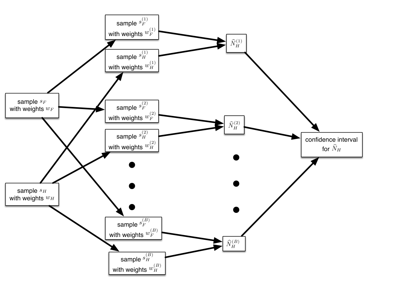
Because of the challenges involved in sampling hard-to-reach populations, the two most likely sampling designs for $s_{H}$ will be time-location sampling and respondent-driven sampling. If $s_{H}$ was selected with time-location sampling, we recommend treating the design as a two-stage element sample (see Karon and Wejnert, (2012)) and using the procedure of Rust and Rao (1996). If $s_{H}$ was selected with respondent-driven sampling, as was done in a recent study of heavy drug users in Curitiba, Brazil (Salganik et al., 2011b, ), we recommend using the best available bootstrap method for respondent-driven sampling data, which at the present time is the procedure introduced in Salganik, (2006). One implementation detail of that particular bootstrap procedure is that it requires researchers to divide the sample of the hidden population into two mutually exclusive groups. In this case, we recommend dividing the hidden population into those who are above and below the median of their estimated visibility $\widehat{v}_{i,F}$ in order to capture some of the extra uncertainty introduced if there are strong tendencies for more hidden members of the hidden population to recruit each other.

Because the generalized scale-up estimator has never been used for groups of known size, we cannot explore the coverage rate of the proposed procedure. However, based on experience with respondent-driven sampling, we suspect that variance estimation procedures for hidden populations will underestimate the actual uncertainty in the estimates (Goel and Salganik,, 2009; Goel and Salganik,, 2010; Yamanis et al.,, 2013; Verdery et al.,, 2013; Rohe,, 2015). If this is the case, then the intervals around the generalized scale-up estimates will be anti-conservative.

In conclusion, Sec. F.1 presents a bootstrap procedure for simple and complex sample designs from the sampling frame, and Sec. F.2 extends these results to account for the sampling variability introduced by having a sample from the hidden population. We have shown that the performance of these procedures on three real scale-up datasets is consistent with theoretical expectations. Additional research in this area, which is beyond the scope of this paper, could adopt a total survey error approach and attempt to quantify all sources of uncertainty in the estimates, not just sampling uncertainty. Additional research could also explore the properties and sensitivity of these confidence interval procedures though simulation.

Appendix G Simulation study

In this appendix, we describe a simulation study comparing the performance of the generalized and basic network scale-up estimators. The results of these simulations confirm and illustrate several of the analytical results in Section 3 of the paper. Most importantly, the simulations show that the generalized network scale-up estimator is unbiased for all of the situations explored by the simulation, while the basic network scale-up estimator is biased for all but a few special cases. Moreover, our analytical results correctly predict the bias of the basic network scale-up estimator in each case.

Our simulation study is intentionally simple in order to clearly illustrate our analytical results; it is not designed to be a realistic model of any scale-up study. Concretely, our simulations compare the performance of generalized and basic scale-up estimators as three important quantities vary: (1) the size of the frame population $F$ , relative to the size of the entire population, $U$ ; (2) the extent to which people’s network connections are not formed completely at random, also called the amount of inhomogenous mixing; and (3) the accuracy of reporting, as captured by the true positive rate $\tau_{F}$ (see Equation 18).

We simulate populations consisting of $N=5,000$ people, using a stochastic block-model (White et al.,, 1976; Wasserman and Faust,, 1994) to randomly generate networks with different amounts of inhomogenous mixing. Stochastic block models assume population members can be grouped into different blocks. For any pair of people, $i$ and $j$ , the probability that there is an edge between $i$ and $j$ is completely determined by the block memberships of $i$ and $j$ .

In our simulation model, each person can be either in or out of the frame population $F$ and each person can also be either in or out of the hidden population $H$ , producing four possible blocks: $FH$ , $F\lnot H$ , $\lnot F\lnot H$ , and $\lnot FH$ . (Here, we use the logical negation symbol, $\lnot$ , to denote not being in a group.) The probability of an edge between any two people $i$ and $j$ is then governed by a Bernoulli distribution whose mean is a function of the two block memberships:

\text{Pr}(i\leftrightarrow j)\sim\text{Bernoulli}(\mu_{g(i),g(j)}),

(G.1)

where $g(i)$ is the block containing $i$ , $g(j)$ is the block containing $j$ , $i\leftrightarrow j$ denotes an undirected edge between $i$ and $j$ , and $\mu_{g(i),g(j)}$ is the probability of an edge between a member of group $g(i)$ and a member of group $g(j)$ . In a network with a no inhomogenous mixing (equivalent to an Erdos-Renyi random graph), $\mu_{g(i),g(j)}$ will be the same for all $i$ and $j$ . On the other hand, in a network with a high level of inhomogenous mixing, $\mu_{g(i),g(j)}$ will be relatively small when $g(i)\neq g(j)$ and $\mu_{g(i),g(j)}$ will be relatively large when $g(i)=g(j)$ ¹⁵¹⁵ 15 Computer code to perform the simulations was written in R (R Core Team,, 2014) and used the following packages: devtools (Wickham and Chang,, 2013); functional (Danenberg,, 2013); ggplot2 (Wickham,, 2009); igraph (Csardi and Nepusz,, 2006); networkreporting (Feehan and Salganik,, 2014); plyr (Wickham,, 2011); sampling (Tillé and Matei,, 2015); and stringr (Wickham,, 2012)..

Each random network drawn under our simulation model depends on seven parameters. The first four parameters describe population size and group memberships; they are:

•

$N$ , the size of the population
•

$p_{F}$ , the fraction of people in the frame population
•

$p_{H}$ , the fraction of people in the hidden population
•

$p_{F|H}$ , the fraction of hidden population members also in the frame population

The next three parameters govern the amount of inhomogenous mixing in the network that connects people to each other; they are:

•

${\zeta}$ , the probability of an edge between two people who are both in the same block.
•

$\xi$ , the relative probability of an edge between two vertices that differ in frame population membership. For example, a value of 0.6 would mean that the chances of having a connection between a particular person in $F$ and a particular person not in $F$ is 60% of the chance of a connection between two members of $F$ or two members of $\lnot F$ .
•

$\rho$ , the relative probability of an edge between two vertices that differ in hidden population membership. For example, a value of 0.8 would mean that the chances of having a connection between a particular person in $H$ and a particular person not in $H$ is 80% of the chance of a connection between two members of $H$ or two members of $\lnot H$ .

Together, the parameters $\zeta$ , $\xi$ , and $\rho$ are used to construct the mixing matrix M (Figure G.1). Note that varying the parameter $\rho$ will change several structural features of the network in addition to the amount of inhomogenous mixing; for example, changing $\rho$ will alter the degree distribution. Our analytical results show that the generalized network scale-up estimator is robust to changes in these structural features.

\mathbf{M}=\bordermatrix{&~F~H&~F\lnot H&\lnot F~H&\lnot F\lnot H\cr~F~H&\zeta&\rho\cdot\zeta&\xi\cdot\zeta&\xi\cdot\rho\cdot\zeta\cr~F\lnot H&\rho\cdot\zeta&\zeta&\xi\cdot\rho\cdot\zeta&\xi\cdot\zeta\cr\lnot F~H&\xi\cdot\zeta&\xi\cdot\rho\cdot\zeta&\zeta&\rho\cdot\zeta\cr\lnot F\lnot H&\xi\cdot\rho\cdot\zeta&\xi\cdot\zeta&\rho\cdot\zeta&\zeta}

(G.2)

Figure G.1: The mixing matrix used to generate a random network using the stochastic block model. Entry

(i,j

) in the matrix describes the probability of an edge between two people, one of whom is in group

i

and one in group

j

. The probabilities are governed by

\zeta

\xi

, and

\rho

. In our simulations, we generate networks with different amounts of inhomogenous mixing between hidden population members and non-hidden population members by fixing

\zeta=0.05

and

\xi=0.4

, and then varying

\rho

from 0.1 (extreme inhomogenous mixing between hidden and non-hidden population members) to 1 (perfectly random mixing between hidden and non-hidden population members).

The final parameter, $\tau_{F}$ , is used to control the amount of imperfect reporting. After randomly drawing a network using the stochastic block model, we generate a reporting network as follows:

1.

convert all undirected edges $i\leftrightarrow j$ in the social network into two directed reporting edges in the reporting network: one $i\rightarrow j$ and one $j\rightarrow i$
2.

select a fraction, $1-\tau_{F}$ , of the edges that lead from members of the frame population to members of the hidden population uniformly at random and remove them from the reporting graph.

Given a simple random sample of 500 members of the frame population and a relative probability sample of 30 members of the hidden population, the reporting graph is then used to compute the basic and generalized scale-up estimates for the size of the hidden population.

Across our simulations, we fix five of the parameters at constant values ( $N=5,000$ ; $p_{F}=0.03$ ; $p_{F|H}=1$ ; $\zeta=0.05$ ; $\xi=0.4$ ). We systematically explore varying the remaining parameters: we investigate $\rho$ for values from 0.1 to 1 in increments of $0.1$ ; we investigate $p_{F}$ for values 0.1, 0.5, and 1; and we investigate $\tau_{F}$ for 0.1, 0.5, and 1. For each combination of the parameter values, we generate 10 random networks. Within each random network, we simulate 500 surveys. Each survey consists of two samples: a probability sample from the frame population, with sample size of 500; and a relative probability from the hidden population of size 30, with inclusion proportional to each hidden population member’s personal network size. For each unique combination of parameters, we averaged the results across the surveys and across the randomly generated networks.

Abstract

1 Introduction

2 The generalized scale-up estimator

2.1 Estimating NHN_{H} from sampled data

3 Comparison between the generalized and basic scale-up approaches

3.1 Illustrative simulation

4 Recommendations for practice

4.1 Estimation with samples from FF and HH

4.2 Estimation with only a sample from FF

5 Conclusion and next steps

References

Online Appendices

Appendix A Estimation in the presence of false positive reports

Appendix B Estimates with a sample from FF

B.1 Requirements for sampling designs from F

B.2 Estimating the total number of out-reports, yF,Hy_{F,H}

Result \the\csnameresultctr\endcsname

B.3 Reporting about multisets

Property \the\csnamepropertyctr\endcsname

B.4 Network degree and the known population method for estimating d¯F,F\bar{d}_{F,F}, d¯F,U\bar{d}_{F,U}, and d¯U,F\bar{d}_{U,F}

B.4.1 Guidance for choosing the probe alters, 𝒜\mathcal{A}

B.4.2 The known population estimators

Result \the\csnameresultctr\endcsname

Result \the\csnameresultctr\endcsname

Corollary \the\csnamecorctr\endcsname

B.5 Estimating the frame ratio, ϕF\phi_{F}

Result \the\csnameresultctr\endcsname

Appendix C Estimates with samples from FF and HH

C.1 Requirements for sampling designs from H

C.2 Data collection

C.3 Estimation using aggregated relational data from the hidden population

Property \the\csnamepropertyctr\endcsname

C.4 Estimating the average visibility, v¯H,F\bar{v}_{H,F}

Result \the\csnameresultctr\endcsname

Definition \the\csnamedefnctr\endcsname

Definition \the\csnamedefnctr\endcsname

Result \the\csnameresultctr\endcsname

Result \the\csnameresultctr\endcsname

C.5 Guidance for choosing the probe alters for the game of contacts, 𝒜\mathcal{A}

C.6 Term-by-term: δF\delta_{F} and τF\tau_{F}

Result \the\csnameresultctr\endcsname

C.6.1 Estimating the degree ratio, δF\delta_{F}

Result \the\csnameresultctr\endcsname

C.6.2 Estimating the true positive rate, τF\tau_{F}

Result \the\csnameresultctr\endcsname

C.7 Estimating the size of the hidden population, NHN_{H}

Result \the\csnameresultctr\endcsname

Result \the\csnameresultctr\endcsname

Result \the\csnameresultctr\endcsname

Result \the\csnameresultctr\endcsname

Appendix D Sensitivity analysis

D.1 Sensitivity to non-sampling conditions: survey construction, reporting behavior, and network structure

Result \the\csnameresultctr\endcsname

D.2 Sensitivity to sampling problems

D.2.1 Probability samples

Imperfect sampling weights.

Result \the\csnameresultctr\endcsname

Corollary \the\csnamecorctr\endcsname

D.2.2 Relative probability samples

Imperfect relative sampling weights.

Result \the\csnameresultctr\endcsname

Corollary \the\csnamecorctr\endcsname

D.2.3 Summary and results for all estimators

D.3 Combined sensitivity results

D.3.1 Generalized scale-up

Result \the\csnameresultctr\endcsname

Result \the\csnameresultctr\endcsname

Corollary \the\csnamecorctr\endcsname

D.3.2 Modified basic scale-up

Result \the\csnameresultctr\endcsname

Result \the\csnameresultctr\endcsname

Corollary \the\csnamecorctr\endcsname

Appendix E Approximate unbiasedness of compound ratio estimators

E.1 Overview

E.2 The general case

Result \the\csnameresultctr\endcsname

E.3 Applying Result E.2 to scale-up

Appendix F Variance estimation and confidence intervals

F.1 Variance estimation with a sample from FF

F.2 Variance estimation with sample from FF and HH

2.1 Estimating $N_{H}$ from sampled data

4.1 Estimation with samples from $F$ and $H$

4.2 Estimation with only a sample from $F$

Appendix B Estimates with a sample from $F$

B.2 Estimating the total number of out-reports, $y_{F,H}$

B.4 Network degree and the known population method for estimating $\bar{d}_{F,F}$ , $\bar{d}_{F,U}$ , and $\bar{d}_{U,F}$

B.4.1 Guidance for choosing the probe alters, $\mathcal{A}$

B.5 Estimating the frame ratio, $\phi_{F}$

Appendix C Estimates with samples from $F$ and $H$

C.4 Estimating the average visibility, $\bar{v}_{H,F}$

C.5 Guidance for choosing the probe alters for the game of contacts, $\mathcal{A}$

C.6 Term-by-term: $\delta_{F}$ and $\tau_{F}$

C.6.1 Estimating the degree ratio, $\delta_{F}$

C.6.2 Estimating the true positive rate, $\tau_{F}$

C.7 Estimating the size of the hidden population, $N_{H}$

F.1 Variance estimation with a sample from $F$

F.2 Variance estimation with sample from $F$ and $H$