Andrzej J. Buras^a,b, Fulvia De Fazio^c and Jennifer Girrbach^a,b
^aTUM Institute for Advanced Study, Lichtenbergstr. 2a, D-85747 Garching, Germany
^bPhysik Department, Technische Universität München, James-Franck-Straße,
D-85747 Garching, Germany
^cIstituto Nazionale di Fisica Nucleare, Sezione di Bari, Via Orabona 4, I-70126 Bari, Italy

Abstract

The experimental value for the isospin amplitude ${\rm Re}A_{2}$ in $K\to\pi\pi$ decays has been successfully explained within the Standard Model (SM), both within large $N$ approach to QCD and by QCD lattice calculations. On the other hand within large $N$ approach the value of ${\rm Re}A_{0}$ is by at least $30\%$ below the data. While this deficit could be the result of theoretical uncertainties in this approach and could be removed by future precise QCD lattice calculations, it cannot be excluded that the missing piece in ${\rm Re}A_{0}$ comes from New Physics (NP). We demonstrate that this deficit can be significantly softened by tree-level FCNC transitions mediated by a heavy colourless $Z^{\prime}$ gauge boson with flavour violating left-handed coupling $\Delta^{sd}_{L}(Z^{\prime})$ and approximately universal flavour diagonal right-handed coupling $\Delta^{qq}_{R}(Z^{\prime})$ to quarks. The approximate flavour universality of the latter coupling assures negligible NP contributions to ${\rm Re}A_{2}$ . This property together with the breakdown of GIM mechanisms at tree-level allows to enhance significantly the contribution of the leading QCD penguin operator $Q_{6}$ to ${\rm Re}A_{0}$ . A large fraction of the missing piece in the $\Delta I=1/2$ rule can be explained in this manner for $M_{Z^{\prime}}$ in the reach of the LHC, while satisfying constraints from $\varepsilon_{K}$ , $\varepsilon^{\prime}/\varepsilon$ , $\Delta M_{K}$ , LEP-II and the LHC. The presence of a small right-handed flavour violating coupling $\Delta^{sd}_{R}(Z^{\prime})\ll\Delta^{sd}_{L}(Z^{\prime})$ and of enhanced matrix elements of $\Delta S=2$ left-right operators allows to satisfy simultaneously the constraints from ${\rm Re}A_{0}$ and $\Delta M_{K}$ , although this requires some fine-tuning. We identify quartic correlation between $Z^{\prime}$ contributions to ${\rm Re}A_{0}$ , $\varepsilon^{\prime}/\varepsilon$ , $\varepsilon_{K}$ and $\Delta M_{K}$ . The tests of this proposal will require much improved evaluations of ${\rm Re}A_{0}$ and $\Delta M_{K}$ within the SM, of $\langle Q_{6}\rangle_{0}$ as well as precise tree level determinations of $|V_{ub}|$ and $|V_{cb}|$ . We present correlations between $\varepsilon^{\prime}/\varepsilon$ , $K^{+}\rightarrow\pi^{+}\nu\bar{\nu}$ and $K_{L}\rightarrow\pi^{0}\nu\bar{\nu}$ with and without the $\Delta I=1/2$ rule constraint and generalize the whole analysis to $Z^{\prime}$ with colour ( $G^{\prime}$ ) and $Z$ with FCNC couplings. In the latter case no improvement on ${\rm Re}A_{0}$ can be achieved without destroying the agreement of the SM with the data on ${\rm Re}A_{2}$ . Moreover, this scenario is very tightly constrained by $\varepsilon^{\prime}/\varepsilon$ . On the other hand in the context of the $\Delta I=1/2$ rule $G^{\prime}$ is even more effective than $Z^{\prime}$ : it provides the missing piece in ${\rm Re}A_{0}$ for $M_{G^{\prime}}=(3.5-4.0)\,{\rm TeV}$ .

1 Introduction

The non-leptonic $K_{L}\to\pi\pi$ decays have played already for almost sixty years an important role in particle physics and were instrumental in the construction of the Standard Model (SM) and in the selection of allowed extensions of this model. The three pillars in these decays are:

•

The real parts of the amplitudes $A_{I}$ for a kaon to decay into two pions with isospin $I$ which are measured to be [1]

${\rm Re}A_{0}=27.04(1)\times 10^{-8}~\,{\rm GeV},\quad{\rm Re}A_{2}=1.210(2)\times 10^{-8}~\,{\rm GeV},$ (1)

and express the so-called $\Delta I=1/2$ rule [2, 3]

$R=\frac{{\rm Re}A_{0}}{{\rm Re}A_{2}}=22.35.$ (2)
•

The parameter $\varepsilon_{K}$ , a measure of indirect CP-violation in $K_{L}\to\pi\pi$ decays, which is found to be

$\varepsilon_{K}=2.228(11)\times 10^{-3}e^{i\phi_{\varepsilon}},$ (3)

where $\phi_{\varepsilon}=43.51(5)^{\circ}$ .
•

The ratio of the direct CP-violation and indirect CP-violation in $K_{L}\to\pi\pi$ decays measured to be [1, 4, 5, 6]

$\rm{Re}(\varepsilon^{\prime}/\varepsilon)=(16.5\pm 2.6)\times 10^{-4}.$ (4)

Also the strongly suppressed branching ratio for the rare decay $K_{L}\to\mu^{+}\mu^{-}$ and the tiny experimental value for $K_{L}-K_{S}$ mass difference

(\Delta M_{K})_{\rm exp}=3.484(6)10^{-15}\ \textrm{GeV}=5.293(9)\text{ps}^{-1}

(5)

were strong motivations for the GIM mechanism [7] and in turn allowed to predict not only the existence of the charm quark but also approximately its mass [8].

While due to the GIM mechanism $\varepsilon_{K}$ , $\varepsilon^{\prime}/\varepsilon$ and $\Delta M_{K}$ receive contributions from the SM dynamics first at one-loop level and as such are sensitive to NP contributions, the $\Delta I=1/2$ rule involving tree-level decays has been expected already for a long time to be governed by SM dynamics. Unfortunately due to non-perturbative nature of non-leptonic decays precise calculation of the amplitudes ${\rm Re}A_{0}$ and ${\rm Re}A_{2}$ do not exist even today. However, a significant progress in reaching this goal over last forty years has been made.

Indeed, after pioneering calculations of short distance QCD effects in the amplitudes ${\rm Re}A_{0}$ and ${\rm Re}A_{2}$ [9, 10], termed in the past as octet enhancement, and the discovery of QCD penguin operators [11] which in the isospin limit contribute only to ${\rm Re}A_{0}$ , the dominant dynamics behind the $\Delta I=1/2$ has been identified in [12]. To this end an analytic approximate approach based on the dual representation of QCD as a theory of weakly interacting mesons for large $N$ , advocated previously in [13, 14, 15, 16], has been used. In this approach $\Delta I=1/2$ rule for $K\to\pi\pi$ decays has a simple origin. The octet enhancement through the long but slow quark-gluon renormalization group evolution down to the scales $\mathcal{O}(1\,{\rm GeV})$ , analyzed first in [9, 10], is continued as a short but fast meson evolution down to zero momentum scales at which the factorization of hadronic matrix elements is at work. The recent inclusion of lowest-lying vector meson contributions in addition to the pseudoscalar ones and of NLO QCD corrections to Wilson coefficients in a momentum scheme improved significantly the matching between quark-gluon and meson evolutions [17]. In this approach QCD penguin operators play a subdominant role but one can uniquely predict an enhancement of ${\rm Re}A_{0}$ through QCD penguin contributions. Working at scales $\mathcal{O}(1\,{\rm GeV})$ this enhancement amounts to roughly $15\%$ of the experimental value of ${\rm Re}A_{0}$ subject to uncertainties to which we will return below.

In the present era of the dominance of non-perturbative QCD calculations by lattice simulations with dynamical fermions, that have a higher control over uncertainties than the approach in [12, 17], it is very encouraging that the structure of the enhancement of ${\rm Re}A_{0}$ and suppression of ${\rm Re}A_{2}$ , identified already in [12], has also been found by RBC-UKQCD collaboration [18, 19, 20, 21]. The comparison between the results of both approaches in [17] indicates that the experimental value of the amplitude ${\rm Re}A_{2}$ can be well described within the SM, in particular, as the calculations in these papers have been performed at rather different scales and using a different technology.

On the other hand both approaches cannot presently obtain sufficiently large value of ${\rm Re}A_{0}$ . Within the dual QCD approach one finds then $R=16.0\pm 1.5$ , while the first lattice results for ${\rm Re}A_{0}$ imply $R\approx 11$ . However, the latter result has been obtained with non-physical kinematics and it is to be expected that larger values of $R$ , even as high as its experimental value in (2), could be obtained in lattice QCD in the future.

Presently theoretical value of ${\rm Re}A_{0}$ within dual QCD approach is by $30\%$ below the data and even more in the case of lattice QCD. While this deficit could be the result of theoretical uncertainties in both approaches, it cannot be excluded that the missing piece in ${\rm Re}A_{0}$ comes from New Physics (NP). In this context we would like to emphasize, that although the explanation of the dynamics behind the $\Delta I=1/2$ rule is not any longer at the frontiers of particle physics, it is important to determine precisely the room for NP contribution left not only in ${\rm Re}A_{0}$ but also ${\rm Re}A_{2}$ . From the present perspective only lattice simulations with dynamical fermions can provide precise values of ${\rm Re}A_{0,2}$ one day, but this may still take several years of intensive efforts by the lattice community [22, 23, 24]. Having precise SM values for ${\rm Re}A_{0,2}$ would give us two observables which could be used to constrain NP. Our paper demonstrates explicitly the impact of such constraints.

In this context we would like to strongly emphasize that while the dominant part of the $\Delta I=1/2$ rule originates in the SM dynamics it is legitimate to ask whether some subleading part of it comes from much shorter distance scales and either exclude this possibility or demonstrate that this indeed could be the case under certain assumptions.

In what follows our working assumption will be that roughly $30\%$ of ${\rm Re}A_{0}$ comes from some kind of NP which does not affect ${\rm Re}A_{2}$ in order not to spoil the agreement of the SM with the data. As the missing piece in ${\rm Re}A_{0}$ is by about eight times larger than the measured value of ${\rm Re}A_{2}$ , the required NP must have a particular structure: tiny or absent contributions to ${\rm Re}A_{2}$ and at the same time large contributions to ${\rm Re}A_{0}$ . Moreover it should satisfy other constraints coming from $\varepsilon_{K}$ , $\Delta M_{K}$ , $\varepsilon^{\prime}/\varepsilon$ and rare kaon decays.

As $K\to\pi\pi$ decays originate already at tree-level, we expect that NP contributing to these decays at one-loop level will not help us in reaching our goal. Consequently we have to look for NP that contributes to $K\to\pi\pi$ decays already at tree-level as well. Moreover in order not to spoil the agreement of the SM with the data for ${\rm Re}A_{2}$ only Wilson coefficients of QCD penguin operators should be modified. In this context we recall that in [25] an additional (with respect to previous estimates) enhancement of the QCD penguin contributions to ${\rm Re}A_{0}$ has been identified. It comes from an incomplete GIM cancellation above the charm quark mass. But as the analyses in [12, 17] show, this enhancement is insufficient to reproduce fully the experimental value of ${\rm Re}A_{0}$ .

However, the observation that the breakdown of GIM mechanism and the enhanced contributions of QCD penguin operators could in principle provide the missing part of the $\Delta I=1/2$ rule, gives us a hint what kind of NP could do the job here. We have to break GIM mechanism at a much higher scale than scales $\mathcal{O}(m_{c})$ and allow the QCD renormalization group evolution to enhance the Wilson coefficient of the leading QCD penguin operator $Q_{6}$ by a larger amount than it is possible within the SM.

It turns then out that a tree-level exchange of heavy neutral gauge boson, colourless ( $Z^{\prime}$ ) or carrying colour ( $G^{\prime}$ ) can provide a significant part of the missing piece of ${\rm Re}A_{0}$ but the couplings of these heavy gauge bosons to SM fermions must have a very special structure in order to satisfy existing constraints from other observables. Assuming $M_{Z^{\prime}}(M_{G^{\prime}})$ to be in the ballpark of a few $\,{\rm TeV}$ and denoting left-handed (LH) and right-handed (RH) couplings of $Z^{\prime}(G^{\prime})$ to two SM fermions with flavours $i$ and $j$ , as in [26], by $\Delta_{L,R}^{ij}(Z^{\prime})$ , we find that in the mass eigenstate basis for all particles involved, a $Z^{\prime}$ or $G^{\prime}$ with the following general structure of its couplings is required:

•

${\rm Re}\Delta_{L}^{sd}(Z^{\prime})=\mathcal{O}(1)$ and ${\rm Re}\Delta_{R}^{qq}(Z^{\prime})=\mathcal{O}(1)$ in order to generate $Q_{6}$ penguin operator with sizable Wilson coefficient in the presence of a heavy $Z^{\prime}$ .
•

The diagonal couplings $\Delta_{R}^{qq}(Z^{\prime})$ must be flavour universal in order not to affect the amplitude ${\rm Re}A_{2}$ . But this universality cannot be exact as this would not allow to generate a small ${\rm Re}\Delta_{R}^{sd}(Z^{\prime})=\mathcal{O}(10^{-3})$ coupling which is required in order to satisfy the constraint on $\Delta M_{K}$ in the presence of ${\rm Re}\Delta_{L}^{sd}(Z^{\prime})=\mathcal{O}(1)$ .
•

${\rm Im}\Delta_{L}^{sd}(Z^{\prime})$ and ${\rm Im}\Delta_{R}^{qq}(Z^{\prime})$ must be typically $\mathcal{O}(10^{-3}-10^{-4})$ in order to be consistent with the data on $\varepsilon_{K}$ and $\varepsilon^{\prime}/\varepsilon$ .
•

The couplings to leptons must be sufficiently small in order not to violate the existing bounds on rare kaon decays. This is automatically satisfied for $G^{\prime}$ .
•

Finally, $\Delta_{L}^{uu}(Z^{\prime})$ must be small in order not to generate large contributions to the current-current operators $Q_{1}$ and $Q_{2}$ that could affect the amplitude ${\rm Re}A_{2}$ .

We observe, that indeed the structure of the $Z^{\prime}$ or $G^{\prime}$ couplings must be rather special. But in the context of $\varepsilon^{\prime}/\varepsilon$ it is interesting to note that in this NP scenario, as opposed to many NP scenarios, there is no modification of Wilson coefficients of electroweak penguin operators up to tiny renormalization group effects that can be neglected for all practical purposes. NP part of $\varepsilon^{\prime}/\varepsilon$ involves only QCD penguin operators, in particular $Q_{6}$ , and the size of this effect, as we will demonstrate below, is correlated with NP contribution to ${\rm Re}A_{0}$ , $\varepsilon_{K}$ and $\Delta M_{K}$ .

Now comes an important point. While SM contribution to ${\rm Re}A_{0}$ practically does not involve any CKM uncertainties, this is not the case of $\varepsilon_{K}$ , $\varepsilon^{\prime}/\varepsilon$ and branching ratios on rare kaon decays which all involve potential uncertainties due to present inaccurate knowledge of the elements of the CKM matrix $|V_{ub}|$ and $|V_{cb}|$ . Therefore there are uncertainties in the room left for NP in these observables and these uncertainties in turn affect indirectly the allowed size of NP contribution to ${\rm Re}A_{0}$ . Therefore it will be of interest to consider several scenarios for the pair $|V_{ub}|$ and $|V_{cb}|$ and investigate in each case whether $Z^{\prime}$ couplings required to improve the situation with the $\Delta I=1/2$ rule could also help in explaining the data on $\varepsilon_{K}$ , $\varepsilon^{\prime}/\varepsilon$ , $\Delta M_{K}$ and rare kaon decays in case the SM would fail to do it one day. Of course presently one cannot reach clear cut conclusions on these matters due to hadronic uncertainties affecting $\varepsilon_{K}$ , $\varepsilon^{\prime}/\varepsilon$ and $\Delta M_{K}$ but it is expected that the situation will improve in this decade.

In order to be able to discuss implications for $K^{+}\rightarrow\pi^{+}\nu\bar{\nu}$ and $K_{L}\rightarrow\pi^{0}\nu\bar{\nu}$ we will assume in the first part of our paper that $Z^{\prime}$ is colourless. This is also the case analyzed in all our previous $Z^{\prime}$ papers [27, 26, 28, 29, 30, 31, 32, 33]. Subsequently, we will discuss how our analysis changes in the case of $G^{\prime}$ . The fact that in this case $G^{\prime}$ does not contribute to $K^{+}\rightarrow\pi^{+}\nu\bar{\nu}$ and $K_{L}\rightarrow\pi^{0}\nu\bar{\nu}$ allows already to distinguish this case from the colourless $Z^{\prime}$ but also the LHC bounds on the couplings of such bosons and the NP contributions to ${\rm Re}A_{0}$ , $\varepsilon^{\prime}/\varepsilon$ , $\varepsilon_{K}$ and $\Delta M_{K}$ are different in these two cases. In our presentation we will also first assume exact flavour universality for $\Delta_{R}^{qq}(Z^{\prime})$ and $\Delta_{R}^{qq}(G^{\prime})$ couplings in order to demonstrate that in this case the experimental constraints from ${\rm Re}A_{0}$ and $\Delta M_{K}$ cannot be simultaneously satisfied. Fortunately already a very small violation of flavour universality in $\Delta_{R}^{qq}(Z^{\prime})$ or $\Delta_{R}^{qq}(G^{\prime})$ allows to cure this problem because of the enhanced matrix elements of left-right operators contributing in this case to $\Delta M_{K}$ .

Our paper is organized as follows. In Section 2 we briefly describe some general aspects of $Z^{\prime}$ and $G^{\prime}$ models considered by us. In Section 3 we present general formulae for the effective Hamiltonian for $K\to\pi\pi$ decays including all operators, list the initial conditions for Wilson coefficients at $\mu=M_{Z^{\prime}}$ for the case of a colourless $Z^{\prime}$ and find the expressions for ${\rm Re}A_{0}$ and $\varepsilon^{\prime}/\varepsilon$ that include SM and $Z^{\prime}$ contributions. In Section 4 we discuss briefly $\varepsilon_{K}$ , $\Delta M_{K}$ , $K^{+}\rightarrow\pi^{+}\nu\bar{\nu}$ and $K_{L}\rightarrow\pi^{0}\nu\bar{\nu}$ , again for a colourless $Z^{\prime}$ , referring for details to our previous papers. In Section 5 we present numerical analysis of ${\rm Re}A_{0}$ , $\varepsilon^{\prime}/\varepsilon$ and $K^{+}\rightarrow\pi^{+}\nu\bar{\nu}$ and $K_{L}\rightarrow\pi^{0}\nu\bar{\nu}$ taking into account the constraints from $\varepsilon_{K}$ and $\Delta M_{K}$ . We consider two scenarios. One in which we impose the $\Delta I=1/2$ constraint (Scenario A) and one in which we ignore this constraint (Scenario B). These two scenarios can be clearly distinguished through the rare decays $K^{+}\rightarrow\pi^{+}\nu\bar{\nu}$ and $K_{L}\rightarrow\pi^{0}\nu\bar{\nu}$ and their correlation with $\varepsilon^{\prime}/\varepsilon$ . In Section 6 we repeat the full analysis for $G^{\prime}$ and in Section 7 for the $Z$ boson with flavour violating couplings. We conclude in Section 8.

2 General Aspects of $Z^{\prime}$ and $G^{\prime}$ Models

The present paper is the continuation of our extensive study of NP represented by a new neutral heavy gauge boson ( $Z^{\prime}$ ) in the context of a general parametrization of its couplings to SM fermions and within specific models like 331 models [27, 26, 28, 29, 30, 31, 32, 33]. The new aspect of the present paper is the generalization of these studies to $K\to\pi\pi$ decays with the goal to answer three questions:

•

Whether the existence of a $Z^{\prime}$ or $G^{\prime}$ with a mass in the reach of the LHC could have an impact on the $\Delta I=1/2$ rule, in particular on the amplitude ${\rm Re}A_{0}$ .
•

Whether such gauge bosons could have sizable impact on the ratio $\varepsilon^{\prime}/\varepsilon$ .
•

What is the impact of $\varepsilon^{\prime}/\varepsilon$ constraint on FCNC couplings of the SM $Z$ boson.

To our knowledge the first question has not been addressed in the literature, while selected analyses of $\varepsilon^{\prime}/\varepsilon$ within models with tree-level flavour changing neutral currents can be found in [34, 35]. However, in these papers NP entered $\varepsilon^{\prime}/\varepsilon$ through electroweak penguin operators while in the case of $Z^{\prime}$ scenarios considered here only QCD penguin operators are relevant. Concerning the last point we refer to earlier analyses in [36, 37]. The present paper provides a modern look at this scenario and in particular investigates the sensitivity to CKM parameters. A review of $Z^{\prime}$ models can be found in [38] and a collection of papers related mainly to $B_{s,d}$ decays can be found in [26].

Our paper will deal with NP in $K^{0}-\bar{K}^{0}$ mixing, $K\to\pi\pi$ and rare $K$ decays dominated either by a heavy $Z^{\prime}$ , heavy $G^{\prime}$ or FCNC processes mediated by $Z$ . We will not provide a complete model in which other fields like heavy vector-like fermions, heavy Higgs scalars and charged gauge bosons are generally present and gauge anomalies are properly canceled. Examples of such models can be found in [38] and the 331 models analyzed by us can be mentioned here [27, 33]. A general discussion can also be found in [39] and among more recent papers we refer to [40] and [41]. But none of these papers discusses the hierarchy of the couplings of $Z^{\prime}$ and $G^{\prime}$ couplings which is required to make these gauge bosons to be relevant for the $\Delta I=1/2$ rule. Our goal then is to find this hierarchy first and postpone the construction of a concrete model to a future analysis.

$Z^{\prime}$ contributions to ${{\rm{Re}}A_{0}}$ , ${{\rm{Re}}A_{2}}$ and $\varepsilon^{\prime}/\varepsilon$ involve generally in addition to $M_{Z^{\prime}}$ the following couplings:

\Delta_{L}^{sd}(Z^{\prime}),\hskip 22.99988pt\Delta_{R}^{sd}(Z^{\prime}),\hskip 22.99988pt\Delta_{L}^{qq}(Z^{\prime}),\hskip 22.99988pt\Delta_{R}^{qq}(Z^{\prime}),

(6)

where $q=u,d,c,s,b,t$ . The same applies to $G^{\prime}$ . The diagonal couplings can be generally flavour dependent but as we already stated above in order to protect the small amplitude ${{\rm{Re}}A_{2}}$ from significant NP contributions in the process of modification of the large amplitude ${{\rm{Re}}A_{0}}$ either the coupling $\Delta_{L}^{qq}(Z^{\prime})$ or the coupling $\Delta_{R}^{qq}(Z^{\prime})$ must be approximately flavour universal. They cannot be both flavour universal as then it would not be possible to generate large flavour violating couplings in the mass eigenstate basis. In what follows we will assume that $\Delta_{R}^{qq}(Z^{\prime})$ are either exactly flavour universal or flavour universal to a high degree still allowing for a strongly suppressed but non-vanishing coupling $\Delta_{R}^{sd}(Z^{\prime})$ .

For the left-handed couplings it will turn out that $\Delta_{L}^{sd}(Z^{\prime})=\mathcal{O}(1)$ in order to reach the first goal on our list. Such a coupling could be in principle generated in the presence of heavy vectorial fermions or other dynamics at scales above $M_{Z^{\prime}}$ . In order to simplify our analysis and reduce the number of free parameters, we will finally assume that $\Delta_{L}^{qq}(Z^{\prime})$ are very small. Thus in summary the hierarchy of couplings in the present paper will be assumed to be as follows:

\Delta_{L}^{sd}(Z^{\prime})\gg\Delta_{L}^{qq}(Z^{\prime}),\hskip 22.99988pt\Delta_{R}^{sd}(Z^{\prime})\ll\Delta_{R}^{qq}(Z^{\prime}),\hskip 22.99988pt\Delta_{L}^{sd}(Z^{\prime})\gg\Delta_{R}^{sd}(Z^{\prime})

(7)

with the same hierarchy assumed for $G^{\prime}$ .

Only the coupling $\Delta_{L,R}^{sd}(Z^{\prime})$ will be assumed to be complex while as we will see in the context of our analysis the remaining two can be assumed to be real without particular loss of generality. We should note that the hierarchy in (7) will suppress in the case of $K\to\pi\pi$ decays the primed operators that are absent in the SM anyway.

In our previous papers we have considered a number of scenarios for flavour violating $Z^{\prime}$ couplings to quarks. These are defined as follows:

1.

Left-handed Scenario (LHS) with complex $\Delta_{L}^{sd}\not=0$ and $\Delta_{R}^{sd}=0$ ,
2.

Right-handed Scenario (RHS) with complex $\Delta_{R}^{sd}\not=0$ and $\Delta_{L}^{sd}=0$ ,
3.

Left-Right symmetric Scenario (LRS) with complex $\Delta_{L}^{sd}=\Delta_{R}^{sd}\not=0$ ,
4.

Left-Right asymmetric Scenario (ALRS) with complex $\Delta_{L}^{sd}=-\Delta_{R}^{sd}\not=0$ .

Among them only LHS scenario is consistent with (7) if $\Delta_{R}^{sd}$ is assumed to vanish. But as we will demonstrate in this case it is not possible to satisfy simultaneously the constraints from ${{\rm{Re}}A_{0}}$ and $\Delta M_{K}$ . Consequently $\Delta_{R}^{sd}$ has to be non-vanishing, although very small, in order to satisfy these two constraints simultaneously. Thus in the scenarios considered in our previous papers the status of the $\Delta I=1/2$ rule cannot be improved with respect to the SM.

3 General Formulae for $K\to\pi\pi$ Decays

3.1 General Structure

Let us begin our presentation with the general formula for the effective Hamiltonian relevant for $K\to\pi\pi$ decays in the model in question

\mathcal{H}_{\rm eff}(K\to\pi\pi)=\mathcal{H}_{\rm eff}(K\to\pi\pi)({\rm SM})+\mathcal{H}_{\rm eff}(K\to\pi\pi)(Z^{\prime})

(8)

where the SM part is given by [42]

\mathcal{H}_{\rm eff}(K\to\pi\pi)({\rm SM})=\frac{G_{F}}{\sqrt{2}}V_{ud}V_{us}^{*}\sum_{i=1}^{10}(z^{\rm SM}_{i}(\mu)+\tau y^{\rm SM}_{i}(\mu))Q_{i},\hskip 22.99988pt\tau=-\frac{V_{td}V_{ts}^{*}}{V_{ud}V_{us}^{*}},

(9)

and the operators $Q_{i}$ as follows:

Current–Current:

Q_{1}=(\bar{s}_{\alpha}u_{\beta})_{V-A}\;(\bar{u}_{\beta}d_{\alpha})_{V-A}~~~~~~Q_{2}=(\bar{s}u)_{V-A}\;(\bar{u}d)_{V-A}

(10)

QCD–Penguins:

Q_{3}=(\bar{s}d)_{V-A}\sum_{q=u,d,s,c,b,t}(\bar{q}q)_{V-A}~~~~~~Q_{4}=(\bar{s}_{\alpha}d_{\beta})_{V-A}\sum_{q=u,d,s,c,b,t}(\bar{q}_{\beta}q_{\alpha})_{V-A}

(11)

Q_{5}=(\bar{s}d)_{V-A}\sum_{q=u,d,s,c,b,t}(\bar{q}q)_{V+A}~~~~~Q_{6}=(\bar{s}_{\alpha}d_{\beta})_{V-A}\sum_{q=u,d,s,c,b,t}(\bar{q}_{\beta}q_{\alpha})_{V+A}

(12)

Electroweak Penguins:

Q_{7}=\frac{3}{2}\;(\bar{s}d)_{V-A}\sum_{q=u,d,s,c,b,t}e_{q}\;(\bar{q}q)_{V+A}~~~~~Q_{8}=\frac{3}{2}\;(\bar{s}_{\alpha}d_{\beta})_{V-A}\sum_{q=u,d,s,c,b,t}e_{q}(\bar{q}_{\beta}q_{\alpha})_{V+A}

(13)

Q_{9}=\frac{3}{2}\;(\bar{s}d)_{V-A}\sum_{q=u,d,s,c,b,t}e_{q}(\bar{q}q)_{V-A}~~~~~Q_{10}=\frac{3}{2}\;(\bar{s}_{\alpha}d_{\beta})_{V-A}\sum_{q=u,d,s,c,b,t}e_{q}\;(\bar{q}_{\beta}q_{\alpha})_{V-A}

(14)

Here, $\alpha,\beta$ denote colours and $e_{q}$ denotes the electric quark charges reflecting the electroweak origin of $Q_{7},\ldots,Q_{10}$ . Finally, $(\bar{s}d)_{V-A}\equiv\bar{s}_{\alpha}\gamma_{\mu}(1-\gamma_{5})d_{\alpha}$ .

The coefficients $z^{\rm SM}_{i}(\mu)$ and $y^{\rm SM}_{i}(\mu)$ are the Wilson coefficients of these operators within the SM. They are known at the NLO level in the renormalization group improved perturbation theory including both QCD and QED corrections [42, 43]. Also some elements of NNLO corrections can be found in the literature [44, 45].

As discussed in the previous section $Z^{\prime}$ contributions to $K\to\pi\pi$ in the class of $Z^{\prime}$ models discussed by us can be well approximated by the following effective Hamiltonian

\mathcal{H}_{\rm eff}(K\to\pi\pi)(Z^{\prime})=\sum_{i=3}^{6}(C_{i}(\mu)Q_{i}+C_{i}^{\prime}(\mu)Q_{i}^{\prime}),

(15)

where the primed operators $Q_{i}^{\prime}$ are obtained from $Q_{i}$ by interchanging $V-A$ and $V+A$ . For the sake of completeness we keep still $Q_{i}^{\prime}$ operators even if at the end due to the hierarchy of couplings in (7), $Z^{\prime}$ contributions will be well approximated by $Q_{i}$ and the contributions from $Q_{i}^{\prime}$ operators can be neglected.

Due to the fact that $M_{Z^{\prime}}\gg m_{t}$ the summation over flavours in (11)-(14) includes now also the top quark. This structure is valid for both $Z^{\prime}$ and $G^{\prime}$ . As the hadronic matrix elements of $Q_{i}$ do not depend on the properties of $Z^{\prime}$ or $G^{\prime}$ , these two cases can only be distinguished by the values of the coefficients $C_{i}(\mu)$ and $C_{i}^{\prime}(\mu)$ . In this and two following sections we analyze the case of $Z^{\prime}$ . But in Section 6 we will also discuss $G^{\prime}$ .

The important feature of the effective Hamiltonian in (15) is the absence of $Q_{1,2}$ operators dominating the $A_{2}$ amplitude and the absence of electroweak penguin operators which in some of the extensions of the SM are problematic for $\varepsilon^{\prime}/\varepsilon$ . In our model NP effects in ${\rm Re}A_{0}$ , relevant for the $\Delta I=1/2$ rule and ${\rm Im}A_{0}$ , relevant for $\varepsilon^{\prime}/\varepsilon$ , will enter only through QCD penguin contributions. This is a novel feature when compared with other scenarios, like LHT [46] and Randall-Sundrum scenarios [34, 35], where NP contributions to $\varepsilon^{\prime}/\varepsilon$ are dominated by electroweak penguin operators. In particular, in the latter case, where FCNCs are mediated by new heavy Kaluza-Klein gauge bosons, the flavour universality of their diagonal couplings to quarks is absent due to different positions of light and heavy quarks in the bulk. Consequently the pattern of NP contributions to $\varepsilon^{\prime}/\varepsilon$ differs from the one in the models discussed here.

Denoting by $\Delta_{L,R}^{ij}$ , as in [26], the couplings of $Z^{\prime}$ to two quarks with flavours $i$ and $j$ , a tree level $Z^{\prime}$ exchange generates in our model only the operators $Q_{3}$ , $Q_{5}$ , $Q^{\prime}_{3}$ and $Q^{\prime}_{5}$ at $\mu=M_{Z^{\prime}}$ . The inclusion of QCD effects, in particular the renormalization group evolution down to low energy scales, generates the remaining QCD penguin operators. In principle using the two-loop anomalous dimensions of [42, 43] and the $\mathcal{O}(\alpha_{s})$ corrections to the coefficients $C_{i}$ and $C_{i}^{\prime}$ at $\mu_{Z^{\prime}}=\mathcal{O}(M_{Z^{\prime}})$ in the NDR- ${\rm\overline{MS}}$ scheme in [47] the full NLO analysis of $Z^{\prime}$ contributions could be performed. However, due to the fact that the mass of $Z^{\prime}$ is free and other parametric and hadronic uncertainties, a leading order analysis of NP contributions is sufficient for our purposes. In this manner it will also be possible to see certain properties analytically.

The non-vanishing Wilson coefficients at $\mu=M_{Z^{\prime}}$ are then given at the LO as follows

	$\displaystyle\begin{split}C_{3}(M_{Z^{\prime}})&=\frac{\Delta_{L}^{sd}(Z^{\prime})\Delta_{L}^{qq}(Z^{\prime})}{4M^{2}_{Z^{\prime}}},\hskip 22.99988ptC_{3}^{\prime}(M_{Z^{\prime}})=\frac{\Delta_{R}^{sd}(Z^{\prime})\Delta_{R}^{qq}(Z^{\prime})}{4M^{2}_{Z^{\prime}}}\,,\end{split}$			(16)
	$\displaystyle\begin{split}C_{5}(M_{Z^{\prime}})&=\frac{\Delta_{L}^{sd}(Z^{\prime})\Delta_{R}^{qq}(Z^{\prime})}{4M^{2}_{Z^{\prime}}},\hskip 22.99988ptC_{5}^{\prime}(M_{Z^{\prime}})=\frac{\Delta_{R}^{sd}(Z^{\prime})\Delta_{L}^{qq}(Z^{\prime})}{4M^{2}_{Z^{\prime}}}\,.\end{split}$			(17)

3.2 Renormalization Group Analysis (RG)

With these results at hand we will perform RG analysis of NP contributions at the LO level¹¹ 1 SM contributions are evaluated including NLO QCD corrections.. We will then see that the only operator that matters at scales $\mathcal{O}(1\,{\rm GeV})$ in our $Z^{\prime}$ models is either $Q_{6}$ or $Q_{6}^{\prime}$ . This is to be expected if we recall that at $\mu=M_{W}$ the Wilson coefficient of the electroweak penguin operator $Q_{8}$ , the electroweak analog of $Q_{6}$ , also vanishes. But due to its large anomalous dimension and enhanced hadronic $K\to\pi\pi$ matrix elements $Q_{8}$ is by far the dominant electroweak penguin operator in $\varepsilon^{\prime}/\varepsilon$ within the SM, leaving behind the $Q_{7}$ operator whose Wilson coefficient does not vanish at $\mu=M_{W}$ . Even if the structure of the present RG analysis differs from the SM one, due to the absence of the remaining operators in the NP part, in particular the absence of $Q_{2}$ , much longer RG evolution from $M_{Z^{\prime}}$ and not $M_{W}$ down to low energies makes $Q_{6}$ or $Q_{6}^{\prime}$ the winner at the end. This fact as we will see simplifies significantly the phenomenological analysis of NP contributions to ${\rm Re}A_{0}$ and $\varepsilon^{\prime}/\varepsilon$ .

The relevant $4\times 4$ one-loop anomalous dimension matrix

\hat{\gamma}_{s}(\alpha_{s})=\hat{\gamma}_{s}^{(0)}\frac{\alpha_{s}}{4\pi}

(18)

can be extracted from the known $6\times 6$ matrix [48]. The evolution of the operators in the NP part is then governed in the $(Q_{3},Q_{4},Q_{5},Q_{6})$ basis by

\hat{\gamma}^{(0)}_{s}=\left(\begin{array}[]{cccc}\frac{-22}{9}&\frac{22}{3}&-\frac{4}{9}&\frac{4}{3}\\ \vbox{\vskip 14.22636pt}6-f\frac{2}{9}&-2+f\frac{2}{3}&-f\frac{2}{9}&f\frac{2}{3}\\ \vbox{\vskip 14.22636pt}0&0&{2}&-6\\ \vbox{\vskip 14.22636pt}-f\frac{2}{9}&f\frac{2}{3}&-f\frac{2}{9}&-16+f\frac{2}{3}\end{array}\right),

(19)

where $f$ is the number of effective flavours: $f=6$ for $\mu\geq m_{t}$ and $f=3$ for $\mu\leq m_{c}$ . The same matrix governs the evolution of primed operators.

In order to see what happens analytically we then assume first that in the mass eigenstate basis only the couplings $\Delta_{L}^{sd}$ and $\Delta_{R}^{qq}$ are non-vanishing with $\Delta_{R}^{qq}$ being exactly flavour universal. While, the coefficients of the operators $Q_{3}$ and $Q_{4}$ can still be generated through RG evolution, these effects are very small and can be neglected. Then to an excellent approximation only the operators $Q_{5}$ and $Q_{6}$ matter and RG evolution is governed by the reduced $2\times 2$ anomalous dimension matrix given in the $(Q_{5},Q_{6})$ basis as follows

\hat{\gamma}^{(0)}_{s}=\left(\begin{array}[]{cc}2&-6\\ \vbox{\vskip 14.22636pt}-f\frac{2}{9}&-16+f\frac{2}{3}\end{array}\right).

(20)

Denoting then by $\vec{C}(M_{Z^{\prime}})$ the column vector with components given by the Wilson coefficients $C_{5}$ and $C_{6}$ at $\mu=M_{Z^{\prime}}$ we find their values at $\mu=m_{c}$ by means of²² 2 The reason for choosing $\mu=m_{c}$ will be explained below.

\vec{C}(m_{c})=\hat{U}(m_{c},M_{Z^{\prime}})\vec{C}(M_{Z^{\prime}})

(21)

where

\hat{U}(m_{c},M_{Z^{\prime}})=\hat{U}^{(f=4)}(m_{c},m_{b})\hat{U}^{(f=5)}(m_{b},m_{t})\hat{U}^{(f=6)}(m_{t},M_{Z^{\prime}})

(22)

and [49]

\hat{U}^{(f)}(\mu_{1},\mu_{2})=\hat{V}\left({\left[\frac{\alpha_{s}(\mu_{2})}{\alpha_{s}(\mu_{1})}\right]}^{\frac{\vec{\gamma}^{(0)}}{2\beta_{0}}}\right)_{D}\hat{V}^{-1}.

(23)

Here $\hat{V}$ diagonalizes ${\hat{\gamma}^{(0)T}}$

\hat{\gamma}^{(0)}_{D}=\hat{V}^{-1}{\hat{\gamma}^{(0)T}}\hat{V}

(24)

and $\vec{\gamma}^{(0)}$ is the vector containing the diagonal elements of the diagonal matrix :

\hat{\gamma}^{(0)}_{D}=\left(\begin{array}[]{cc}\gamma^{(0)}_{+}&0\\ 0&\gamma^{(0)}_{-}\end{array}\right).

(25)

with

\beta_{0}=\frac{33-2f}{3}\,.

(26)

For $\alpha_{s}(M_{Z})=0.1185$ , $m_{c}=1.3\,{\rm GeV}$ and $M_{Z^{\prime}}=3\,{\rm TeV}$ we have

\left[\begin{array}[]{c}C_{5}(m_{c})\\ C_{6}(m_{c})\end{array}\right]=\left[\begin{array}[]{cc}0.86&0.19\\ 1.13&3.60\end{array}\right]\left[\begin{array}[]{c}1\\ 0\end{array}\right]\frac{\Delta_{L}^{sd}(Z^{\prime})\Delta_{R}^{qq}(Z^{\prime})}{4M^{2}_{Z^{\prime}}}.

(27)

Consequently

C_{5}(m_{c})=0.86\frac{\Delta_{L}^{sd}(Z^{\prime})\Delta_{R}^{qq}(Z^{\prime})}{4M^{2}_{Z^{\prime}}}\hskip 22.99988ptC_{6}(m_{c})=1.13\frac{\Delta_{L}^{sd}(Z^{\prime})\Delta_{R}^{qq}(Z^{\prime})}{4M^{2}_{Z^{\prime}}}.

(28)

Due to the large element $(1,2)$ in the matrix (20) and the large anomalous dimension of the $Q_{6}$ operator represented by the $(2,2)$ element of this matrix, $C_{6}(m_{c})$ is by a factor of $1.3$ larger than $C_{5}(m_{c})$ even if $C_{6}(M_{Z^{\prime}})$ vanishes at LO. Moreover the matrix element $\langle Q_{5}\rangle_{0}$ is colour suppressed which is not the case of $\langle Q_{6}\rangle_{0}$ and within a good approximation we can neglect the contribution of $Q_{5}$ . In summary, it is sufficient to keep only $Q_{6}$ contribution in the decay amplitude in this scenario for $Z^{\prime}$ couplings.

3.3 The Total $A_{0}$ Amplitude

Adding NP contributions to the SM contribution we find

A_{0}=A_{0}^{\rm SM}+A_{0}^{\rm NP},\hskip 22.99988pt

(29)

with the SM contribution given by

{\rm{Re}}A_{0}^{\rm SM}=\frac{G_{F}}{\sqrt{2}}\lambda_{u}\sum_{i=1}^{10}z^{\rm SM}_{i}(\mu)\langle Q_{i}(\mu)\rangle_{0},

(30)

{\rm{Im}}A_{0}^{\rm SM}=-\frac{G_{F}}{\sqrt{2}}{\rm{Im}}\lambda_{t}\sum_{i=3}^{10}y^{\rm SM}_{i}(\mu)\langle Q_{i}(\mu)\rangle_{0}\,.

(31)

Here

\lambda_{i}=V_{id}V_{is}^{*}

(32)

is the usual CKM factor. As NP enters only Wilson coefficients and

\langle Q^{\prime}_{i}(\mu)\rangle_{0}=-\langle Q_{i}(\mu)\rangle_{0},

(33)

NP contributions can be included by modifying $z_{i}$ and $y_{i}$ with $i=3-6$ as follows

\Delta z_{i}(\mu)=\frac{\sqrt{2}}{\lambda_{u}G_{F}}\left({\rm{Re}}C_{i}(\mu)-{\rm{Re}}C^{\prime}_{i}(\mu)\right)

(34)

and

\Delta y_{i}(\mu)=-\frac{\sqrt{2}}{{\rm{Im}}\lambda_{t}G_{F}}\left({\rm{Im}}C_{i}(\mu)-{\rm{Im}}C^{\prime}_{i}(\mu)\right).

(35)

In the scenario just discussed only $Q_{6}$ operator is relevant and we have

{\rm{Re}}A_{0}^{\rm NP}=\frac{G_{F}}{\sqrt{2}}\lambda_{u}\Delta z_{6}(\mu)\langle Q_{6}(\mu)\rangle_{0}={\rm{Re}}C_{6}(\mu)\langle Q_{6}(\mu)\rangle_{0}

(36)

{\rm{Im}}A_{0}^{\rm NP}=-\frac{G_{F}}{\sqrt{2}}{\rm{Im}}\lambda_{t}\Delta y_{6}(\mu)\langle Q_{6}(\mu)\rangle_{0}={\rm{Im}}C_{6}(\mu)\langle Q_{6}(\mu)\rangle_{0},

(37)

where we have written two equivalent expressions so that one can either work with $z_{6}$ and $y_{6}$ as in the SM or directly with the NP coefficient $C_{6}$ . The latter expressions exhibit better the fact that NP contributions do not depend explicitly on CKM parameters. For the matrix element $\langle Q_{6}(\mu)\rangle_{0}$ we will use the large $N$ result [12, 17]

\langle Q_{6}(\mu)\rangle_{0}=-\,4\left[\frac{m_{\rm K}^{2}}{m_{s}(\mu)+m_{d}(\mu)}\right]^{2}(F_{K}-F_{\pi})\,B_{6}^{(1/2)}\,,

(38)

except that we will allow for variation of $B_{6}^{(1/2)}$ around its strict large $N$ limit $B_{6}^{(1/2)}=1$ . In writing this formula we have removed the factor $\sqrt{2}$ from formula (97) in [17] in order to compensate for the fact that our $F_{K}$ and $F_{\pi}$ are larger by this factor relative their definition in [17]. Their numerical values are given in Table 2.

In our numerical analysis we will use for the quark masses the values from FLAG 2013 [50]

m_{s}(2\,{\rm GeV})=(93.8\pm 2.4)\,{\rm MeV},\hskip 22.99988ptm_{d}(2\,{\rm GeV})=(4.68\pm 0.16)\,{\rm MeV}.

(39)

Then at the nominal value $\mu=m_{c}=1.3\,{\rm GeV}$ we have

m_{s}(m_{c})=(108.6\pm 2.8)\,{\rm MeV},\hskip 22.99988ptm_{d}(m_{c})=(5.42\pm 0.18)\,{\rm MeV}.

(40)

Consequently for $\mu=\mathcal{O}(m_{c})$ a useful formula is the following one:

\langle Q_{6}(\mu)\rangle_{0}=-0.50\,\left[\frac{114\,{\rm MeV}}{m_{s}(\mu)+m_{d}(\mu)}\right]^{2}\,B_{6}^{(1/2)}\,\,{\rm GeV}^{3}\,.

(41)

The final expressions for $Z^{\prime}$ contributions to $A_{0}$ are

{\rm{Re}}A_{0}^{\rm NP}={{\rm{Re}}\Delta_{L}^{sd}}(Z^{\prime})K_{6}(M_{Z^{\prime}})\left[1.4\times 10^{-8}\,{\rm GeV}\right],

(42)

{\rm{Im}}A_{0}^{\rm NP}={{\rm{Im}}\Delta_{L}^{sd}}(Z^{\prime})K_{6}(M_{Z^{\prime}})\left[1.4\times 10^{-8}\,{\rm GeV}\right],

(43)

where we have defined $\mu$ -independent factor

K_{6}(M_{Z^{\prime}})=-r_{6}(\mu)\Delta_{R}^{qq}(Z^{\prime})\,\left[\frac{3\,{\rm TeV}}{M_{Z^{\prime}}}\right]^{2}\,\left[\frac{114\,{\rm MeV}}{m_{s}(\mu)+m_{d}(\mu)}\right]^{2}\,B_{6}^{(1/2)}\,

(44)

with the renormalization group factor $r_{6}(\mu)$ defined by

C_{6}(\mu)=\frac{\Delta_{L}^{sd}(Z^{\prime})\Delta_{R}^{qq}(Z^{\prime})}{4M^{2}_{Z^{\prime}}}r_{6}(\mu).

(45)

For $\mu=1.3\,{\rm GeV}$ , as seen in (28), we find $r_{6}=1.13$ .

Demanding now that $P\%$ of the experimental value of ${\rm Re}A_{0}$ in (1) comes from $Z^{\prime}$ contribution, we arrive at the condition:

{\rm Re}\Delta_{L}^{sd}(Z^{\prime})K_{6}(Z^{\prime})=3.9\,\left[\frac{P\%}{20\%}\right].

(46)

Evidently the couplings ${\rm Re}\Delta_{L}^{sd}$ and $\Delta_{R}^{qq}(Z^{\prime})$ must have opposite signs and must satisfy

{\rm Re}\Delta_{L}^{sd}(Z^{\prime})\Delta_{R}^{qq}(Z^{\prime})\left[\frac{3\,{\rm TeV}}{M_{Z^{\prime}}}\right]^{2}B_{6}^{(1/2)}=-3.4\,\left[\frac{P\%}{20\%}\right].

(47)

We also find

{\rm{Im}}A_{0}^{\rm NP}=\frac{\rm{Im}\Delta_{L}^{sd}}{\rm{Re}\Delta_{L}^{sd}}\left[\frac{P\%}{20\%}\right]\left[5.4\times 10^{-8}\,{\rm GeV}\right]\,

(48)

with implications for $\varepsilon^{\prime}/\varepsilon$ which we will discuss below.

From (47) we observe that for $M_{Z^{\prime}}\approx 3\,{\rm TeV}$ and $B_{6}^{(1/2)}=1.0\pm 0.25$ as expected from the large- $N$ approach, the product $|{\rm Re}\Delta_{L}^{sd}(Z^{\prime}){\rm Re}\Delta_{R}^{qq}(Z^{\prime})|$ must be larger than unity unless $P$ is smaller than $7$ . The strongest bounds on ${\rm Re}\Delta_{L}^{sd}(Z^{\prime})$ come from $\Delta M_{K}$ while the ones on ${\rm Re}\Delta_{R}^{qq}(Z^{\prime})$ from the LHC.

In what follows we will discuss first $\varepsilon^{\prime}/\varepsilon$ , subsequently $\varepsilon_{K}$ and $\Delta M_{K}$ and finally in Section 5 the constraints from the LHC.

3.4 The Ratio $\varepsilon^{\prime}/\varepsilon$

3.4.1 Preliminaries

The ratio $\varepsilon^{\prime}/\varepsilon$ measures the size of the direct CP violation in $K_{L}\to\pi\pi$ relative to the indirect CP violation described by $\varepsilon_{K}$ . In the SM $\varepsilon^{\prime}$ is governed by QCD penguins but receives also an important destructively interfering contribution from electroweak penguins that is generally much more sensitive to NP than the QCD penguin contribution. The interesting feature of NP presented here is that the electroweak penguin part of $\varepsilon^{\prime}/\varepsilon$ remains as in the SM and only the QCD penguin part gets modified.

The big challenge in making predictions for $\varepsilon^{\prime}/\varepsilon$ within the SM and its extensions is the strong cancellation of QCD penguin contributions and electroweak penguin contributions to this ratio. In the SM QCD penguins give positive contribution, while the electroweak penguins negative one. In order to obtain useful prediction for $\varepsilon^{\prime}/\varepsilon$ in the SM the corresponding hadronic parameters $B_{6}^{(1/2)}$ and $B_{8}^{(3/2)}$ have to be known with the accuracy of at least $10\%$ . Recently significant progress has been made by RBC-UKQCD collaboration in the case of $B_{8}^{(3/2)}$ that is relevant for electroweak penguin contribution [20] but the calculation of $B_{6}^{(1/2)}$ , which will enter our analysis is even more important. There are some hopes that also this parameter could be known from lattice QCD with satisfactory precision in this decade [51, 24].

On the other hand the calculations of short distance contributions to this ratio (Wilson coefficients of QCD and electroweak penguin operators) within the SM have been known already for twenty years at the NLO level [42, 43] and present technology could extend them to the NNLO level if necessary. First steps in this direction have been done in [44, 45]. As we have seen above due to the NLO calculations in [47] a complete NLO analysis of $\varepsilon^{\prime}/\varepsilon$ can also be performed in the NP models considered here.

Selected analyses of $\varepsilon^{\prime}/\varepsilon$ in various extension of the SM and its correlation with $\varepsilon_{K}$ , $K^{+}\rightarrow\pi^{+}\nu\bar{\nu}$ and $K_{L}\rightarrow\pi^{0}\nu\bar{\nu}$ can be found in [36, 37, 46, 35]. Useful information can also be found in [52, 53, 54, 55, 56].

3.4.2 $\varepsilon^{\prime}/\varepsilon$ in the Standard Model

In the SM all QCD penguin and electroweak penguin operators in (11)-(14) contribute to $\varepsilon^{\prime}/\varepsilon$ . The NLO renormalization group analysis of these operators is rather involved [42, 43] but eventually one can derive an analytic formula for $\varepsilon^{\prime}/\varepsilon$ [53] in terms of the basic one-loop functions

X_{0}(x_{t})={\frac{x_{t}}{8}}\left[{\frac{x_{t}+2}{x_{t}-1}}+{\frac{3x_{t}-6}{(x_{t}-1)^{2}}}\;\ln x_{t}\right],

(49)

Y_{0}(x_{t})={\frac{x_{t}}{8}}\left[{\frac{x_{t}-4}{x_{t}-1}}+{\frac{3x_{t}}{(x_{t}-1)^{2}}}\ln x_{t}\right],

(50)

	$\displaystyle Z_{0}(x_{t})~\!\!\!\!$	$\displaystyle=$	$\displaystyle\!\!\!\!~-\,{\frac{1}{9}}\ln x_{t}+{\frac{18x_{t}^{4}-163x_{t}^{3}+259x_{t}^{2}-108x_{t}}{144(x_{t}-1)^{3}}}+$		(51)
			$\displaystyle\!\!\!\!+\,{\frac{32x_{t}^{4}-38x_{t}^{3}-15x_{t}^{2}+18x_{t}}{72(x_{t}-1)^{4}}}\ln x_{t}$		(51)

E_{0}(x_{t})=-\,{\frac{2}{3}}\ln x_{t}+{\frac{x_{t}^{2}(15-16x_{t}+4x_{t}^{2})}{6(1-x_{t})^{4}}}\ln x_{t}+{\frac{x_{t}(18-11x_{t}-x_{t}^{2})}{12(1-x_{t})^{3}}}~,

(52)

where $x_{t}=m^{2}_{t}/M_{W}^{2}$ .

The updated version of this formula used in the present paper is given as follows

\left(\frac{\varepsilon^{\prime}}{\varepsilon}\right)_{\rm SM}=a\,\rm{Im}\lambda_{t}\cdot F_{\varepsilon^{\prime}}(x_{t})

(53)

where $a=0.92\pm 0.03$ represents the correction coming from $\Delta I=5/2$ transitions [57] that has not been included in [53]. Next

F_{\varepsilon^{\prime}}(x_{t})=P_{0}+P_{X}\,X_{0}(x_{t})+P_{Y}\,Y_{0}(x_{t})+P_{Z}\,Z_{0}(x_{t})+P_{E}\,E_{0}(x_{t})~,

(54)

with the first term dominated by QCD-penguin contributions, the next three terms by electroweak penguin contributions and the last term being totally negligible. The coefficients $P_{i}$ are given in terms of the non-perturbative parameters $R_{6}$ and $R_{8}$ defined in (56) as follows:

P_{i}=r_{i}^{(0)}+r_{i}^{(6)}R_{6}+r_{i}^{(8)}R_{8}\,.

(55)

The coefficients $r_{i}^{(0)}$ , $r_{i}^{(6)}$ and $r_{i}^{(8)}$ comprise information on the Wilson-coefficient functions of the $\Delta S=1$ weak effective Hamiltonian at the NLO. Their numerical values extracted from [53] are given in the NDR renormalization scheme for $\mu=m_{c}$ and three values of $\alpha_{s}(M_{Z})$ in Table 1³³ 3 We thank Matthias Jamin for providing this table for the most recent values of $\alpha_{s}(M_{Z})$ .. While other values of $\mu$ could be considered the procedure for finding the coefficients $r_{i}^{(0)}$ , $r_{i}^{(6)}$ and $r_{i}^{(8)}$ is most straight forward at $\mu=m_{c}$ .

The details on the procedure in question can be found in [42, 53]. In particular in obtaining the numerical values in Table 1 the experimental value for ${\rm{Re}}A_{2}$ has been imposed to determine hadronic matrix elements of subleading electroweak penguin operators ( $Q_{9}$ and $Q_{10}$ ). The matrix elements of $(V-A)\otimes(V-A)$ penguin operators have been bounded by relating them to the matrix elements $\langle Q_{1,2}\rangle_{0}$ that govern the octet enhancement of ${\rm{Re}}A_{0}$ . Moreover, as $\varepsilon^{\prime}/\varepsilon$ involves ${\rm{Re}}A_{0}$ also this amplitude has been taken from experiment. This procedure can also be used in $Z^{\prime}$ models as here experimental value of ${\rm{Re}}A_{0}$ will constitute an important constraint and the contributions of operators $Q_{9}$ and $Q_{10}$ are unaffected by new $Z^{\prime}$ contributions up to tiny $\mathcal{O}(\alpha)$ effects from mixing with the operator $Q_{6}$ .

The dominant dependence on the hadronic matrix elements in $\varepsilon^{\prime}/\varepsilon$ resides in the QCD-penguin operator $Q_{6}$ and the electroweak penguin operator $Q_{8}$ . Indeed from Table 1 we find that the largest are the coefficients $r_{0}^{(6)}$ and $r_{Z}^{(8)}$ representing QCD-penguin and electroweak penguin contributions, respectively. The fact that these coefficients are of similar size but having opposite signs has been a problem since the end of 1980s when the electroweak penguin contribution increased in importance due to the large top-quark mass [58, 59].

	$\alpha_{s}(M_{Z})=0.1179$			$\alpha_{s}(M_{Z})=0.1185$			$\alpha_{s}(M_{Z})=0.1191$
$i$	$r_{i}^{(0)}$	$r_{i}^{(6)}$	$r_{i}^{(8)}$	$r_{i}^{(0)}$	$r_{i}^{(6)}$	$r_{i}^{(8)}$	$r_{i}^{(0)}$	$r_{i}^{(6)}$	$r_{i}^{(8)}$
0	–3.572	16.424	1.818	–3.580	16.801	1.782	–3.588	17.192	1.744
$X_{0}$	0.575	0.029	0	0.572	0.030	0	0.569	0.031	0
$Y_{0}$	0.405	0.119	0	0.401	0.121	0	0.398	0.123	0
$Z_{0}$	0.709	–0.022	–12.447	0.724	–0.023	–12.631	0.739	–0.023	–12.822
$E_{0}$	0.215	–1.898	0.546	0.211	–1.929	0.557	0.208	–1.961	0.568

Table 1: The coefficients

r_{i}^{(0)}

r_{i}^{(6)}

and

r_{i}^{(8)}

of formula (55) in the NDR scheme for three values of

\alpha_{s}(M_{Z})

The parameters $R_{6}$ and $R_{8}$ are directly related to the parameters $B_{6}^{(1/2)}$ and $B_{8}^{(3/2)}$ representing the hadronic matrix elements of $Q_{6}$ and $Q_{8}$ , respectively. They are defined as

R_{6}\equiv 1.13\,B_{6}^{(1/2)}\left[\frac{114\,{\rm MeV}}{m_{s}(m_{c})+m_{d}(m_{c})}\right]^{2},\hskip 22.99988ptR_{8}\equiv 1.13\,B_{8}^{(3/2)}\left[\frac{114\,{\rm MeV}}{m_{s}(m_{c})+m_{d}(m_{c})}\right]^{2},

(56)

where the factor $1.13$ signals the decrease of the value of $m_{s}$ since the analysis in [53] has been done.

There is no reliable result on $B_{6}^{(1/2)}$ from lattice QCD. On the other hand one can extract the lattice value for $B_{8}^{(3/2)}$ from [21]. We find

B_{8}^{(3/2)}(3\,{\rm GeV})=0.65\pm 0.05\hskip 22.99988pt{\rm(lattice)}.

(57)

As $B_{8}^{(3/2)}$ depends very weakly on the renormalization scale [42], the same value can be used at $\mu=m_{c}$ . In the absence of the value for $B_{6}^{(1/2)}$ from lattice, we will investigate how the result on $\varepsilon^{\prime}/\varepsilon$ changes when $B_{6}^{(1/2)}$ is varied within $25\%$ from its large $N$ value $B_{6}^{(1/2)}=1$ [25]. Similar to $B_{8}^{(3/2)}$ , the parameter $B_{6}^{(1/2)}$ exhibits very weak $\mu$ dependence [42].

3.4.3 $Z^{\prime}$ Contribution to $\varepsilon^{\prime}/\varepsilon$

We will next present $Z^{\prime}$ contributions to $\varepsilon^{\prime}/\varepsilon$ . A straight forward calculation gives

\left(\frac{\varepsilon^{\prime}}{\varepsilon}\right)_{Z^{\prime}}=-\frac{{\rm{Im}}A_{0}^{\rm NP}}{{\rm{Re}}A_{0}}\left[\frac{\omega_{+}}{|\varepsilon_{K}|\sqrt{2}}\right](1-\Omega_{\rm eff}),

(58)

where [57]

\omega_{+}=a\frac{{\rm{Re}}A_{2}}{{\rm{Re}}A_{0}}=(4.1\pm 0.1)\times 10^{-2},\hskip 22.99988pt\Omega_{\rm eff}=(6.0\pm 7.7)\times 10^{-2}.

(59)

In order to obtain the first number we set $a=0.92\pm 0.02$ and as in the case of the SM we use the experimental values for ${\rm Re}A_{0}$ and ${\rm Re}A_{2}$ in (1). Also the experimental values for $|\varepsilon_{K}|$ and $\rm{Re}A_{0}$ should be used in (58).

The final expression for $\varepsilon^{\prime}/\varepsilon$ is given by

\left(\frac{\varepsilon^{\prime}}{\varepsilon}\right)_{\rm tot}=\left(\frac{\varepsilon^{\prime}}{\varepsilon}\right)_{\rm SM}+\left(\frac{\varepsilon^{\prime}}{\varepsilon}\right)_{Z^{\prime}}

(60)

3.4.4 Correlation between $Z^{\prime}$ Contributions to $\varepsilon^{\prime}/\varepsilon$ and ${\rm Re}A_{0}$

In our favourite scenarios only the couplings $\Delta_{L}^{sd}(Z^{\prime})$ , $\Delta_{R}^{qq}(Z^{\prime})$ and the operator $Q_{6}$ will be relevant in $K\to\pi\pi$ decays. In this case the expressions presented above allow to derive the relation

\left(\frac{\varepsilon^{\prime}}{\varepsilon}\right)_{Z^{\prime}}=-12.3\left[\frac{{\rm Re}A^{\rm NP}_{0}}{{\rm Re}A_{0}}\right]\left[\frac{{\rm{Im}\Delta_{L}^{sd}(Z^{\prime})}}{{\rm{Re}\Delta_{L}^{sd}(Z^{\prime})}}\right]=-2.5\,\left[\frac{P\%}{20\%}\right]\left[\frac{{\rm{Im}\Delta_{L}^{sd}(Z^{\prime})}}{{\rm{Re}\Delta_{L}^{sd}(Z^{\prime})}}\right]

(61)

which is free from the uncertainties in the CKM matrix and $\langle Q_{6}\rangle_{0}$ . But the most important message that follows from this relation is that

\left[\frac{{\rm{Im}\Delta_{L}^{sd}(Z^{\prime})}}{{\rm{Re}\Delta_{L}^{sd}(Z^{\prime})}}\right]=\mathcal{O}(10^{-4})

(62)

if we want to obtain $20\%$ shift in ${\rm Re}A_{0}$ and simultaneously be consistent with the data on $\varepsilon^{\prime}/\varepsilon$ . This also implies that $Z^{\prime}$ contributions to $\varepsilon_{K}$ and $K_{L}\rightarrow\pi^{0}\nu\bar{\nu}$ which require complex CP-violating phases will be easier to keep under control than it is the case of $\Delta M_{K}$ and $K^{+}\rightarrow\pi^{+}\nu\bar{\nu}$ which are CP conserving. In order to put these expectations on a firm footing we have to discuss now $\varepsilon_{K}$ , $\Delta M_{K}$ and $K\to\pi\nu\bar{\nu}$ .

4 Constraints from $\varepsilon_{K}$ , $\Delta M_{K}$ and $K\to\pi\nu\bar{\nu}$

4.1 $\varepsilon_{K}$ and $\Delta M_{K}$

In the models in question we have

\Delta M_{K}=(\Delta M_{K})_{\text{SM}}+\Delta M_{K}(Z^{\prime}),\hskip 22.99988pt\varepsilon_{K}=(\varepsilon_{K})_{\text{SM}}+\varepsilon_{K}(Z^{\prime})

(63)

and similar for $G^{\prime}$ . A very detailed analysis of these observables in a general $Z^{\prime}$ model with $\Delta_{L}^{sd}(Z^{\prime})$ and $\Delta_{R}^{sd}(Z^{\prime})$ couplings in LHS, RHS, LRS and ALRS scenarios has been presented in [26]. We will not repeat the relevant formulae for $\varepsilon_{K}$ and $\Delta M_{K}$ which can be found there. Still it is useful to recall the operators contributing in the general case. These are:

	$\displaystyle\begin{split}{Q}_{1}^{\text{VLL}}=\left(\bar{s}\gamma_{\mu}P_{L}d\right)\left(\bar{s}\gamma^{\mu}P_{L}d\right)\,,&\hskip 22.99988pt{Q}_{1}^{\text{VRR}}=\left(\bar{s}\gamma_{\mu}P_{R}d\right)\left(\bar{s}\gamma^{\mu}P_{R}d\right)\,,\end{split}$			(64)
	$\displaystyle\begin{split}{Q}_{1}^{\text{LR}}=\left(\bar{s}\gamma_{\mu}P_{L}d\right)\left(\bar{s}\gamma^{\mu}P_{R}d\right)\,,&\hskip 22.99988pt{Q}_{2}^{\text{LR}}=\left(\bar{s}P_{L}d\right)\left(\bar{s}P_{R}d\right)\,,\end{split}$			(65)

where $P_{R,L}=(1\pm\gamma_{5})/2$ and we suppressed colour indices as they are summed up in each factor. For instance $\bar{s}\gamma_{\mu}P_{L}d$ stands for $\bar{s}_{\alpha}\gamma_{\mu}P_{L}d_{\alpha}$ and similarly for other factors. In the SM only ${Q}_{1}^{\text{VLL}}$ is present. This operator basis applies also to $G^{\prime}$ but the Wilson coefficients of these operators at $\mu=M_{G^{\prime}}$ will be different as we will see in Section 6.

If only the Wilson coefficient of the operator ${Q}_{1}^{\text{VLL}}$ is affected by $Z^{\prime}$ contributions, as is the case of the LHS scenario, then NP effects in $\varepsilon_{K}$ and $\Delta M_{K}$ can be summarized by the modification of the one-loop function $S$ :

S(K)=S_{0}(x_{t})+\Delta S(K)

(66)

with the SM contribution represented by

\displaystyle S_{0}(x_{t})=\frac{4x_{t}-11x_{t}^{2}+x_{t}^{3}}{4(1-x_{t})^{2}}-\frac{3x_{t}^{2}\log x_{t}}{2(1-x_{t})^{3}}=2.31\left[\frac{m_{t}(m_{t})}{163\,{\rm GeV}}\right]^{1.52}

(67)

and the one from $Z^{\prime}$ by

\Delta S(K)=\left[\frac{\Delta_{L}^{sd}(Z^{\prime})}{\lambda_{t}}\right]^{2}\frac{4\tilde{r}}{M^{2}_{Z^{\prime}}g_{\text{SM}}^{2}},\hskip 22.99988ptg_{\text{SM}}^{2}=4\frac{G_{F}}{\sqrt{2}}\frac{\alpha}{2\pi\sin^{2}\theta_{W}}=1.781\times 10^{-7}\,\,{\rm GeV}^{-2}.

(68)

Here $\tilde{r}$ is a QCD factor calculated in [28] at the NLO level. One finds $\tilde{r}=0.965$ , $\tilde{r}=0.953$ and $\tilde{r}=0.925$ for $M_{Z^{\prime}}=2,~3,~10\,{\rm TeV}$ , respectively. Neglecting logarithmic scale dependence of $\tilde{r}$ we find then

\Delta S(K)=2.4\left[\frac{\Delta_{L}^{sd}(Z^{\prime})}{\lambda_{t}}\right]^{2}\left[\frac{3\,{\rm TeV}}{M_{Z^{\prime}}}\right]^{2}.

(69)

For $\Delta^{sd}_{L}(Z^{\prime})$ with a small phase, as in (62), one can still satisfy the $\varepsilon_{K}$ constraint but if we want to explain $30\%$ of ${\rm Re}A_{0}$ the bound from $\Delta M_{K}$ is violated by several orders of magnitude. Indeed allowing conservatively that NP contribution is at most as large as the short distance SM contribution to $\Delta M_{K}$ we find the bound on a real $\Delta^{sd}_{L}(Z^{\prime})$

|\Delta^{sd}_{L}(Z^{\prime})|\leq 0.65|V_{us}|\sqrt{\frac{\eta_{cc}}{\eta_{tt}}}\frac{m_{c}}{M_{W}}\left[\frac{M_{Z^{\prime}}}{3\,{\rm TeV}}\right]=0.004\,\left[\frac{M_{Z^{\prime}}}{3\,{\rm TeV}}\right].

(70)

This bound, as seen in (46), does not allow any significant contribution to ${\rm Re}A_{0}$ unless the coupling $\Delta_{R}^{qq}$ and or $B_{6}^{(1/2)}$ are very large. We also note that the increase of $M_{Z^{\prime}}$ makes the situation even worse because the required value of ${\rm Re}\Delta^{sd}_{L}(Z^{\prime})$ by the condition (46) grows quadratically with $M_{Z^{\prime}}$ , whereas this mass enters only linearly in (70). Evidently the LHS scenario does not provide any relevant NP contribution to ${\rm Re}A_{0}$ when the constraint from $\Delta M_{K}$ is imposed. On the other hand in this scenario still interesting results for $\varepsilon^{\prime}/\varepsilon$ , $K^{+}\rightarrow\pi^{+}\nu\bar{\nu}$ and $K_{L}\rightarrow\pi^{0}\nu\bar{\nu}$ can be obtained.

In order to remove the incompatibility of ${\rm Re}A_{0}$ and $\Delta M_{K}$ constraints we have to suppress somehow $Z^{\prime}$ contribution to $\Delta M_{K}$ in the presence of a coupling $\Delta^{sd}_{L}(Z^{\prime})$ that is sufficiently large so that the contribution of $Z^{\prime}$ to ${\rm Re}A_{0}$ is relevant. To this end we introduce an effective $[\Delta^{sd}_{L}(Z^{\prime})]_{\rm eff}$ to be used only in $\Delta S=2$ transitions and given by

[\Delta^{sd}_{L}(Z^{\prime})]_{\rm eff}=\Delta^{sd}_{L}(Z^{\prime})\delta

(71)

with $\Delta^{sd}_{L}(Z^{\prime})$ still denoting the coupling used for the evaluation of ${\rm Re}A_{0}$ and $\delta$ a suppression factor. We do not care about the sign of $\Delta^{sd}_{L}(Z^{\prime})$ which can be adjusted by the sign of $\Delta_{R}^{qq}(Z^{\prime})$ . Imposing then the constraint (46) but demanding that simultaneously (70) is satisfied with $\Delta^{sd}_{L}(Z^{\prime})$ replaced by $[\Delta^{sd}_{L}(Z^{\prime})]_{\rm eff}$ we find that the required $\delta$ is given as follows:

\delta=\left[\frac{r_{6}(m_{c})}{1.13}\right]\Delta_{R}^{qq}(Z^{\prime})\,\left[\frac{3\,{\rm TeV}}{M_{Z^{\prime}}}\right]B_{6}^{(1/2)}\left[\frac{20\%}{P\%}\right]\,10^{-3}\,.

(72)

Here we neglected the small uncertainty in the quark masses. Evidently, increasing simultaneously $\Delta_{R}^{qq}(Z^{\prime})$ and $B_{6}^{(1/2)}$ above unity, decreasing $M_{Z^{\prime}}$ below $3\,{\rm TeV}$ and $P$ below $20\%$ can increase $\delta$ but then one has to check other constraints, in particular from the LHC. We will study this issue below.

Such a small $\delta$ can be generated in the presence of flavour-violating right-handed couplings in addition to the left-handed ones. In this case at NLO the values of the Wilson coefficients of $\Delta S=2$ operators at $\mu=M_{Z^{\prime}}$ generated through $Z^{\prime}$ tree level exchange are given in the NDR scheme as follows [60]

$\displaystyle C_{1}^{\text{VLL}}(M_{Z^{\prime}})$	$\displaystyle=\frac{(\Delta_{L}^{sd}(Z^{\prime}))^{2}}{2M_{Z^{\prime}}^{2}}\left(1+\frac{11}{3}\frac{\alpha_{s}(M_{Z^{\prime}})}{4\pi}\right),$	(73)
$\displaystyle C_{1}^{\text{VRR}}(M_{Z^{\prime}})$	$\displaystyle=\frac{(\Delta_{R}^{sd}(Z^{\prime}))^{2}}{2M_{Z^{\prime}}^{2}}\left(1+\frac{11}{3}\frac{\alpha_{s}(M_{Z^{\prime}})}{4\pi}\right),$	(74)
$\displaystyle C_{1}^{\text{LR}}(M_{Z^{\prime}})$	$\displaystyle=\frac{\Delta_{L}^{sd}(Z^{\prime})\Delta_{R}^{sd}(Z^{\prime})}{M_{Z^{\prime}}^{2}}\left(1-\frac{1}{6}\frac{\alpha_{s}(M_{Z^{\prime}})}{4\pi}\right),$	(75)
$\displaystyle C_{2}^{\text{LR}}(M_{Z^{\prime}})$	$\displaystyle=-\frac{\Delta_{L}^{sd}(Z^{\prime})\Delta_{R}^{sd}(Z^{\prime})}{M_{Z^{\prime}}^{2}}\frac{\alpha_{s}(M_{Z^{\prime}})}{4\pi}\,.$	(76)

The information about hadronic matrix elements of these operators calculated by various lattice QCD collaborations is given in the review [61].

Now, it is known that similar to $Q_{6}$ and $Q_{6}^{\prime}$ , the LR operators have in the case of $K$ meson system chirally enhanced matrix elements over those of VLL and VRR operators and as LR operators have also large anomalous dimensions, their contributions to $\varepsilon_{K}$ and $\Delta M_{K}$ dominate NP contributions in LRS and ALRS scenarios, while they are absent in LHS and RHS scenarios.

In order to see how the problem with $\Delta M_{K}$ is solved in this case we calculate $\Delta M_{K}$ in a general case assuming for simplicity that the couplings $\Delta_{L,R}(Z^{\prime})$ are real. We find

\Delta M_{K}(Z^{\prime})=\frac{(\Delta_{L}^{sd}(Z^{\prime}))^{2}}{M_{Z^{\prime}}^{2}}\langle\hat{Q}_{1}^{\text{VLL}}(M_{Z^{\prime}})\rangle\left[1+\left(\frac{\Delta_{R}^{sd}(Z^{\prime})}{\Delta_{L}^{sd}(Z^{\prime})}\right)^{2}+2\left(\frac{\Delta_{R}^{sd}(Z^{\prime})}{\Delta_{L}^{sd}(Z^{\prime})}\right)\frac{\langle\hat{Q}_{1}^{\text{LR}}(M_{Z^{\prime}})\rangle}{\langle\hat{Q}_{1}^{\text{VLL}}(M_{Z^{\prime}})\rangle}\right],

(77)

where using the technology in [62, 60] we have expressed the final result in terms of the renormalization scheme independent matrix elements

\langle\hat{Q}_{1}^{\text{VLL}}(M_{Z^{\prime}})\rangle=\langle Q_{1}^{\text{VLL}}(M_{Z^{\prime}})\rangle\left(1+\frac{11}{3}\frac{\alpha_{s}(M_{Z^{\prime}})}{4\pi}\right)

(78)

\langle\hat{Q}_{1}^{\text{LR}}(M_{Z^{\prime}})\rangle=\langle Q_{1}^{\text{LR}}(M_{Z^{\prime}})\rangle\left(1-\frac{1}{6}\frac{\alpha_{s}(M_{Z^{\prime}})}{4\pi}\right)-\frac{\alpha_{s}(M_{Z^{\prime}})}{4\pi}\langle Q_{2}^{\text{LR}}(M_{Z^{\prime}})\rangle\,.

(79)

Here $\langle Q_{1}^{\text{VLL}}(M_{Z^{\prime}})\rangle$ and $\langle Q_{1,2}^{\text{LR}}(M_{Z^{\prime}})\rangle$ are the matrix elements evaluated at $\mu=M_{Z^{\prime}}$ in the NDR scheme and the presence of $\mathcal{O}(\alpha_{s})$ corrections removes the scheme dependence.

But in the case of $K^{0}-\bar{K}^{0}$ matrix elements for $\mu=M_{Z^{\prime}}=3\,{\rm TeV}$

\langle\hat{Q}^{\text{VLL}}(M_{Z^{\prime}})\rangle>0,\hskip 11.49994pt\langle\hat{Q}_{1}^{\text{LR}}(M_{Z^{\prime}})\rangle<0,\hskip 11.49994pt|\langle\hat{Q}_{1}^{\text{LR}}(M_{Z^{\prime}})\rangle|\approx 97\,|\langle\hat{Q}^{\text{VLL}}(M_{Z^{\prime}})\rangle|\,.

(80)

The signs are independent of the scale $\mu=M_{Z^{\prime}}$ but the numerical factor in the last relation increases logarithmically with this scale. Consequently in LR and ALR scenarios the last term in (77) dominates so that the problem with $\Delta M_{K}$ is even worse. We conclude therefore that in LHS, RHS, LRS and ALRS scenarios analyzed in our previous papers [27, 26, 28, 29, 30, 31, 32, 33], the problem in question remains.

On the other hand we note that for a non-vanishing but small $\Delta_{R}^{sd}(Z^{\prime})$ coupling

\delta=\left[1+\left(\frac{\Delta_{R}^{sd}(Z^{\prime})}{\Delta_{L}^{sd}(Z^{\prime})}\right)^{2}+2\left(\frac{\Delta_{R}^{sd}(Z^{\prime})}{\Delta_{L}^{sd}(Z^{\prime})}\right)\frac{\langle\hat{Q}_{1}^{\text{LR}}(M_{Z^{\prime}})\rangle}{\langle\hat{Q}_{1}^{\text{VLL}}(M_{Z^{\prime}})\rangle}\right]^{1/2}\,,

(81)

can be made very small and $Z^{\prime}$ contribution to $\Delta M_{K}$ and also $\varepsilon_{K}$ can be suppressed sufficiently and even totally eliminated.

In order to generate a non-vanishing $\Delta_{R}^{sd}(Z^{\prime})$ in the mass eigenstate basis the exact flavour universality has to be violated generating a small contribution to ${\rm Re}A_{2}$ but in view of the required size of $\Delta_{R}^{sd}(Z^{\prime})=\mathcal{O}(10^{-3})$ this effect can be neglected. Thus the presence of a small $\Delta_{R}^{sd}(Z^{\prime})$ coupling has basically no impact on $K\to\pi\pi$ decays and serves only to avoid the problem with $\Delta M_{K}$ which we found in the LHS scenario. Even if this solution appears at first sight to be fine-tuned, its existence is interesting. Therefore we will analyze it numerically below for a $Z^{\prime}$ in a toy model for the coupling $\Delta_{R}^{sd}(Z^{\prime})$ which satisfies (81) but allows for a non-vanishing $\delta$ . The case of $G^{\prime}$ will be analyzed in Section 6.

4.2 $K^{+}\rightarrow\pi^{+}\nu\bar{\nu}$ and $K_{L}\rightarrow\pi^{0}\nu\bar{\nu}$

A very detailed analysis of these decays in a general $Z^{\prime}$ model with $\Delta_{L}^{sd}(Z^{\prime})$ and $\Delta_{R}^{sd}(Z^{\prime})$ couplings in various combinations has been presented in [26] and we will use the formulae of that paper. Still it is useful to recall the expression for the shift caused by $Z^{\prime}$ tree-level exchanges in the relevant function $X(K)$ . One has now

X(K)=X_{0}(x_{t})+\Delta X(K)

(82)

with $X_{0}(x_{t})$ given in (49) and $Z^{\prime}$ contribution by

\Delta X(K)=\left[\frac{\Delta_{L}^{\nu\nu}(Z^{\prime})}{g^{2}_{\rm SM}M_{Z^{\prime}}^{2}}\right]\frac{\left[\Delta_{L}^{sd}(Z^{\prime})+\Delta_{R}^{sd}(Z^{\prime})\right]}{\lambda_{t}}.

(83)

We note that in addition to the $\Delta_{L,R}^{sd}(Z^{\prime})$ couplings that will be constrained by the $\Delta S=2$ observables as discussed above, also the unknown coupling $\Delta_{L}^{\nu\nu}(Z^{\prime})$ will be involved and consequently it will not be possible to make definite predictions for the branching ratios for these decays. However, it will be possible to learn something about the correlation between them. Evidently in the presence of a large $\Delta_{L}^{sd}(Z^{\prime})$ coupling the present bounds on $K\to\pi\nu\bar{\nu}$ branching ratios can be avoided by choosing sufficiently low value of $\Delta_{L}^{\nu\bar{\nu}}(Z^{\prime})$ . In the case of Scenario B, in which we ignore the $\Delta I=1/2$ rule issue and work only with left-handed $Z^{\prime}$ -couplings, $\Delta_{L}^{sd}(Z^{\prime})$ is forced to be small by $\varepsilon_{K}$ and $\Delta M_{K}$ constraints so that $\Delta_{L}^{\nu\bar{\nu}}(Z^{\prime})$ can be chosen to be $\mathcal{O}(1)$ .

4.3 A Toy Model

There is an interesting aspect of the possible contribution of a $Z^{\prime}$ to the $\Delta I=1/2$ rule in the case in which the suppression factor $\delta$ does not vanish. One can relate the physics responsible for the missing piece in ${\rm Re}A_{0}$ to the one in $\varepsilon^{\prime}/\varepsilon$ , $\varepsilon_{K}$ , $\Delta M_{K}$ and rare decays $K^{+}\rightarrow\pi^{+}\nu\bar{\nu}$ and $K_{L}\rightarrow\pi^{0}\nu\bar{\nu}$ and consequently obtain correlations between the related observables.

In order to illustrate this we consider a model for the $\Delta_{R}^{sd}(Z^{\prime})$ coupling:

\frac{\Delta_{R}^{sd}(Z^{\prime})}{\Delta_{L}^{sd}(Z^{\prime})}=-\frac{1}{2}R_{Q}(1+hR^{2}_{Q}),\hskip 22.99988ptR_{Q}\equiv\frac{\langle\hat{Q}_{1}^{\text{VLL}}((M_{Z^{\prime}})\rangle}{\langle\hat{Q}_{1}^{\text{LR}}((M_{Z^{\prime}})\rangle}\approx-0.01

(84)

where $h=\mathcal{O}(1)$ . This implies

\delta=\frac{1}{2}R_{Q}(1-4h)^{1/2}+\mathcal{O}(R_{Q}^{2})

(85)

which shows that by a proper choice of the parameter $h$ one can suppress NP contributions to $\Delta M_{K}$ to the level that it agrees with experiment.

In this model we find

\varepsilon_{K}(Z^{\prime})=-\frac{\kappa_{\epsilon}e^{i\varphi_{\epsilon}}}{\sqrt{2}(\Delta M_{K})_{\text{exp}}}\frac{({\rm Re}\Delta^{sd}_{L})({\rm Im}\Delta^{sd}_{L})}{M_{Z^{\prime}}^{2}}\langle\hat{Q}_{1}^{\text{VLL}}((M_{Z^{\prime}})\rangle\delta^{2}\equiv\tilde{\varepsilon}_{K}(Z^{\prime})e^{i\varphi_{\epsilon}},

(86)

\Delta M_{K}(Z^{\prime})=\frac{({\rm Re}\Delta^{sd}_{L})^{2}}{M_{Z^{\prime}}^{2}}\langle\hat{Q}_{1}^{\text{VLL}}((M_{Z^{\prime}})\rangle\delta^{2},

(87)

where $\varphi_{\epsilon}=(43.51\pm 0.05)^{\circ}$ and $\kappa_{\epsilon}=0.94\pm 0.02$ [63, 64] takes into account that $\varphi_{\epsilon}\neq\tfrac{\pi}{4}$ and includes long distance effects in $\rm{Im}(\Gamma_{12})$ and $\rm{Im}(M_{12})$ . The shift in the function $X(K)$ is in view of (84) given by

\Delta X(K)=\left[\frac{\Delta_{L}^{\nu\bar{\nu}}(Z^{\prime})}{g^{2}_{\rm SM}M_{Z^{\prime}}^{2}}\right]\frac{\left[\Delta_{L}^{sd}(Z^{\prime})\right]}{\lambda_{t}}.

(88)

While the $\delta$ is at this stage not fixed, it will be required to be non-vanishing in case SM predictions for $\varepsilon_{K}$ and $\Delta M_{K}$ will disagree with data once the parametric and hadronic uncertainties will be reduced. Moreover independently of $\delta$ , as long as it is non-vanishing these formulae together with (61) imply correlations

\tilde{\varepsilon}_{K}(Z^{\prime})=-\frac{\kappa_{\epsilon}}{\sqrt{2}r_{\Delta M}}\left[\frac{{\rm{Im}\Delta_{L}^{sd}(Z^{\prime})}}{{\rm{Re}\Delta_{L}^{sd}(Z^{\prime})}}\right],\hskip 22.99988ptr_{\Delta M}=\left[\frac{(\Delta M_{K})_{\text{exp}}}{\Delta M_{K}(Z^{\prime})}\right]\,,

(89)

\left(\frac{\varepsilon^{\prime}}{\varepsilon}\right)_{Z^{\prime}}=\frac{3.5}{\kappa_{\epsilon}}\,\tilde{\varepsilon}_{K}(Z^{\prime})\left[\frac{P\%}{20\%}\right]r_{\Delta M}\,.

(90)

Already without a detail numerical analysis we note the following general properties of this model:

•

$\Delta M_{K}(Z^{\prime})$ is strictly positive.
•

As $P$ is also positive $\varepsilon^{\prime}/\varepsilon$ and $\varepsilon_{K}$ are correlated with each other. Therefore this scenario can only work if the SM predictions for both observables are either below or above the data.
•

The ratio of NP contributions to $\varepsilon^{\prime}/\varepsilon$ and $\varepsilon_{K}$ depends only on the product of $P$ and $r_{\Delta M}$ .
•

For $P=20\pm 10$ , NP contribution to $\varepsilon^{\prime}/\varepsilon$ is predicted to be by an order of magnitude larger than in $\varepsilon_{K}$ . This tells us that in order for $Z^{\prime}$ contribution to be relevant for the $\Delta I=1/2$ rule and simultaneously be consistent with the data on $\varepsilon^{\prime}/\varepsilon$ , its contribution to $\varepsilon_{K}$ must be small implying that the SM value for $\varepsilon_{K}$ must be close to the data.

The correlations in (89) and (90) together with the condition (47) allow to test this NP scenario in a straight forward manner as follows:

Step 1

We will set $r_{\Delta M}=4$ , implying that $Z^{\prime}$ contributes $25\%$ of the measured value of $\Delta M_{K}$ . In view of a large uncertainty in $\eta_{cc}$ and consequently in $(\Delta M_{K})_{\text{SM}}$ this value is plausible and used here only to illustrate the general structure of what is going on. In this manner (90) gives us the relation between NP contributions to $\varepsilon_{K}$ and $\varepsilon^{\prime}/\varepsilon$ . Note that this relation does not involve $B_{6}^{(1/2)}$ and only $P$ . But the SM contribution to $\varepsilon^{\prime}/\varepsilon$ involves explicitly $B_{6}^{(1/2)}$ . Therefore the correlation of the resulting total $\varepsilon^{\prime}/\varepsilon$ and $\varepsilon_{K}$ will depend on the values of $P$ and $B_{6}^{(1/2)}$ as well as CKM parameters. Note that to obtain these results it was not necessary to specify the value of $\Delta_{L}^{sd}(Z^{\prime})$ . But already this step will tell us which combination of $P$ and $B_{6}^{(1/2)}$ are simultaneously consistent with data on $\varepsilon^{\prime}/\varepsilon$ and $\varepsilon_{K}$ .

Step 2

In order to find $\Delta_{L}^{sd}(Z^{\prime})$ and to test whether the results of Step 1 are consistent with the LHC data, we use condition (47). As we will see below LHC implies an upper bound on $\Delta_{R}^{qq}(Z^{\prime})$ as a function of $M_{Z^{\prime}}$ . For fixed $M_{Z^{\prime}}$ setting $\Delta_{R}^{qq}(Z^{\prime})$ at a value consistent with this bound allows to determine the minimal value of ${\rm Re}\Delta_{L}^{sd}(Z^{\prime})$ as a function of $P$ and $B_{6}^{(1/2)}$ . Combining finally these results in Section 5.2 with the bound on ${\rm Re}\Delta_{L}^{sd}(Z^{\prime})$ from the LHC we will finally be able to find out what are the maximal values of $P$ consistent with all available constraints and this will also restric the values of $B_{6}^{(1/2)}$ .

Having ${\rm Re}\Delta_{L}^{sd}(Z^{\prime})$ as a function of of $P$ , $B_{6}^{(1/2)}$ and $\Delta_{R}^{qq}(Z^{\prime})$ , we can next use the relation (89) to calculate ${\rm Im}\Delta_{L}^{sd}(Z^{\prime})$ as a function of $\tilde{\varepsilon}_{K}(Z^{\prime})$ . We will then find that only a certain range of the values of ${\rm Im}\Delta_{L}^{sd}(Z^{\prime})$ is consistent with the data on $\varepsilon_{K}$ and $\varepsilon^{\prime}/\varepsilon$ and this range depends on $P$ , $B_{6}^{(1/2)}$ and $\Delta_{R}^{qq}(Z^{\prime})$ .

Step 3

With this information on the allowed values of the coupling $\Delta_{L}^{sd}(Z^{\prime})$ we can find correlation between the branching ratios for $K^{+}\rightarrow\pi^{+}\nu\bar{\nu}$ and $K_{L}\rightarrow\pi^{0}\nu\bar{\nu}$ and the correlation between these two branching ratios and $\varepsilon^{\prime}/\varepsilon$ . To this end $\Delta_{L}^{\nu\nu}(Z^{\prime})$ has to be suitably chosen.

4.4 Scaling Laws in the Toy Model

While the outcome of this procedure depends on the assumed value of $r_{\Delta M}$ , the relations (89) and (90) allow to find out what happens for different values of $r_{\Delta M}$ . To this end let us note the following facts.

The correlation between NP contributions to $\varepsilon^{\prime}/\varepsilon$ and $\varepsilon_{K}$ in (90) depends only on the product of $P$ and $r_{\Delta M}$ . But one should remember that the full results for $\varepsilon^{\prime}/\varepsilon$ and $\varepsilon_{K}$ that include also SM contributions depend on the scenario $a)-f)$ for CKM parameters considered in Section 5 and on $B_{6}^{(1/2)}$ , present explicitly in the SM contribution. In a given CKM scenario there is a specific room left for NP contribution to $\varepsilon_{K}$ which restricts the allowed range for $\tilde{\varepsilon}_{K}$ , which dependently on scenario considered could be negative or positive. Thus dependently on $P$ , $B_{6}^{(1/2)}$ and the CKM scenario $a)-f)$ , one can adjust $r_{\Delta M}$ to satisfy simultaneously the data on $\varepsilon^{\prime}/\varepsilon$ and $\varepsilon_{K}$ . But as $r_{\Delta M}$ is predicted in the model considered to be positive and long distance contributions, at least within the large $N$ approach [17], although small, are also predicted to be positive, $r_{\Delta M}$ cannot be too small.

Once the agreement on $\varepsilon^{\prime}/\varepsilon$ and $\varepsilon_{K}$ is achieved it is crucial to verify whether the selected values of $P$ and $B_{6}^{(1/2)}$ are consistent with the LHC bounds on the couplings ${\rm Re}\Delta_{L}^{sd}(Z^{\prime})$ and $\Delta_{R}^{qq}(Z^{\prime})$ which are related to $P$ and $B_{6}^{(1/2)}$ through the relation (47). The numerical factor $-3.4$ in this equation valid for $Z^{\prime}$ is as seen in (125) modified to $-2.4$ in the case of $G^{\prime}$ . Otherwise the correlations between $\varepsilon^{\prime}/\varepsilon$ , $\varepsilon_{K}$ and $r_{\Delta M}$ given above are valid also for $G^{\prime}$ , although the bounds on ${\rm Re}\Delta_{L}^{sd}(G^{\prime})$ and $\Delta_{R}^{qq}(G^{\prime})$ from the LHC differ from $Z^{\prime}$ case as we will see in Section 6.4.

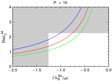
In order to be prepared for the improvement of the LHC bounds in question we define

[\Delta_{R}^{qq}(Z^{\prime})]_{\text{eff}}=\Delta_{R}^{qq}(Z^{\prime})\left[\frac{3\,{\rm TeV}}{M_{Z^{\prime}}}\right]^{2}.

(91)

In four panels in Fig. 1, corresponding to four values of $P$ indicated in each of them, we plot $|[\Delta_{R}^{qq}(Z^{\prime})]_{\text{eff}}|$ as a function of ${\rm Re}\Delta_{L}^{sd}(Z^{\prime})$ for different values of $B_{6}^{(1/2)}$ . For $M_{G^{\prime}}=M_{Z^{\prime}}$ the corresponding plot for $G^{\prime}$ can be obtained from Fig. 1 by either rescaling upwards all values of $P$ by a factor of $1.4$ or scaling down either $|[\Delta_{R}^{qq}(Z^{\prime})]_{\text{eff}}|$ or ${\rm Re}\Delta_{L}^{sd}(Z^{\prime})$ by the same factor. We will show such a plot in Section 6.4.

As we will discuss in Section 5.2 the values in the gray area corresponding to $|[\Delta_{R}^{qq}(Z^{\prime})]_{\text{eff}}|\geq 1.25$ and $|\Delta_{L}^{sd}(Z^{\prime})|\geq 2.3$ are basically ruled out by the LHC⁴⁴ 4 As mentioned in Section 5.2 the complete exclusion of the grey area would require more intensive study of points corresponding to larger values of $\Delta_{R}(Z^{\prime})$ and $M_{Z^{\prime}}<3\,{\rm TeV}$ .. We also note that while for $P=5$ and $P=10$ and $B_{6}^{(1/2)}\geq 1.0$ , the required values of ${\rm Re}\Delta_{L}^{sd}(Z^{\prime})$ are in the ballpark of unity, for $P=20$ they are generally larger than two implying for ${\rm Re}\Delta_{L}^{sd}(Z^{\prime})=2.3$

\alpha_{L}=\frac{[{\rm Re}\Delta_{L}^{sd}(Z^{\prime})]^{2}}{4\pi}=0.42~.

(92)

As $\alpha_{L}$ is not small let us remark that in in the case of a $U(1)$ gauge symmetry for even larger values of $\alpha_{L}$ it is difficult to avoid a Landau pole at higher scales. However, if only the coupling $\Delta_{L}^{sd}(Z^{\prime})$ is large, a simple renormalization group analysis shows that these scales are much larger than the LHC scales. Moreover, if $Z^{\prime}$ is associated with a non-abelian gauge symmetry that is asymptotically free ${\rm Re}\Delta_{L}^{sd}(Z^{\prime})$ could be even higher allowing to reach values of $P$ as high as $25-30$ . We will see in Section 6.4 that this is in fact the case for $G^{\prime}$ .

In this context a rough estimate of the perturbativity upper bound on $\Delta_{L}^{sd}(Z^{\prime})$ can be made by considering the loop expansion parameter⁵⁵ 5 A.J.B would like to thank Bogdan Dobrescu, Maikel de Vries and Andreas Weiler for discussions on this issue.

L=N\frac{[\Delta_{L}^{sd}(Z^{\prime})]^{2}}{16\pi^{2}}

(93)

where $N=3$ is the number of colours. For $\Delta_{L}^{sd}(Z^{\prime})=2.5,~3.0,~3.5$ one has $L=0.12,~0.17,~0.23$ , respectively, implying that using $\Delta_{L}^{sd}(Z^{\prime})$ as large as $2.3$ can certainly be defended.

Refer to caption — Figure 1: ${\rm Re}\Delta_{L}^{sd}(Z^{\prime})$ versus $|[\Delta_{R}^{qq}(Z^{\prime})]_{\text{eff}}|$ for $P=5,~10,~15,~20$ and $B_{6}^{(1/2)}=0.75$ (blue), $1.00$ (red) and $1.25$ (green). The gray area is basically excluded by the LHC. See Section 5.2.

4.5 Strategy

This discussion and an independent numerical analysis using the general formulae presented above leads us to the conclusion that for the goals of the present paper it is sufficient to consider only the following two scenarios for $Z^{\prime}$ couplings that satisfy the hierarchy (7):

Scenario A

This scenario is represented by our toy model constructed above. It provides significant contribution to the $\Delta I=1/2$ rule without violating constraints from $\Delta F=2$ processes. Here in addition to $\Delta_{L}^{sd}(Z^{\prime})$ and $\Delta_{R}^{qq}(Z^{\prime})$ of $\mathcal{O}(1)$ also a small $\Delta_{R}^{sd}(Z^{\prime})$ satisfying (84) is required. Undoubtedly this scenario is fine-tuned but cannot be excluded at present. Moreover, it implies certain correlations between various observables and it is interesting to investigate them numerically. The three steps procedure outlined above allows to study transparently this scenario.

Scenario B

Among flavour violating couplings only $\Delta_{L}^{sd}(Z^{\prime})$ is non-vanishing or at all relevant. In this case only SM operator contributes to $\varepsilon_{K}$ and $\Delta M_{K}$ and we deal with scenario LHS for flavour violating couplings not allowing for the necessary shift in $\rm{Re}A_{0}$ due to $\Delta M_{K}$ constraint but still providing interesting results for $\varepsilon^{\prime}/\varepsilon$ . Indeed only QCD penguin operator $Q_{6}$ contributes as in Scenario A to the NP part in $K_{L}\to\pi\pi$ in an important manner. But $\rm{Re}A_{0}^{\rm NP}$ in this scenario is very small and there is no relevant correlation between $\Delta I=1/2$ rule and remaining observables. The novel part of our analysis in this scenario relative to our previous papers is the analysis of $\varepsilon^{\prime}/\varepsilon$ and of its correlation with $K^{+}\rightarrow\pi^{+}\nu\bar{\nu}$ and $K_{L}\rightarrow\pi^{0}\nu\bar{\nu}$ .

5 Numerical Analysis

5.1 Preliminaries

In order to proceed we have to describe how we treat parametric and hadronic uncertainties in the SM contributions as this will determine the room left for NP contributions in the observables discussed by us.

First in order to simplify the numerical analysis we will set all parameters in Table 2, except for $|V_{ub}|$ and $|V_{cb}|$ , at their central values. Concerning the latter two we will investigate six scenarios for them in order to stress the importance of their determination in the context of the search for NP through various observables. In order to bound the parameters of the model and to take hadronic and parametric uncertainties into account we will first only require that in Scenario B the results for $\Delta M_{K}$ and $\varepsilon_{K}$ including NP contributions satisfy

0.75\leq\frac{\Delta M_{K}}{(\Delta M_{K})_{\rm SM}}\leq 1.25,\hskip 22.99988pt2.0\times 10^{-3}\leq|\varepsilon_{K}|\leq 2.5\times 10^{-3}.

(94)

However, it will be interesting to see what happens when the allowed range for $\varepsilon_{K}$ is reduced to $3\sigma$ range around its experimental value. In Scenario A which is easier numerically we will see more explicitly what happens to $\Delta M_{K}$ and $\varepsilon_{K}$ and the latter $3\sigma$ range will be more relevant than the use of (94).

We will set $M_{Z^{\prime}}=3~\,{\rm TeV}$ as our nominal value. This is an appropriate value for being consistent with ATLAS and CMS experiments although as we will discuss below such a mass puts an upper bound on $\Delta_{R}^{qq}(Z^{\prime})$ . The scaling laws in [33] and our discussion in Section 4.4 allow us to translate our results to other values of $M_{Z^{\prime}}$ . In particular when $\Delta_{L}^{sd}(Z^{\prime})$ is bounded by $\Delta S=2$ observables, NP effects in $\Delta F=1$ decrease with increasing $M_{Z^{\prime}}$ . Therefore in order that NP plays a role in the $\Delta I=1/2$ rule and the involved couplings are in perturbative regime, $M_{Z^{\prime}}$ should be smaller than $5~\,{\rm TeV}$ and consequently in the reach of the upgraded LHC.

Concerning the values of $\Delta_{L}^{sd}(Z^{\prime})$ the numerical analyses in Scenarios A and B differ in the following manner from each other:

•

In Scenario A, in which ${\rm Re}A_{0}$ plays an important role, we will use the three step procedure outlined in the previous section. In this manner we will find that $\Delta_{L}^{sd}(Z^{\prime})\geq 1$ in order for $Z^{\prime}$ to play any role in the $\Delta I=1/2$ rule.
•

In Scenario B, we can proceed as in our previous papers by using the parametrization

$\Delta_{L}^{sd}(Z^{\prime})=-\tilde{s}_{12}e^{-i\delta_{12}},$ (95)

and searching for the allowed oases in the space $(\tilde{s}_{12},\delta_{12})$ that satisfy the constraints in (94) or the stronger $3\sigma$ constraint for $\varepsilon_{K}$ . In this scenario $\Delta_{L}^{sd}(Z^{\prime})$ will turn out to be very small. We will not show the results for these oases as they can be found in [26].

Having determined $\Delta_{L}^{sd}(Z^{\prime})$ we can proceed to calculate the $\Delta F=1$ observables and study correlations between them. Here additional uncertainties will come from $B_{6}^{(1/2)}$ which is hidden in the condition (47) so that it does not appear explicitly in NP contributions but affects the SM contribution to $\varepsilon^{\prime}/\varepsilon$ . Also $Z^{\prime}$ coupling to neutrinos has to be fixed.

$G_{F}=1.16637(1)\times 10^{-5}\,{\rm GeV}^{-2}$ [1]	$M_{W}=80.385(15)\,{\rm GeV}$ [1]
$\sin^{2}\theta_{W}=0.23116(13)$ [1]	$\alpha(M_{Z})=1/127.9$ [1]
$\alpha_{s}(M_{Z})=0.1185(6)$ [1]	$m_{K}=497.614(24)\,{\rm MeV}$ [65]
$m_{u}(2\,{\rm GeV})=(2.1\pm 0.1)\,{\rm MeV}$ [50]	$m_{\pi}=135.0\,{\rm MeV}$
$m_{d}(2\,{\rm GeV})=(4.68\pm 0.16)\,{\rm MeV}$ [50]	$F_{\pi}=129.8\,{\rm MeV}$
$m_{s}(2\,{\rm GeV})=(93.8\pm 2.4)\,{\rm MeV}$ [50]	$F_{K}=156.1(11)\,{\rm MeV}$ [66]
$m_{c}(m_{c})=(1.279\pm 0.013)\,{\rm GeV}$ [67]	$\|V_{us}\|=0.2252(9)$ [68]
$m_{b}(m_{b})=4.19^{+0.18}_{-0.06}\,{\rm GeV}$ [1]	$\|V^{\text{incl.}}_{ub}\|=(4.41\pm 0.31)\times 10^{-3}$ [1]
$m_{t}(m_{t})=163(1)\,{\rm GeV}$ [66, 69]	$\|V^{\text{excl.}}_{ub}\|=(3.23\pm 0.31)\times 10^{-3}$ [1]
$\eta_{cc}=1.87(76)$ [70]	$\|V_{cb}\|=(40.9\pm 1.1)\times 10^{-3}$ [1]
$\eta_{tt}=0.5765(65)$ [71]	$\hat{B}_{K}=0.75$
$\eta_{ct}=0.496(47)$ [72]	$\kappa_{\epsilon}=0.94(2)$ [63, 64]

Table 2: Values of the experimental and theoretical quantities used as input parameters.

Finally uncertainties due to the values of the CKM elements $|V_{cb}|$ and $|V_{ub}|$ have to be considered. These uncertainties are at first sight absent in $Z^{\prime}$ contributions but affect the SM predictions for $\varepsilon_{K}$ and $\varepsilon^{\prime}/\varepsilon$ and consequently indirectly also $Z^{\prime}$ contributions through the size of allowed range for $\Delta^{sd}_{L}(Z^{\prime})$ in both scenarios A and B. Indeed $\varepsilon^{\prime}/\varepsilon$ and $K_{L}\rightarrow\pi^{0}\nu\bar{\nu}$ depend in the SM on ${\rm{Im}\lambda_{t}}$ , while $\varepsilon_{K}$ and $K^{+}\rightarrow\pi^{+}\nu\bar{\nu}$ on both ${\rm{Im}\lambda_{t}}$ and ${\rm{Re}\lambda_{t}}$ . Now within the accuracy of better than $0.5\%$

{\rm{Im}\lambda_{t}}=|V_{ub}||V_{cb}|\sin\gamma,\hskip 22.99988pt{\rm{Re}\lambda_{t}}=-{\rm{Im}\lambda_{t}}\cot(\beta-\beta_{s})

(96)

with $\gamma$ and $\beta$ being the known angles of the unitarity triangle and $-\beta_{s}\approx 1^{\circ}$ is the phase of $V_{ts}$ after the minus sign has been factored out. Consequently, within the SM not only $\varepsilon^{\prime}/\varepsilon$ and $\varepsilon_{K}$ but also the branching ratios for $K^{+}\rightarrow\pi^{+}\nu\bar{\nu}$ and $K_{L}\rightarrow\pi^{0}\nu\bar{\nu}$ will depend sensitively on the chosen values for $|V_{cb}|$ and $|V_{ub}|$ .

One should recall that the typical values for $|V_{ub}|$ and $|V_{cb}|$ extracted from inclusive decays are (see [73, 74] and refs therein)⁶⁶ 6 We prefer to quote for the central value of $|V_{cb}|$ the most recent value from [74] than the one given in Table 2.

|V_{ub}|=4.1\times 10^{-3},\hskip 22.99988pt|V_{cb}|=42.0\times 10^{-3}

(97)

while the typical values extracted from exclusive decays read [75, 76]

|V_{ub}|=3.2\times 10^{-3},\hskip 22.99988pt|V_{cb}|=39.0\times 10^{-3}.

(98)

As the determinations of $|V_{ub}|$ and $|V_{cb}|$ are independent of each other it will be instructive to consider the following scenarios for these elements:

$\displaystyle a)$	$\displaystyle\hskip 22.99988pt\|V_{ub}\|=3.2\times 10^{-3}\hskip 22.99988pt\|V_{cb}\|=39.0\times 10^{-3}\hskip 22.99988pt({\rm purple)}$	(99)
$\displaystyle b)$	$\displaystyle\hskip 22.99988pt\|V_{ub}\|=3.2\times 10^{-3}\hskip 22.99988pt\|V_{cb}\|=42.0\times 10^{-3}\hskip 22.99988pt({\rm cyan)}$	(100)
$\displaystyle c)$	$\displaystyle\hskip 22.99988pt\|V_{ub}\|=4.1\times 10^{-3}\hskip 22.99988pt\|V_{cb}\|=39.0\times 10^{-3}\hskip 22.99988pt({\rm magenta)}$	(101)
$\displaystyle d)$	$\displaystyle\hskip 22.99988pt\|V_{ub}\|=4.1\times 10^{-3}\hskip 22.99988pt\|V_{cb}\|=42.0\times 10^{-3}\hskip 22.99988pt({\rm yellow)}$	(102)
$\displaystyle e)$	$\displaystyle\hskip 22.99988pt\|V_{ub}\|=3.7\times 10^{-3}\hskip 22.99988pt\|V_{cb}\|=40.5\times 10^{-3}\hskip 22.99988pt({\rm green)}$	(103)
$\displaystyle f)$	$\displaystyle\hskip 22.99988pt\|V_{ub}\|=3.9\times 10^{-3}\hskip 22.99988pt\|V_{cb}\|=42.0\times 10^{-3}\hskip 22.99988pt({\rm blue)}$	(104)

where we also included two additional scenarios, one for averaged values of $|V_{ub}|$ and $|V_{cb}|$ and the last one ( $f)$ ) particularly suited for the analysis of Scenario A. We also give the colour coding for these scenarios used in the plots.

Concerning the parameter $\hat{B}_{K}$ which enters the evaluation of $\varepsilon_{K}$ the world average from lattice QCD is $\hat{B}_{K}=0.766\pm 0.010$ [50], very close to the strictly large $N$ limit value $\hat{B}_{K}=0.75$ . On the other hand the recent calculation within the dual approach to QCD gives $\hat{B}_{K}=0.73\pm 0.02$ [17]. Moreover, the analysis in [77] indicates that in the absence of significant $1/N^{2}$ corrections to the leading large $N$ value one should have $\hat{B}_{K}\leq 0.75$ . It is an interesting question whether this result will be confirmed by future lattice calculations which have a better control over the uncertainties than it is possible within the approach in [17, 77]. For the time being it is a very good approximation to set simply $\hat{B}_{K}=0.75$ . Indeed compared to the present uncertainties from $|V_{cb}|$ and $|V_{ub}|$ in $\varepsilon_{K}$ proceeding in this manner is fully justified.

Concerning the value of $\gamma$ we will just set $\gamma=68^{\circ}$ . This is close to central values from recent determinations [78, 79, 80] and varying $\gamma$ simultaneously with $|V_{cb}|$ and $|V_{ub}|$ would not improve our analysis.

As seen in Table 3 the six scenarios for CKM parameters imply rather different values of ${\rm{Im}\lambda_{t}}$ and ${\rm{Re}\lambda_{t}}$ and consequently different values for various observables considered by us. This is seen in this table where we give SM values for $\varepsilon_{K}$ , $\Delta M_{K}$ , $\Delta M_{s}$ , $\Delta M_{d}$ , $S_{\psi K_{S}}$ , $\varepsilon^{\prime}/\varepsilon$ , $\mathcal{B}(K_{L}\rightarrow\pi^{0}\nu\bar{\nu})$ and $\mathcal{B}(K^{+}\rightarrow\pi^{+}\nu\bar{\nu})$ together with their experimental values. To this end we have used the central values of the remaining parameters, relevant for $B_{s,d}^{0}$ systems collected in [61]. For completeness we give also the values for $\overline{\mathcal{B}}(B_{s}\to\mu^{+}\mu^{-})$ and ${\mathcal{B}}(B_{d}\to\mu^{+}\mu^{-})$ .

We would like to warn the reader that the SM values for various observables in Table 3 have been obtained directly by using CKM parameters from tree-level decays and consequently differ from SM results obtained usually from Unitarity Triangle fits that include constraints from processes in principle affected by NP.

We note that for a given choice of $|V_{ub}|$ , $|V_{cb}|$ and $\gamma$ the SM predictions can differ sizably from the data but these departures are different for different scenarios:

•

Only in scenario $a)$ does $S_{\psi K_{S}}^{\rm SM}$ agree fully with the data. On the other hand in the remaining scenarios $Z^{\prime}$ contributions to $B_{d}^{0}-\bar{B}_{d}^{0}$ are required to bring the theory to agree with the data. But then also $\Delta M_{s}$ and $\Delta M_{d}$ have to receive new contributions, even in the case of scenario $a)$ . As in the models considered here $Z^{\prime}$ flavour violating couplings involving $b$ -quarks are not fixed, this can certainly be achieved. We refer to [26, 32] for details.
•

On the other hand $\varepsilon_{K}$ is definitely below the experimental value in scenario $a)$ but roughly consistent with experiment in other scenarios leaving still some room for NP contributions. In particular in scenarios $d)$ and $f)$ it is close to its experimental value.
•

$\Delta M_{K}$ is as expected the same in all scenarios and roughly $10\%$ below its experimental value. But we should remember that the large uncertainty in $\eta_{cc}$ corresponds to $\pm 40\%$ uncertainty in $\Delta M_{K}$ and still sizable NP contributions are allowed.
•

The dependence of $\mathcal{B}(K_{L}\rightarrow\pi^{0}\nu\bar{\nu})$ on scenario considered is large but moderate in the case of $\mathcal{B}(K^{+}\rightarrow\pi^{+}\nu\bar{\nu})$ .
•

We emphasize strong dependence on $|V_{cb}|$ and consequently on $|V_{ts}|$ of the branching ratios $\overline{\mathcal{B}}(B_{s}\to\mu^{+}\mu^{-})$ and ${\mathcal{B}}(B_{d}\to\mu^{+}\mu^{-})$ . For exclusive values of $|V_{cb}|$ both branching ratios are significantly lower than the official SM values [81] obtained using $|V_{cb}|=42.4\times 10^{-3}$ .

In Scenario B, where the constraint from $\Delta I=1/2$ is absent we will have more freedom in adjusting NP parameters to improve in each of the scenarios $a)-f)$ the agreement of the theory with data but within Scenario A we will find that only for certain scenarios of CKM parameters it will be possible to fit the data.

In Fig. 2 we summarize those results of Table 3 that will help us in following our numerical analysis in various NP scenarios presented by us. In particular we observe in the lower left panel strong correlation between $\varepsilon^{\prime}/\varepsilon$ and $\mathcal{B}(K_{L}\rightarrow\pi^{0}\nu\bar{\nu})$ . Fig. 2 shows graphically how important the determination of $|V_{ub}|$ , $|V_{cb}|$ and $B_{6}^{(1/2)}$ in the indirect search for NP is. Let us hope that at the end of this decade there will be only a single point representing the SM in each of these four panels.

	$a)$	$b)$	$c)$	$d)$	$e)$	$f)$	Data
$\rm{Im}\lambda_{t}\,[10^{-4}]$	$1.16$	$1.25$	$1.48$	$1.60$	$1.39$	$1.52$	$-$
$\rm{Re}\lambda_{t}\,[10^{-4}]$	$-2.90$	$-3.40$	$-2.76$	$-3.25$	$-3.07$	$-3.29$	$-$
$S^{\rm SM}_{\psi K_{S}}$	$0.664$	$0.622$	$0.808$	$0.765$	$0.726$	$0.736$	$0.679(20)$
$\Delta M_{s}\,[\text{ps}^{-1}]$	$15.92$	$18.44$	$15.99$	$18.51$	$17.19$	$18.49$	$17.69(8)$
$\Delta M_{d}\,[\text{ps}^{-1}]$	$0.47$	$0.54$	$0.47$	$0.54$	$0.50$	$0.54$	$0.510(4)$
$\Delta M_{K}\,[10^{-3}\text{ps}^{-1}]$	$4.70$	$4.72$	$4.70$	$4.71$	$4.71$	$4.72$	$5.293(9)$
$\|\varepsilon_{K}\|\,[10^{-3}]$	$1.56$	$1.89$	$1.93$	$2.35$	$1.96$	$2.25$	$2.228(11)$
$\varepsilon^{\prime}/\varepsilon\,[10^{-4}](B_{6}^{(1/2)}=0.75)$	$8.0$	$8.6$	$10.2$	$11.0$	$9.6$	$10.5$	$16.5\pm 2.6$
$\varepsilon^{\prime}/\varepsilon\,[10^{-4}](B_{6}^{(1/2)}=1.00)$	$12.9$	$13.9$	$16.5$	$17.8$	$15.5$	$16.9$	$16.5\pm 2.6$
$\varepsilon^{\prime}/\varepsilon\,[10^{-4}](B_{6}^{(1/2)}=1.25)$	$17.8$	$19.2$	$22.8$	$24.6$	$21.4$	$23.4$	$16.5\pm 2.6$
$\mathcal{B}(K_{L}\to\pi^{0}\nu\bar{\nu})\,[10^{-11}]$	$2.01$	$2.33$	$3.29$	$3.82$	$2.89$	$3.45$	$\leq 2.6\cdot 10^{-8}$
$\mathcal{B}(K^{+}\to\pi^{+}\nu\bar{\nu})\,[10^{-11}]$	$7.65$	$9.40$	$7.54$	$9.25$	$8.40$	$9.28$	$17.3^{+11.5}_{-10.5}$
$\overline{\mathcal{B}}(B_{s}\to\mu^{+}\mu^{-})\,[10^{-9}]$	$3.00$	$3.47$	$3.01$	$3.48$	$3.23$	$3.48$	$2.9\pm 0.7$
$\mathcal{B}(B_{d}\to\mu^{+}\mu^{-})\,[10^{-10}]$	$0.94$	$1.09$	$0.94$	$1.09$	$1.01$	$1.09$	$3.6^{+1.6}_{-1.4}$

Table 3: Values of

\rm{Im}\lambda_{t}

\rm{Re}\lambda_{t}

and of several observables within the SM for various scenarios of CKM elements as discussed in the text.

5.2 LHC Constraints

Finally, we should remember that $Z^{\prime}$ couplings to quarks can be bounded by collider data as obtained from LEP-II and the LHC. In the case of LEP-II all the bounds can be satisfied in our models by using sufficiently small leptonic couplings. However, in the case of $\Delta_{R}^{qq}$ and $\Delta_{L}^{sd}$ we have to check whether the values $\Delta_{R}^{qq}(Z^{\prime})=\mathcal{O}(1)$ and $\Delta_{L}^{sd}(Z^{\prime})=\mathcal{O}(1)$ necessary for a significant $Z^{\prime}$ contribution to ${\rm Re}A_{0}$ are allowed by the ATLAS and CMS outcome of the search for narrow resonances using dijet mass spectrum in proton-proton collisions and by the effective operator bounds.

Bounds of this sort can be found in [87, 88, 89, 90, 40] but the $Z^{\prime}$ models considered there have SM couplings or as in the case of [40] all diagonal couplings, both left-handed and right-handed, are flavour universal which is not the case of our models in which the hierarchy (7) is assumed.

For this reason a dedicated analysis of our toy model has been performed [82]⁷⁷ 7 The details of this analysis will be presented elsewhere. using the most recent results from ATLAS and CMS. The result of this study is presented in Fig. 3 and can be briefly summarized as follows:

•

The most up to date dijet searches from ATLAS [85] and CMS [86] allow to put an upper bound on $|\Delta_{R}^{qq}(Z^{\prime})|$ but only for $|\Delta_{R}^{qq}(Z^{\prime})|\leq 0.8$ . As seen in Fig. 3 this maximal value is only allowed for $M_{Z^{\prime}}\geq 2.4\,{\rm TeV}$ .
•

A second source of exclusion limits for $Z^{\prime}$ boson couplings comes from effective operator limits, in this case from four-quark operators studied by both ATLAS [83] and CMS [84]. As seen in Fig. 3 the upper bound on $|\Delta_{R}^{qq}(Z^{\prime})|$ can be summarized by

$|\Delta_{R}^{qq}(Z^{\prime})|\leq 1.0\times\left[\frac{M_{Z^{\prime}}}{3\,{\rm TeV}}\right].$ (105)

The following additional comments should be made in connection with results in Fig. 3:

•

The dijet limits are only effective if the width of the $Z^{\prime}$ or $G^{\prime}$ is below $15\%$ for ATLAS and $10\%$ for CMS.
•

The lack of exclusion limits for CMS around $M_{Z^{\prime}}=3.5$ TeV are the result of a fluctuation in the data and therefore their exclusion limits.
•

It is important to note that the limits from effective operator constraints should not to be trusted when the center of mass energy of the experiment is bigger than the mass of the particle which is integrated out. For this analysis the effective center of mass energy is $3\,{\rm TeV}$ .

While dijets constraints would still allow for $[\Delta_{R}^{qq}(Z^{\prime})]_{\text{eff}}=1.25$ (see (91)) we will use for it $1.0$ so that our nominal values will be

\Delta_{R}^{qq}(Z^{\prime})=-1.0,\hskip 22.99988ptM_{Z^{\prime}}=3\,{\rm TeV}

(106)

that is consistent with the bound in (105). As seen in (47) the couplings $\Delta_{R}^{qq}(Z^{\prime})$ and $\Delta_{L}^{sd}(Z^{\prime})$ must have opposite signs in order to satisfy the $\Delta I=1/2$ constraint. On the basis of the present LHC data it is not possible to decide which of the two possible sign choices for these couplings is favoured by the collider data but this could be in principle possible in the future. The minus in $\Delta_{R}^{qq}(Z^{\prime})$ is chosen here only to keep the coupling $\Delta_{L}^{sd}(Z^{\prime})$ positive definite but presently the same results would be obtained with the other choice for signs of these two couplings.

As far as $\Delta_{L}^{sd}(Z^{\prime})$ is concerned the derivation of corresponding bounds is more difficult, since the experimental collaborations do not provide constraints for flavoured four quark interactions. However, there have been efforts to obtain these from the current data [88, 91]. In particular the analysis of the $\Delta S=2$ operator in [91] turns out to be useful. With its help one finds the upper bound [82]

|\Delta_{L}^{sd}(Z^{\prime})|\leq 2.3\left[\frac{M_{Z^{\prime}}}{3\,{\rm TeV}}\right].

(107)

Now, as seen in Fig. 1 with (106) the values $P=20-30$ require ${\rm Re}\Delta_{L}^{sd}(Z^{\prime})\approx 3-4$ dependently on the value of $B_{6}^{(1/2)}$ . This would still be consistent with rough perturbativity bound ${\rm Re}\Delta_{L}^{sd}(Z^{\prime})\leq 4$ discussed by us in Section 4.4. However, the LHC bound in (107), seems to exclude this possibility, although a dedicated analysis of this bound including simultaneously left-handed and right-handed couplings would be required to put this bound on a firm footing. We hope to return to such an analysis in the future. For the time being we conclude that the maximal values of $P$ possible in this NP scenario are in the ballpark of $16$ , that is roughly of the size of SM QCD penguin contribution.

Indeed, combining the bounds on the couplings of $Z^{\prime}$ and its mass and using the relation (47) we arrive at the upper bound

P\leq 16\left[\frac{B_{6}^{(1/2)}}{1.0}\right],\hskip 22.99988pt(Z^{\prime})~.

(108)

This result is also seen in Fig. 1. In principle for $B_{6}^{(1/2)}$ significantly larger than unity one could increase the value of $P$ above 20 but as we will see soon this is not allowed when simultaneously the correlation between $\varepsilon^{\prime}/\varepsilon$ and $\varepsilon_{K}$ is taken into account.

At this point it should be emphasized that the dashed surface in Fig. 3 has in fact not been completely excluded by ATLAS and CMS analyses and as an example $\Delta_{R}^{qq}(Z^{\prime})=-1.5$ and $M_{Z^{\prime}}=2.5\,{\rm TeV}$ , allowing $P$ as high as $30$ , is still a valid point. While it is likely that a dedicated analysis of this model by ATLAS and CMS in this range of parameters would exclude the dashed surface completely, such an analysis has still to be done.

5.3 Results

5.3.1 SM Results for $\varepsilon^{\prime}/\varepsilon$

We begin our presentation by discussing briefly the SM prediction for $\varepsilon^{\prime}/\varepsilon$ given in Table 3 for different scenarios for CKM couplings and three values of $B_{6}^{(1/2)}$ . We observe that for $B_{6}^{(1/2)}=1.00$ , except for scenario $a)$ , the SM is in good agreement with the data but in view of the experimental error NP at the level of $\pm 20\%$ can still contribute. In the past when $B_{8}^{(3/2)}=1.0$ was used $\varepsilon^{\prime}/\varepsilon$ for $B_{6}^{(1/2)}=1.0$ was below the data, but with the lattice result $B_{8}^{(3/2)}=0.65\pm 0.05$ [21] it looks like $B_{6}^{(1/2)}\approx 1.0$ is the favourite value within the SM. Except for scenario $a)$ and $B_{6}^{(1/2)}=1.25$ for which SM gives values consistent with experiment, for other two values of $B_{6}^{(1/2)}$ we get either visibly lower or visibly higher values of $\varepsilon^{\prime}/\varepsilon$ than measured and some NP is required to fit the data.

5.4 Scenario A

The question then arises whether simultaneous agreement with the data for ${\rm{Re}}A_{0}$ , $\varepsilon_{K}$ and $\varepsilon^{\prime}/\varepsilon$ can be obtained in the toy $Z^{\prime}$ model introduced by us.

We use the three step procedure suited for this scenario that we outlined in the previous section. Investigating all six scenarios $a)-f)$ for $(|V_{cb}|,|V_{ub}|)$ we have found that only in scenarios $d)$ and $f)$ it is possible to obtain satisfactory agreement with the data on $\varepsilon^{\prime}/\varepsilon$ and $\varepsilon_{K}$ for significant values of $P$ . Indeed due to relation (90) NP in $\varepsilon_{K}$ must be small in order to keep $\varepsilon^{\prime}/\varepsilon$ under control. As seen in Fig. 2 this is only the case in these two CKM scenarios. Yet, as seen in Fig. 4, even $d)$ and $f)$ scenarios can be distinguished by the correlation between $\varepsilon^{\prime}/\varepsilon$ and $\varepsilon_{K}$ demonstrating again how important it is to determine precisely $|V_{cb}|$ and $|V_{ub}|$ .

While, as seen in (90), the correlation between NP contributions to $\varepsilon^{\prime}/\varepsilon$ and $\varepsilon_{K}$ depends at fixed $r_{\Delta M}$ only on $P$ , in the case of SM contributions it depends explicitly on $B_{6}^{(1/2)}$ . Therefore we show in Fig. 4 the lines for $B_{6}^{(1/2)}=0.75,~1.00,~1.25$ using the colour coding

B_{6}^{(1/2)}=0.75~\text{(blue)},\hskip 11.49994ptB_{6}^{(1/2)}=1.0~\text{(red)},\hskip 11.49994ptB_{6}^{(1/2)}=1.25~\text{(green)}.

(109)

The three lines carrying the same colour correspond to four values of $P=5,~10,~15,~20$ . With increasing $P$ the lines become steeper. The dark(light) gray region corresponds to the $1(2)\sigma$ experimental range for $\varepsilon^{\prime}/\varepsilon$ and $3\sigma$ range for $\varepsilon_{K}$ .

Beginning with scenario $d)$ We observe that only the following combinations of $P$ and $B_{6}^{(1/2)}$ are consistent with this range:

•

For $B_{6}^{(1/2)}=1.25$ only $P=5,~10,~15$ are allowed when $1\sigma$ range for $\varepsilon^{\prime}/\varepsilon$ is considered. At $2\sigma$ also $P=20$ is allowed. Larger values of $P$ are only possible for $B_{6}^{(1/2)}>1.25$ . We conclude therefore that for $B_{6}^{(1/2)}=1.25$ we find the upper bound $P\leq 20$ .
•

For $B_{6}^{(1/2)}=1.00$ the corresponding upper bound amounts to $P\leq 10$ .
•

For $B_{6}^{(1/2)}=0.75$ even for $P=5$ one cannot obtain simultaneous agreement with the data on $\varepsilon^{\prime}/\varepsilon$ and $\varepsilon_{K}$ .

A rather different pattern is found for scenario $f)$ :

•

For $B_{6}^{(1/2)}=1.25$ the values $P=5,~10,~15,~20$ are not allowed even at $2\sigma$ range for $\varepsilon^{\prime}/\varepsilon$ but decreasing slightly $B_{6}^{(1/2)}$ would allow values $P\geq 20$ .
•

On the other hand, in the case of $B_{6}^{(1/2)}=1.00$ there is basically no restriction on $P$ from this correlation simply because in this scenario NP contributions to $\epsilon_{K}$ are small (see Fig. 2). In fact in this case values of $P$ as high as $30$ would be allowed. While such values are not possible in the case of $Z^{\prime}$ due to LHC constraint in (108) we will see that they are allowed in the case of $G^{\prime}$ .
•

Similar situation is found for $B_{6}^{(1/2)}=0.75$ although here at $1\sigma$ for $\varepsilon^{\prime}/\varepsilon$ one finds the bound $P\geq 10$ .

We conclude therefore that in view of the fact that NP effects in $\varepsilon^{\prime}/\varepsilon$ in our toy model are by an order of magnitude larger than in $\varepsilon_{K}$ , scenario $f)$ is particularly suited for allowing large values of $P$ as it avoids strong constraints from $\varepsilon^{\prime}/\varepsilon$ and $\varepsilon_{K}$ . In scenario $d)$ independently of the LHC we find $P<20$ . While in the case of $Z^{\prime}$ model at hand this virtue of scenario $f)$ cannot be fully used because of the LHC constraint (108) we will see in the next section that it plays a role in the case of $G^{\prime}$ model. These findings are interesting as they imply that only for the inclusive determinations of $|V_{ub}|$ and $|V_{cb}|$ $Z^{\prime}$ has a chance to contribute in a significant manner to the $\Delta I=1/2$ rule. This assumes the absence of other mechanisms at work which otherwise could help in this case if the exclusive determinations of these CKM parameters would turn out to be true.

In Fig. 5 we show with darker colours the allowed values of ${\rm Re}\Delta_{L}^{sd}$ and ${\rm Im}\Delta_{L}^{sd}$ in scenario A for CKM values $d)$ and $f)$ that correspond to the values of $P$ and $B_{6}^{(1/2)}$ selected by the light gray region in Fig. 4. In lighter colours we show the allowed values of ${\rm Re}\Delta_{L}^{sd}$ and ${\rm Im}\Delta_{L}^{sd}$ using (94) as constraint for $\varepsilon_{K}$ . As for $M_{Z^{\prime}}=3\,{\rm TeV}$ only values $|\Delta_{R}^{qq}|\leq 1.0$ are allowed by the LHC bound in (105), the green and yellow ranges are ruled out but we show them anyway as this demonstrates the power of the LHC in constraining our model. Among the remaining areas the red one is favoured as it corresponds to smaller values of ${\rm Re}\Delta_{L}^{sd}$ for a given $P$ and this is the reason why $\Delta_{R}^{qq}=-1.0$ has been chosen as nominal value for this coupling. This feature is not clearly seen in this figure where we varied $P$ but this is evident from plots in Fig. 1. The vertical black line shows the LHC bound in (107). Only values on the left of this line are allowed.

We have investigated the correlation between $\mathcal{B}(K_{L}\rightarrow\pi^{0}\nu\bar{\nu})$ and $\mathcal{B}(K^{+}\rightarrow\pi^{+}\nu\bar{\nu})$ for scenarios $d)$ and $f)$ finding the following pattern that follows from the fact that in Scenario A, as can be seen in Fig. 5, ${\rm Re}\Delta_{L}^{sd}(Z^{\prime})=\mathcal{O}(1)$ . In view of this, the neutrino coupling $\Delta_{L}^{\nu\nu}(Z^{\prime})$ must be sufficiently small in order to be consistent with the data on $\mathcal{B}(K^{+}\rightarrow\pi^{+}\nu\bar{\nu})$ . But as seen in Fig. 5 ${\rm Im}\Delta_{L}^{sd}(Z^{\prime})$ is required to be small in order to satisfy the data on $\varepsilon^{\prime}/\varepsilon$ and $\varepsilon_{K}$ . The smallness of both $\Delta_{L}^{\nu\nu}(Z^{\prime})$ and ${\rm Im}\Delta_{L}^{sd}(Z^{\prime})$ implies in this scenario negligible NP contributions to $\mathcal{B}(K_{L}\rightarrow\pi^{0}\nu\bar{\nu})$ . Thus the main message from this exercise is that $\mathcal{B}(K_{L}\rightarrow\pi^{0}\nu\bar{\nu})$ remains SM-like, while $\mathcal{B}(K^{+}\rightarrow\pi^{+}\nu\bar{\nu})$ can be modified but this modification depends on the size of the unknown coupling $\Delta_{L}^{\nu\nu}(Z^{\prime})$ and changing its sign one can obtain both suppression or enhancement of $\mathcal{B}(K^{+}\rightarrow\pi^{+}\nu\bar{\nu})$ relative to the SM value. For $\Delta_{L}^{\nu\nu}(Z^{\prime})$ in the ballpark of $5\times 10^{-4}$ significant enhancements or suppressions can be obtained. In view of this simple pattern and low predictive power we refrain from showing any plots.

Yet, the requirement of strongly suppressed leptonic couplings implies that unless $\Delta_{L,R}^{sb}(Z^{\prime})$ and $\Delta_{L,R}^{db}(Z^{\prime})$ are sizable, in Scenario A NP contributions to rare $B_{s,d}$ decays with neutrinos and charged leptons in the final state are predicted to be small. On the other hand these effects could be sufficiently large in $\Delta B=2$ processes to cure SM problems in scenarios $d$ and $f$ seen in Table 3.

While for a fixed value of $\Delta_{L}^{\nu\nu}(Z^{\prime})$ there exist correlations between $\varepsilon^{\prime}/\varepsilon$ and $\mathcal{B}(K^{+}\rightarrow\pi^{+}\nu\bar{\nu})$ such correlations are more interesting in the case of Scenario B which we will discuss next.

5.5 Scenario B

Here we proceed as in [26] except that we use scenarios $a)-f)$ for $(|V_{cb}|,|V_{ub}|)$ and also present results for $\varepsilon^{\prime}/\varepsilon$ . To this end we use colour coding for these scenarios in (99)-(104) and the one for $B_{6}^{(1/2)}$ in (109) and set

\Delta_{R}^{qq}(Z^{\prime})=0.5,\,1.0,\hskip 22.99988pt\Delta_{L}^{\nu\nu}(Z^{\prime})=0.5\,

(110)

with darker(lighter) colours representing $\Delta_{R}^{qq}(Z^{\prime})=1.0(0.5)$ . These values of $\Delta_{R}^{qq}(Z^{\prime})$ satisfy LHC bounds. The neutrino coupling can be chosen as in our previous papers because the coupling $\Delta_{L}^{sd}(Z^{\prime})$ will be bounded by $\Delta M_{K}$ and $\varepsilon_{K}$ to be very small and this choice is useful as it allows to see the impact of $\varepsilon^{\prime}/\varepsilon$ constraint on our results for rare decays $K^{+}\rightarrow\pi^{+}\nu\bar{\nu}$ and $K_{L}\rightarrow\pi^{0}\nu\bar{\nu}$ obtained in [26] without this constraint.

We find that due to the absence of the constraint from the $\Delta I=1/2$ rule in all six scenarios for $(|V_{cb}|,|V_{ub}|)$ agreement with the data on $\varepsilon_{K}$ and $\varepsilon^{\prime}/\varepsilon$ can be obtained. In Fig. 6 we show the correlation between $\mathcal{B}(K_{L}\rightarrow\pi^{0}\nu\bar{\nu})$ and $\mathcal{B}(K^{+}\rightarrow\pi^{+}\nu\bar{\nu})$ for the six scenarios $a)-f)$ for $(|V_{cb}|,|V_{ub}|)$ . In Figs. 7 and 8 we show correlations of $\varepsilon^{\prime}/\varepsilon$ with $\mathcal{B}(K_{L}\rightarrow\pi^{0}\nu\bar{\nu})$ and $\mathcal{B}(K^{+}\rightarrow\pi^{+}\nu\bar{\nu})$ , respectively.

We make the following observations:

•

The plot in Fig. 6 is familiar from other NP scenarios. $\mathcal{B}(K_{L}\rightarrow\pi^{0}\nu\bar{\nu})$ can be strongly enhanced on one of the branches and then $\mathcal{B}(K^{+}\rightarrow\pi^{+}\nu\bar{\nu})$ is also enhanced. But $\mathcal{B}(K^{+}\rightarrow\pi^{+}\nu\bar{\nu})$ can also be enhanced without modifying $\mathcal{B}(K_{L}\rightarrow\pi^{0}\nu\bar{\nu})$ . The last feature is not possible within the SM and any model with minimal flavour violation in which these two branching ratios are strongly correlated.
•

As seen in Fig. 7 except for the smallest values of $\mathcal{B}(K_{L}\rightarrow\pi^{0}\nu\bar{\nu})$ , where this branching ratio is below the SM predictions, in each scenario there is a strong correlation between $\varepsilon^{\prime}/\varepsilon$ and this branching ratio so that for fixed $B_{6}^{(1/2)}$ the increase of $\varepsilon^{\prime}/\varepsilon$ uniquely implies the increase of $\mathcal{B}(K_{L}\rightarrow\pi^{0}\nu\bar{\nu})$ . In this case as seen in Fig. 6 also $\mathcal{B}(K^{+}\rightarrow\pi^{+}\nu\bar{\nu})$ increases so that we have actually a triple correlation.
•

We note that even a small increase of $\varepsilon^{\prime}/\varepsilon$ for fixed values of $B_{6}^{(1/2)}$ implies a strong increase of $\mathcal{B}(K_{L}\rightarrow\pi^{0}\nu\bar{\nu})$ . But this hierarchy applies only for $\Delta_{R}^{qq}(Z^{\prime})$ and $\Delta_{L}^{\nu\nu}(Z^{\prime})$ being of the same order as assumed in (110). Introducing a hierarchy in these couplings would change the effects in favour of $\varepsilon^{\prime}/\varepsilon$ or $\mathcal{B}(K_{L}\rightarrow\pi^{0}\nu\bar{\nu})$ relative to the results presented by us. In the case of $Z$ boson with FCNCs analyzed in Section 7, where all diagonal couplings are fixed, definite results for this correlation will be obtained.
•

Values of $B_{6}^{(1/2)}=1.25$ are disfavored for scenarios $c)-f)$ unless $\mathcal{B}(K_{L}\rightarrow\pi^{0}\nu\bar{\nu})$ is suppressed with respect to the SM value.
•

For $B_{6}^{(1/2)}=1.0$ the branching ratio $\mathcal{B}(K_{L}\rightarrow\pi^{0}\nu\bar{\nu})$ can reach values as high as $10^{-10}$ but in view of the experimental error in $\varepsilon^{\prime}/\varepsilon$ this is not required by $\varepsilon^{\prime}/\varepsilon$ .
•

For $B_{6}^{(1/2)}=0.75$ SM prediction for $\varepsilon^{\prime}/\varepsilon$ is in all scenarios $a)-f)$ visibly below the data and curing this problem with $Z^{\prime}$ exchange enhances $\mathcal{B}(K_{L}\rightarrow\pi^{0}\nu\bar{\nu})$ typically above $1.5\times 10^{-10}$ .
•

The main message from these plots is that values of $\mathcal{B}(K_{L}\rightarrow\pi^{0}\nu\bar{\nu})$ as large as several $10^{-10}$ are not possible when $\varepsilon^{\prime}/\varepsilon$ constraint is taken into account unless the coupling $\Delta_{R}^{qq}(Z^{\prime})$ is chosen to be much smaller than assumed by us.
•

The correlation between $\varepsilon^{\prime}/\varepsilon$ and $\mathcal{B}(K^{+}\rightarrow\pi^{+}\nu\bar{\nu})$ is more involved as here also real part of $\Delta_{L}^{sd}(Z^{\prime})$ plays a role. In particular we observe that $\mathcal{B}(K^{+}\rightarrow\pi^{+}\nu\bar{\nu})$ can increase without affecting $\varepsilon^{\prime}/\varepsilon$ at all. But then it is bounded from above by $K_{L}\to\mu^{+}\mu^{-}$ although this bound depends on the value of the $Z^{\prime}$ axial vector coupling to muons which is not specified here. If this coupling equals $\Delta_{L}^{\nu\nu}(Z^{\prime})$ then as seen in Fig. 10 in [26] values of $\mathcal{B}(K^{+}\rightarrow\pi^{+}\nu\bar{\nu})$ above $15\cdot 10^{-11}$ are excluded.

We emphasize that the correlation between $\varepsilon^{\prime}/\varepsilon$ and the branching ratio $\mathcal{B}(K_{L}\rightarrow\pi^{0}\nu\bar{\nu})$ shown in Figs. 7 and 8 differs markedly from many other NP scenarios, in particular LHT [46] and SM with four generations [92], where $\varepsilon^{\prime}/\varepsilon$ was modified by electroweak penguin contributions. There, the increase of $\mathcal{B}(K_{L}\rightarrow\pi^{0}\nu\bar{\nu})$ implied the decrease of $\varepsilon^{\prime}/\varepsilon$ and only the values of $B_{6}^{(1/2)}$ significantly larger than unity allowed large enhancements of $\mathcal{B}(K_{L}\rightarrow\pi^{0}\nu\bar{\nu})$ . However, the correlations in Figs. 7 and 8 are valid for the assumed $\Delta_{R}^{qq}(Z^{\prime})$ . For the opposite sign of $\Delta_{R}^{qq}(Z^{\prime})$ the values of $\varepsilon^{\prime}/\varepsilon$ are flipped along the horizontal “central” line without the change in the branching ratios which do not depend on this coupling. Similar flipping the sign of $\Delta_{L}^{\nu\nu}(Z^{\prime})$ would change the correlation between $\varepsilon^{\prime}/\varepsilon$ and $\mathcal{B}(K_{L}\rightarrow\pi^{0}\nu\bar{\nu})$ into anticorrelation.

5.6 The Primed Scenarios and the $\Delta I=1/2$ Rule

Clearly the solution for the missing piece in ${\rm Re}A_{0}$ can also be obtained by choosing $\Delta_{R}^{sd}(Z^{\prime})$ and $\Delta_{L}^{qq}(Z^{\prime})$ to be $\mathcal{O}(1)$ instead of $\Delta_{L}^{sd}(Z^{\prime})$ and $\Delta_{R}^{qq}(Z^{\prime})$ , respectively. Interchanging $L$ and $R$ in the hierarchies (7) would then lead from the point of view of low energy flavour violating processes to the same conclusions which can be understood as follows.

In this primed scenario the operator $Q_{6}^{\prime}$ replaces $Q_{6}$ and as the matrix element $\langle Q_{6}^{\prime}\rangle_{0}$ differs by sign from $\langle Q_{6}\rangle_{0}$ , the $\Delta I=1/2$ rule requires the product $\Delta_{R}^{sd}(Z^{\prime})\times\Delta_{L}^{qq}(Z^{\prime})$ to be positive. Choosing then positive $\Delta_{L}^{qq}(Z^{\prime})$ instead of a negative $\Delta_{R}^{qq}(Z^{\prime})$ in Scenario A our results for $\varepsilon^{\prime}/\varepsilon$ and ${\rm Re}A_{0}$ remain unchanged as also the $\Delta S=2$ analysis remains unchanged. Similarly our analysis of $K^{+}\rightarrow\pi^{+}\nu\bar{\nu}$ and $K_{L}\rightarrow\pi^{0}\nu\bar{\nu}$ is not modified as these decays are insensitive to $\gamma_{5}$ . The only change takes place in $K_{L}\to\mu^{+}\mu^{-}$ where for a fixed muon coupling NP contribution has opposite sign to the scenarios considered by us. But this change can be compensated by a flip of the sign of the muon coupling which without a concrete model is not fixed.

On the other hand the difference between primed and unprimed scenarios could possibly be present in other processes, like the ones studied at the LHC, in which the constraints on the couplings could depend on whether the bounds on a negative product $\Delta_{L}^{sd}(Z^{\prime})\times\Delta_{R}^{qq}(Z^{\prime})$ or a positive product $\Delta_{R}^{sd}(Z^{\prime})\times\Delta_{L}^{qq}(Z^{\prime})$ are more favourable for the $\Delta I=1/2$ rule. However, presently, as discussed above, only separate bounds on the couplings involved and not their products are available. Whether the future bounds on these products will improve the situation of the $\Delta I=1/2$ rule remains to be seen.

6 Coloured Neutral Gauge Bosons $G^{\prime}$

6.1 Modified Initial Conditions

In various NP scenarios neutral gauge bosons with colour ( $G^{\prime}$ ) are present. One of the prominent examples of this type are Kaluza-Klein gluons in Randal-Sundrum scenarios that belong to the adjoint representation of the colour $SU(3)_{c}$ . In what follows we will assume that these gauge bosons carry a common mass $M_{G^{\prime}}$ and being in the octet representation of $SU(3)_{c}$ couple to fermions in the same manner as gluons do. However, we will allow for different values of their left-handed and right-handed couplings. Therefore up to the colour matrix $t^{a}$ , the couplings to quarks will be again parametrized by:

\Delta_{L}^{sd}(G^{\prime}),\hskip 22.99988pt\Delta_{R}^{sd}(G^{\prime}),\hskip 22.99988pt\Delta_{L}^{qq}(G^{\prime}),\hskip 22.99988pt\Delta_{R}^{qq}(G^{\prime})

(111)

and the hierarchy in (7) will be imposed.

Calculating then the tree-diagrams with $G^{\prime}$ gauge boson exchanges and expressing the result in terms of the operators encountered in previous sections we find that the initial conditions at $\mu=M_{G^{\prime}}$ are modified.

The new initial conditions for the operators entering $K\to\pi\pi$ read now at LO as follows

	$\displaystyle\begin{split}C_{3}(M_{G^{\prime}})&=\left[-\frac{1}{6}\right]\frac{\Delta_{L}^{sd}(G^{\prime})\Delta_{L}^{qq}(G^{\prime})}{4M^{2}_{G^{\prime}}},\hskip 22.99988ptC_{3}^{\prime}(M_{G^{\prime}})=\left[-\frac{1}{6}\right]\frac{\Delta_{R}^{sd}(G^{\prime})\Delta_{R}^{qq}(G^{\prime})}{4M^{2}_{G^{\prime}}}\,,\end{split}$			(112)
	$\displaystyle\begin{split}C_{4}(M_{G^{\prime}})&=\left[\frac{1}{2}\right]\frac{\Delta_{L}^{sd}(G^{\prime})\Delta_{L}^{qq}(G^{\prime})}{4M^{2}_{G^{\prime}}},\hskip 22.99988ptC_{4}^{\prime}(M_{G^{\prime}})=\left[\frac{1}{2}\right]\frac{\Delta_{R}^{sd}(G^{\prime})\Delta_{R}^{qq}(G^{\prime})}{4M^{2}_{G^{\prime}}}\,,\end{split}$			(113)
	$\displaystyle\begin{split}C_{5}(M_{G^{\prime}})&=\left[-\frac{1}{6}\right]\frac{\Delta_{L}^{sd}(G^{\prime})\Delta_{R}^{qq}(G^{\prime})}{4M^{2}_{G^{\prime}}},\hskip 22.99988ptC_{5}^{\prime}(M_{G^{\prime}})=\left[-\frac{1}{6}\right]\frac{\Delta_{R}^{sd}(G^{\prime})\Delta_{L}^{qq}(G^{\prime})}{4M^{2}_{G^{\prime}}}\,,\end{split}$			(114)
	$\displaystyle\begin{split}C_{6}(M_{G^{\prime}})&=\left[\frac{1}{2}\right]\frac{\Delta_{L}^{sd}(G^{\prime})\Delta_{R}^{qq}(G^{\prime})}{4M^{2}_{G^{\prime}}},\hskip 22.99988ptC_{6}^{\prime}(M_{G^{\prime}})=\left[\frac{1}{2}\right]\frac{\Delta_{R}^{sd}(G^{\prime})\Delta_{L}^{qq}(G^{\prime})}{4M^{2}_{G^{\prime}}}\,.\end{split}$			(115)

Again due to the hierarchy in (7) the contributions of primed operators can be neglected. Moreover, due the non-vanishing value of $C_{6}(M_{G^{\prime}})$ the dominance of the operator $Q_{6}$ is this time even more pronounced than in the case of a colourless $Z^{\prime}$ . Indeed we find now

\left[\begin{array}[]{c}C_{5}(m_{c})\\ C_{6}(m_{c})\end{array}\right]=\left[\begin{array}[]{cc}0.86&0.19\\ 1.13&3.60\end{array}\right]\left[\begin{array}[]{c}-1/6\\ 1/2\end{array}\right]\frac{\Delta_{L}^{sd}(G^{\prime})\Delta_{R}^{qq}(G^{\prime})}{4M^{2}_{G^{\prime}}}.

(116)

Consequently

C_{5}(m_{c})=-0.05\frac{\Delta_{L}^{sd}(G^{\prime})\Delta_{R}^{qq}(G^{\prime})}{4M^{2}_{G^{\prime}}}\hskip 22.99988ptC_{6}(m_{c})=1.61\frac{\Delta_{L}^{sd}(G^{\prime})\Delta_{R}^{qq}(G^{\prime})}{4M^{2}_{G^{\prime}}}.

(117)

Also the initial conditions for $\Delta S=2$ transition change:

	$\displaystyle\begin{split}C_{1}^{\text{VLL}}(M_{G^{\prime}})=\left[\frac{1}{3}\right]\frac{(\Delta_{L}^{sd}(G^{\prime})^{2}}{2M_{G^{\prime}}^{2}},&\hskip 22.99988ptC_{1}^{\text{VRR}}(M_{G^{\prime}})=\left[\frac{1}{3}\right]\frac{(\Delta_{R}^{sd}(G^{\prime}))^{2}}{2M_{G^{\prime}}^{2}}\,,\end{split}$			(118)
	$\displaystyle\begin{split}C_{1}^{\text{LR}}(M_{G^{\prime}})=\left[-\frac{1}{6}\right]\frac{\Delta_{L}^{sd}(G^{\prime})\Delta_{R}^{sd}(G^{\prime})}{M_{G^{\prime}}^{2}},&\hskip 22.99988ptC_{2}^{\text{LR}}(M_{G^{\prime}})=\left[-1\right]\frac{\Delta_{L}^{sd}(G^{\prime})\Delta_{R}^{sd}(G^{\prime})}{M_{G^{\prime}}^{2}}\,.\end{split}$			(119)

The NLO QCD corrections to tree-level coloured gauge boson exchanges at $\mu=M_{G^{\prime}}$ to $\Delta S=2$ are not known. They are expected to be small due to small QCD coupling at this high scale and serve mainly to remove certain renormalization scheme and matching scale uncertainties. More important is the RG evolution from low energy scales to $\mu=M_{G^{\prime}}$ necessary to evaluate $\langle Q_{1}^{\text{VLL}}(M_{G^{\prime}})\rangle$ and $\langle Q_{1,2}^{\text{LR}}(M_{G^{\prime}})\rangle$ . Here we include NLO QCD corrections using the technology in [62]. Again $Q_{1}^{\text{VLL}}$ remains the only operator in scenario B while $Q_{1,2}^{\text{LR}}$ contributing in scenario A help in solving the problem with $\Delta M_{K}$ .

6.2 ${\rm Re}A_{0}$ and ${\rm Im}A_{0}$

Proceeding as in the case of a colourless $Z^{\prime}$ we find

{\rm{Re}}A_{0}^{\rm NP}={{\rm{Re}}\Delta_{L}^{sd}}(G^{\prime})K^{c}_{6}(M_{G^{\prime}})\left[0.7\times 10^{-8}\,{\rm GeV}\right],

(120)

{\rm{Im}}A_{0}^{\rm NP}={{\rm{Im}}\Delta_{L}^{sd}}(G^{\prime})K^{c}_{6}(M_{G^{\prime}})\left[0.7\times 10^{-8}\,{\rm GeV}\right],

(121)

where we have defined $\mu$ -independent factor

K_{6}(M_{G^{\prime}})=-r^{c}_{6}(\mu)\Delta_{R}^{qq}(G^{\prime})\,\left[\frac{3\,{\rm TeV}}{M_{G^{\prime}}}\right]^{2}\,\left[\frac{114\,{\rm MeV}}{m_{s}(\mu)+m_{d}(\mu)}\right]^{2}\,B_{6}^{(1/2)}\,

(122)

with the renormalization group factor $r^{c}_{6}(\mu)$ defined by

C_{6}(\mu)=\left[\frac{1}{2}\right]\frac{\Delta_{L}^{sd}(G^{\prime})\Delta_{R}^{qq}(G^{\prime})}{4M^{2}_{G^{\prime}}}r^{c}_{6}(\mu).

(123)

Even if formulae (120) and (121) involve an explicit factor $0.7$ instead of $1.4$ in the case of the colourless case, this decrease is overcompensated by the value of $r^{c}_{6}$ which for $\mu=1.3\,{\rm GeV}$ is found to be $r^{c}_{6}=3.23$ , that is by roughly a factor of three larger than $r_{6}$ in the colourless case.

Demanding now that $P\%$ of the experimental value of ${\rm Re}A_{0}$ in (1) comes from $G^{\prime}$ contribution, we arrive at the condition:

{\rm{Re}\Delta_{L}^{sd}}(G^{\prime})K^{c}_{6}(M_{G^{\prime}})=7.8\,\left[\frac{P\%}{20\%}\right].

(124)

Consequently the couplings ${\rm Re}\Delta_{L}^{sd}(G^{\prime})$ and $\Delta_{R}^{qq}(G^{\prime}))$ must have opposite signs and must satisfy

{\rm Re}\Delta_{L}^{sd}(G^{\prime})\Delta_{R}^{qq}(G^{\prime})\left[\frac{3\,{\rm TeV}}{M_{Z^{\prime}}}\right]^{2}B_{6}^{(1/2)}=-2.4\,\left[\frac{P\%}{20\%}\right].

(125)

In view of the fact that $r^{c}_{6}$ is larger than $r_{6}$ by a factor of 2.9, ${\rm{Re}\Delta_{L}^{sd}}$ can be by a factor of $1.4$ smaller than in the colourless case in order to reproduce the data on ${\rm Re}A_{0}$ .

We also find

{\rm{Im}}A_{0}^{\rm NP}=\frac{\rm{Im}\Delta_{L}^{sd}}{\rm{Re}\Delta_{L}^{sd}}\left[\frac{P\%}{20\%}\right]\left[5.4\times 10^{-8}\,{\rm GeV}\right]\,.

(126)

6.3 $\Delta M_{K}$ Constraint

Beginning with LHS scenario B we find that due to the modified initial conditions $\Delta S(K)$ is by the colour factor $1/3$ suppressed relative to the colourless case

\Delta S(K)=0.8\,\left[\frac{\Delta_{L}^{sd}(G^{\prime})}{\lambda_{t}}\right]^{2}\left[\frac{3\,{\rm TeV}}{M_{G^{\prime}}}\right]^{2}.

(127)

Consequently allowing conservatively that NP contribution is at most as large as the short distance SM contribution to $\Delta M_{K}$ we find the bound on a real $\Delta^{sd}_{L}(G^{\prime})$

|\Delta^{sd}_{L}(G^{\prime})|\leq 0.007\,\left[\frac{M_{G^{\prime}}}{3\,{\rm TeV}}\right].

(128)

This softer bound is still in conflict with (124) and we conclude that also in this case the LHS scenario does not provide a significant NP contribution to ${\rm Re}A_{0}$ when $\Delta M_{K}$ constraint is taken into account. On the other hand in this scenario there are no NP contributions to $K^{+}\rightarrow\pi^{+}\nu\bar{\nu}$ and $K_{L}\rightarrow\pi^{0}\nu\bar{\nu}$ because of the vanishing $G^{\prime}\nu\bar{\nu}$ coupling. This fact offers of course an important test of this scenario.

In scenario A for couplings assuming first for simplicity that the couplings $\Delta^{sd}_{L,R}(G^{\prime})$ are real, we find

\Delta M_{K}(G^{\prime})=\frac{(\Delta_{L}^{sd}(G^{\prime}))^{2}}{3M_{G^{\prime}}^{2}}\langle Q_{1}^{\text{VLL}}(M_{G^{\prime}})\rangle\left[1+\left(\frac{\Delta_{R}^{sd}(G^{\prime})}{\Delta_{L}^{sd}(G^{\prime})}\right)^{2}+6\left(\frac{\Delta_{R}^{sd}(G^{\prime})}{\Delta_{L}^{sd}(G^{\prime})}\right)\frac{\langle Q^{\text{LR}}(M_{G^{\prime}})\rangle_{c}}{\langle Q_{1}^{\text{VLL}}(M_{G^{\prime}})\rangle}\right],

(129)

with $\langle Q_{1}^{\text{VLL}}(M_{G^{\prime}})\rangle$ as before but

\langle Q^{\text{LR}}(M_{G^{\prime}})\rangle_{c}\equiv-\frac{1}{6}\langle Q_{1}^{\text{LR}}(M_{G^{\prime}})\rangle-\langle Q_{2}^{\text{LR}}(M_{G^{\prime}})\rangle\approx-143\,\langle Q_{1}^{\text{VLL}}(M_{G^{\prime}})\rangle.

(130)

We indicate with the subscript ”c” that the initial conditions for Wilson coefficients are modified relative to the case of a colourless $Z^{\prime}$ . Hadronic matrix elements remain of course unchanged except that in view of the absence of NLO QCD corrections at the high matching scale no hats are present.

Denoting then the analog of suppression factor $\delta$ by $\delta_{c}$ we find that the required suppression of $\Delta M_{K}$ is given by

\delta_{c}=0.002\left[\frac{r^{c}_{6}(m_{c})}{3.23}\right]\Delta_{R}^{qq}(G^{\prime})\,\left[\frac{3\,{\rm TeV}}{M_{G^{\prime}}}\right]B_{6}^{(1/2)}\left[\frac{20\%}{P\%}\right]\,

(131)

and in our toy model is given by

\delta_{c}=\left[1+\left(\frac{\Delta_{R}^{sd}(G^{\prime})}{\Delta_{L}^{sd}(G^{\prime})}\right)^{2}+6\left(\frac{\Delta_{R}^{sd}(G^{\prime})}{\Delta_{L}^{sd}(G^{\prime})}\right)\frac{\langle Q^{\text{LR}}(M_{G^{\prime}})\rangle_{c}}{\langle Q_{1}^{\text{VLL}}(M_{G^{\prime}})\rangle}\right]^{1/2}\,.

(132)

Consequently also in this case the problem with $\Delta M_{K}$ can be solved by suitably adjusting the coupling $\Delta_{R}^{sd}(G^{\prime})$ .

The expression for $\Delta_{R}^{sd}(G^{\prime})$ in our toy model now reads

\frac{\Delta_{R}^{sd}(G^{\prime})}{\Delta_{L}^{sd}(G^{\prime})}=-\frac{1}{6}R^{c}_{Q}(1+h(R^{c}_{Q})^{2}),\hskip 22.99988ptR^{c}_{Q}\equiv\frac{\langle Q_{1}^{\text{VLL}}((M_{G^{\prime}})\rangle}{\langle Q_{1}^{\text{LR}}((M_{G^{\prime}})\rangle_{c}}\approx-0.7\times 10^{-2}

(133)

and consequently

\delta_{c}=\frac{1}{6}R^{c}_{Q}(1-36h)^{1/2}+\mathcal{O}((R^{c}_{Q})^{2})

(134)

which shows that by a proper choice of the parameter $h$ one can suppress NP contributions to $\Delta M_{K}$ to the level that it agrees with experiment.

We find then

\varepsilon_{K}(G^{\prime})=-\frac{\kappa_{\epsilon}e^{i\varphi_{\epsilon}}}{\sqrt{2}(\Delta M_{K})_{\text{exp}}}\frac{({\rm Re}\Delta^{sd}_{L}(G^{\prime}))({\rm Im}\Delta^{sd}_{L}(G^{\prime}))}{3\,M_{G^{\prime}}^{2}}\langle Q_{1}^{\text{VLL}}(M_{G^{\prime}})\rangle\delta_{c}^{2}\equiv\tilde{\varepsilon}_{K}(G^{\prime})e^{i\varphi_{\epsilon}},\,,

(135)

\Delta M_{K}(G^{\prime})=\frac{({\rm Re}\Delta^{sd}_{L}(G^{\prime}))^{2}}{3\,M_{G^{\prime}}^{2}}\langle Q_{1}^{\text{VLL}}(M_{G^{\prime}})\rangle\delta_{c}^{2}\,.

(136)

Consequently we find the correlations

\tilde{\varepsilon}_{K}(G^{\prime})=-\frac{\kappa_{\epsilon}}{\sqrt{2}r_{\Delta M}}\left[\frac{{\rm{Im}\Delta_{L}^{sd}(G^{\prime})}}{{\rm{Re}\Delta_{L}^{sd}(G^{\prime})}}\right],\hskip 22.99988ptr_{\Delta M}=\left[\frac{(\Delta M_{K})_{\text{exp}}}{\Delta M_{K}(G^{\prime})}\right]\,,

(137)

\left(\frac{\varepsilon^{\prime}}{\varepsilon}\right)_{G^{\prime}}=\frac{3.5}{\kappa_{\epsilon}}\,\tilde{\varepsilon}_{K}(G^{\prime})\left[\frac{P\%}{20\%}\right]r_{\Delta M}\,.

(138)

We note that these correlations are exactly the same as in the colourless case and we can use the three step procedure used in the latter case. But there are the following differences which will change the numerical analysis:

•

The relation (125) differs from the one in (47) so that a smaller value of the product $|{\rm Re}\Delta_{L}^{sd}(G^{\prime})\Delta_{R}^{qq}(G^{\prime})|$ than of $|{\rm Re}\Delta_{L}^{sd}(Z^{\prime})\Delta_{R}^{qq}(Z^{\prime})|$ is required to obtain a given value of $P$ .
•

But the LHC constraints on $\Delta_{R}^{qq}(G^{\prime})$ , $\Delta_{L}^{sd}(G^{\prime})$ and $M_{G^{\prime}}$ differ from the ones on $\Delta_{R}^{qq}(Z^{\prime})$ , $\Delta_{L}^{sd}(Z^{\prime})$ and $M_{Z^{\prime}}$ and therefore in order to find out whether $G^{\prime}$ or $Z^{\prime}$ contributes more to ${\rm Re}A_{0}$ these constraints have to be taken into account. See below.
•

NP contributions to $K^{+}\rightarrow\pi^{+}\nu\bar{\nu}$ and $K_{L}\rightarrow\pi^{0}\nu\bar{\nu}$ vanish.

6.4 Numerical Results

6.4.1 Scenario A

In the case of Scenario A, we just follow the steps performed for $Z^{\prime}$ but as correlation between $\varepsilon^{\prime}/\varepsilon$ and $\varepsilon_{K}$ is the same we just indicate for which values of $B_{6}^{(1/2)}$ and $P$ this correlation is consistent with the data on $\varepsilon^{\prime}/\varepsilon$ and $\varepsilon_{K}$ and the LHC constraints on the relevant couplings.

Concerning the LHC constraints a dedicated analysis of our toy $G^{\prime}$ model has been performed in [82] with the results given in Fig. 9. Additional comments made in connection with the bounds on $Z^{\prime}$ couplings in Fig. 3 also apply here. In particular the complete exclusion of the dashed surface would require a new ATLAS and CMS study in the context of our simple model.

These results can be summarized as follows

•

From dijets constraints the upper bounds can only be obtained for $|\Delta_{R}^{qq}(G^{\prime})|\leq 1.9$ and at this value only $M_{Z^{\prime}}\geq 3.3\,{\rm TeV}$ is allowed.
•

The effective operator bounds can be summarized by

$|\Delta_{R}^{qq}(G^{\prime})|\leq 2.0\times\left[\frac{M_{Z^{\prime}}}{3.5\,{\rm TeV}}\right].$ (139)

We note that the bound in this case is weaker than in the case of $Z^{\prime}$ which is partly the result of colour factors that suppress NP contributions.
•

We are not aware of any LHC bound on the $\Delta S=2$ operator in this case but we expect on the basis of the last finding that this bound is also weaker than the one on $\Delta_{L}^{sd}(Z^{\prime})$ in (107). However, in the absence of any dedicated analysis we assume that the bound on $\Delta_{L}^{sd}(G^{\prime})$ is as strong as the latter bound. A simple rescaling then gives

$|\Delta_{L}^{sd}(G^{\prime})|\leq 2.6\left[\frac{M_{Z^{\prime}}}{3.5\,{\rm TeV}}\right].$ (140)

Even if a dedicated analysis of the latter bound would be necessary to put our analysis of LHC constraints on firm footing we conclude for the time being that $G^{\prime}$ copes much better with the missing piece in ${\rm Re}A_{0}$ than $Z^{\prime}$ and consequently can provide significantly larger contribution than the SM QCD penguin contribution. This is not only the result of the weaker LHC bound on $\Delta_{R}^{qq}$ but also of different renormalization group effects as seen in (125).

Putting all the factors together we conclude that $P$ as high as $30-35$ is still possible at present and this is sufficient to reproduce the $\Delta I=1/2$ rule within $5-10\%$ . Indeed taking all these bounds into account and using (125) we arrive at the bound

P\leq 32\left[\frac{B_{6}^{(1/2)}}{1.0}\right],\hskip 22.99988pt(G^{\prime})~.

(141)

In Fig. 10 we show the results for $G^{\prime}$ corresponding to Fig. 1. As now the values of $P$ can be larger we show the results for $P=15,~20,~25,~30$ . With the definition

[\Delta_{R}^{qq}(G^{\prime})]_{\text{eff}}=\Delta_{R}^{qq}(G^{\prime})\left[\frac{3.5\,{\rm TeV}}{M_{Z^{\prime}}}\right]^{2}

(142)

the values in gray area correspond to to $|[\Delta_{R}^{qq}(G^{\prime})]_{\text{eff}}|\geq 2.00$ and ${\rm Re}\Delta_{L}^{sd}(G^{\prime})\geq 2.6$ . Even if these values are already ruled out by the LHC it is evident that $G^{\prime}$ can provide significantly larger values of $P$ than $Z^{\prime}$ . We do not show the plot corresponding to Fig. 4 as this correlation is also valid in the case of $G^{\prime}$ except that now also larger values of $P$ , like 25-30, are allowed that correspond to steeper lines than $P=20$ in Fig. 4.

6.4.2 Scenario B

In the case of Scenario B in the absence of $\Delta I=1/2$ constraint and NP contributions to $K^{+}\rightarrow\pi^{+}\nu\bar{\nu}$ and $K_{L}\rightarrow\pi^{0}\nu\bar{\nu}$ we can only illustrate how going from $Z^{\prime}$ to $G^{\prime}$ scenario modifies the allowed oases for $\Delta_{L}^{sd}$ when the $\varepsilon^{\prime}/\varepsilon$ , $\varepsilon_{K}$ and $\Delta M_{K}$ constraints are imposed. To this end we set⁸⁸ 8 The case of $\Delta_{R}^{qq}(G^{\prime})=1.0$ and $M_{G^{\prime}}=3.0\,{\rm TeV}$ is ruled out by dijet data from CMS and direct comparison with $Z^{\prime}$ for these parameters is not possible.

\Delta_{R}^{qq}(G^{\prime})=\Delta_{R}^{qq}(Z^{\prime})=0.5,\hskip 22.99988ptM_{G^{\prime}}=M_{Z^{\prime}}=3.0\,{\rm TeV}

(143)

and use in the $G^{\prime}$ case the formula (58) with ${\rm{Im}}A_{0}^{\rm NP}$ given in (121). For the corresponding contributions to $\varepsilon_{K}$ and $\Delta M_{K}$ we use the shift in the function $S$ given this time in (127).

In order to understand better the results below it should be noted that for the same values of the couplings $\Delta_{R}^{qq}$ and $\Delta_{L}^{sd}$ the contribution of $G^{\prime}$ to $\varepsilon^{\prime}/\varepsilon$ is by a factor of $1.4$ larger than the $Z^{\prime}$ contribution. In the case of $\Delta M_{K}$ and $\varepsilon_{K}$ it is opposite: $G^{\prime}$ contribution is by a factor of $3$ smaller than in the $Z^{\prime}$ case.

In Fig. 11 we compare the oases obtained in this manner for $G^{\prime}$ with those obtained for $Z^{\prime}$ for $B_{6}^{(1/2)}=1.00$ and the scenarios $f)$ and $a)$ for $(|V_{cb}|,|V_{ub}|)$ . To this end we have used $2\sigma$ constraint for $\varepsilon^{\prime}/\varepsilon$ with (143) shown in green. For $\varepsilon_{K}$ we impose either softer constraint (lighter blue region) in (94) or a tighter $3\sigma$ experimental range (darker blue).

We observe the following features:

•

In all plots the $3\sigma$ constraint from $\varepsilon_{K}$ (dark blue) determines the allowed oasis simply because the present experimental error on $\varepsilon^{\prime}/\varepsilon$ is unfortunately significant.
•

The bound on $\Delta_{L}^{sd}$ from $\varepsilon_{K}$ is stronger in the case of $Z^{\prime}$ . On the other hand the corresponding bound from $\varepsilon^{\prime}/\varepsilon$ is stronger in the case of $G^{\prime}$ . Both properties follow from the different numerical factors in $\varepsilon^{\prime}/\varepsilon$ and $\varepsilon_{K}$ summarized above.
•

In scenario $f)$ , the coupling $\Delta_{L}^{sd}$ can vanish as SM value for $\varepsilon_{K}$ is very close to the data. This is not the case in scenario $a)$ in which the SM value is well below the data and NP is required to enhance $\varepsilon_{K}$ .
•

In spite of weak constraint from $\varepsilon^{\prime}/\varepsilon$ , also $\varepsilon^{\prime}/\varepsilon$ in scenario $a)$ has to be enhanced. This helps to distinguish between two oases that follow from $\varepsilon_{K}$ favouring the one with smaller $\delta_{12}$ in which $\varepsilon^{\prime}/\varepsilon$ is enhanced over its SM value. But the large experimental error on $\varepsilon^{\prime}/\varepsilon$ does not allow to exclude the second oasis in which $\varepsilon^{\prime}/\varepsilon$ is suppressed unless $1\sigma$ constraint on $\varepsilon^{\prime}/\varepsilon$ is used.

In presenting these results we have set $B_{6}^{(1/2)}=1.0$ . Choosing different values would change the role of $\varepsilon^{\prime}/\varepsilon$ but we do not show these results as it is straightforward to deduce the pattern of NP effects for these different values of $B_{6}^{(1/2)}$ . Similar comment applies to other CKM scenarios.

7 The Case of $Z$ Boson with FCNCs

7.1 Preliminaries

We will next discuss the scenario of $Z$ with FCNC couplings in order to demonstrate that the missing piece in ${\rm Re}A_{0}$ cannot come from this corner as this would imply total destruction of the SM agreement with the data on ${\rm Re}A_{2}$ . Still interesting results for $\varepsilon^{\prime}/\varepsilon$ and its correlation with the branching ratios for $K^{+}\rightarrow\pi^{+}\nu\bar{\nu}$ and $K_{L}\rightarrow\pi^{0}\nu\bar{\nu}$ can be found. They are more specific than in the $Z^{\prime}$ case due to the knowledge of all flavour diagonal couplings of $Z$ and of its mass.

Indeed the only freedom in the kaon system in this NP scenario are the complex couplings $\Delta^{sd}_{L,R}(Z)$ . Its detailed phenomenology including $\Delta S=2$ transitions and rare kaon decays has been presented by us in [26]. This section generalizes that analysis to $K\to\pi\pi$ decays, in particular $\varepsilon^{\prime}/\varepsilon$ constraint will eliminate some portion of the large enhancements found by us for the branching ratios of rare $K$ decays.

In order to understand better our results for $K^{+}\rightarrow\pi^{+}\nu\bar{\nu}$ and $K_{L}\rightarrow\pi^{0}\nu\bar{\nu}$ in the presence of simultaneous constraints from $\varepsilon^{\prime}/\varepsilon$ and $K_{L}\to\mu^{+}\mu^{-}$ in addition to $\Delta S=2$ constraints let us recall that $\varepsilon^{\prime}/\varepsilon$ puts constraints only on imaginary parts of NP contributions while $K_{L}\to\mu^{+}\mu^{-}$ only on the real ones. As demonstrated already in [26] the impact of the latter constraint on $K^{+}\rightarrow\pi^{+}\nu\bar{\nu}$ and $K_{L}\rightarrow\pi^{0}\nu\bar{\nu}$ depends strongly on the scenario for the $Z$ flavour violating couplings: LHS, RHS, LRS, ALRS and to lesser extent on the CKM scenarios considered. Moreover, it has different impact on $K^{+}\rightarrow\pi^{+}\nu\bar{\nu}$ and $K_{L}\rightarrow\pi^{0}\nu\bar{\nu}$ as the latter decay is only sensitive to imaginary parts in NP contributions. Let summarize briefly these findings adding right away brief comments on $\varepsilon^{\prime}/\varepsilon$ :

•

In the LHS scenario the branching ratio for $K_{L}\to\mu^{+}\mu^{-}$ is strongly enhanced relatively to its SM value and this limits possible enhancement of $\mathcal{B}(K^{+}\rightarrow\pi^{+}\nu\bar{\nu})$ . But $K^{+}\rightarrow\pi^{+}\nu\bar{\nu}$ receives also NP contribution from imaginary parts so that its branching ratio is strongly correlated with the one for $K_{L}\rightarrow\pi^{0}\nu\bar{\nu}$ on the branch on which both branching can be significantly modified. As we will see below the imposition of the $\varepsilon^{\prime}/\varepsilon$ contraint will eliminate some part of these modifications but this will depend on $B_{6}^{(1/2)}$ and scenarios for CKM parameters considered.
•

In RHS scenario the $K_{L}\to\mu^{+}\mu^{-}$ constraint has a different impact on $K^{+}\rightarrow\pi^{+}\nu\bar{\nu}$ . Indeed, as $K_{L}\to\mu^{+}\mu^{-}$ is sensitive to axial-vector couplings there is a sign flip in NP contributions to the relevant decay amplitude while there is no sign flip in the case of $K^{+}\rightarrow\pi^{+}\nu\bar{\nu}$ . Consequently the impact of $K_{L}\to\mu^{+}\mu^{-}$ on $K^{+}\rightarrow\pi^{+}\nu\bar{\nu}$ is now much weaker on the branch where there is no NP contribution to $K_{L}\rightarrow\pi^{0}\nu\bar{\nu}$ but on the branch where $K^{+}\rightarrow\pi^{+}\nu\bar{\nu}$ and $K_{L}\rightarrow\pi^{0}\nu\bar{\nu}$ are strongly correlated we will find the impact of $\varepsilon^{\prime}/\varepsilon$ constraint.
•

In the LRS scenario there are no NP contributions to $K_{L}\to\mu^{+}\mu^{-}$ so that, as already found in Fig. 30 of [26] very large NP effects in $K^{+}\rightarrow\pi^{+}\nu\bar{\nu}$ and $K_{L}\rightarrow\pi^{0}\nu\bar{\nu}$ without $\varepsilon^{\prime}/\varepsilon$ constraint can be found. $\varepsilon^{\prime}/\varepsilon$ will again constrain both decays on the branch where these decays are strongly correlated but leaving the other branch unaffected.
•

In the ALRS scenario NP contributions to $K^{+}\rightarrow\pi^{+}\nu\bar{\nu}$ and $K_{L}\rightarrow\pi^{0}\nu\bar{\nu}$ vanish. $\varepsilon^{\prime}/\varepsilon$ receives NP contributions but they are unaffected by the ones in $K_{L}\to\mu^{+}\mu^{-}$ . In this scenario then $\varepsilon^{\prime}/\varepsilon$ is not correlated with rare $K$ decays and the only question we can ask is how NP physics contributions to $\varepsilon^{\prime}/\varepsilon$ are correlated with the ones present in $\varepsilon_{K}$ .

7.2 ${\rm Re}A_{0}$ and ${\rm Re}A_{2}$

It is straight forward to calculate the values of the Wilson coefficients entering NP part of the $K\to\pi\pi$ Hamiltonian. The non-vanishing Wilson coefficients at $\mu=M_{Z}$ are then given at the LO as follows

	$\displaystyle\begin{split}C_{3}(M_{Z})&=-\left[\frac{g}{6c_{W}}\right]\frac{\Delta_{L}^{sd}(Z)}{4M^{2}_{Z}},\hskip 22.99988ptC_{5}^{\prime}(M_{Z})=-\left[\frac{g}{6c_{W}}\right]\frac{\Delta_{R}^{sd}(Z)}{4M^{2}_{Z}}\,,\end{split}$			(144)
	$\displaystyle\begin{split}C_{7}(M_{Z})&=-\left[\frac{4gs_{W}^{2}}{6c_{W}}\right]\frac{\Delta_{L}^{sd}(Z)}{4M^{2}_{Z}},\hskip 22.99988ptC_{9}^{\prime}(M_{Z})=-\left[\frac{4gs_{W}^{2}}{6c_{W}}\right]\frac{\Delta_{R}^{sd}(Z)}{4M^{2}_{Z}}\,\,,\end{split}$			(145)
	$\displaystyle\begin{split}C_{9}(M_{Z})&=\left[\frac{4gc_{W}^{2}}{6c_{W}}\right]\frac{\Delta_{L}^{sd}(Z)}{4M^{2}_{Z}},\hskip 22.99988ptC_{7}^{\prime}(M_{Z})=\left[\frac{4gc_{W}^{2}}{6c_{W}}\right]\frac{\Delta_{R}^{sd}(Z)}{4M^{2}_{Z}}\,.\end{split}$			(146)

We have used the known flavour conserving couplings of $Z$ to quarks which are collected in the same notation in the appendix in [33]. The $SU(2)_{L}$ gauge coupling constant $g(M_{Z})=0.652$ . We note that the values of the coefficients in front of $\Delta_{L,R}$ are in the case of $C_{9}$ and $C_{7}^{\prime}$ by a factor of three larger than for the remaining coefficients.

We will first discuss the LHS scenario so that $\Delta_{R}^{sd}(Z)=0$ . Similar to $Z^{\prime}$ scenarios only left-right operators are relevant at low energy scales but this time it is the electroweak penguin operator $Q_{8}$ that dominates the scene. Concentrating then on the operators $Q_{7}$ and $Q_{8}$ , the relevant one-loop anomalous dimension matrix in the $(Q_{7},Q_{8})$ basis is very similar to the one in (20)

\hat{\gamma}^{(0)}_{s}=\left(\begin{array}[]{cc}2&-6\\ \vbox{\vskip 14.22636pt}0&-16\end{array}\right).

(147)

Performing the renormalization group evolution from $M_{Z}$ to $m_{c}=1.3\,{\rm GeV}$ we find

C_{7}(m_{c})=0.87\,C_{7}(M_{Z})\hskip 22.99988ptC_{8}(m_{c})=0.76\,C_{7}(M_{Z}).

(148)

Due to the large element $(1,2)$ in the matrix (147) and the large anomalous dimension of the $Q_{8}$ operator represented by the $(2,2)$ element in (147), the two coefficients are comparable in size. But the matrix elements $\langle Q_{7}\rangle_{0,2}$ are colour suppressed which is not the case of $\langle Q_{8}\rangle_{0,2}$ and within a good approximation we can neglect the contributions of $Q_{7}$ . In summary, it is sufficient to keep only $Q_{8}$ contributions in the decay amplitudes in this scenario for flavour violating $Z$ couplings.

We find then

{\rm{Re}}A_{0}^{\rm NP}={\rm{Re}}C_{8}(m_{c})\langle Q_{8}(m_{c})\rangle_{0},\hskip 22.99988pt{\rm{Re}}A_{2}^{\rm NP}={\rm{Re}}C_{8}(m_{c})\langle Q_{8}(m_{c})\rangle_{2}.

(149)

Now the relevant hadronic matrix elements of $Q_{8}$ operator are given as follows

\frac{\langle Q_{8}(m_{c})\rangle_{2}}{\langle Q_{6}(m_{c})\rangle_{0}}\approx-\frac{R_{8}}{R_{6}}\frac{F_{\pi}}{2\sqrt{2}(F_{K}-F_{\pi})}=-1.74\,\frac{B_{8}^{(3/2)}}{B_{6}^{(1/2)}}\,,

(150)

\frac{{\rm{Re}}A_{2}^{\rm NP}}{{\rm{Re}}A_{0}^{\rm NP}}=\frac{\langle Q_{8}(m_{c})\rangle_{2}}{\langle Q_{8}(m_{c})\rangle_{0}}\approx\frac{F_{\pi}}{\sqrt{2}F_{K}}\frac{B_{8}^{(3/2)}}{B_{8}^{(1/2)}}=0.59\frac{B_{8}^{(3/2)}}{B_{8}^{(1/2)}},

(151)

with $B_{8}^{(3/2)}=B_{8}^{(1/2)}=1$ in the large $N$ limit but otherwise expected to be $\mathcal{O}(1)$ as confirmed in the case of $B_{8}^{(3/2)}$ by lattice QCD [21].

It is evident from (151) that the explanation of the missing piece in ${\rm{Re}}A_{0}$ with $Z$ exchange would totally destroy the agreement of the SM with the data on ${\rm{Re}}A_{2}$ . Rather we should investigate the constraint on ${\rm{Re}}\Delta_{L}^{sd}(Z)$ which would allow us to keep this agreement in the presence of $Z$ with FCNC couplings.

Demanding then that at most $P\%$ of the experimental value of ${\rm Re}A_{2}$ in (1) comes from $Z$ contribution, we arrive at the condition

|{\rm Re}\Delta_{L}^{sd}(Z)K_{8}(Z)|\leq 6.2\times 10^{-4}\,\left[\frac{P\%}{10\%}\right],

(152)

where

K_{8}(M_{Z})=-r_{8}(\mu)\,\left[\frac{114\,{\rm MeV}}{m_{s}(\mu)+m_{d}(\mu)}\right]^{2}\,\left[\frac{B_{8}^{(3/2)}}{0.65}\right]\,.

(153)

The renormalization group factor $r_{8}(m_{c})=0.76$ is defined by

C_{8}(\mu)=r_{8}(\mu)C_{7}(M_{Z})

(154)

with $C_{7}(M_{Z})$ given in (145).

Consequently we arrive at the condition

|{\rm Re}\Delta_{L}^{sd}(Z)|\frac{B_{8}^{(3/2)}}{0.65}\leq 8.2\times 10^{-4}\left[\frac{P\%}{10\%}\right].

(155)

In fact this bound is weaker than the one following from $\Delta M_{K}$ . Replacing $M_{Z^{\prime}}$ by $M_{Z}$ the bound in (70) is now replaced by

|\Delta^{sd}_{L}(Z)|\leq 1.2\times 10^{-4}.

(156)

Consequently imposing the $\Delta M_{K}$ bound in the numerical analysis below we are confident that no relevant NP contribution to ${\rm{Re}}A_{2}$ is present.

7.3 $\varepsilon^{\prime}/\varepsilon$ , $K^{+}\rightarrow\pi^{+}\nu\bar{\nu}$ and $K_{L}\rightarrow\pi^{0}\nu\bar{\nu}$

We could as in the $Z^{\prime}$ case calculate separately NP contribution to $\varepsilon^{\prime}/\varepsilon$ . However, in the present case the initial conditions for Wilson coefficients are at the electroweak scale as in the SM and it is easier to modify the functions $X$ , $Y$ and $Z$ entering the analytic formula (53). We find then the shifts

\Delta X=\Delta Y=\Delta Z=c_{W}\frac{8\pi^{2}}{g^{3}}\frac{{\rm Im}\Delta_{L}^{sd}(Z)}{{\rm Im}\lambda_{t}}\,.

(157)

In doing this we include in fact all operators whose Wilson coefficients are affected by NP but effectively only the operator $Q_{8}$ is really relevant. The final formula for $\varepsilon^{\prime}/\varepsilon$ in LHS scenario is then given by

\left(\frac{\varepsilon^{\prime}}{\varepsilon}\right)_{\text{LHS}}=\left(\frac{\varepsilon^{\prime}}{\varepsilon}\right)_{\text{SM}}+\left(\frac{\varepsilon^{\prime}}{\varepsilon}\right)^{L}_{Z}

(158)

where the second term stands for the modification related to the shifts in (157).

It should be emphasized that the shifts in (157) should only be used in the formula (53) so that ${\rm Im}\lambda_{t}$ cancels the one present in the SM contribution. $\Delta X$ can also be used in the case of $K_{L}\rightarrow\pi^{0}\nu\bar{\nu}$ . However, in the case of $K^{+}\rightarrow\pi^{+}\nu\bar{\nu}$ , where also real parts matter one should use the general formula

\Delta X=c_{W}\frac{8\pi^{2}}{g^{3}}\frac{\Delta_{L}^{sd}(Z)}{\lambda_{t}}\,.

(159)

or equivalently simply use the formulae for $K^{+}\rightarrow\pi^{+}\nu\bar{\nu}$ and $K_{L}\rightarrow\pi^{0}\nu\bar{\nu}$ in the LHS scenario in [26].

7.4 Numerical Analysis in the LHS Scenario

In [26] we have performed a detailed analysis of $K^{+}\rightarrow\pi^{+}\nu\bar{\nu}$ and $K_{L}\rightarrow\pi^{0}\nu\bar{\nu}$ decays in this NP scenario imposing the constraints listed above and from $K_{L}\to\mu^{+}\mu^{-}$ decay that is only relevant for $K^{+}\rightarrow\pi^{+}\nu\bar{\nu}$ . The present analysis generalizes that analysis in two respects:

•

We consider several scenarios $a)-f)$ for CKM parameters.
•

We analyze the correlation between $\varepsilon^{\prime}/\varepsilon$ and the branching ratios for $K^{+}\rightarrow\pi^{+}\nu\bar{\nu}$ and $K_{L}\rightarrow\pi^{0}\nu\bar{\nu}$ .

It is straight forward to convince oneself that unless ${\rm Im}\Delta_{L}^{sd}(Z)=\mathcal{O}(10^{-8})$ the shifts in (157) imply modifications of $\varepsilon^{\prime}/\varepsilon$ that are not allowed by the data. In turn NP contributions to $\varepsilon_{K}$ are negligible and the model can only agree with data on $\varepsilon_{K}$ for which also the SM agrees with them. Similar to Scenario A in $Z^{\prime}$ case only scenarios $d)$ and $f)$ survive the $\varepsilon^{\prime}/\varepsilon$ constraint. This can be seen in the oases plots in Fig. 12. In scenario $d)$ shown there, and even more in scenario $f)$ , there is an overlap region of the blue ( $\varepsilon_{K}$ ) and green ( $\varepsilon^{\prime}/\varepsilon$ ) range whereas in $a)$ and also in the other CKM scenarios there is none. However, while in scenario $d)$ there is a clear overlap between the $2\sigma$ range of $\varepsilon^{\prime}/\varepsilon$ and the larger range of $\varepsilon_{K}$ in Eq. (94) (lighter blue), when using the smaller experimental $3\sigma$ range of $\varepsilon_{K}$ (darker blue) the overlap is tiny. In contrast in scenario $f)$ the cyan region corresponds to the overlap of the darker blue and green region. Therefore in Fig. 13 we show the correlation of $\varepsilon^{\prime}/\varepsilon$ and branching ratios for $K^{+}\rightarrow\pi^{+}\nu\bar{\nu}$ and $K_{L}\rightarrow\pi^{0}\nu\bar{\nu}$ and in Fig. 14 for the correlation between $K^{+}\rightarrow\pi^{+}\nu\bar{\nu}$ and $K_{L}\rightarrow\pi^{0}\nu\bar{\nu}$ only for the $f)$ scenario. However, we checked that in scenario $d)$ similar results are obtained and this is also the case of RHS, LRS and ALRS scenarios considered below. Therefore in the reminder of this section only results for scenario $f)$ will be shown.

Comparing these results with those in the plots in Figs. 6, 7 and 8 for $Z^{\prime}$ we observe that they are more specific as the diagonal couplings of $Z$ and its mass are known and only selected CKM scenarios are allowed. While significant deviations from SM values for $\varepsilon^{\prime}/\varepsilon$ , $\mathcal{B}(K_{L}\rightarrow\pi^{0}\nu\bar{\nu})$ , and $\mathcal{B}(K^{+}\rightarrow\pi^{+}\nu\bar{\nu})$ are in principle possible, the bounds from $\varepsilon^{\prime}/\varepsilon$ and $K_{L}\to\mu^{+}\mu^{-}$ that are imposed in these plots do not allow very large enhancements of both branching ratios. In particular the bound from $\varepsilon^{\prime}/\varepsilon$ does not allow large enhancements of $\mathcal{B}(K_{L}\rightarrow\pi^{0}\nu\bar{\nu})$ that we found in [26]. This analysis shows again how important the $\varepsilon^{\prime}/\varepsilon$ constraint is. The correlation between $\mathcal{B}(K_{L}\rightarrow\pi^{0}\nu\bar{\nu})$ versus $\mathcal{B}(K^{+}\rightarrow\pi^{+}\nu\bar{\nu})$ shown in Fig 14 demonstrates in a spectacular manner the action of $\varepsilon^{\prime}/\varepsilon$ and $K_{L}\to\mu^{+}\mu^{-}$ constraints. Without them the full gray region would still be allowed by $\Delta M_{K}$ and $\varepsilon_{K}$ constraints.

The correlation in the right panel of Fig. 13 is similar to the one encountered in other NP scenarios in which NP in $\varepsilon^{\prime}/\varepsilon$ is dominated by electroweak penguins and the increase of $\mathcal{B}(K_{L}\rightarrow\pi^{0}\nu\bar{\nu})$ implies automatically the suppression of $\varepsilon^{\prime}/\varepsilon$ . Therefore only for $B_{6}^{(1/2)}>1.0$ , where $\varepsilon^{\prime}/\varepsilon$ within the SM is above the data, large enhancements of $\mathcal{B}(K_{L}\rightarrow\pi^{0}\nu\bar{\nu})$ are possible. For the same sign of the neutrino coupling in Scenario B for $Z^{\prime}$ and $\Delta_{R}^{qq}(Z^{\prime})>0$ the correlation between $\varepsilon^{\prime}/\varepsilon$ and $\mathcal{B}(K_{L}\rightarrow\pi^{0}\nu\bar{\nu})$ is different, as seen in Fig. 7, because there the QCD penguin operator $Q_{6}$ instead of $Q_{8}$ encountered here is at work.

7.5 The RHS Scenario

We discuss next the RHS scenario as here the pattern of NP effects differs from the LHS case. In this scenario NP in $K\to\pi\pi$ is dominated by left-right primed operators. This time both $Q_{6}^{\prime}$ and $Q_{8}^{\prime}$ have to be considered although at the end only the latter operator will be important. Within a very good approximation we have

A_{0}^{\rm NP}=C^{\prime}_{6}(m_{c})\langle Q^{\prime}_{6}(m_{c})\rangle_{0}+C^{\prime}_{8}(m_{c})\langle Q^{\prime}_{8}(m_{c})\rangle_{0},

(160)

A_{2}^{\rm NP}=C^{\prime}_{8}(m_{c})\langle Q^{\prime}_{8}(m_{c})\rangle_{2}

(161)

where

C^{\prime}_{6}(m_{c})=r_{6}^{\prime}(m_{c})C^{\prime}_{5}(M_{Z}),\hskip 22.99988ptC^{\prime}_{8}(m_{c})=r_{8}^{\prime}(m_{c})C^{\prime}_{7}(M_{Z})

(162)

with

r_{6}^{\prime}(m_{c})\approx r_{8}^{\prime}(m_{c})=r_{8}(m_{c})=0.76\,.

(163)

Moreover, one has

\langle Q^{\prime}_{6}(m_{c})\rangle_{0}=-\langle Q_{6}(m_{c})\rangle_{0},\hskip 22.99988pt\langle Q^{\prime}_{8}(m_{c})\rangle_{0,2}=-\langle Q_{8}(m_{c})\rangle_{0,2}.

(164)

Proceeding as in the LHS scenario we again find that one cannot explain the missing piece in ${\rm{Re}}A_{0}$ with $Z$ exchange without totally destroying the agreement of the SM with the data on ${\rm{Re}}A_{2}$ . Due to the different initial conditions the upper bound in (155) is replaced by a stronger bound

|{\rm Re}\Delta_{R}^{sd}(Z)|\left[\frac{B_{8}^{(3/2)}}{0.65}\right]\leq 2.5\times 10^{-4}\left[\frac{P\%}{10\%}\right].

(165)

But in RHS scenario the bound on $|{\rm Re}\Delta_{R}^{sd}(Z)|$ from $\Delta M_{K}$ is the same as the one for $|{\rm Re}\Delta_{L}^{sd}(Z)|$ in LHS scenario and consequently no problem with ${\rm{Re}}A_{2}$ arises after the bound from $\Delta M_{K}$ has been taken into account.

Taking first into account both $Q^{\prime}_{6}$ and $Q^{\prime}_{8}$ contributions to $\varepsilon^{\prime}/\varepsilon$ we have

\left(\frac{\varepsilon^{\prime}}{\varepsilon}\right)_{Z}=-\frac{\omega_{+}}{|\varepsilon_{K}|\sqrt{2}}\left[\frac{{\rm{Im}}A_{0}^{\rm NP}}{{\rm{Re}}A_{0}}(1-\Omega_{\rm eff})-\frac{{\rm{Im}}A_{2}^{\rm NP}}{{\rm{Re}}A_{2}}\right],

(166)

where ${\rm{Re}}A_{0}$ and ${\rm{Re}}A_{2}$ are to be taken from (1).

While both $Q^{\prime}_{6}$ and $Q^{\prime}_{8}$ contribute, the latter operator wins easily this competition because it is not only enhanced through the $\Delta I=1/2$ rule relative to $Q_{6}^{\prime}$ contribution to $\varepsilon^{\prime}/\varepsilon$ but also because its Wilson coefficient is larger than the one of $Q^{\prime}_{6}$ . This is in contrast to the competition between $Q_{6}$ and $Q_{8}$ in the SM, where the much larger Wilson coefficient of $Q_{6}$ overcompensates the $\Delta I=1/2$ rule effect in question. Thus keeping only the $Q^{\prime}_{8}$ operator we find within an excellent approximation

\left(\frac{\varepsilon^{\prime}}{\varepsilon}\right)^{R}_{Z}=\frac{\omega_{+}}{|\varepsilon_{K}|\sqrt{2}}\frac{{\rm{Im}}A_{2}^{\rm NP}}{{\rm{Re}}A_{2}}=-5.3\times 10^{3}\,\left[\frac{114\,{\rm MeV}}{m_{s}(\mu)+m_{d}(\mu)}\right]^{2}\,\left[\frac{B_{8}^{(3/2)}}{0.65}\right]\,{\rm Im}\Delta_{R}^{sd}(Z)

(167)

implying that ${\rm Im}\Delta_{R}^{sd}(Z)$ must be $\mathcal{O}(10^{-8})$ in order for $\varepsilon^{\prime}/\varepsilon$ to agree with experiment. Then similar to the LHS case just discussed NP contribution to $\varepsilon_{K}$ are negligible and consequently only scenarios $d)$ and $f)$ for CKM parameters survive the test.

The final formula for $\varepsilon^{\prime}/\varepsilon$ in RHS scenario is now given by

\left(\frac{\varepsilon^{\prime}}{\varepsilon}\right)_{\text{RHS}}=\left(\frac{\varepsilon^{\prime}}{\varepsilon}\right)_{\text{SM}}+\left(\frac{\varepsilon^{\prime}}{\varepsilon}\right)^{R}_{Z}

(168)

where the second term is given in (167).

As far as $K^{+}\rightarrow\pi^{+}\nu\bar{\nu}$ and $K_{L}\rightarrow\pi^{0}\nu\bar{\nu}$ are concerned we can use the formulae in [26]. Equivalently in the case of RHS scenario one can just make a shift in the function $X(K)$ :

\Delta X(K)=\left[\frac{\Delta_{L}^{\nu\bar{\nu}}(Z)}{g^{2}_{\rm SM}M_{Z}^{2}}\right]\left[\frac{\Delta_{R}^{sd}(Z)}{\lambda_{t}}\right],\hskip 22.99988pt\Delta_{L}^{\nu\bar{\nu}}(Z)=\frac{g}{2c_{W}}.

(169)

Repeating the analysis performed in the LHS scenario for the RHS scenario we find the results in Figs. 15-17. The main messages from these plots when compared with Figs. 12-14 are as follows:

•

The constraint from $\varepsilon^{\prime}/\varepsilon$ is stronger not allowing as large enhancements of $\mathcal{B}(K_{L}\rightarrow\pi^{0}\nu\bar{\nu})$ as in the LHS case,
•

The constraint from $K_{L}\to\mu^{+}\mu^{-}$ is weaker allowing larger enhancements of $\mathcal{B}(K^{+}\rightarrow\pi^{+}\nu\bar{\nu})$ .

These results are easy to understand. As already discussed in [26] the outcome for the allowed values of $\Delta^{sd}_{R}(Z)$ following from $\Delta M_{K}$ and $\varepsilon_{K}$ is identical to the one for $\Delta^{sd}_{L}(Z)$ . This is confirmed in Fig. 15 which should be compared with Fig. 12. But the Wilson coefficient $C_{8}^{\prime}(m_{c})$ is by a factor of three larger than $C_{8}(m_{c})$ in the LHS case. The difference in sign of these two coefficients is compensated by the one of hadronic matrix elements so that simply the suppression of $\varepsilon^{\prime}/\varepsilon$ through NP and the $\varepsilon^{\prime}/\varepsilon$ constraint in Fig. 15 is by a factor of three stronger than in the LHS case in Fig. 12. On the other hand for a given value of $\Delta^{sd}_{R}(Z)$ the branching ratios $\mathcal{B}(K_{L}\rightarrow\pi^{0}\nu\bar{\nu})$ and $\mathcal{B}(K^{+}\rightarrow\pi^{+}\nu\bar{\nu})$ are not modified. But the values of ${\rm Im}\Delta^{sd}_{R}(Z)$ are now stronger bounded from above by $\varepsilon^{\prime}/\varepsilon$ than in the LHS case which implies stronger upper bound on $\mathcal{B}(K_{L}\rightarrow\pi^{0}\nu\bar{\nu})$ as clearly seen in Fig. 16. While this also has an impact on $\mathcal{B}(K^{+}\rightarrow\pi^{+}\nu\bar{\nu})$ on the branch where the two branching ratios are strongly correlated, on the second branch where ${\rm Re}\Delta^{sd}_{R}(Z)$ matters, the weaker constraint from $K_{L}\to\mu^{+}\mu^{-}$ allows for larger enhancements of $\mathcal{B}(K^{+}\rightarrow\pi^{+}\nu\bar{\nu})$ than in the LHS case. The difference in this pattern between LHS and RHS scenarios is best seen when comparing Fig. 14 with Fig. 17.

7.6 The LRS and ALRS Scenarios

When both $\Delta_{L}^{sd}(Z)$ and $\Delta_{R}^{sd}(Z)$ are present the general formula for $\varepsilon^{\prime}/\varepsilon$ is given as follows

\left(\frac{\varepsilon^{\prime}}{\varepsilon}\right)=\left(\frac{\varepsilon^{\prime}}{\varepsilon}\right)_{\text{SM}}+\left(\frac{\varepsilon^{\prime}}{\varepsilon}\right)^{L}_{Z}+\left(\frac{\varepsilon^{\prime}}{\varepsilon}\right)^{R}_{Z}

(170)

with the last two terms representing LHS and RHS contributions discussed above. Imposing relations between $\Delta_{L}^{sd}(Z)$ and $\Delta_{R}^{sd}(Z)$ , which characterize LRS and ALRS scenarios, one can calculate $\varepsilon^{\prime}/\varepsilon$ in these scenarios.

As far as rare decays are concerned in LRS scenario NP contributions to $K_{L}\to\mu^{+}\mu^{-}$ vanish which allows in principle for larger enhancement of $\mathcal{B}(K^{+}\rightarrow\pi^{+}\nu\bar{\nu})$ than it is possible in other scenarios. On the other hand for fixed values of $\Delta_{L}^{sd}(Z)=\Delta_{R}^{sd}(Z)$ the $\varepsilon^{\prime}/\varepsilon$ constraint is by a factor of four larger than in the LHS case because the operators $Q_{8}$ and $Q_{8}^{\prime}$ contribute to $\varepsilon^{\prime}/\varepsilon$ with the same sign. Therefore it is evident that NP effects in $\mathcal{B}(K_{L}\rightarrow\pi^{0}\nu\bar{\nu})$ will be even smaller than in the RHS scenario.

But now comes another effect which suppresses NP contributions in $\mathcal{B}(K_{L}\rightarrow\pi^{0}\nu\bar{\nu})$ even further. Indeed one should recall that in the LRS scenario the $\Delta S=2$ analysis is more involved than in LHS and RHS scenarios because of the presence of LR operators which as we have seen in Scenario A for the $Z^{\prime}$ play an essential role in allowing to satisfy constraints from $\Delta M_{K}$ and ${\rm Re}A_{0}$ . But in the case at hand the constraints from $\Delta M_{K}$ and $\varepsilon_{K}$ imply simply much smaller allowed values of $\Delta_{L}^{sd}(Z)=\Delta_{R}^{sd}(Z)$ and in turn smaller NP effects in the branching ratios $\mathcal{B}(K_{L}\rightarrow\pi^{0}\nu\bar{\nu})$ and $\mathcal{B}(K^{+}\rightarrow\pi^{+}\nu\bar{\nu})$ . This is partially compensated by the fact that now for fixed $\Delta_{L}^{sd}(Z)=\Delta_{R}^{sd}(Z)$ NP contributions to the amplitudes for $K_{L}\rightarrow\pi^{0}\nu\bar{\nu}$ and $K^{+}\rightarrow\pi^{+}\nu\bar{\nu}$ are enhanced by a factor of two and in the case of $K^{+}\rightarrow\pi^{+}\nu\bar{\nu}$ by the absence of $K_{L}\to\mu^{+}\mu⁻$ constraint. The final result of this competition is shown in Figs. 18 and 19. In particular $\mathcal{B}(K^{+}\rightarrow\pi^{+}\nu\bar{\nu})$ can be very much enhanced. Comparison of Figs. 14 (LHS), 17 (RHS) and 19 (LRS) could one day allow us to distinguish between these three scenarios provided deviations from the SM predictions will be sizable.

In the ALRS scenario NP contributions to $K^{+}\rightarrow\pi^{+}\nu\bar{\nu}$ and $K_{L}\rightarrow\pi^{0}\nu\bar{\nu}$ vanish but $\varepsilon^{\prime}/\varepsilon$ is modified. For the same values of $\Delta_{R}^{sd}(Z)=-\Delta_{L}^{sd}(Z)$ NP effect in $\varepsilon^{\prime}/\varepsilon$ is only by a factor of two larger than in LHS scenario because the contribution of $Q_{8}^{\prime}$ operator to $\varepsilon^{\prime}/\varepsilon$ is partially cancelled by the one of $Q_{8}$ . Moreover as in the LRS scenario the values of the coupling $\Delta_{R}^{sd}(Z)=-\Delta_{L}^{sd}(Z)$ must be reduced in order to satisfy the $\Delta M_{K}$ and $\varepsilon_{K}$ constraints. But on the whole the results do not look interesting and we refrain from showing any plots.

8 Summary and Conclusions

In the present paper we had two main goals:

•

to investigate whether a subleading part of the $\Delta I=1/2$ rule, at the level of $20-30\%$ , could be due to NP contributions originating in tree-level FCNC transitions mediated by a heavy colourless gauge boson $Z^{\prime}$ or an $SU(3)_{c}$ colour octet of gauge bosons $G^{\prime}$ ,
•

to extent our previous analysis of tree level $Z^{\prime}$ and $Z$ FCNCs in [26] to the ratio $\varepsilon^{\prime}/\varepsilon$ and as a byproduct to update the SM analysis of this ratio. This was in particular motivated by the rather precise value of $B_{8}^{(3/2)}$ obtained from QCD lattice calculations [21] that governs the electroweak penguin contributions to $\varepsilon^{\prime}/\varepsilon$ .

As the experimental value for the smaller amplitude ${\rm Re}A_{2}$ has been successfully explained within the SM, both within dual representation of QCD as a theory of weakly interacting mesons [17] and by QCD lattice calculations [18, 19, 20, 21] we concentrated our analysis in the context of the first goal on the large amplitude ${\rm Re}A_{0}$ which is by a factor of 22 larger than ${\rm Re}A_{2}$ and its experimental value is not fully explained in these two approaches. In order to protect ${\rm Re}A_{2}$ from modifications we searched for NP that would have the property of the usual QCD penguins. They are capable of shifting upwards ${\rm Re}A_{0}$ by an amount that at scales $\mathcal{O}(1\,{\rm GeV})$ is roughly by a factor of three larger than ${\rm Re}A_{2}$ without producing any relevant modification in the latter amplitude up to small isospin breaking effects.

However due to GIM mechanism the QCD penguin contribution within the SM is not large enough to allow within the dual approach to QCD to fully reproduce the experimental value of ${\rm Re}A_{0}$ [17]. Therefore we searched for a QCD-penguin like contribution that is not GIM suppressed. As we have demonstrated in the present paper, a neutral heavy gauge boson with FCNCs (with or without colour) and approximately flavour universal right-handed diagonal couplings to quarks is capable of providing additional upward shift in ${\rm Re}A_{0}$ while satisfying constraints from $\varepsilon_{K}$ , $\Delta M_{K}$ , $\varepsilon^{\prime}/\varepsilon$ and the LHC. Even if the structure of the relevant couplings must have a special hierarchy, summarized in (7), (84) and (133), we find this result interesting. Indeed our toy models for $Z^{\prime}$ and $G^{\prime}$ together with the dominant SM dynamics provide a better description of the $\Delta I=1/2$ rule that it is presently possibly within the SM so that in these NP scenarios we find that the values

R=\frac{{\rm Re}A_{0}}{{\rm Re}A_{2}}\approx 18~(Z^{\prime}),\hskip 22.99988ptR=\frac{{\rm Re}A_{0}}{{\rm Re}A_{2}}\approx 21~(G^{\prime})

(171)

can be obtained. This is fully compatible with the experimental value in (2) even if in the case of $Z^{\prime}$ this ratio is visibly below the data. These results are summarized in Fig. 20 where also the budget of different SM contributions calculated in [17] is shown.

We identified a quartic correlation between NP contributions to ${\rm Re}A_{0}$ , $\varepsilon^{\prime}/\varepsilon$ , $\Delta M_{K}$ and $\varepsilon_{K}$ that offers means for more precise determination of the required properties of the neutral gauge bosons in question. Moreover, in order to stay within perturbative regime for the couplings involved and explain the $\Delta I=1/2$ rule, $M_{Z^{\prime}}$ in Scenario A has to be at most few TeV so that these simple extensions of the SM can be tested through the upgraded LHC and rare decays in the flavour precision era.

As our first goal, termed Scenario A, led to a fine-tuned scenario that could be ruled out one day, as a plan B, we have considered Scenario B for both tree-level heavy neutral gauge boson exchanges and $Z$ boson exchanges ignoring the $\Delta I=1/2$ rule constraint and concentrating on $\varepsilon^{\prime}/\varepsilon$ and its correlation with branching ratios for rare decays $K^{+}\rightarrow\pi^{+}\nu\bar{\nu}$ and $K_{L}\rightarrow\pi^{0}\nu\bar{\nu}$ . In this scenario $M_{Z^{\prime}}$ can be well above the LHC range and its increase can be compensated by the increase of $Z^{\prime}$ couplings still fully within the perturbative regime.

The most important findings of our paper are as follows:

•

Within models containing only left-handed or only right-handed flavour-violating $Z^{\prime}$ or $G^{\prime}$ couplings to quarks it is impossible to generate any relevant contribution to ${\rm Re}A_{0}$ without violating the constraint from $\Delta M_{K}$ . The same applies to models with left-handed and right-handed couplings being equal or differing by sign.
•

On the other hand $Z^{\prime}$ having in addition to $\Delta_{L}^{sd}(Z^{\prime})=\mathcal{O}(1)$ , a small right-handed coupling $\Delta_{R}^{sd}(Z^{\prime})=\mathcal{O}(10^{-3})$ and $M_{Z^{\prime}}$ in the reach of the LHC can improve the present status of $\Delta I=1/2$ rule, as summarized in (171), provided the diagonal coupling $\Delta_{R}^{qq}(Z^{\prime})=\mathcal{O}(1)$ . As demonstrated in [82] and shown in Figs. 3 and 9 such couplings are still allowed by the LHC data. As seen in (171) even larger values of $R$ can be obtained in $G^{\prime}$ scenario.
•

As far as $\varepsilon^{\prime}/\varepsilon$ is concerned, the interesting feature of this NP scenario is the absence of NP contributions to the electroweak penguin part of this ratio, a feature rather uncommon in many extensions of the SM. NP enters here only through QCD penguins and this implies interesting correlation between the new dynamics in $\varepsilon^{\prime}/\varepsilon$ and the $\Delta I=1/2$ rule. In particular, we have identified and interesting correlation between NP contributions to ${\rm Re}A_{0}$ , $\varepsilon^{\prime}/\varepsilon$ , $\varepsilon_{K}$ and $\Delta M_{K}$ which is shown in Fig. 4 for two sets of CKM parameters which among the six considered by us are the only ones that allow simultaneous agreement for $\varepsilon^{\prime}/\varepsilon$ and $\varepsilon_{K}$ and significant contribution of $Z^{\prime}$ or $G^{\prime}$ to ${\rm Re}A_{0}$ . This means that only for the inclusive determinations of $|V_{ub}|$ and $|V_{cb}|$ these heavy gauge bosons have a chance to contribute in a significant manner to the $\Delta I=1/2$ rule. This assumes the absence of other mechanisms at work which would help in this case if the exclusive determinations of these CKM parameters would turn out to be true.
•

Interestingly, in Scenario A for $Z^{\prime}$ NP contributions to the branching ratio for $K_{L}\rightarrow\pi^{0}\nu\bar{\nu}$ are negligible when the experimental constraint for $K^{+}\rightarrow\pi^{+}\nu\bar{\nu}$ is taken into account.
•

As a byproduct we updated the values of $\varepsilon^{\prime}/\varepsilon$ in the SM stressing various uncertainties, originating in the values of $|V_{ub}|$ and $|V_{cb}|$ . In particular we have found that the best agreement of the SM with the data is obtained for $B_{6}^{(1/2)}\approx 1.0$ , that is close to the large $N$ limit of QCD.
•

In the case of $Z^{\prime}$ , in the context of scenario $B$ , that is ignoring the issue of the $\Delta I=1/2$ rule and concentrating on $Z^{\prime}$ with exclusively left-handed couplings, we have studied correlations between $\varepsilon^{\prime}/\varepsilon$ and the branching ratios for rare decays $K^{+}\rightarrow\pi^{+}\nu\bar{\nu}$ and $K_{L}\rightarrow\pi^{0}\nu\bar{\nu}$ . In particular we have found that for $B_{6}^{(1/2)}=0.75$ for which SM value of $\varepsilon^{\prime}/\varepsilon$ is much lower than the data, the cure of this problem through a $Z^{\prime}$ implies very enhanced values of $\mathcal{B}(K_{L}\rightarrow\pi^{0}\nu\bar{\nu})$ . Simultaneously $\mathcal{B}(K^{+}\rightarrow\pi^{+}\nu\bar{\nu})$ is uniquely enhanced so that a triple correlation between these three observables exists. Figs. 6 and 7 show this in a transparent manner.
•

We have also demonstrated that the SM $Z$ boson with FCNC couplings cannot provide the missing piece in ${\rm Re}A_{0}$ without violating the constraint from ${\rm Re}A_{2}$ . Still the correlation between $\varepsilon^{\prime}/\varepsilon$ , $K^{+}\rightarrow\pi^{+}\nu\bar{\nu}$ and $K_{L}\rightarrow\pi^{0}\nu\bar{\nu}$ can be used to test this NP scenario as demonstrated in Figs. 13 and 14. In particular very large enhancements of $\mathcal{B}(K_{L}\rightarrow\pi^{0}\nu\bar{\nu})$ found by us in [26] are excluded when the constraint from $\varepsilon^{\prime}/\varepsilon$ is taken into account: a property known from other studies.
•

We have also investigated various scenarios for flavour violating $Z$ couplings stressing different impact of $\varepsilon^{\prime}/\varepsilon$ and $K_{L}\to\mu^{+}\mu^{-}$ constraints on rare branching ratios $\mathcal{B}(K^{+}\rightarrow\pi^{+}\nu\bar{\nu})$ and $\mathcal{B}(K_{L}\rightarrow\pi^{0}\nu\bar{\nu})$ . In this context the comparison of Figs. 14 (LHS), 17 (RHS) and 19 (LRS) could one day allow us to distinguish between these three scenarios provided deviations from the SM predictions will be sizable.

In summary a neutral $Z^{\prime}$ or $G^{\prime}$ with very special FCNC couplings summarized in (7) and the mass in the reach of the LHC could be in principle responsible for the missing piece in ${\rm Re}A_{0}$ . Whether heavy gauge bosons with such properties exist should be answered by the LHC in this decade. In particular a dedicated study of the dashed surface in Figs. 3 and 9 in the context of our simple models would be very interesting as this would put the bounds used in our paper on firm footing. This applies also to the bounds on the coupling $\Delta_{L}^{sd}(G^{\prime})$ and the fact that the bounds obtained in [82] where derived under the condition that either $\Delta^{sd}_{L}$ or $\Delta^{qq}_{R}$ is vanishing. The presence of interferences between various contributions governed by these two couplings would not necessarily make the bounds on them stronger and could in fact soften them. Moreover in the former case the version of our models in which primed operator $Q_{6}^{\prime}$ is dominant could still provide the solution to the $\Delta I=1/2$ rule as discussed in Section 5.6.

If $Z^{\prime}$ or $G^{\prime}$ with such properties do not exist, it is likely that the $\Delta I=1/2$ rule follows entirely from the SM dynamics. Confirmation of this from lattice QCD would be in this case important. On the other hand any $Z^{\prime}$ with non-vanishing flavour violating couplings to quarks can have impact on $\varepsilon^{\prime}/\varepsilon$ , $K^{+}\rightarrow\pi^{+}\nu\bar{\nu}$ and $K_{L}\rightarrow\pi^{0}\nu\bar{\nu}$ and the correlations between them. This also applies to scenario with flavour violating $Z$ couplings. In both cases the numerous plots presented by us should help in monitoring the exciting events to be expected at the LHC and in flavour physics in the second half of this decade.

Acknowledgements

First of all we thank Maikel de Vries for providing the present bounds on the relevant couplings from the LHC and him and Andreas Weiler for illuminating discussions on the impact of LHC on our analysis. Next we would like to thank Matthias Jamin for updating the formula for $\varepsilon^{\prime}/\varepsilon$ within the SM. The discussions on LHC bounds with Bogdan Dobrescu, Robert Harris and Francois Richard are highly appreciated. This research was done and financed in the context of the ERC Advanced Grant project “FLAVOUR”(267104) and was partially supported by the DFG cluster of excellence “Origin and Structure of the Universe”.

References

[1] Particle Data Group Collaboration, J. Beringer et. al., Review of Particle Physics (RPP), Phys.Rev. D86 (2012) 010001.
[2] M. Gell-Mann and A. Pais, Behavior of neutral particles under charge conjugation, Phys.Rev. 97 (1955) 1387–1389.
[3] M. Gell-Mann and A. Rosenfeld, Hyperons and heavy mesons (systematics and decay), Ann.Rev.Nucl.Part.Sci. 7 (1957) 407–478.
[4] NA48 Collaboration Collaboration, J. Batley et. al., A Precision measurement of direct CP violation in the decay of neutral kaons into two pions, Phys.Lett. B544 (2002) 97–112, [hep-ex/0208009].
[5] KTeV Collaboration Collaboration, A. Alavi-Harati et. al., Measurements of direct CP violation, CPT symmetry, and other parameters in the neutral kaon system, Phys.Rev. D67 (2003) 012005, [hep-ex/0208007].
[6] KTeV Collaboration Collaboration, E. Worcester, The Final Measurement of $\varepsilon^{\prime}/\varepsilon$ from KTeV, arXiv:0909.2555.
[7] S. L. Glashow, J. Iliopoulos, and L. Maiani, Weak Interactions with Lepton-Hadron Symmetry, Phys. Rev. D2 (1970) 1285–1292.
[8] M. Gaillard and B. W. Lee, Rare Decay Modes of the K-Mesons in Gauge Theories, Phys.Rev. D10 (1974) 897.
[9] M. Gaillard and B. W. Lee, $\Delta I=1/2$ Rule for Nonleptonic Decays in Asymptotically Free Field Theories, Phys.Rev.Lett. 33 (1974) 108.
[10] G. Altarelli and L. Maiani, Octet Enhancement of Nonleptonic Weak Interactions in Asymptotically Free Gauge Theories, Phys.Lett. B52 (1974) 351–354.
[11] M. A. Shifman, A. Vainshtein, and V. I. Zakharov, Light Quarks and the Origin of the $\Delta I=1/2$ Rule in the Nonleptonic Decays of Strange Particles, Nucl.Phys. B120 (1977) 316.
[12] W. A. Bardeen, A. J. Buras, and J.-M. Gérard, A Consistent Analysis of the $\Delta I=1/2$ Rule for K Decays, Phys.Lett. B192 (1987) 138.
[13] G. ’t Hooft, A Planar Diagram Theory for Strong Interactions, Nucl.Phys. B72 (1974) 461.
[14] G. ’t Hooft, A Two-Dimensional Model for Mesons, Nucl.Phys. B75 (1974) 461.
[15] E. Witten, Baryons in the 1/n Expansion, Nucl.Phys. B160 (1979) 57.
[16] S. Treiman, E. Witten, R. Jackiw, and B. Zumino, Current Algebra and Anomalies, .
[17] A. J. Buras, J.-M. Gerard, and W. A. Bardeen, Large $N$ Approach to Kaon Decays and Mixing 28 Years Later: $\Delta I=1/2$ Rule, $\hat{B}_{K}$ and $\Delta M_{K}$ , arXiv:1401.1385.
[18] RBC Collaboration, UKQCD Collaboration Collaboration, P. Boyle et. al., Emerging understanding of the $\Delta I=1/2$ Rule from Lattice QCD, arXiv:1212.1474.
[19] T. Blum, P. Boyle, N. Christ, N. Garron, E. Goode, et. al., $K\to\pi\pi$ Decay amplitudes from Lattice QCD, Phys.Rev. D84 (2011) 114503, [arXiv:1106.2714].
[20] T. Blum, P. Boyle, N. Christ, N. Garron, E. Goode, et. al., The $K\to(\pi\pi)_{I=2}$ Decay Amplitude from Lattice QCD, Phys.Rev.Lett. 108 (2012) 141601, [arXiv:1111.1699].
[21] T. Blum, P. Boyle, N. Christ, N. Garron, E. Goode, et. al., Lattice determination of the $K\to(\pi\pi)_{I=2}$ Decay Amplitude $A_{2}$ , Phys.Rev. D86 (2012) 074513, [arXiv:1206.5142].
[22] C. Tarantino, Flavor Lattice QCD in the Precision Era, PoS ICHEP2012 (2013) 023, [arXiv:1210.0474].
[23] RBC-UKQCD Collaboration, C. T. Sachrajda, Prospects for Lattice Calculations of Rare Kaon Decay Amplitudes, PoS KAON13 (2013) 019.
[24] N. Christ, Nonleptonic Kaon Decays from Lattice QCD, PoS KAON13 (2013) 029.
[25] W. A. Bardeen, A. J. Buras, and J.-M. Gérard, The $K\to\pi\pi$ Decays in the Large N Limit: Quark Evolution, Nucl.Phys. B293 (1987) 787.
[26] A. J. Buras, F. De Fazio, and J. Girrbach, The Anatomy of Z’ and Z with Flavour Changing Neutral Currents in the Flavour Precision Era, JHEP 1302 (2013) 116, [arXiv:1211.1896].
[27] A. J. Buras and J. Girrbach, On the Correlations between Flavour Observables in Minimal $U(2)^{3}$ Models, JHEP 1301 (2013) 007, [arXiv:1206.3878].
[28] A. J. Buras, F. De Fazio, J. Girrbach, and M. V. Carlucci, The Anatomy of Quark Flavour Observables in 331 Models in the Flavour Precision Era, JHEP 1302 (2013) 023, [arXiv:1211.1237].
[29] A. J. Buras, R. Fleischer, J. Girrbach, and R. Knegjens, Probing New Physics with the $B_{s}\to\mu^{+}\mu^{-}$ Time-Dependent Rate, JHEP 1307 (2013) 77, [arXiv:1303.3820].
[30] A. J. Buras, F. De Fazio, J. Girrbach, R. Knegjens, and M. Nagai, The Anatomy of Neutral Scalars with FCNCs in the Flavour Precision Era, JHEP 1306 (2013) 111, [arXiv:1303.3723].
[31] A. J. Buras and J. Girrbach, Stringent Tests of Constrained Minimal Flavour Violation through $\Delta F=2$ Transitions, The European Physical Journal C 9 (73) 2013, [arXiv:1304.6835].
[32] A. J. Buras and J. Girrbach, Left-handed Z’ and Z FCNC quark couplings facing new $b\to s\mu^{+}\mu^{-}$ data, JHEP 1312 (2013) 009, [arXiv:1309.2466].
[33] A. J. Buras, F. De Fazio, and J. Girrbach, 331 models facing new $b\to s\mu^{+}\mu^{-}$ data, JHEP 1402 (2014) 112, [arXiv:1311.6729].
[34] O. Gedalia, G. Isidori, and G. Perez, Combining Direct and Indirect Kaon CP Violation to Constrain the Warped KK Scale, Phys.Lett. B682 (2009) 200–206, [arXiv:0905.3264].
[35] M. Bauer, S. Casagrande, U. Haisch, and M. Neubert, Flavor Physics in the Randall-Sundrum Model: II. Tree-Level Weak-Interaction Processes, JHEP 1009 (2010) 017, [arXiv:0912.1625].
[36] A. J. Buras and L. Silvestrini, Upper bounds on $k\to\pi\nu\bar{\nu}$ and $k_{l}\to\pi^{0}e^{+}e^{-}$ from $\varepsilon^{\prime}/\varepsilon$ and $k_{l}\to\mu^{+}\mu^{-}$ , Nucl. Phys. B546 (1999) 299–314, [hep-ph/9811471].
[37] A. J. Buras, G. Colangelo, G. Isidori, A. Romanino, and L. Silvestrini, Connections between $\epsilon^{\prime}/\epsilon$ and rare kaon decays in supersymmetry, Nucl. Phys. B566 (2000) 3–32, [hep-ph/9908371].
[38] P. Langacker, The Physics of Heavy $Z^{\prime}$ Gauge Bosons, Rev.Mod.Phys. 81 (2009) 1199–1228, [arXiv:0801.1345].
[39] P. J. Fox, J. Liu, D. Tucker-Smith, and N. Weiner, An Effective Z’, Phys.Rev. D84 (2011) 115006, [arXiv:1104.4127].
[40] B. A. Dobrescu and F. Yu, Coupling–mass mapping of di-jet peak searches, Phys.Rev. D88 (2013) 035021, [arXiv:1306.2629].
[41] W. Altmannshofer, S. Gori, M. Pospelov, and I. Yavin, Dressing $L_{\mu}-L_{\tau}$ in Color, arXiv:1403.1269.
[42] A. J. Buras, M. Jamin, and M. E. Lautenbacher, The anatomy of $\varepsilon^{\prime}/\varepsilon$ beyond leading logarithms with improved hadronic matrix elements, Nucl. Phys. B408 (1993) 209–285, [hep-ph/9303284].
[43] M. Ciuchini, E. Franco, G. Martinelli, and L. Reina, The $\Delta S=1$ effective Hamiltonian including next-to-leading order QCD and QED corrections, Nucl.Phys. B415 (1994) 403–462, [hep-ph/9304257].
[44] A. J. Buras, P. Gambino, and U. A. Haisch, Electroweak penguin contributions to non-leptonic $\delta f=1$ decays at nnlo, Nucl. Phys. B570 (2000) 117–154, [hep-ph/9911250].
[45] M. Gorbahn and U. Haisch, Effective Hamiltonian for non-leptonic $|\Delta F|=1$ decays at NNLO in QCD, Nucl.Phys. B713 (2005) 291–332, [hep-ph/0411071].
[46] M. Blanke, A. J. Buras, S. Recksiegel, C. Tarantino, and S. Uhlig, Correlations between $\varepsilon^{\prime}/\varepsilon$ and Rare $K$ Decays in the Littlest Higgs Model with T-Parity, JHEP 06 (2007) 082, [0704.3329].
[47] A. J. Buras and J. Girrbach, Completing NLO QCD Corrections for Tree Level Non-Leptonic $\Delta F=1$ Decays Beyond the Standard Model, arXiv:1201.2563.
[48] F. J. Gilman and M. B. Wise, Effective Hamiltonian for $\Delta s=1$ Weak Nonleptonic Decays in the Six Quark Model, Phys.Rev. D20 (1979) 2392.
[49] A. J. Buras, Weak Hamiltonian, CP violation and rare decays, hep-ph/9806471. In ’Probing the Standard Model of Particle Interactions’, F.David and R. Gupta, eds., 1998, Elsevier Science B.V.
[50] S. Aoki, Y. Aoki, C. Bernard, T. Blum, G. Colangelo, et. al., Review of lattice results concerning low energy particle physics, arXiv:1310.8555.
[51] RBC Collaboration, UKQCD Collaboration Collaboration, N. H. Christ, Theoretical strategies for $\epsilon^{\prime}/\epsilon$ , PoS KAON09 (2009) 027, [arXiv:0912.2917].
[52] S. Bertolini, M. Fabbrichesi, and J. O. Eeg, Theory of the CP violating parameter $\epsilon^{\prime}/\epsilon$ , Rev.Mod.Phys. 72 (2000) 65–93, [hep-ph/9802405].
[53] A. J. Buras and M. Jamin, $\varepsilon^{\prime}/\varepsilon$ at the nlo: 10 years later, JHEP 01 (2004) 048, [hep-ph/0306217].
[54] A. Pich, $\varepsilon^{\prime}/\varepsilon$ in the standard model: Theoretical update, hep-ph/0410215.
[55] V. Cirigliano, G. Ecker, H. Neufeld, A. Pich, and J. Portoles, Kaon Decays in the Standard Model, Rev.Mod.Phys. 84 (2012) 399, [arXiv:1107.6001].
[56] S. Bertolini, J. O. Eeg, A. Maiezza, and F. Nesti, New physics in $\epsilon^{\prime}$ from gluomagnetic contributions and limits on Left-Right symmetry, Phys.Rev. D86 (2012) 095013, [arXiv:1206.0668].
[57] V. Cirigliano, A. Pich, G. Ecker, and H. Neufeld, Isospin violation in $\epsilon^{\prime}$ , Phys.Rev.Lett. 91 (2003) 162001, [hep-ph/0307030].
[58] J. M. Flynn and L. Randall, The Electromagnetic Penguin Contribution to $\varepsilon^{\prime}/\varepsilon$ for Large Top Quark Mass, Phys.Lett. B224 (1989) 221.
[59] G. Buchalla, A. J. Buras, and M. K. Harlander, The anatomy of $\varepsilon^{\prime}/\varepsilon$ in the standard model, Nucl. Phys. B337 (1990) 313–362.
[60] A. J. Buras and J. Girrbach, Complete NLO QCD Corrections for Tree Level Delta F = 2 FCNC Processes, JHEP 1203 (2012) 052, [arXiv:1201.1302].
[61] A. J. Buras and J. Girrbach, Towards the Identification of New Physics through Quark Flavour Violating Processes, arXiv:1306.3775.
[62] A. J. Buras, S. Jager, and J. Urban, Master formulae for $\Delta F=2$ NLO QCD factors in the standard model and beyond, Nucl.Phys. B605 (2001) 600–624, [hep-ph/0102316].
[63] A. J. Buras and D. Guadagnoli, Correlations among new CP violating effects in $\Delta F=2$ observables, Phys. Rev. D78 (2008) 033005, [arXiv:0805.3887].
[64] A. J. Buras, D. Guadagnoli, and G. Isidori, On $\epsilon_{K}$ beyond lowest order in the Operator Product Expansion, Phys.Lett. B688 (2010) 309–313, [arXiv:1002.3612].
[65] Particle Data Group Collaboration, K. Nakamura et. al., Review of particle physics, J.Phys.G G37 (2010) 075021.
[66] J. Laiho, E. Lunghi, and R. S. Van de Water, Lattice QCD inputs to the CKM unitarity triangle analysis, Phys. Rev. D81 (2010) 034503, [arXiv:0910.2928]. Updates available on http://latticeaverages.org/.
[67] K. Chetyrkin, J. Kuhn, A. Maier, P. Maierhofer, P. Marquard, et. al., Charm and Bottom Quark Masses: An Update, Phys.Rev. D80 (2009) 074010, [arXiv:0907.2110].
[68] Heavy Flavor Averaging Group Collaboration, Y. Amhis et. al., Averages of B-Hadron, C-Hadron, and tau-lepton properties as of early 2012, arXiv:1207.1158. http://www.slac.stanford.edu/xorg/hfag.
[69] HPQCD Collaboration Collaboration, I. Allison et. al., High-Precision Charm-Quark Mass from Current-Current Correlators in Lattice and Continuum QCD, Phys.Rev. D78 (2008) 054513, [arXiv:0805.2999].
[70] J. Brod and M. Gorbahn, Next-to-Next-to-Leading-Order Charm-Quark Contribution to the CP Violation Parameter $\varepsilon_{K}$ and $\Delta M_{K}$ , Phys.Rev.Lett. 108 (2012) 121801, [arXiv:1108.2036].
[71] A. J. Buras, M. Jamin, and P. H. Weisz, Leading and next-to-leading QCD corrections to $\varepsilon$ parameter and $B^{0}-\bar{B}^{0}$ mixing in the presence of a heavy top quark, Nucl. Phys. B347 (1990) 491–536.
[72] J. Brod and M. Gorbahn, $\epsilon_{K}$ at Next-to-Next-to-Leading Order: The Charm-Top-Quark Contribution, Phys.Rev. D82 (2010) 094026, [arXiv:1007.0684].
[73] G. Ricciardi, Brief review on semileptonic B decays, Mod.Phys.Lett. A27 (2012) 1230037, [arXiv:1209.1407].
[74] P. Gambino and C. Schwanda, Inclusive semileptonic fits, heavy quark masses, and $V_{cb}$ , arXiv:1307.4551.
[75] G. Ricciardi, Determination of the CKM matrix elements —V(xb)—, Mod.Phys.Lett. A28 (2013) 1330016, [arXiv:1305.2844].
[76] J. A. Bailey, A. Bazavov, C. Bernard, C. Bouchard, C. DeTar, et. al., Update of $|V_{cb}|$ from the $\bar{B}\to D^{*}\ell\bar{\nu}$ form factor at zero recoil with three-flavor lattice QCD, arXiv:1403.0635.
[77] J.-M. Gérard, An upper bound on the Kaon B-parameter and ${\rm Re}(\epsilon_{K})$ , JHEP 1102 (2011) 075, [arXiv:1012.2026].
[78] Improved constraints on $\gamma$ from $b^{\pm}\to dk^{\pm}$ decays including first results on 2012 data, . Linked to LHCb-ANA-2013-012.
[79] R. Fleischer and R. Knegjens, In Pursuit of New Physics with $B^{0}_{s}\to K^{+}K^{-}$ , Eur.Phys.J. C71 (2011) 1532, [arXiv:1011.1096].
[80] LHCb collaboration Collaboration, R. Aaij et. al., Measurement of the CKM angle gamma from a combination of $B\to Dh$ analyses, arXiv:1305.2050.
[81] C. Bobeth, M. Gorbahn, T. Hermann, M. Misiak, E. Stamou, et. al., $B_{s,d}\to\ell^{+}\ell^{-}$ in the Standard Model, arXiv:1311.0903.
[82] M. de Vries and A. Weiler, Private communication and work in progress, .
[83] ATLAS Collaboration Collaboration, G. Aad et. al., ATLAS search for new phenomena in dijet mass and angular distributions using $pp$ collisions at $\sqrt{s}=7$ TeV, JHEP 1301 (2013) 029, [arXiv:1210.1718].
[84] CMS Collaboration Collaboration, S. Chatrchyan et. al., Search for quark compositeness in dijet angular distributions from $pp$ collisions at $\sqrt{s}=7$ TeV, JHEP 1205 (2012) 055, [arXiv:1202.5535].
[85] ATLAS Collaboration Collaboration, Search for New Phenomena in the Dijet Mass Distribution updated using 13.0 fb^-1 of $pp$ Collisions at $sqrt{s}=8$ TeV collected by the ATLAS Detector, .
[86] CMS Collaboration Collaboration, Search for Narrow Resonances using the Dijet Mass Spectrum with 19.6fb^-1 of pp Collisions at $\sqrt{s}=8$ TeV, .
[87] R. M. Harris and K. Kousouris, Searches for Dijet Resonances at Hadron Colliders, Int.J.Mod.Phys. A26 (2011) 5005–5055, [arXiv:1110.5302].
[88] O. Domenech, A. Pomarol, and J. Serra, Probing the SM with Dijets at the LHC, Phys.Rev. D85 (2012) 074030, [arXiv:1201.6510].
[89] M. Redi, V. Sanz, M. de Vries, and A. Weiler, Strong Signatures of Right-Handed Compositeness, JHEP 1308 (2013) 008, [arXiv:1305.3818].
[90] CMS Collaboration Collaboration, S. Chatrchyan et. al., Search for narrow resonances using the dijet mass spectrum in pp collisions at $\sqrt{(}s)=8\,{\rm TeV}$ , Phys.Rev. D87 (2013) 114015, [arXiv:1302.4794].
[91] S. Davidson and S. Descotes-Genon, Constraining flavoured contact interactions at the LHC, arXiv:1311.5981.
[92] A. J. Buras, B. Duling, T. Feldmann, T. Heidsieck, C. Promberger, et. al., Patterns of Flavour Violation in the Presence of a Fourth Generation of Quarks and Leptons, JHEP 1009 (2010) 106, [arXiv:1002.2126].

Abstract

1 Introduction

2 General Aspects of 𝒁′Z^{\prime} and 𝑮′G^{\prime} Models

3 General Formulae for 𝑲→𝝅​𝝅K\to\pi\pi Decays

3.1 General Structure

3.2 Renormalization Group Analysis (RG)

3.3 The Total 𝑨𝟎A_{0} Amplitude

3.4 The Ratio 𝜺′/𝜺\varepsilon^{\prime}/\varepsilon

3.4.1 Preliminaries

3.4.2 𝜺′/𝜺\varepsilon^{\prime}/\varepsilon in the Standard Model

3.4.3 𝒁′Z^{\prime} Contribution to 𝜺′/𝜺\varepsilon^{\prime}/\varepsilon

3.4.4 Correlation between 𝒁′Z^{\prime} Contributions to 𝜺′/𝜺\varepsilon^{\prime}/\varepsilon and 𝐑𝐞​𝑨𝟎{\rm Re}A_{0}

4 Constraints from 𝜺𝑲\varepsilon_{K}, 𝚫​𝑴𝑲\Delta M_{K} and 𝑲→𝝅​𝝂​𝝂¯K\to\pi\nu\bar{\nu}

4.1 𝜺𝑲\varepsilon_{K} and 𝚫​𝑴𝑲\Delta M_{K}

4.2 𝑲+→𝝅+​𝝂​𝝂¯K^{+}\rightarrow\pi^{+}\nu\bar{\nu} and 𝑲𝑳→𝝅𝟎​𝝂​𝝂¯K_{L}\rightarrow\pi^{0}\nu\bar{\nu}

4.3 A Toy Model

Step 1

Step 2

Step 3

4.4 Scaling Laws in the Toy Model

4.5 Strategy

Scenario A

Scenario B

5 Numerical Analysis

5.1 Preliminaries

5.2 LHC Constraints

5.3 Results

5.3.1 SM Results for 𝜺′/𝜺\varepsilon^{\prime}/\varepsilon

5.4 Scenario A

5.5 Scenario B

5.6 The Primed Scenarios and the 𝚫​𝑰=𝟏/𝟐\Delta I=1/2 Rule

6 Coloured Neutral Gauge Bosons 𝑮′G^{\prime}

6.1 Modified Initial Conditions

6.2 𝐑𝐞​𝑨𝟎{\rm Re}A_{0} and 𝐈𝐦​𝑨𝟎{\rm Im}A_{0}

6.3 𝚫​𝑴𝑲\Delta M_{K} Constraint

6.4 Numerical Results

6.4.1 Scenario A

6.4.2 Scenario B

7 The Case of 𝒁Z Boson with FCNCs

7.1 Preliminaries

7.2 𝐑𝐞​𝑨𝟎{\rm Re}A_{0} and 𝐑𝐞​𝑨𝟐{\rm Re}A_{2}

7.3 𝜺′/𝜺\varepsilon^{\prime}/\varepsilon, 𝑲+→𝝅+​𝝂​𝝂¯K^{+}\rightarrow\pi^{+}\nu\bar{\nu} and 𝑲𝑳→𝝅𝟎​𝝂​𝝂¯K_{L}\rightarrow\pi^{0}\nu\bar{\nu}

7.4 Numerical Analysis in the LHS Scenario

7.5 The RHS Scenario

7.6 The LRS and ALRS Scenarios

8 Summary and Conclusions

Acknowledgements

References

2 General Aspects of $Z^{\prime}$ and $G^{\prime}$ Models

3 General Formulae for $K\to\pi\pi$ Decays

3.3 The Total $A_{0}$ Amplitude

3.4 The Ratio $\varepsilon^{\prime}/\varepsilon$

3.4.2 $\varepsilon^{\prime}/\varepsilon$ in the Standard Model

3.4.3 $Z^{\prime}$ Contribution to $\varepsilon^{\prime}/\varepsilon$

3.4.4 Correlation between $Z^{\prime}$ Contributions to $\varepsilon^{\prime}/\varepsilon$ and ${\rm Re}A_{0}$

4 Constraints from $\varepsilon_{K}$ , $\Delta M_{K}$ and $K\to\pi\nu\bar{\nu}$

4.1 $\varepsilon_{K}$ and $\Delta M_{K}$

4.2 $K^{+}\rightarrow\pi^{+}\nu\bar{\nu}$ and $K_{L}\rightarrow\pi^{0}\nu\bar{\nu}$

5.3.1 SM Results for $\varepsilon^{\prime}/\varepsilon$

5.6 The Primed Scenarios and the $\Delta I=1/2$ Rule

6 Coloured Neutral Gauge Bosons $G^{\prime}$

6.2 ${\rm Re}A_{0}$ and ${\rm Im}A_{0}$

6.3 $\Delta M_{K}$ Constraint

7 The Case of $Z$ Boson with FCNCs

7.2 ${\rm Re}A_{0}$ and ${\rm Re}A_{2}$

7.3 $\varepsilon^{\prime}/\varepsilon$ , $K^{+}\rightarrow\pi^{+}\nu\bar{\nu}$ and $K_{L}\rightarrow\pi^{0}\nu\bar{\nu}$