Two Fully Discrete Schemes for Fractional Diffusion and Diffusion-Wave Equations with Nonsmooth Data
Abstract
We consider initial/boundary value problems for the subdiffusion and diffusion-wave equations involving a Caputo fractional derivative in time. We develop two fully discrete schemes based on the piecewise linear Galerkin finite element method in space and convolution quadrature in time with the generating function given by the backward Euler method/second-order backward difference method, and establish error estimates optimal with respect to the regularity of problem data. These two schemes are first and second-order accurate in time for both smooth and nonsmooth data. Extensive numerical experiments for two-dimensional problems confirm the convergence analysis and robustness of the schemes with respect to data regularity.
keywords
fractional diffusion, diffusion wave, finite element method, convolution quadrature, error estimateAMS
65M60, 65N30, 65N151 Introduction
1.1 Mathematical model
In this work, we develop robust numerical schemes for the subdiffusion and diffusion wave equations. Let () be a bounded convex polygonal domain with a boundary , and be a fixed time. Then the mathematical model is given by
| (1) |
where is a given source term. Here denotes the Caputo fractional derivative with respect to time of order , and it is defined by [23, pp. 91, eq. (2.4.1)]
| (2) |
where is the Gamma function. We shall also need the Riemann-Liouville fractional derivative defined by [23, pp. 70, eq. (2.1.5)]
| (3) |
Note that if and , then equation (1) represents a parabolic and a hyperbolic equation, respectively. In this paper we focus on the fractional cases and , with a Caputo derivative, which are known as the subdiffusion and diffusion-wave equation, respectively, in the literature. In analogy with Brownian motion for normal diffusion, the model (1) with is the macroscopic counterpart of continuous time random walk [38, 13].
Throughout, equation (1) is subjected to the following boundary condition
and the initial condition(s)
The model (1) has received much attention over the last few decades, since it can adequately capture the dynamics of physical processes involving anomalous transport mechanism. For example, the subdiffusion equation has been successfully used to describe thermal diffusion in media with fractal geometry [42], and highly heterogeneous aquifers [1, 15]. The diffusion wave equation can be used to model the propagation of mechanical waves in viscoelastic media [33, 34]. Further, we refer to [23, 44, 8] for physical applications and mathematical theory, and [2] for a comprehensive survey on numerical methods for fractional ordinary differential equations.
1.2 Review of existing schemes
Due to the excellent modeling capability of problem (1), its accurate numerical treatment has been the subject of numerous studies. A number of efficient schemes, notably based on finite difference in space and various discretizations in time, have been developed. Their error analysis is often based on Taylor expansion and the error bounds are expressed in terms of solution smoothness. The analysis of many existing methods for problem (1) requires that the solution be a or -function in time, cf. Table 1, where is the time step size; see Section 2.3 for further details. However, such an assumption is not always valid since often the solution does not have the requisite regularity. For example, the in time regularity assumption on the solution does not hold for the homogeneous subdiffusion problem. Specifically, for initial data , and , the following estimate holds true [45, Theorem 2.1]:
| (4) |
This shows that the -th order Caputo derivative in time is already unbounded near . Hence, the convergence rates listed in Table 1 may not hold for nonsmooth data. Actually, the limited solution regularity underlies the main technical difficulty in developing robust numerical schemes and in carrying out a rigorous error analysis.
| method | rate | derivative | regularity assumption |
|---|---|---|---|
| Lin-Xu [29] | Caputo | , is in | |
| Zeng et al I [52] | Caputo | , is in | |
| Zeng et al II [52] | Caputo | , is in | |
| Li-Xu [26] | Caputo | , is in | |
| Gao et al [12] | Caputo | , is in | |
| L1 scheme [43, 24] | RL | , is in | |
| SBD [25] | RL | , is in |
In the subdiffusion case, there are two predominant discretization techniques (in time): the L1-type approximation [43, 24, 29, 48, 27, 28, 12] and the Grünwald-Letnikov approximation [51, 4, 52]; see Table 1 for a summary. To the first group belongs the method devised by Langlands and Henry [24]. They analyzed the discretization error for the Riemann-Liouville derivative. Also, Lin and Xu [29] (see also [43, pp. 140]) developed the L1 scheme (of finite difference nature) for the Caputo derivative and a Legendre spectral method in space, and analyzed the stability and convergence rates. It has a local truncation error . Li and Xu [27] developed a space-time spectral element method, but only for zero initial data; see also [28, 9]. In [26] a variant of the L1 approximation was analyzed, and a convergence rate was established for solutions. Recently, a new L1-type formula based on quadratic interpolation was derived in [12] with a convergence rate for smooth solutions. We also refer readers to [36, 40, 41] for studies on discontinuous Galerkin discretization of the Riemann-Liouville derivative in time, and [5, 6] for spectral methods, which merits exponential convergence for smooth solutions.
In the second group, Yuste and Acedo [51] suggested a Grünwald-Letnikov discretization of the Riemann-Liouville derivative and central finite difference in space, and provided a von Neumann type stability analysis. Zeng et al [52] developed two numerical schemes of the order based on an integral reformulation of problem (1), a fractional linear multistep method in time and finite element method (FEM) in space, and analyzed their stability and convergence. However, the schemes are not robust with respect to data regularity; see Remark 2.3 and the comparative study in Section 4. Convolution quadrature [30, 31] provides a systematic framework for deriving high-order schemes for the Riemann-Liouville derivative, and has been the foundation of many works (see e.g., [51, 50, 4] for some early works). However, the error estimates in these works were derived under the assumption that the solution is sufficiently smooth. Further, all works, except [52], focus exclusively on the Riemann-Liouville derivative; and high-order methods were scarcely applied, despite that they can be conveniently analyzed even for nonsmooth data [32, 7].
The study on the diffusion wave equation is scarce. In [48], a Crank-Nicolson scheme was developed and its stability and convergence rate were shown. With and , under suitable regularity assumptions, problem (1) can be rewritten as
with an initial condition . This model has been intensively studied [32, 37, 7], where convolution quadrature and Laplace transform method were analyzed. The error estimates derived in these works [32, 37, 7] cover the nonsmooth case. This model is closely connected to (1), but these problems have different smoothing properties in the inhomogeneous case [35, 7, 45]. To the best of our knowledge, convolution quadrature for (1) with a Caputo derivative and has not been studied.
The excessive smoothness required in existing error analysis and the lack of convolution quadrature type schemes for the diffusion-wave equation with a Caputo derivative motivate us to revisit these issues. The goal of this work is to develop robust schemes based on convolution quadrature for the model (1) and to derive optimal error bounds that are expressed in terms of problem data, including nonsmooth data, e.g., , which is important in inverse problems and optimal control [21, 22].
1.3 Contributions and organization of the paper
In this work, we shall develop two fully discrete schemes for problem (1) based on convolution quadrature in time generated by backward Euler or second-order backward difference and the piecewise linear Galerkin FEM in space. This is achieved by reformulating problem (1) using a Riemann-Liouville derivative. To the best of our knowledge, our application of convolution quadrature to the Caputo derivative is new, especially for the diffusion wave case, and for the first time a second-order scheme is obtained for problem (1) for both smooth and nonsmooth data. We shall establish optimal convergence rates in either case. This is in sharp contrast with existing works on the model (1), where the convergence analysis is mostly done under unverifiable solution regularity assumptions. The error analysis exploits an operator trick [10] and a general strategy developed in [7]. Extensive two-dimensional (in space) experiments confirm the convergence theory and their robustness with respect to data regularity.
To illustrate the features of our schemes, we describe one result from Theorem 5: for , , (with being the projection) and , for , the fully discrete approximation obtained by the backward Euler method (with a mesh size and time step size ) satisfies the following error bound
| (5) |
This estimate differs from those listed in Table 1 in several aspects:
- (a)
For any fixed , the scheme is first-order accurate in time.
- (b)
- (c)
The scheme is robust with respect to the regularity of the initial data in the sense that for fixed , the first-order in time and second-order in space convergence rates hold for both smooth and nonsmooth data.
The rest of the paper is organized as follows. In Section 2, we develop two fully discrete schemes using the Galerkin FEM in space and convolution quadrature in time. The error analysis of the schemes is given in Section 3. In Section 4, we present extensive numerical experiments to illustrate the convergence behavior of the methods. A comparison with existing methods is also included. In Appendix A, we collect the solution theory for the diffusion wave equation. Throughout, the notation denotes a generic constant, which may differ at different occurrences, but it is always independent of the solution , the mesh size and the time step size .
2 Fully discrete schemes
In this part, we develop two fully discrete schemes, using the standard Galerkin FEM in space and convolution quadrature in time.
2.1 Space semidiscrete Galerkin FEM
Let be a shape regular and quasi-uniform triangulation of the domain into -simplexes, denoted by and called finite elements. Then over the triangulation , we define a continuous piecewise linear finite element space by
On the space we define the -orthogonal projection and the Ritz projection , respectively, by
where denotes the -inner product. The semidiscrete Galerkin scheme for problem (1) reads: find such that
| (6) |
where the bilinear form and the initial data are given by and and if , also . Here are approximations to the initial data and , respectively. Following [49], we choose (and similarly for ) depending on the smoothness of the data: if and if .
Upon introducing the discrete Laplacian defined by
| (7) |
, and , the semidiscrete scheme (6) can be rewritten into
| (8) |
with , and if , .
Remark 2.1.
Upon minor modifications, our discussions extend to more general sectorial operators, including a strongly elliptic second-order differential operator , where the conductivity tensor is smooth and has a positive minimum eigenvalue for some almost everywhere, and the Riemann-Liouville derivative operator of order (with a zero Dirichlet boundary condition) [17]. Further, it is trivial to extend the fully discrete schemes to the multi-term subdiffusion/diffusion-wave problem.
2.2 Fully discrete schemes
Now we develop two fully discrete schemes for problem (1). This is achieved by first reformulating problem (8) with a Riemann-Liouville derivative and then applying convolution quadrature. Specifically, we rewrite the semidiscrete problem (8) using the defining relation of the Caputo derivative. Namely, for , there holds [23, pp. 91, equation (2.4.10)]
In particular, for subdiffusion, , , and diffusion-wave, , . Hence, for , the semidiscrete scheme (8) can be respectively recast into
| (9) | |||
| (10) |
where . The formulae (9) and (10) form the basis for time discretization, which is done in the elegant framework – convolution quadrature – developed in [7, Sections 2 and 3], initiated in [30, 31]. Below we describe this framework.
Let be a complex valued or operator valued function which is analytic in a sector , and bounded by
| (11) |
for some , . Then is the Laplace transform of a distribution on the real line, which vanishes for , has its singular support empty or concentrated at , and which is an analytic function for . For , the analytic function is given by the inversion formula
where is a contour lying in the sector of analyticity, parallel to its boundary and oriented with an increasing imaginary part. With being time differentiation, we define as the operator of (distributional) convolution with the kernel for a function with suitable smoothness. Further, the convolution rule of Laplace transform gives the following associativity property: for the operators and (generated by the kernels and ), we have
| (12) |
For time discretization, we divide the interval into a uniform grid with a time step size , and , , . Then the convolution quadrature of is given by [31]
| (13) |
where the quadrature weights are determined by Here is the quotient of the generating polynomials of a stable and consistent linear multistep method [14, Chapter 3]. In this work, we consider the backward Euler (BE) method and second-order backward difference (SBD) method, for which
The weights can be computed efficiently via fast Fourier transform [44]. The associativity property is also valid for convolution quadrature:
| (14) |
Now we are ready to derive fully discrete schemes. Hence we rewrite the scheme (9) in a convolution form
| (15) |
Then the associativity property (14) yields the BE scheme for the case :
| (16) |
Equivalently, it can be stated as: find for such that
| (17) |
In the same manner we derive a fully discrete scheme for the diffusion-wave equation: find for such that
| (18) |
However, in view of the regularity result in Theorem 13, we correct the last term in the scheme (18) to , in order to obtain better error estimates, cf. Theorem 6 and the remark afterwards. Hence we arrive at the following corrected scheme: with , find for such that
| (19) |
In the BE scheme, the first-order convergence remains valid even if [46, 32].
Next we turn to the SBD scheme. It is well known that the basic scheme (13) is only first-order accurate if , e.g., for [31, Theorem 5.1] [7, Section 3]. Hence, to get a second-order convergence one has to correct (13) properly. We follow the approach proposed in [32, 7]. Using the notation , for the Riemann-Liouville integral and the identity
after splitting , with and , we rewrite the semidiscrete scheme (15) as
Now with being convolution quadrature for the SBD formula we get
| (20) |
The purpose of keeping the operator intact is to achieve a second-order accuracy. Letting , using the identity at grid points [7], and the associativity (14), the scheme (20) can be rewritten as
Hence the second-order fully discrete scheme for the subdiffusion case reads: with and , find , such that
| (21) |
The modification at the first step maintains a second order convergence. Otherwise, due to the limited smoothing property of the model (1), the scheme can only achieve a first-order convergence, unlike that for the classical parabolic problem [49].
Similarly, for , we can derive a fully discrete scheme. In analogy with the scheme (19), we correct the basic scheme in order to obtain error estimates consistent with Theorem 13. The corrected scheme reads:
| (22) |
with and .
Remark 2.2.
It is known that without a correction the SBD scheme in general is only first-order accurate. Lubich [30, 31] has developed various useful corrections to obtain second-order accuracy. Even though these facts are well understood in the numerical PDEs community, it seems not so in the community of FDEs.
2.3 Review of some existing methods
Now we review several existing time stepping schemes in the subdiffusion case for the Caputo derivative. The first is the popular L1 approximation of the fractional derivative [43, 29]
with , . The local truncation error is of the order , if the function is twice continuously differentiable [29].
The second scheme, due to Zeng et al [52], derived by applying convolution quadrature to a fractional integral reformulation, is given by
where the operators and are given by
with weights generated by the identity [52, formula (3.13)]. The third scheme is obtained in the same spirit, but with [52, formula (3.14)]. Both the second and the third schemes converge at a rate , provided that is twice continuously differentiable, and at a rate , if further . These results were given in Table 1.
Remark 2.3.
The two schemes due to Zeng et al [52] are essentially a direct application of convolution quadrature based on the trapezoidal rule and Newton-Gregory formula to the fractional integral term. However, no correction for the first time step is incorporated, which will generally deteriorate the convergence.
We have the following general comments on the schemes in Table 1. The convergence rates in Table 1 were mostly obtained by Taylor expansion, and thus requires high solution regularity. The SBD scheme for the Riemann-Liouville derivative was recently analyzed in [25], using Fourier transform, which uses substantially the zero extension of for . In particular, the assumption requires and also for close to zero. These conditions are restrictive, and do not hold for homogeneous problems [45].
3 Error analysis
Our goal in this section is to derive error estimates expressed directly in terms of problem data, verifying the robustness of the proposed schemes. This is done in two steps. First we bound the spatial error , and then the temporal error . Throughout, let be the Dirichlet eigenpairs of on , and form an orthonormal basis in . For any , we denote by the Hilbert space induced by the norm . Thus is the norm in , the norm in and is equivalent to the norm in [49].
3.1 Error analysis of the semidiscrete scheme
The semidiscrete scheme (8) for the subdiffusion case was already studied [19, 16, 18]. Hence we focus on the diffusion wave case. We employ an operator technique developed in [10] for the homogeneous problem, and an energy argument for the inhomogeneous problem.
First we derive an integral representation of the solution to the homogeneous problem with (see Appendix A for the solution theory). Since can be analytically extended to the sector [45, Theorem 2.3], we apply the Laplace transform to (1) to deduce
with with a zero Dirichlet boundary condition. Hence the solution can be represented by
| (23) |
where the contour is given by Throughout, we choose the angle such that and hence with for all . Then there exists a constant which depends only on and such that
| (24) |
Similarly, with , the solution to (8) can be represented by
| (25) |
Lemma 1.
Let , , , and . Then there holds
| (26) |
Now we state an error estimate for the homogeneous problem (8).
Theorem 2.
Proof.
For , by (23) and (25), can be represented as
with , , and . By Lemma 1 and choosing in we have
A similar argument yields the -estimate. This shows the assertion for . Next for , first we consider the choice and . Then is given by
Using the identity , we deduce
where and , and and are defined analogously. Now Lemma 1 and the identity yield
Consequently, we can bound the first term (with )
We derive a bound on the second term in a similar way:
and the -error estimate follows. The -estimate is established analogously. Last, for the choice and , we have
where and are continuous and semidiscrete solution operators, respectively (see Appendix A for the definitions). The first term is already bounded. By Theorem 14 in Appendix A and approximation properties of and , there holds
The estimate for follows analogously. These estimates and interpolation complete the proof of the theorem. ∎
3.2 Error analysis for BE method
Now we derive error estimates for the fully discrete schemes (17) and (19) using the framework developed in [31, 7]. Alternatively, one can analyze the schemes by directly bounding the kernel function in the resolvent [32, 20]. We begin with an important result [31, Theorem 5.2].
Lemma 4.
Let be analytic in and (11) hold. Then for , the convolution quadrature based on the BE method satisfies
First we state an error estimate for the homogeneous subdiffusion problem.
Theorem 5.
Proof.
In view of the semidiscrete error estimates [19, Section 3] (where the log factor in the estimates in [19, Section 3] can be removed using the operator trick in Section 3.1), it suffices to bound . To this end, we denote for , , . Then by (15) and (16), we have
| (27) |
By (24), there holds for . Hence, for , (27), Lemma 4 (with and ), and the stability of give
| (28) |
For , first consider the choice . Using the identity , with , we have Appealing to (24) and Lemma 4 (with and ) gives
where the last line follows from . The estimate holds also for the choice in view of the stability of the scheme, cf. (28), and the argument in the proof of Theorem 2. The assertion now follows from interpolation. The case of is analogous, and hence the proof is omitted. ∎
Last we give error estimates for the BE method for problem (1) with but (also , if ).
Theorem 6.
Proof.
With , the semidiscrete solution and fully discrete solution are given by and , respectively. Using the splitting and the convolution relation (14), we have
Then Lemma 4 (with and ) yields a bound on the first term
Likewise, the term can be bounded using Lemma 4 and the stability of by
This shows assertion (i). For the scheme (19) with , with and . Hence the equality , the convolution rule (14) and Lemma 4 with and yield
from which follows directly Assertion (ii), and this completes the proof. ∎
3.3 Error analysis for the SBD scheme
Now we turn to the analysis of the SBD scheme. Like Lemma 4, the following estimate holds [31, Theorem 5.2].
Lemma 7.
Let be analytic in and (11) hold. Then for , the convolution quadrature based on the SBD scheme satisfies
Now we state the following error estimates for the homogeneous problem.
Theorem 8.
Proof.
We provide the proof only for , since that for is identical. For , the difference between and is given by
where . By (24) and the identity
there holds , for Then Lemma 7 (with and ) and the stability of give
| (29) |
For smooth initial data , we first set . By setting , the difference can be written by
From (24), we deduce for all Now Lemma 7 (with and ) and the identity gives
Last, the desired assertion follows from the stability of the scheme (21) (as a direct consequence of (29), cf. the proof of Theorem 5) and interpolation. ∎
Last we give error estimates for the inhomogeneous problem.
Theorem 9.
Proof.
By [18, Theorem 3.2] and Theorem 3, it suffices to bound . Upon letting and and using the identity , the solutions and are represented by
respectively. Therefore,
Lemma 7 (with and ) gives a bound on the first term as The bound on the second term follows from Lemma 7 (with and ) and the stability of by
This shows assertion (i). Assertion (ii) follows analogously from Lemma 4 with and . ∎
Remark 3.2.
For subdiffusion with , the SBD scheme (21) is of uniformly second order if and for , and for diffusion-wave, the SBD scheme (22) is of uniformly second order if and for . These conditions are directly verifiable. It is noteworthy that the estimate in Theorem 9(i) holds also for an uncorrected SBD scheme for the diffusion wave problem.
4 Numerical experiments and discussions
Now we illustrate the convergence and robustness of the schemes on several examples on the square domain . For the examples below, the exact solution can be expressed as an infinite series involving the Mittag-Leffler function [45, 19], for which we employ an algorithm developed in [47]. In the computations, the domain is triangulated as follows. It is first divided into small equal squares, by partitioning the unit interval into equally spaced subintervals, and the diagonal of each small square is then connected to obtain a symmetric triangulation. Likewise, we fix the time step size at , where is the time of interest. To examine the spatial and temporal convergence rates separately, we take a small time step size (or mesh size , respectively), so that the temporal (or spatial) discretization error is negligible. We measure the error by the normalized error and (also for spatial convergence).
4.1 Subdiffusion
We consider the following three examples:
- (a)
and ;
- (b)
with and .
- (c)
, and .
Since the spatial convergence of the semidiscrete Galerkin scheme for subdiffusion was studied in [19, 16], we focus on the temporal convergence at . The numerical results for cases (a) and (b) are shown in Tables 2 and 3, respectively, where rate refers to the empirical convergence rate of the errors, and the numbers in the bracket denote theoretical predictions. The BE and SBD schemes exhibit a very steady first and second-order convergence, respectively, for both smooth and nonsmooth data, which agree well with the convergence theory.
In Tables 2 and 3, we also include results by four existing schemes: the L1 scheme [29] (denoted by Lin-Xu), two schemes from Zeng et al [52] (Zeng I and Zeng II), where the theoretical rates in the bracket are for smooth solutions, all at a rate , cf. Table 1. For both cases, the L1 scheme only achieves a first-order convergence. This is not accidental: its best possible convergence rate for homogeneous problems is [20]. The convergence of the Zeng I scheme strongly depends on , and can fail to achieve an rate for nonsmooth data. Their second scheme can only achieve a first-order convergence in either case. Hence, time stepping schemes derived under the assumption that the solution is smooth may be not robust with respect to data regularity, which motivates revisiting their analysis for nonsmooth data. In contrast, the schemes proposed in this work are robust. Further, we include the numerical results for the discontinuous Petrov-Galerkin scheme (denoted by DPG) of Mustapha et al [39], using piecewise linear functions. The DPG scheme was analyzed for graded meshes in [39], which compensates the solution singularity with local refinement, and the optimal convergence rates for uniform meshes remain unknown. Numerically, we observe that it merits second-order convergence for case (a), but for nonsmooth case (b), the convergence seems not so steady.
| method | rate | |||||||
|---|---|---|---|---|---|---|---|---|
| BE | 2.96e-4 | 1.46e-4 | 7.27e-5 | 3.63e-5 | 1.81e-5 | 9.05e-6 | 1.00 (1.00) | |
| SBD | 2.94e-5 | 6.88e-6 | 1.66e-6 | 4.09e-7 | 1.01e-7 | 2.49e-8 | 2.02 (2.00) | |
| Lin-Xu | 2.76e-4 | 1.35e-4 | 6.71e-5 | 3.34e-5 | 1.66e-5 | 8.31e-6 | 1.02 (1.90) | |
| Zeng I | 1.12e-2 | 5.84e-3 | 3.03e-3 | 1.57e-3 | 8.05e-4 | 4.12e-4 | 0.96 (1.90) | |
| Zeng II | 2.40e-4 | 1.20e-4 | 5.98e-5 | 2.99e-5 | 1.49e-5 | 7.47e-6 | 1.00 (1.90) | |
| DPG | 7.99e-1 | 6.77e-1 | 4.79e-1 | 2.33e-1 | 5.64e-2 | 1.52e-2 | 1.88 () | |
| BE | 3.33e-3 | 1.63e-3 | 8.05e-4 | 4.00e-4 | 1.99e-4 | 9.96e-5 | 1.00 (1.00) | |
| SBD | 4.18e-4 | 9.70e-5 | 2.33e-5 | 5.71e-6 | 1.48e-6 | 3.45e-7 | 2.02 (2.00) | |
| Lin-Xu | 2.45e-3 | 1.17e-3 | 5.68e-4 | 2.80e-4 | 1.38e-4 | 6.88e-5 | 1.01 (1.50) | |
| Zeng I | 1.25e-2 | 3.30e-3 | 9.01e-4 | 2.69e-4 | 9.14e-5 | 3.58e-5 | 1.85 (1.50) | |
| Zeng II | 9.68e-4 | 5.15e-4 | 2.65e-4 | 1.35e-4 | 6.75e-5 | 3.39e-5 | 0.95 (1.50) | |
| DPG | 1.58e-2 | 3.64e-3 | 9.35e-4 | 2.48e-4 | 6.64e-5 | 1.74e-5 | 1.93 () | |
| BE | 1.89e-2 | 9.42e-3 | 4.70e-3 | 2.35e-3 | 1.17e-3 | 5.85e-4 | 1.00 (1.00) | |
| SBD | 2.53e-3 | 5.98e-4 | 1.45e-4 | 3.59e-5 | 8.88e-6 | 2.19e-6 | 2.02 (2.00) | |
| Lin-Xu | 1.78e-2 | 8.51e-3 | 4.08e-3 | 1.97e-3 | 9.50e-4 | 4.61e-4 | 1.04 (1.10) | |
| Zeng I | 3.85e-4 | 1.45e-4 | 1.10e-4 | 6.59e-5 | 3.59e-5 | 1.87e-5 | 0.91 (1.10) | |
| Zeng II | 6.07e-4 | 2.27e-4 | 1.65e-4 | 9.55e-5 | 5.10e-5 | 2.63e-5 | 0.93 (1.10) | |
| DPG | 9.03e-4 | 2.13e-4 | 5.08e-5 | 1.21e-5 | 2.84e-6 | 5.96e-7 | 2.06 () |
| method | rate | |||||||
|---|---|---|---|---|---|---|---|---|
| BE | 1.86e-4 | 9.21e-5 | 4.58e-5 | 2.28e-5 | 1.14e-5 | 5.69e-6 | 1.00 (1.00) | |
| SBD | 1.85e-5 | 4.34e-6 | 1.05e-6 | 2.58e-7 | 6.38e-8 | 1.57e-8 | 2.02 (2.00) | |
| Lin-Xu | 1.74e-4 | 8.51e-5 | 4.22e-5 | 2.10e-5 | 1.05e-5 | 5.23e-6 | 1.00 (1.90) | |
| Zeng I | 1.21e-2 | 6.42e-3 | 3.39e-3 | 1.80e-3 | 9.42e-4 | 4.95e-4 | 0.93 (1.90) | |
| Zeng II | 1.51e-4 | 7.53e-5 | 3.76e-5 | 1.88e-5 | 9.40e-6 | 4.70e-6 | 1.00 (1.90) | |
| DPG | 8.98e-1 | 8.38e-1 | 7.41e-1 | 6.14e-1 | 4.93e-1 | 4.02e-1 | 0.29 () | |
| BE | 2.09e-3 | 1.02e-3 | 5.05e-4 | 2.51e-4 | 1.25e-4 | 6.25e-5 | 1.01 (1.00) | |
| SBD | 2.64e-4 | 6.11e-5 | 1.47e-5 | 3.60e-6 | 8.87e-7 | 2.17e-7 | 2.02 (2.00) | |
| Lin-Xu | 1.52e-3 | 7.26e-4 | 3.54e-4 | 1.74e-4 | 8.64e-5 | 4.30e-5 | 1.00 (1.50) | |
| Zeng I | 7.87e-2 | 4.61e-2 | 2.70e-2 | 1.56e-2 | 8.95e-3 | 5.05e-3 | 0.80 (1.50) | |
| Zeng II | 6.04e-4 | 3.22e-4 | 1.65e-4 | 8.38e-5 | 4.22e-5 | 2.12e-5 | 1.00 (1.50) | |
| DPG | 3.97e-1 | 3.06e-1 | 2.31e-1 | 1.72e-1 | 1.25e-1 | 8.71e-2 | 0.47 () | |
| BE | 1.13e-2 | 5.60e-3 | 2.78e-3 | 1.39e-3 | 6.92e-4 | 3.46e-4 | 1.00 (1.00) | |
| SBD | 1.63e-3 | 3.79e-4 | 9.15e-5 | 2.25e-5 | 6.56e-6 | 1.37e-6 | 2.02 (2.00) | |
| Lin-Xu | 1.05e-2 | 5.00e-3 | 2.39e-3 | 1.15e-3 | 5.55e-4 | 2.69e-4 | 1.05 (1.10) | |
| Zeng I | 1.39e-1 | 8.39e-2 | 4.46e-2 | 1.74e-2 | 3.15e-3 | 1.30e-4 | (1.10) | |
| Zeng II | 2.36e-2 | 1.97e-3 | 9.74e-5 | 5.56e-5 | 2.97e-5 | 1.54e-5 | 0.93 (1.10) | |
| DPG | 1.94e-1 | 1.30e-1 | 8.21e-2 | 4.41e-2 | 1.58e-2 | 1.73e-3 | () |
If the mesh size is small and the number of time steps is fixed, then by Theorems 5(i) and 8(i), for both BE and SBD schemes there holds for
| (30) |
In Table 4 and Fig. 1 we show the -norm of the error for cases (a) and (b), for fixed and with . In the table, the rate (with respect to , for fixed only) is computed from (30), and the theoretical decay rate is . In the smooth case (a), the temporal error decreases like , whereas in the nonsmooth case (b), it decays like . Note that in case (b), the initial data for any , the formula (30) predicts an error decay rate . Hence the empirical rates in Table 4 and Fig. 1 agree well with the theoretical predictions, thereby fully confirming the factor in Theorem 5(i) (and likewise the factor in Theorem 8(i)).
| method | 1e-3 | 1e-4 | 1e-5 | 1e-6 | 1e-7 | 1e-8 | rate | |
|---|---|---|---|---|---|---|---|---|
| (a) | BE | 6.16e-3 | 2.64e-3 | 8.93e-4 | 2.88e-4 | 9.20e-5 | 2.93e-5 | 0.49 (0.50) |
| SBD | 4.52e-4 | 1.55e-4 | 4.98e-5 | 1.59e-5 | 5.04e-6 | 1.60e-6 | 0.50 (0.50) | |
| (b) | BE | 5.86e-3 | 4.61e-3 | 3.32e-3 | 2.51e-3 | 1.92e-3 | 1.51e-3 | 0.12 (0.13) |
| SBD | 5.44e-4 | 3.81e-4 | 2.85e-4 | 2.14e-4 | 1.60e-4 | 1.19e-4 | 0.13 (0.13) |
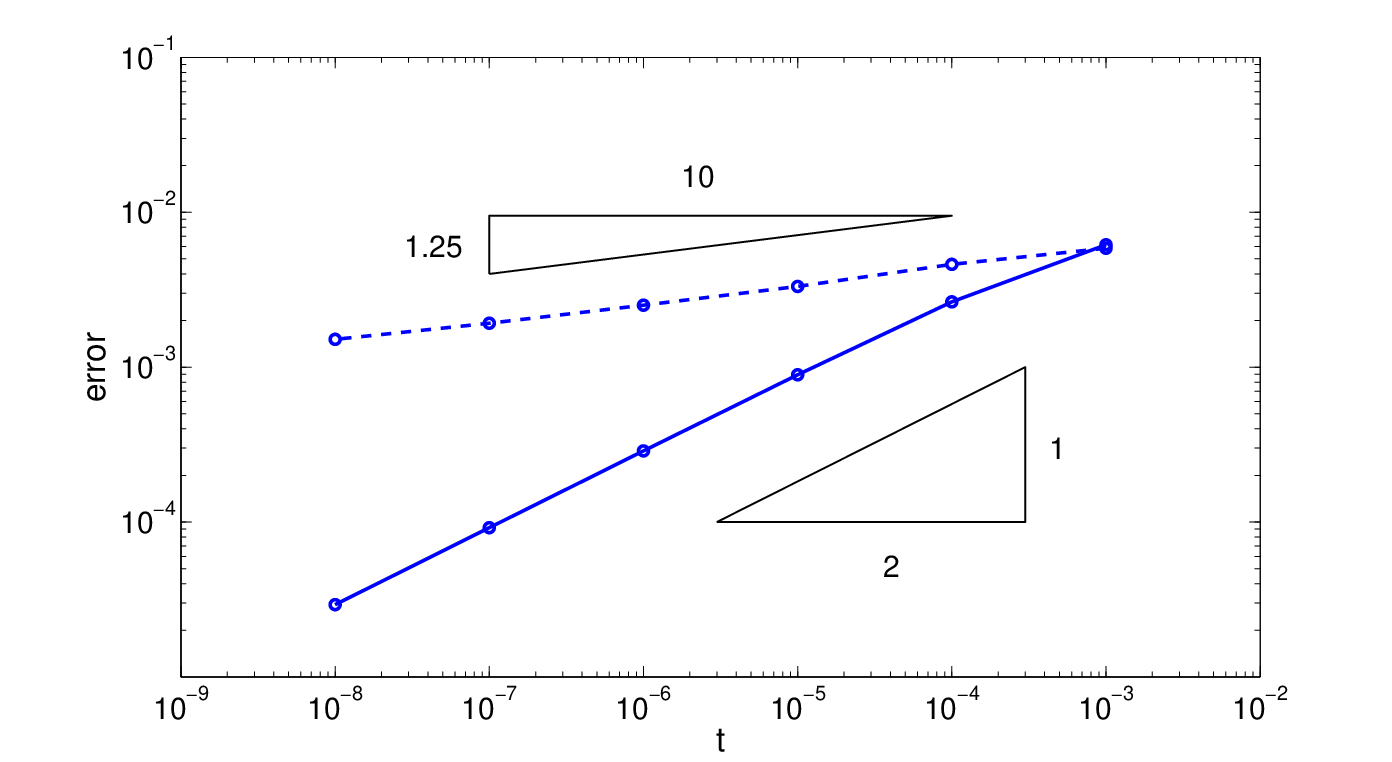
Last, we examine the inhomogeneous problem, i.e., case (c). The numerical results are given in Table 5, where the last two rows were obtained by correcting the right hand side , cf. (19). The BE scheme converges at the expected rate, but the SBD scheme only converges at a rate . The latter is attributed to the insufficient temporal regularity of the right hand side : only the first order derivative is integrable, but not high-order ones. One can also employ the correction in (19), which seems to restore the second-order convergence, cf. the last row of Table 5. However, the mechanism behind this remedy is still unknown.
4.2 Diffusion-wave equation
We consider the following four examples for the diffusion wave equation (with ):
- (d)
, and
- (e)
, and .
- (f)
, , .
- (g)
, , and .
Numerical results for examples (d) and (e)
First we briefly examine the convergence of the semidiscrete Galerkin scheme. The numerical results for cases (d) and (e) are shown in Fig. 2 and Table 6, respectively. We observe a convergence rate and in the - and -norm, respectively, for both smooth and nonsmooth data. For nonsmooth data, the error deteriorates as approaches zero, due to the weak singularity of the solution at close to zero, cf. Theorem 10, which we examine more closely next by verifying the prefactors in Theorem 3. For the smooth case (d), the error essentially stays unchanged with time , whereas for the nonsmooth case (e) it deteriorates like as , cf. Table 7. These observations agree well with the theory: by Theorem 2, as , there holds for any
Hence, the numerical results fully confirm the error estimates in Theorem 2.
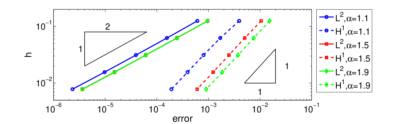
| rate | |||||||
|---|---|---|---|---|---|---|---|
| -norm | 1.51e-1 | 4.00e-3 | 1.00e-3 | 2.40e-4 | 4.83e-5 | 2.05 (2.00) | |
| -norm | 3.27e-1 | 1.40e-1 | 6.51e-2 | 3.11e-2 | 1.39e-2 | 1.10 (1.00) | |
| -norm | 5.71e-2 | 2.74e-2 | 9.29e-3 | 2.44e-3 | 5.07e-4 | 1.92 (2.00) | |
| -norm | 3.06e0 | 2.42e0 | 1.31e0 | 6.94e-1 | 2.55e-1 | 1.04 (1.00) | |
| -norm | 9.87e-2 | 4.32e-2 | 1.64e-2 | 4.94e-3 | 1.07e-3 | 1.78 (2.00) | |
| -norm | 6.86e0 | 4.60e0 | 2.87e0 | 1.37e0 | 5.72e-1 | 1.00 (1.00) |
| 1e-1 | 1e-2 | 1e-3 | 1e-4 | 1e-5 | rate | ||
|---|---|---|---|---|---|---|---|
| (d) | 1.66e-7 | 3.99e-6 | 5.14e-5 | 1.41e-4 | 9.16e-5 | 8.71e-5 | 0.02 (0) |
| (e) | 1.17e-7 | 2.58e-6 | 1.07e-4 | 1.69e-4 | 9.94e-4 | 6.04e-3 | -0.78 (-0.83) |
| (f) | 3.71e-6 | 1.50e-5 | 3.68e-6 | 2.83e-6 | 1.33e-6 | 5.40e-7 | 0.22 (0.18) |
Next we examine temporal convergence. The numerical results for case (d) are given in Table 8. The rates and are observed for the BE and SBD schemes, respectively, and they hold also for case (e), cf. Table 9. Hence, the proposed schemes exhibit a steady convergence for both smooth and nonsmooth data, verifying their robustness, cf. Theorems 5(ii) and 8(ii). Note that if the spatial error is negligible, then for fixed and , (30) holds, by Theorem 5(ii), which allows one to verify the temporal regularity in Theorem 11. In Table 10, we present the results for the BE scheme for . The -norm of the error decays at a rate for (d) and for (e), respectively, as , which concurs with the theoretical ones, thereby confirming the factor in Theorem 5(ii).
In Tables 8 and 9, we present also the results by the Crank-Nicolson (CN) scheme, which converges at a rate for solutions [48]. It achieves the desired rate in either case, even though by Theorem 11, the solution does not have the requisite regularity. These observations call for further analysis of the scheme.
| rate | ||||||||
|---|---|---|---|---|---|---|---|---|
| BE | 2.90e-2 | 1.49e-2 | 7.57e-3 | 3.81e-3 | 1.91e-3 | 9.59e-4 | 1.00 (1.00) | |
| SBD | 6.35e-4 | 2.02e-4 | 5.49e-5 | 1.41e-5 | 3.45e-6 | 7.50e-7 | 2.06 (2.00) | |
| CN | 3.40e-4 | 7.17e-5 | 1.44e-5 | 2.55e-6 | 2.62e-7 | 1.52e-7 | 2.36(1.90) | |
| BE | 4.53e-3 | 2.43e-3 | 1.26e-3 | 6.44e-4 | 3.26e-4 | 1.64e-4 | 0.99 (1.00) | |
| SBD | 1.25e-3 | 3.26e-4 | 8.22e-5 | 2.03e-5 | 4.51e-6 | 6.72e-7 | 2.06 (2.00) | |
| CN | 1.21e-3 | 4.41e-4 | 1.59e-4 | 5.72e-5 | 2.09e-5 | 7.83e-6 | 1.45(1.50) | |
| BE | 9.64e-3 | 4.91e-3 | 2.48e-3 | 1.24e-3 | 6.23e-4 | 3.11e-4 | 1.00 (1.00) | |
| SBD | 4.41e-4 | 1.25e-4 | 3.38e-5 | 8.58e-6 | 2.10e-6 | 7.66e-7 | 2.00 (2.00) | |
| CN | 8.06e-3 | 3.83e-3 | 1.80e-3 | 8.46e-4 | 3.95e-4 | 1.84e-4 | 1.10 (1.10) |
| rate | ||||||||
|---|---|---|---|---|---|---|---|---|
| BE | 2.16e-2 | 1.09e-2 | 5.47e-3 | 2.74e-3 | 1.37e-3 | 6.86e-4 | 1.00 (1.00) | |
| SBD | 3.47e-3 | 8.04e-4 | 1.94e-4 | 4.76e-5 | 1.17e-5 | 2.76e-6 | 2.02 (2.00) | |
| CN | 8.66e-2 | 2.62e-2 | 1.47e-3 | 1.69e-5 | 4.21e-6 | 9.67e-7 | 2.06 (1.90) | |
| BE | 3.82e-2 | 2.10e-2 | 1.11e-2 | 5.76e-3 | 2.93e-3 | 1.48e-3 | 1.00 (1.00) | |
| SBD | 1.18e-2 | 2.78e-3 | 6.64e-4 | 1.61e-4 | 3.92e-5 | 9.02e-6 | 2.06 (2.00) | |
| CN | 1.00e-2 | 2.66e-3 | 9.90e-4 | 3.60e-4 | 1.29e-4 | 4.58e-5 | 1.50 (1.50) | |
| BE | 1.11e-1 | 7.73e-2 | 5.15e-2 | 3.25e-2 | 1.93e-2 | 1.09e-2 | 0.83 (1.00) | |
| SBD | 7.36e-2 | 4.11e-2 | 1.85e-2 | 5.96e-3 | 1.56e-3 | 3.88e-4 | 1.95 (2.00) | |
| CN | 6.76e-2 | 4.42e-2 | 2.68e-2 | 1.51e-2 | 7.92e-3 | 3.95e-3 | 1.00 (1.10) |
| 1e0 | 1e-1 | 1e-2 | 1e-3 | 1e-4 | 1e-5 | rate | |
|---|---|---|---|---|---|---|---|
| (d) | 4.44e-4 | 6.33e-4 | 5.93e-5 | 1.82e-6 | 7.94e-8 | 3.97e-9 | 1.30 (1.10) |
| (e) | 2.56e-4 | 3.46e-3 | 1.35e-3 | 7.35e-4 | 3.77e-4 | 4.28e-5 | 0.32 (0.28) |
| (f) | 3.21e-5 | 1.06e-4 | 6.09e-6 | 3.04e-7 | 1.58e-8 | 5.42e-10 | 1.32 (1.28) |
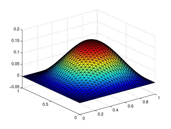
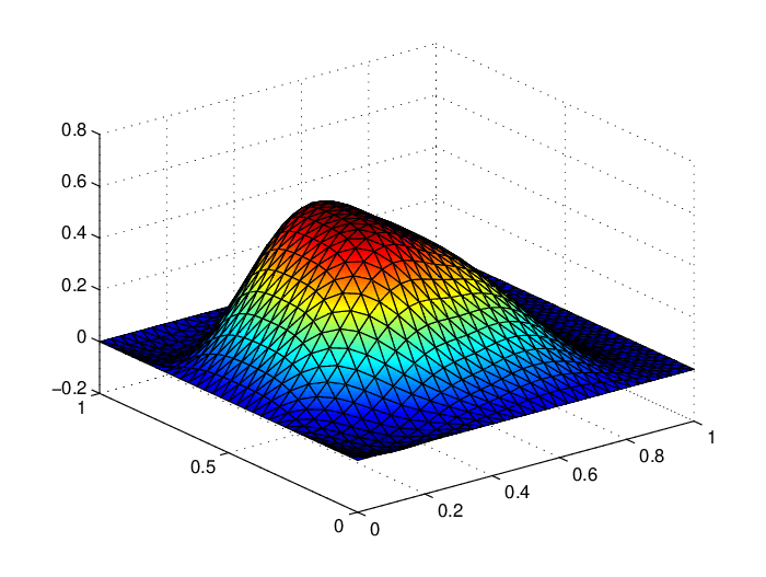
It is known that as the fractional order increases from one to two, the model (1) changes from a diffusion equation to a wave one [11]. This transition can be observed numerically: for close to one, the solution is diffusive and very smooth, whereas for close to two, the plateau in the initial data is well preserved, reflecting a “finite” speed of wave propagation, cf. Fig. 3. The small oscillations in Fig. 3 are not numerical artifacts: the projection is oscillatory, and the numerical solution inherits the feature. Further, the closer is to two, the slower is the decay of the solution (for close to zero), showing again the wave feature.
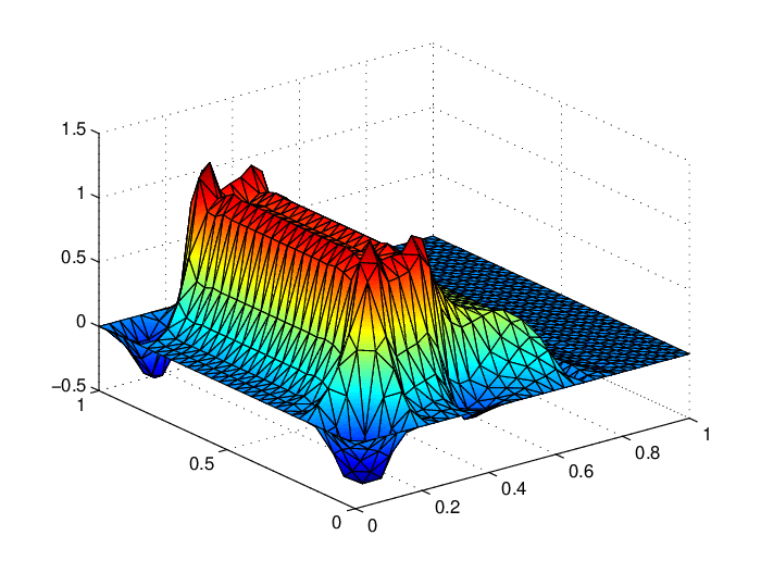
Numerical results for example (f)
Similar to cases (d) and (e), we observe the expected and convergence for the - and -norm of the error, respectively, cf. Fig. 4. An and convergence for the BE and SBD scheme, respectively, is observed, cf. Table 11. To examine more closely the solution singularity, we appeal to Theorem 5(ii) to deduce that for fixed
Hence, if the temporal error is negligible, the formula predicts a decay as . Since for case (f), for small , it predicts for , which is confirmed by the last row of Table 7. Likewise, if the spatial error is negligible, for fixed , the formula predicts a decay as . For , it predicts a rate , which agrees well with the last row of Table 10. These results confirm the error estimate in Theorem 5(ii).

method rate BE 1.12e-3 5.73e-4 2.90e-4 1.46e-4 7.30e-5 3.66e-5 1.00 (1.00) SBD 1.07e-4 2.54e-5 6.20e-6 1.53e-6 3.76e-7 8.83e-8 2.04 (2.00) BE 2.82e-3 1.46e-3 7.48e-4 3.78e-4 1.90e-4 9.53e-5 0.99 (1.00) SBD 2.37e-4 6.47e-5 1.65e-5 4.11e-6 1.01e-7 2.30e-8 2.02 (2.00) BE 3.65e-3 2.04e-3 1.11e-3 5.94e-4 3.12e-4 1.61e-4 0.94 (1.00) SBD 1.02e-3 4.13e-4 1.42e-4 4.06e-5 1.05e-5 2.93e-6 1.89 (2.00)
Numerical results for example (g)
Now we present numerical results for case (g) in Table 12, where the first and last two rows are for the basic and the corrected schemes, respectively. For the BE scheme, both variants (18) and (19) can achieve the desired convergence, and the errors are comparable. However, for the SBD scheme, the basic variant converges only at a suboptimal rate . It concurs with Theorem 9(i), since the right hand side is not regular enough. The correction indeed restores the desired convergence rate. These observations clearly show the crucial role of proper initial correction in high-order schemes, and in particular, an inadvertent implementation can compromise the accuracy.
| method | rate | |||||
|---|---|---|---|---|---|---|
| BE (18) | 4.20e-4 | 2.20e-4 | 1.14e-4 | 5.81e-5 | 2.97e-5 | 0.96 (1.00) |
| SBD (basic) | 2.40e-4 | 9.25e-5 | 3.66e-5 | 1.45e-5 | 5.43e-6 | 1.36 () |
| BE (19) | 4.71e-4 | 2.43e-4 | 1.24e-4 | 6.25e-5 | 3.14e-5 | 0.99 (1.00) |
| SBD (22) | 7.64e-5 | 1.92e-5 | 4.77e-6 | 1.17e-6 | 2.73e-7 | 2.04 (2.00) |
5 Conclusions
In this paper we develop two robust fully discrete schemes for the subdiffusion and diffusion wave equations. The schemes employ a Galerkin finite element method in space and the convolution quadrature generated by the backward Euler method and second-order backward difference. We provide a complete error analysis of the schemes, and derive optimal error estimates for both smooth and nonsmooth initial data. In particular, the schemes achieve a first-order and second-order convergence in time. We present extensive numerical experiments to illustrate the accuracy and robustness of the schemes. The experimental findings fully verify the convergence theory. Further, we compare our schemes with several existing time stepping schemes developed for smooth solutions, and find that existing ones may be not robust with respect to data regularity.
There are several questions deserving further investigation. First, in view of the solution singularity for nonsmooth data, it is of much practical interest to develop time stepping schemes using a nonuniform mesh in time and provide rigorous error analysis, including a posterior analysis. Second, our experiments indicate that existing time stepping schemes may yield only suboptimal convergence for nonsmooth data. This motivates revisiting these schemes for nonsmooth data, especially sharp error estimates. Last, it is important to study more complex models, e.g., variable coefficients in time and nonlinear models. The case of time dependent coefficients represents one of the major challenges in applying convolution quadrature, due to a lack of complete solution theory and loss of convolution structure.
Acknowledgements
The authors are grateful to the anonymous referees for their constructive comments. The research of B. Jin is partly supported by UK Engineering and Physical Sciences Research Council grant EP/M025160/1.
Appendix A The solution theory for the diffusion-wave equation
In the convergence analysis, the regularity of the solution to problem (1) plays an important role. The solution theory for with nonsmooth data is now well understood [45, 19, 18, 16]. Below we describe briefly the theory for following these works. Using the Dirichlet eigenpairs of the negative Laplacian , the solution to problem (1) with is given by
where the operators , and are given by , , , respectively, where the Mittag-Leffler function is defined by , [23, pp. 42]. It satisfies the following differentiation formula
| (31) |
and the following asymptotics: for [23, pp. 43]
| (32) |
First we give a stability result for the homogeneous problem.
Theorem 10.
Proof.
The next result gives temporal regularity for the homogeneous problem.
Theorem 11.
If , , , and , then for
Proof.
Now we turn to inhomogeneous problems. We have the following stability result.
Theorem 12.
For problem (1) with and , , there holds for any
Proof.
Last we state a temporal regularity result for the inhomogeneous problem.
Theorem 13.
If , and , then there holds
| (33) |
Proof.
Like before, the solution to the semidiscrete scheme (8) is given by
where the operators , and are given by , , , respectively, with being the eigenpairs of the discrete Laplacian . Then the following discrete counterpart of Theorem 10 holds, where denotes the discrete norm defined on , induced by [19]. The proof is identical with that for Theorem 10 and hence omitted.
Theorem 14.
The solution to problem (8) with satisfies for and
References
- [1] E Eric Adams and Lynn W. Gelhar, Field study of dispersion in a heterogeneous aquifer: 2. spatial moments analysis, Water Res. Research, 28 (1992), pp. 3293–3307.
- [2] Dumitru Baleanu, Kai Diethelm, Enrico Scalas, and Juan J. Trujillo, Fractional Calculus, World Scientific, Hackensack, NJ, 2012.
- [3] Emilia Bazhlekova, Bangti Jin, Raytcho Lazarov, and Zhi Zhou, An analysis of the Rayleigh–Stokes problem for a generalized second-grade fluid, Numer. Math., 131 (2015), pp. 1–31.
- [4] Chang-Ming Chen, Fawang Liu, I Turner, and V Anh, A Fourier method for the fractional diffusion equation describing sub-diffusion, J. Comput. Phys., 227 (2007), pp. 886–897.
- [5] Feng Chen, Qinwu Xu, and Jan S. Hesthaven, A multi-domain spectral method for time-fractional differential equations, J. Comput. Phys., 293 (2015), pp. 157–172.
- [6] Sheng Chen, Jie Shen, and Li-Lian Wang, Generalized Jacobi functions and their applications to fractional differential equations, Math. Comput., (2015), p. in press.
- [7] Eduardo Cuesta, Christian Lubich, and Cesar Palencia, Convolution quadrature time discretization of fractional diffusion-wave equations, Math. Comp., 75 (2006), pp. 673–696.
- [8] Kai Diethelm, The Analysis of Fractional Differential Equations, Lecture Notes in Mathematics, Springer, 2004.
- [9] Neville J. Ford, Jingyu Xiao, and Yubin Yan, A finite element method for time fractional partial differential equations, Fract. Calc. Appl. Anal., 14 (2011), pp. 454–474.
- [10] Hiroshi Fujita and Takashi Suzuki, Evolution problems, in Handbook of Numerical Analysis, Vol. II, Handb. Numer. Anal., II, North-Holland, Amsterdam, 1991, pp. 789–928.
- [11] Yasuhiro Fujita, Integrodifferential equation which interpolates the heat and the wave equation, Osaka J. Math., 27 (1990), pp. 309–321.
- [12] Guang-Hua Gao, Zhi-Zhong Sun, and Hong-Wei Zhang, A new fractional numerical differentiation formula to approximate the Caputo fractional derivative and its applications, J. Comput. Phys., 259 (2014), pp. 33–50.
- [13] Rudolf Gorenflo, Francesco Mainardi, Daniele Moretti, and Paolo Paradisi, Time fractional diffusion: a discrete random walk approach, Nonlin. Dyn., 29 (2002), pp. 129–143.
- [14] Ernst Hairer, Syvert P. Nørsett, and Gerhard Wanner, Solving Ordinary Differential Equations. I, Springer-Verlag, Berlin, second ed., 1993. Nonstiff Problems.
- [15] Yuko Hatano and Naomichi Hatano, Dispersive transport of ions in column experiments: An explanation of long-tailed profiles, Water Res. Research, 34 (1998), pp. 1027–1033.
- [16] Bangti Jin, Raytcho Lazarov, Joseph Pasciak, and Zhi Zhou, Galerkin FEM for fractional order parabolic equations with initial data in . LNCS 8236 (Proc. 5th Conf. Numer. Anal. Appl. (June 15-20, 2012)), Springer, pp. 24–37, 2013.
- [17] , Error analysis of a finite element method for the space-fractional parabolic equation, SIAM J. Numer. Anal., 52 (2014), pp. 2272–2294.
- [18] , Error analysis of semidiscrete finite element methods for inhomogeneous time-fractional diffusion, IMA J. Numer. Anal., 35 (2015), pp. 561–582.
- [19] Bangti Jin, Raytcho Lazarov, and Zhi Zhou, Error estimates for a semidiscrete finite element method for fractional order parabolic equations, SIAM J. Numer. Anal., 51 (2013), pp. 445–466.
- [20] , An analysis of the L1 scheme for the subdiffusion equation with nonsmooth data. IMA J. Numer. Anal., in press, 2015.
- [21] Bangti Jin and William Rundell, An inverse problem for a one-dimensional time-fractional diffusion problem, Inverse Problems, 28 (2012), pp. 075010, 19.
- [22] , A tutorial on inverse problems for anomalous diffusion processes, Inverse Problems, 31 (2015), pp. 035003, 40.
- [23] Anatoly A. Kilbas, Hari Mohan Srivastava, and Juan J. Trujillo, Theory and Applications of Fractional Differential Equations, Elsevier, Amsterdam, 2006.
- [24] T.A.M. Langlands and Bruce I. Henry, The accuracy and stability of an implicit solution method for the fractional diffusion equation, J. Comput. Phys., 205 (2005), pp. 719–736.
- [25] Changpin Li and Hengfei Ding, Higher order finite difference method for the reaction and anomalous-diffusion equation, Appl. Math. Model., 38 (2014), pp. 3802–3821.
- [26] Wulan Li and Da Xu, Finite central difference/finite element approximations for parabolic integro-differential equations, Computing, 90 (2010), pp. 89–111.
- [27] Xianjuan Li and Chuanju Xu, A space-time spectral method for the time fractional diffusion equation, SIAM J. Numer. Anal., 47 (2009), pp. 2108–2131.
- [28] Yumin Lin, Xianjuan Li, and Chuanju Xu, Finite difference/spectral approximations for the fractional cable equation, Math. Comp., 80 (2011), pp. 1369–1396.
- [29] Yumin Lin and Chuanju Xu, Finite difference/spectral approximations for the time-fractional diffusion equation, J. Comput. Phys., 225 (2007), pp. 1533–1552.
- [30] Christian Lubich, Discretized fractional calculus, SIAM J. Math. Anal., 17 (1986), pp. 704–719.
- [31] , Convolution quadrature and discretized operational calculus. I, Numer. Math., 52 (1988), pp. 129–145.
- [32] Christian Lubich, Ian H. Sloan, and Vidar Thomée, Nonsmooth data error estimates for approximations of an evolution equation with a positive-type memory term, Math. Comp., 65 (1996), pp. 1–17.
- [33] Francesco Mainardi, Fractional relaxation-oscillation and fractional diffusion-wave phenomena, Chaos, Solitons & Fractals, 7 (1996), pp. 1461–1477.
- [34] , Fractional Calculus and Waves in Linear Viscoelasticity, Imperial College Press, London, 2010.
- [35] William McLean, Regularity of solutions to a time-fractional diffusion equation, ANZIAM J., 52 (2010), pp. 123–138.
- [36] William McLean and Kassem Mustapha, Convergence analysis of a discontinuous Galerkin method for a sub-diffusion equation, Numer. Algor., 52 (2009), pp. 69–88.
- [37] William McLean and Vidar Thomée, Maximum-norm error analysis of a numerical solution via Laplace transformation and quadrature of a fractional-order evolution equation, IMA J. Numer. Anal., 30 (2010), pp. 208–230.
- [38] Elliott W Montroll and George H Weiss, Random walks on lattices. II, J. Math. Phys., 6 (1965), pp. 167–181.
- [39] Kassem Mustapha, Basheer Abdallah, and Khaled M. Furati, A discontinuous Petrov-Galerkin method for time-fractional diffusion equations, SIAM J. Numer. Anal., 52 (2014), pp. 2512–2529.
- [40] Kassem Mustapha and William McLean, Superconvergence of a discontinuous Galerkin method for fractional diffusion and wave equations, SIAM J. Numer. Anal., 51 (2013), pp. 491–515.
- [41] Kassem Mustapha and Dominik Schötzau, Well-posedness of -version discontinuous Galerkin methods for fractional diffusion wave equations, IMA J. Numer. Anal., 34 (2014), pp. 1426–1446.
- [42] Raoul R. Nigmatulin, The realization of the generalized transfer equation in a medium with fractal geometry, Phys. Stat. Sol. B, 133 (1986), pp. 425–430.
- [43] Keith B Oldham and Jerome Spanier, The Fractional Calculus, Academic Press, New York, 1974.
- [44] Igor Podlubny, Fractional Differential Equations, Academic Press, San Diego, CA, 1999.
- [45] Kenichi Sakamoto and Masahiro Yamamoto, Initial value/boundary value problems for fractional diffusion-wave equations and applications to some inverse problems, J. Math. Anal. Appl., 382 (2011), pp. 426–447.
- [46] Jesús María Sanz-Serna, A numerical method for a partial integro-differential equation, SIAM J. Numer. Anal., 25 (1988), pp. 319–327.
- [47] Hansjörg Seybold and Rudolf Hilfer, Numerical algorithm for calculating the generalized Mittag-Leffler function, SIAM J. Numer. Anal., 47 (2008/09), pp. 69–88.
- [48] Zhi-Zhong Sun and Xiaonan Wu, A fully discrete scheme for a diffusion wave system, Appl. Numer. Math., 56 (2006), pp. 193–209.
- [49] Vidar Thomée, Galerkin Finite Element Methods for Parabolic Problems, vol. 25 of Springer Series in Computational Mathematics, Springer-Verlag, Berlin, 2006.
- [50] Santos B. Yuste, Weighted average finite difference methods for fractional diffusion equations, J. Comput. Phys., 216 (2006), pp. 264–274.
- [51] Santos B. Yuste and Luis Acedo, An explicit finite difference method and a new von Neumann-type stability analysis for fractional diffusion equations, SIAM J. Numer. Anal., 42 (2005), pp. 1862–1874.
- [52] Fanhai Zeng, Changpin Li, Fawang Liu, and Ian Turner, The use of finite difference/element approaches for solving the time-fractional subdiffusion equation, SIAM J. Sci. Comput., 35 (2013), pp. A2976–A3000.