On the embedding of $A_{1}$ into $A_{\infty}$

The purpose of this article is to give a quantitative version of the classical embedding between Muckenhoupt classes

The class $A_{1}$ is defined to be all weights $w\geq 0$ for which $Mw\leq Cw$ for some $C$, where

is the uncentered Hardy-Littlewood maximal operator (here the supremum is taken over cubes with sides parallel to the coordinate axes).

The class $A_{\infty}$ is defined to be all weights $w\geq 0$ for which there exists a constant $C$ and an exponent $\epsilon>0$ such that

for all cubes $P$ and all subsets $E\subseteq P$. Another common way to define this class is to introduce the so-called Fujii-Wilson $A_{\infty}$ characteristic:

where the supremum ranges over cubes with sides parallel to the axes. The class of $A_{\infty}$ weights is the collection of all weights for which $[w]_{A_{\infty}}$ is finite.

These two definitions can be shown to be equivalent. In particular, one can give a quantitative version of the first:

With these definitions one can show that $[w]_{A_{\infty}}\sim_{d}[w]_{A_{\infty}^{\prime}}$. The easy direction is $[w]_{A_{\infty}}\lesssim_{d}[w]_{A_{\infty}^{\prime}}$, to prove the reverse inequality one can use the sharp reverse-Hölder estimate found in [3].

We are interested in this form of the $A_{\infty}$ characteristic because it is the one which is used some recent proofs of the weighted weak-type inequality for Calderón-Zygmund operators (see [2]), so it may yield some insights into the sharpness of such estimate. In fact, in the Bellman-function approach to the sharpness of this weak-type estimate, one has a very similar problem but with one extra difficulty; the problem treated in this article is the one which appears if this extra difficulty is removed, see [5] for more details.

It is a well-known fact that every weight in $A_{1}$ is also in $A_{\infty}$; here we give a quantitative version of this embedding.

We will actually work with a wider class of weights, the dyadic $A_{p}$ weights. To state the result, let us fix a way to quantify exactly how a weight lies in dyadic $A_{1}$. Let $P$ be a cube in $\mathbb{R}^{d}$, we define the $A_{1}^{d}(P)$ characteristic of a weight $w\geq 0$ to be

where $M^{\text{dyadic}}_{P}$ is the dyadic maximal operator localized to $P$:

Here we are denoting by $\mathcal{D}(P)$ the collection of all dyadic subcubes of $P$, and the average of a function $f$ over a set $E$ by

Also, we denote the characteristic function of a set $E$ by $\mathbbm{1}_{E}$.

We define the (non-dyadic) $A_{1}$ characteristic similarly:

where $M_{P}$ is the uncentered Hardy-Littlewood maximal operator where the cubes are constrained to lie inside $P$.

The classical way to prove (1.1) proceeds by using the reverse Hölder inequality of Coifman-Fefferman [1] (see [3] for a recent sharp reverse Hölder inequality valid in a very general context): for any weight $w\in A_{p}$ we have

for some exponent $q>1$ depending on $w$. Indeed, let $C_{\text{RH}}$ be the best constant in the above inequality (which will depend on $q$ and on how $w$ lies in $A_{p}$), then:

For (non-dyadic) $A_{1}$ weights the most quantitative version of the reverse Hölder inequality was given by [10] in dimension one. Using the results of [10] one obtains

for all $a>1$, so one can get arbitrarily close to the exponent $\frac{1}{[w]_{A_{1}}}$ at the cost of a multiplicative constant. The results in [10] are, however, valid only for non-dyadic $A_{p}$ weights, which behave much better in terms of sharp constants; also [10] is valid only in dimension $1$.

In [4] A. Melas showed that, for dyadic $A_{1}$ weights, one has

for all $p$ such that

and where $C(p,[w]_{A_{1}^{d}})$ is a constant which blows-up as $p$ tends to the endpoint above.

Following the same steps as before, this implies an inequality of the form

for all $\epsilon$ such that

and where $C_{\epsilon}$ is a constant which blows-up as $\epsilon$ tends to the endpoint $\epsilon([w]_{A_{1}^{d}},d)$.

It was of interest whether one could achieve an estimate with the endpoint $\epsilon([w]_{A_{1}^{d}},d)$, and this was answered positively by A. Osȩkowski in [7], where he proved the following weak-type estimate:

for all $p$ such that

This estimate, coupled with Hölder’s inequality for Lorentz spaces yields

for all weights $w$ with $[w]_{A_{1}^{d}}\leq Q$, thus settling the endpoint question of whether a decay rate of $(|E|/|P|)^{\epsilon(Q,d)}$ could be achieved. However, note that Hölder’s inequality for Lorentz spaces (when used in this way) has a constant which explodes when $p\to 1$ which in this case implies that the constant $C_{\epsilon(Q,d)}$ will blow-up as $Q\to\infty$.

In this article we improve this conclusion by directly computing the function

where the supremum is taken over all sets $E\subseteq P$ with $|E|/|P|=x$, and all dyadic $A_{1}$ weights $w$ with $[w]_{A_{1}^{d}(P)}\leq Q$, $\langle w\rangle_{P}=y$ and $\operatorname{ess\,inf}_{z\in P}w(z)=m$.

This is what is commonly called the Bellman function associated with the problem. It is an extremal object which controls the way in which the parameters evolve when “concatenating” several weights and sets together.

We can already give an upper bound for $\mathbb{B}(\cdot,Q,1)$:

This shows that the decay rate deduced from Osȩkowski’s estimate can be achieved with a uniform constant as $Q\to\infty$ (note that the constant $Q$ cancels when estimating $\frac{w(E)}{w(P)}$). Observe also that this recovers the result of Osȩkowski when one takes $w$ instead of its maximal function in (1.2), which can be interpreted as a weak-type reverse Hölder inequality. Indeed, assume without loss of generality that $|P|=\operatorname{ess\,inf}w=1$ and let $E_{\lambda}=\{x\in P:w(x)>\lambda\}$, then our estimate will show (see (4.1)) that

So integrating $w$ over this set yields

Or, in other words,

for the same $p$’s as in (1.2).

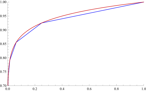
However, the function $\mathbb{B}(\cdot,Q,1)$ is, surprisingly, slightly better. Indeed if we define $f(x)=\mathbb{B}(x,Q,1)$, then our main result shows that $f$ is the piecewise-linear interpolation of the function $\widetilde{f}$ evaluated at the points $2^{-dk}$ for $k\in\mathbb{N}$.

In Figure 1 we show a normalized section of the plot (the values are divided by $Q$) of the functions $f$ and $\widetilde{f}$ with $Q=10$ and in dimension two.

The precise form of $\mathbb{B}$ is given in the following theorem, which is the main result of this article.

I wish to thank Professor Alexander Volberg for many invaluable discussions regarding Bellman functions. I also am greatly indebted to Professor Ignacio Uriarte-Tuero without whom this project could not have happened. I also benefited very much from discussions about this result with Professors David Cruz-Uribe, Leonid Slavin, and Vasily Vasyunin. Finally, I would like to thank Professor Cristina Pereyra for organizing the New Mexico Analysis Seminar, which provided the perfect environment for many stimulating discussions related to this work.

Define, as in the introduction, the function

By translation and dilation invariance, the function $\mathbb{B}_{P}$ is independent of $P$, so we suppress the index $P$ from $\mathbb{B}$ from now on.

The domain, which will be denoted by $\Omega_{\mathbb{B}}$ is:

In this section we cast finding $\mathbb{B}$ as a minimization problem. We will follow the Bellman function method, see for example [6], [10] or [9], and [7] for an approach closer to ours.

The function $\mathbb{B}$ satisfies the following Main Inequality

where $\langle x_{i}\rangle=x$, $\langle y_{i}\rangle=y$, $\min m_{i}=m$, $(x_{i},y_{i},m_{i})\in\Omega$, and $(x,y,m)\in\Omega$. In inequality (3.1), and for the rest of the article, we use the notation

whenever $\{\xi_{i}\}$ is a discrete sequence of $n$ numbers; usually $n$ will be obvious from the context so we will omit its dependence.

We can see (3.1) by combining almost-extremizers defined on the first-generation dyadic subcubes of $P$ into one on the whole cube $P$.

We also have the obstacle condition

which is just the observation that if $E=P$ almost everywhere, then $\langle\mathbbm{1}_{E}w\rangle_{P}=\langle w\rangle_{P}$.

From the definition of $\mathbb{B}$ we have the homogeneity property

If we find a nonnegative function $B$ defined in $\Omega_{\mathbb{B}}$ and which satisfies the main inequality and the obstacle condition above, then $\mathbb{B}\leq B$. This is a typical fact whose proof we omit, but the reader can consult [7] for a proof in a similar case.

The homogeneity condition will let us assume that $m=1$ in (3.1):

We want to find a set of necessary and sufficient conditions for $B$ to satisfy the main inequality, but which are simpler to verify. To this end, let us first prove necessary conditions that any such $B$ must satisfy.

The following Lemma is simple but important in what follows. It tells us that, in order to exploit (3.1), we should strive to minimize the variables $m_{i}$ as much as possible. We will let $N:=2^{d}$ for the rest of the article.

The following Lemma follows directly from the main inequality (3.1).

Now we are able to make the first reduction in (3.1) (after the trivial one of setting $m=1$):

This proposition is useful because it allows us to “almost” eliminate the third variable from our analysis. The reason that we used the word “almost” comes from the fact that we still have the extraneous condition that $\min(y_{i})\leq Q$, which is an effect of having $\min(m_{i})=1$. We now proceed to eliminate this condition too.

Suppose that of the $N$ points $(x_{i},y_{i})$, there are exactly $N-k$ of them for which $y_{i}\geq Q$. Then, after possibly reordering the inequality (which we can do without loss of generality), the right hand side of (3.4) becomes

which can be written, after applying the homogeneity property (3.2), as

So, verifying (3.4) reduces to just showing that $B$ is concave in $(x,y)$, decreasing in $m$, and that for each $1\leq k\leq N-1$

for all $(x,y)$ and all $(x_{i},y_{i})$ as in Proposition (3.4), with the additional assumption that $y_{i}\geq Q$ for $k\geq k+1$.

The next proposition allows us to just consider the case where $k=N-1$ in the above inequality.

In this section we give a lower bound $M$ for $\mathbb{M}$, and in the next section we will show that this lower bound is also an upper bound and hence that $M=\mathbb{M}$.

First recall that

is non-increasing and therefore that $\mathbb{M}(1,y)\geq y$ (here we are using the obstacle $\mathbb{M}(1,1)=1$. Since $\mathbb{M}(0,1)\geq 0$, we now can extend this bound to the subdomain $y\leq 1+(Q-1)x$ to get:

We will now give a lower bound for $\mathbb{M}$ in the rest of the domain. The idea is to use inequality (3.8) setting the number $Nx-(N-1)\widetilde{x}$ to be as large as possible, within the domain that we know, and then iterate.

More precisely let $x_{0}=1$, observe that if $Nx-(N-1)\widetilde{x}=x_{0}$, then

Clearly we need $x\geq 1/N$ for $\widetilde{x}$ to be in the domain, so we set $x=\frac{1}{N}$. We will also make $\widetilde{y}$ as small as possible, which means $\widetilde{y}=1$.

Putting it all together we obtain, using (3.8) with $x=\frac{1}{N}$ and $y=Q$:

Now we iterate this procedure. Set $x=x_{k+1}=\frac{x_{k}}{N}$, $y=Q$, $\widetilde{y}=1$ and $\widetilde{x}=0$, then (3.8) gives

so

Between $x_{k+1}$ and $x_{k}$ we know that $M(\cdot,Q)$ is concave, so $\mathbb{M}$ must certainly be at least linear in these intervals. Now, since $\mathbb{M}(0,1)\geq 0$, we can also extend this bound by homogeneity and get the upper bound

for $y-1\geq x$. Here, $f$ is the piecewise linear function defined on $[0,1]$ by linearly interpolating the points

between $x_{k+1}$ and $x_{k}$, Figure 1 shows what $f$ typically looks like.

Putting it all together, we get

The way we proved these bounds also shows how one would construct pairs of weights $w$ and sets $E$ showing that $\mathbb{M}$ is at least the promised lower bound. We now give a detailed description of these examples.

References

• [1] R. R. Coifman and C. Fefferman. Weighted norm inequalities for maximal functions and singular integrals. Studia Math., 51:241–250, 1974.
• [2] C. Domingo-Salazar, M. T. Lacey, and G. Rey. Borderline weak-type estimates for singular integrals and square functions. Bulletin of the London Mathematical Society, Dec. 2015.
• [3] T. Hytönen, C. Pérez, and E. Rela. Sharp reverse Hölder property for A∞A_{\infty} weights on spaces of homogeneous type. J. Funct. Anal., 263(12):3883–3899, 2012.
• [4] A. D. Melas. A sharp LpL^{p} inequality for dyadic A1A_{1} weights in ℝn\mathbb{R}^{n}. Bull. London Math. Soc., 37(6):919–926, 2005.
• [5] F. Nazarov, A. Reznikov, V. Vasyunin, and A. Volberg. A Bellman function counterexample to the A1A_{1} conjecture: the blow-up of the weak norm estimates of weighted singular operators. ArXiv e-prints, June 2015.
• [6] F. Nazarov, S. Treil, and A. Volberg. The Bellman functions and two-weight inequalities for Haar multipliers. J. Amer. Math. Soc., 12(4):909–928, 1999.
• [7] A. Osȩkowski. Sharp inequalities for dyadic A1A_{1} weights. Arch. Math. (Basel), 101(2):181–190, 2013.
• [8] G. Rey and A. Reznikov. Extremizers and sharp weak-type estimates for positive dyadic shifts. Adv. Math., 254:664–681, 2014.
• [9] L. Slavin, A. Stokolos, and V. Vasyunin. Monge-Ampère equations and Bellman functions: the dyadic maximal operator. C. R. Math. Acad. Sci. Paris, 346(9-10):585–588, 2008.
• [10] V. I. Vasyunin. The exact constant in the inverse Hölder inequality for Muckenhoupt weights. Algebra i Analiz, 15(1):73–117, 2003.