Generalized gradient approximation correlation energy functionals based on the uniform electron gas with gap model
Abstract
We study the uniform electron gas with a gap model in the context of density functional theory. Based on this analysis, we construct two local gap models that realize generalized gradient approximation (GGA) correlation functionals satisfying numerous exact constraints for the correlation energy. The first one, named GAPc, fulfills the full second-order correlation gradient expansion at any density regime, is very accurate for jellium surfaces, comparable to state-of-the-art GGAs for atomic systems and molecular systems, and well compatible with known semilocal exchange. The second functional, named GAPloc, is satisfying the same exact conditions, except that the second-order gradient expansion is sacrificed for a better behavior under the Thomas-Fermi scaling and a more realistic correlation energy density of the hellium atom. The GAPloc functional displays a high accuracy for atomic correlation energies, still preserving a reasonable behavior for jellium surfaces. Moreover, it shows a higher compatibility with the Hartree-Fock exchange than other semilocal correlation functionals. This feature is explained in terms of the real-space analysis of the GAPloc correlation energy.
I Introduction
Model systems play a prominent role in Kohn-Sham (KS) [1] density functional theory (DFT) [2], due to their utility in understanding and guiding the development of physically sound and accurate exchange-correlation (XC) functionals, which shall include quantum effects of the many-electron interaction. Thus, over the years, a wide number of model systems has been considered within DFT [1, 3, 4, 5, 6, 7, 8, 9, 10, 11, 12, 13, 14, 15, 16, 17, 18, 19, 20, 21, 22].
The first, and probably most important, model system of DFT has been the uniform electron gas [1] that is a paradigm for solid-state physics and most non-empirical XC functionals [23]. The uniform electron gas model leads straightforwardly to relatively simple explicit expressions for both the exchange and the correlation energy of a many electron system, within the so called local density approximation (LDA) [1, 24, 25, 26, 27]. This approximation, despite its simplicity, provides a remarkably good qualitative description of inhomogeneous electronic systems, however, it fails severely to yield accurate quantitative results.
For this reason many improvements over the LDA level of theory have been proposed [23]. In particular, by using the gradient of the density as an additional input ingredient, useful generalized gradient approximation [28] (GGA) functionals have been developed, which provide a good compromise between simplicity, computational efficiency, and numerical accuracy [5, 11, 29, 30, 31, 32, 33, 34, 35, 36, 37, 38, 39, 40, 41, 42, 43, 44, 45, 46, 47]. Alternatively, for the correlation energy, Rey and Savin [18] proposed to consider a model system (jellium with gap) obtained by adding a non-local one-body operator to the true Hamiltonian of the uniform electron gas, in order to force an arbitrary gap between occupied and virtual orbitals. In this way, in fact, the strong overestimation of the LDA correlation can be largely corrected. Moreover, for the jellium with gap model system the correlation energy can be computed with high accuracy for different values of . Then, an analytic representation of the LDA with gap correlation functional is readily available [18].
This formula can be easily extended to be used for inhomogeneous systems after providing, in analogy with the usual LDA approach, an appropriate local description of the gap (i.e. a function ). This idea was used as a seed to construct the KCIS [48] and KCISK [49] correlation functionals which showed, with their good performance, the advantages of the jellium with gap model system. However, in the construction of the KCIS/KCISK functional only a limited focus was posed on the local gap functional and a rather simple ansatz was used for the gap . In contrast, several important constraints of the exact correlation energy, were satisfied using the conventional approach of GGA and meta-GGA functionals. In particular, the LDA for the uniform electron gas at was substituted by a GGA expression to assure the recovery of the second-order gradient expansion for the correlation energy (only at ) [48, 49].
In this paper we want to resume the work on the jellium with gap correlation and explore the possibility to construct appropriate local gap models in order to achieve an accurate description of inhomogeneous electronic systems. In this sense, our work differs from the one performed for the KCIS/KCISK functionals [48, 49], because of the stronger attention we put on the construction of the local gap function. We show in fact that it is possible, in general, to recover many exact properties of the correlation energy by building a suitable local gap function , being a functional of the density and its gradient. The focus of our work will be on the GGA level of theory because, being this the most simple beyond LDA, it is also the most powerful for showing the significance of various exact conditions and for exploring and explaining the physics related to a particular model system. Thus, by developing two, conceptually different, local gap models, we aim at showing the power of this approach. At the same time, our functionals may be also considered the basis for more sophisticated developments, even beyond the GGA level. Nevertheless, in this paper we address only the GGA level and thus all our results are compared with the GGA state-of-the-art ones.
II Theory
Within the jellium with gap model [18, 49] the correlation energy is defined as
| (1) |
where is the electron density, is the local Seitz radius, is the relative spin polarization, is the gap, and
| (2) |
In Eq. (2) the spin mixing factor is
| (3) |
while the fully-spin-polarized () and the spin-unpolarized () correlation energies per particle have the form (the spin index is omitted hereafter for notational simplicity)
| (4) |
with being the conventional local density approximation for the correlation energy and , , and some density-dependent coefficients [18]. Full details about the construction of the model as well as its asymptotic properties are discussed in the appendix.
The main goal of this work is finding appropriate local gap functions (with and ), such that exact contraints of the correlation energy can be imposed to the jellium with gap model. The idea behind this approach is that the LDA model with a gap can accurately describe, at each point in space, the correlation energy per particle of an inhomogeneous electron distribution if a proper gap is applied at each point, depending on the local/semilocal properties of the electron densities at that point.
To this end, we consider in the appendix a detailed analysis of several known exact constraints for the correlation energy and their relation with local gap function. In particular we consider the uniform electron gas limit (), the slowly-varying density limit (), the rapidly-varying density limit (), the uniform scaling to the high-density limit [50], and the Thomas-Fermi scaling [9, 51]. Using this information we can propose two local gap functions able to enforce a set of exact constraints on the jellium with gap correlation.
With the aim of imposing the second-order gradient expansion behavior we consider the general formula of Eq. (35) and set
| (5) |
with
| (6) |
where is the -dependent second-order correlation coefficient of Hu and Langreth [52] (we use the parametrization of Ref. 53) and is a parameter fixed by minimizing the variance of the correlation energy error for the noble gas atoms He, Ne, and Ar. The resulting functional is labeled GAPc and satisfies all the exact constraints mentioned before (i.e. the uniform electron gas and the slowly-varying limits, the rapidly-varying density limit, the uniform scaling towards the high-density limit, and the Thomas-Fermi scaling behavior; see the appendix for details). Thus, it formally fulfills the same exact conditions as the PBE correlation functional [29]. However, the GAPc functional recovers the true second-order gradient expansion at any , whereas PBE does it only in the high-density limit. Moreover, in the tail of an atomic density , with , (note that ), therefore the GAPc functional has the tail decay , closer to the behavior described in Ref. 54 (note that ).
A second useful local gap function can be obtained by dropping the requirement that the second-order gradient expansion behavior is satisfied. This condition was shown in fact to be not very important for many cases [55]. In this way the choice of the local gap function is no more bound to Eq. (35) and a more flexible ansatz can be employed. Our choice, which defines the GAPloc functional is
| (7) |
where , , and
| (8) |
Note that ( being the von Weizsäker kinetic energy density [56]) is the local gap function used in the KCIS/KCISK functionals [48, 49]. The two parameters and were fixed by fitting to the exact correlation energy per particle of the He atom (i.e. the function reported in Ref. 57). We recall that fitting to the energy density of model systems is a common practice in DFT, used for instance in the construction of the AM05 [37, 38] and ARPA+ [5] GGA functionals, which may help to reduce the error cancellation effects in contrast to fitting to integrated energies. The GAPloc functional satisfies the following exact constraints:
(1) LDA limit; in fact for we have . Note however that for the functional behaves as
| (9) |
Thus, as anticipated, the GAPloc functional does not recover the second-order gradient expansion behavior but approaches the LDA limit much faster.
(2) Rapidly-varying density limit; for and finite, and the correlation correctly vanishes.
(3) Uniform scaling to the high density-limit; in this limit . Thus, according to Eq. (36) and the logarithmic divergence of LDA is canceled.
(4) Thomas-Fermi scaling; in fact in this limit we have
| (10) |
and for any positive .
The tail behavior of the GAPloc functional can be also easily inspected noting that in the tail of an atomic density , with (see appendix). Thus, the local gap function behaves as
| (11) |
where is weakly dependent on . Equation (11) indicates that as then therefore the GAPloc functional (a.i. ) decays as . However, because the actual value of the parameter is rather large this asymptotic behavior is set only quite far in the tail, whereas at smaller distances the local gap function is quite bigger. As a consequence the GAPloc correlation energy per particle will decrease rather fast in the outer valence region and then attains a decay behavior in the far tail.
The different features of the GAPc and GAPloc functionals that we discussed above are summarized in Figure 1 where we report a plot of the correlation energy densities for several values of and and compare them with the the PBE functional. Similar plots are obtained for the KCIS/KCISK correlation energy densities.
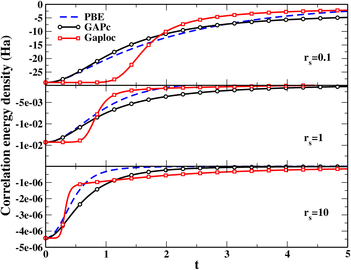
The figure highlights in particular the similarity of the GAPc and PBE functionals for small and small , because both functionals recover the same second-order gradient expansion in this high-density limit. The similarity is much less for larger values of the Seitz parameter, because in this case the PBE functional fails to recover the correct value of . Another important feature that emerges from the plot is the peculiar shape of the GAPloc functional. In fact, as discussed above, this functional recovers the LDA limit for a much broader interval of small values but then shows a sudden reduction of the correlation energy density at before starting a slow decay. This behavior corresponds, despite the slow asymptotic decay behavior, to a localization of the correlation energy density near the atomic nuclei. This is an important feature of this functional that will be discussed in more details later.

Finally, we show in Fig. 2, the opposite of the radial correlation energy density () versus the radial distance for the He atom. By construction, GAPloc is very close to the exact curve. Note instead that a functional that recovers the second-order gradient expansion in general can not be accurate near the nucleus, giving a too small (in absolute value) correlation energy density at small . Then, assuming that this functional is accurate for the total correlation energy (), it must give a too large (in absolute value) correlation energy density at larger . Hence, such a correlation energy density is quite different from the exact behavior, being modified up to a gauge transformation [58]. Such a gauge had been the subject of intense research, at the hyper-GGA level of theory [59]. Both PBE and GAPc show this semilocal-gauge behavior, while PBEloc [16] is definitely better due to the localization concept which incorporates [16]. Note also that GAPc is slightly worse than PBE (and very similar to revTPSS instead), because it recovers the full (correct) second-order gradient expansion and its total correlation energy () is slightly worse (see Table 1).
III Computational details
To test the correlation functionals we performed several calculations on different test sets that are summarized below. We remark that the selection of tests for the assessment of the GAPc functional in conjunction with the revPBE exchange [30] was restricted to those properties and systems where the revPBE exchange may be expected to yield reasonable results [60] (e.g. atomization energies of organic molecules, atomic properties). We did not consider instead tests where the revPBE exchange is completely inadequate (e.g. structural properties, metallic systems, solids), because in these cases it would be impossible to extract any useful information on the performance of the correlation, which is the target of the present study, due to the dominating exchange error.
The following sets of properties were considered
- •
- •
Jellium surface correlation energies. We compared the surface correlation energies of semi-infinite jellium surfaces with bulk parameter , 3, 4, and 6. Reference data were taken from diffusion Monte Carlo (DMC) calculations [65].
- •
- •
- •
Other properties We considered the G21P set of ionization potentials of atoms and molecules [70, 71], the EA13 test of electron affinities of atoms and molecules [72], the PA13 set comprising proton affinities of organic molecules [70], and the AE17 test set of atomic non-relativistic exchange-correlation energies [73]. In addition, we tested the HB6 set of hydrogen-bond complexes [74].
Molecular calculations were carried out self-consistently with the TURBOMOLE program package [75] using the def2-TZVPP basis set [76, 77]. Atomic calculations for Table 1 were performed using a cc-pV5Z basis set [78, 79, 80, 81]. Atomic calculations for Fig. 3 were carried out with the Engel code [82], using accurate exact exchange orbitals and densities. Jellium calculations were performed with numerical Kohn-Sham LDA orbitals and densities. FORTRAN90 routines implementing both functionals are freely available on the web [83].
IV Numerical results
In this section we report the results of some numerical calculations that we performed to assess the performance of the correlation functionals and study their properties in different contexts.
IV.1 Atomic and jellium correlation energies
Table 1 reports the correlation energy per electron of several atoms and ions as computed with different correlation functionals.
| System | LDA | LYP | PBE | APBE | GAPc | GAPloc | Ref. | |
|---|---|---|---|---|---|---|---|---|
| He | 2 | -56.2 | -21.9 | -21.0 | -18.7 | -26.2 | -20.0 | -21.0 |
| Li+ | 2 | -67.3 | -23.8 | -22.4 | -19.8 | -27.6 | -20.4 | -21.7 |
| Be2+ | 2 | -75.2 | -24.5 | -23.0 | -20.3 | -28.0 | -20.0 | -22.2 |
| Li | 3 | -50.3 | -17.8 | -17.1 | -15.2 | -21.4 | -15.9 | -15.1 |
| Be+ | 3 | -57.6 | -20.4 | -18.1 | -15.9 | -22.3 | -16.1 | -15.8 |
| B2+ | 3 | -63.2 | -22.3 | -18.6 | -16.3 | -22.7 | -15.8 | -16.2 |
| C3+ | 3 | -67.7 | -23.7 | -18.9 | -16.6 | -22.9 | -15.5 | -16.5 |
| N4+ | 3 | -71.5 | -24.8 | -19.1 | -16.7 | -22.9 | -15.2 | -16.7 |
| O5+ | 3 | -74.9 | -25.6 | -19.2 | -16.8 | -22.8 | -14.9 | -16.8 |
| Ne7+ | 3 | -80.4 | -26.9 | -19.4 | -16.9 | -22.7 | -14.4 | -17.0 |
| Ar15+ | 3 | -94.9 | -29.2 | -19.7 | -17.1 | -22.2 | -13.9 | -17.4 |
| Be | 4 | -56.0 | -23.6 | -21.4 | -19.3 | -25.7 | -20.2 | -23.6 |
| B+ | 4 | -63.0 | -26.7 | -23.0 | -20.8 | -27.4 | -21.7 | -27.8 |
| C2+ | 4 | -68.5 | -28.6 | -24.0 | -21.6 | -28.4 | -22.3 | -35.1 |
| N3+ | 4 | -73.0 | -30.0 | -24.7 | -22.2 | -29.0 | -23.0 | -35.1 |
| O4+ | 4 | -76.9 | -30.9 | -25.3 | -22.7 | -29.4 | -23.7 | -38.5 |
| N | 7 | -61.0 | -27.4 | -25.7 | -23.4 | -28.8 | -25.8 | -26.9 |
| O+ | 7 | -65.6 | -29.5 | -27.0 | -24.5 | -29.9 | -27.0 | -27.7 |
| Ne | 10 | -74.3 | -38.4 | -35.1 | -32.3 | -38.2 | -38.5 | -39.1 |
| Ar8+ | 10 | -96.8 | -44.9 | -41.0 | -37.6 | -42.0 | -45.0 | -39.9 |
| Ar6+ | 12 | -90.2 | -44.8 | -38.3 | -35.0 | -40.1 | -40.8 | -41.3 |
| Ar | 18 | -79.1 | -41.7 | -39.3 | -36.4 | -41.0 | -43.0 | -40.1 |
| Zn | 30 | -88.5 | -47.7 | -46.9 | -43.6 | -47.3 | -52.6 | -56.2 |
| Kr | 36 | -90.8 | -48.6 | -49.1 | -45.8 | -48.8 | -56.1 | -57.4 |
| ME | -44.1 | -1.6 | 2.0 | 4.6 | -1.4 | 2.6 | ||
| MAE | 44.1 | 4.8 | 3.8 | 4.6 | 4.9 | 3.4 | ||
| MARE | 192% | 21% | 13% | 13% | 21% | 11% | ||
| St. Dev. | 11.8 | 5.8 | 5.0 | 5.1 | 5.5 | 4.7 |
All the GGA functionals reported in the table perform rather similarly and improve considerably over the LDA functional. Nevertheless, the best results are obtained by the GAPloc functional which yields a mean absolute error (MAE) of 3.4 mHa and a mean absolute relative error of 11%. Slightly larger errors are yielded by the PBE functional. All other GGAs here are roughly 1 mHa worst on average. In particular, the GAPc functional gives a MAE of 4.9 mHa, slightly better than the LYP functional. Note also that KCIS performs similarly to PBE (MAE 3.8 kcal/mol), whereas KSICK yields results comparable to GAPloc (MAE 3.3 kcal/mol).
These results are extrapolated to larger atoms in Fig. 3 where we report the correlation energy per electron of atoms up to Fr () as computed with different functionals. We remark that in this case the comparison is only semi-quantitative, because highly accurate benchmark results are missing for heavier atoms. Nevertheless, good reference data are obtained by the virial-constrained effective Hamiltonian (VCEH) method [63].

The plot confirms the remarkable accuracy of the GAPloc functional even for heavy atoms. At the same time it shows that the GAPc functional is comparable in accuracy with the PBE correlation over the whole periodic table of elements. This result can be rationalized considering that in fact the two functionals are constructed by imposing the same exact constraints. Moreover, it supports the idea of using the jellium with gap model as a reference system to describe the correlation energy of inhomogeneous electron systems.
To complete our assessment we report in Table 2 jellium surface correlation energies calculated with different methods and compare them with accurate diffusion Monte Carlo (DMC) results [65].
| LDA | PBE | PBEloc | GAPc | GAPloc | DMC | |
| 2 | 318 | 829 | 773 | 725 | 665 | 768 50 |
| 3 | 95 | 276 | 251 | 233 | 229 | 242 10 |
| 4 | 39 | 124 | 112 | 103 | 105 | 104 8 |
| 6 | 10 | 40 | 35 | 31 | 33 | 31 |
| MAE | 171 | 31 | 7 | 13 | 30 | |
| MARE | 62.4% | 17.6% | 6.2% | 2.6% | 6.5% |
The best results in this case are obtained by the GAPc functional which yields for any results in agreement with the reference DMC values and the best MARE (it also gives the second best MAE; note anyway that the low MAE of PBEloc is mostly due to its extremely good performance for , while in the other cases GAPloc has lower or equal absolute errors). Thus, for the jellium surface correlation energies the GAPc functional definitely outperforms the PBE functional. This traces back to the fact that the former recovers the correct second-order gradient expansion coefficient at any while the latter only in the high-density limit. In fact, for GAPc the relative errors are almost constant at any value of the bulk parameter, while for PBE they increase significantly with . Interestingly, the GAPc functional shows also a better overall performance than the PBEloc functional, which was parametrized on the jellium surface correlation energies.
Concerning the GAPloc functional we note that it displays a remarkably good performance, being even better than PBE (same MAE but better MARE) and roughly comparable with the PBEloc functional, especially at larger values (larger MAE but same MARE). This result is an important achievement for the GAPloc functional since it was constructed disregarding the satisfaction of the second-order gradient expansion and, even more importantly, because for a quite wide range of values around zero it recovers very closely LDA, which is indeed very bad for this problem. Nonetheless, we recall that the correct behavior in the slowly-varying limit is not the only important feature in the description of jellium surface energies, because this problem also shows important contributions from the rapidly-varying regions that are present outside the surface. Thus, the crucial ingredient for the accurate calculation of jellium surface energies is the correct balance of the two limits. This balance appears to be well described by the GAPloc functional which thus yields reasonably accurate results for jellium surface correlation energies.
Finally, we recall that KCISK meta-GGA correlation functional improves over the KCIS meta-GGA correlation functional, for jellium surface correlation energies, but it is slightly worse than the PBE functional (see Fig. 6 and Table 4 of Ref. 49).
IV.2 Performance in combination with exchange
To test further the capabilities of the correlation functionals we considered their use with exchange. To this end, at first we tested several combinations of our correlation with existing GGA exchange functionals. We found that the GAPc functional is rather well compatible with the revPBE exchange [30]. On the other hand, no good exchange counterpart was found for the GAPloc functional, probably because the peculiar form of this functional requires ad hoc features in the exchange part which are not included in present semilocal functionals. Nevertheless, the GAPloc functional was found to be well compatible with Hartree-Fock exchange. Thus, we additionally considered a set of tests of our correlation functionals in combination with the exact Hartree-Fock exchange. We remark that, since the focus of the present paper is on correlation functionals based on the jellium with gap model, the testing within a XC approach has the only scope to demonstrate the possible compatibility of the present correlation methods in such a scheme, whereas the development of an optimal semilocal exchange for the GAPc and especially the GAPloc functionals is left for future work. At the same time the use of the functionals in combination with Hartree-Fock exchange is only intended to show the actual compatibility of the methods with the exact exchange, without any intention to solve more subtle problems related to static correlation or non-local effects (see also Ref. 16).
| Test | LDA | BLYP | PBE | APBE | revPBE | X+GAPc |
|---|---|---|---|---|---|---|
| AE6 | 75.6 | 6.8 | 14.2 | 7.8 | 9.0 | 6.2∗ |
| W4 | 44.0 | 5.8 | 10.7 | 8.6 | 6.7 | 6.9 |
| TM10AE | 29.7 | 13.8 | 12.8 | 11.5 | 10.7 | 12.2 |
| BH6 | 18.0 | 8.2 | 9.4 | 8.3 | 6.8 | 5.6∗ |
| K9 | 14.6 | 6.0 | 7.3 | 6.5 | 4.9 | 4.9∗ |
| DC9 | 156.9 | 26.5 | 40.8 | 29.4 | 34.2 | 24.9∗ |
| G21IP | 4.8 | 4.8 | 3.9 | 4.0 | 4.2 | 2.8∗ |
| EA13 | 3.4 | 9.5 | 7.4 | 7.5 | 8.7 | 6.0∗ |
| PA13 | 4.3 | 2.4 | 2.2 | 2.8 | 4.0 | 4.1 |
| AE17 | 426.5 | 7.4 | 51.6 | 22.2 | 13.6 | 11.6∗ |
| ARDPBE | 3.14 | 0.82 | 1.00 | 0.85 | 0.86 | 0.75∗ |
In Table 3 we report the mean absolute errors of several tests on atoms and molecules as resulting from different GGA approaches. The functional obtained by the combination of revPBE exchange and GAPc correlation has been labeled X+GAPc. In the last line we report the average relative deviation with respect to PBE (ARDPBE) defined as
| (12) |
where denotes the MAE of any given method for the -th test. This indicator provides a fair overall assessment of the whole set of tests [60, 84, 85, 86].
We remark that the set of tests in Table 3 does not provide, nor is intended to provide, a throughout assessment of the functionals but aims instead at demonstrating the compatibility of the GAPc functional with semilocal exchange over a rather broad range of problems. This compatibility is indeed well evident by inspecting the results reported in Table 3. In fact, the X+GAPc functional shows a performance comparable with that of the best GGA XC functionals (BLYP [31, 32] and APBE [11]). More importantly, the comparison between revPBE and X+GAPc results shows that the latter are in general superior to the former, despite the exchange part was not optimized for use with GAPc. In particular, we remark the important improvement for ionization potentials (G21IP), and electron affinities (EA13) since these properties may be closely related to opening of a gap in the the jellium with gap model system. This indicates the goodness of the GAPc correlation and suggest that it can be a promising tool for future development of a semilocal XC functional.
As additional test we report in Table 4 the performance of several GGA correlation functionals in combination with Hartree-Fock exchange for a selected set of properties (see also Ref 16).
| Hartree-Fock + | |||||
|---|---|---|---|---|---|
| Test | LYP | PBE | PBEloc | GAPc | GAPloc |
| AE6 | 38.2 | 31.9 | 24.0 | 33.5 | 23.1 |
| BH6 | 5.3 | 5.6 | 4.4 | 6.1 | 3.7 |
| K9 | 6.0 | 5.7 | 4.7 | 6.0 | 3.4 |
| HB6 | 2.3 | 1.5 | 1.7 | 1.4 | 1.3 |
Inspection of the table shows that, as discussed above, the GAPloc functional is definitely more compatible with Hartree-Fock exchange that other GGA functionals, outperforming for all the tests considered also the PBEloc correlation [16] which was constructed to enhance such compatibility. As we will show in next subsection, the good results of the GAPloc functional in this context may be possibly traced back to its ability to describe with good accuracy the correlation energy density of different systems so that it can be summed to the Hartree-Fock energy density, which is long-range, with small error accumulation (see also next subsection). For this reason the functional can yield also very accurate integrated correlation energies (see Table 1). Possibly for the same reason the GAPloc functional is hardly compatible with existing semilocal exchange approximations, because these provide a too poor description of long-range effects (that in common XC functionals are probably described by the correlation part). In fact, in our tests the GAPloc correlation showed a reasonable performance in combination with a PBE-like exchange functional [29] with enhancement factor only for very large values of , i.e. when a high nonlocality is introduced into the functional [60]. Finally, we remark the good performance of HF+GAPloc for the kinetics (K9 test), being better than GGAs, many meta-GGAs [84], and hybrids functionals [86].
Finally, we mention that both KCIS and KCISK correlation functionals are well compatible with semilocal exchange. Thus, the PKZB meta-GGA exchange [87] combined with KCISK is accurate for atomization energies of small molecules [49], while TPSS exchange [88] combined with KCIS correlation gives good results for many properties [89].
IV.3 Real-space analysis of GAPloc
The results of Table 4 show that GAPloc has a higher compatibility with Hartree-Fock exchange. We argued that this property depends on the good shape of its correlation energy density. In order to understand better this point we perform in this subsection the real-space analysis [2, 90] of the GAPloc correlation
| (13) |
where is a spin index, is the number of electrons with spin and the angle- and system-averaged correlation hole is
| (14) |
with the solid angle element in the -space. The coupling-constant averaged correlation hole is constructed using the reverse-engineering method of Ref. 91 (see the Appendix). Note that the quantity has the dimension of a spherically-averaged energy density and its analysis allows to inspect the physical content of a given functional with high accuracy by comparison with accurate reference benchmarks. The correlation hole is in fact not only a space-resolved expansion of the correlation energy, but unlike the correlation energy density is uniquely defined [92]. Moreover, we recall that, at full coupling strength, the correlation hole is an observable [92]. We must stress anyway that while the PBE correlation hole was constructed entirely from physical exact conditions, the reverse engineering method used in the construction of the GAPloc correlation hole is not unique, depending on the GAPloc correlation energy density. However, the here proposed GAPloc hole satisfies important exact conditions (e.g. hole sum rule, energy sum rule, accurate LDA on-top hole, and RPA non-oscillatory long-range contribution; see appendix and Ref. 91), and thus it can be seen as a practical tool which reveals the physics behind the GAPloc correlation functional. We also recall that the TPSS and PBE correlation holes of Refs. 94, 92, 93 are very well mimicked by the reverse engineering hole method (see Fig. 2 of Ref. 91) inside of the Coulomb hole radius.

In Fig. 4 we report the real-space analysis of the GAPloc correlation energy for several atoms and ions. The PBE and PBEloc as well reference curves are also reported for comparison. The plot shows that overall the GAPloc functional provides a better description of the correlation hole, in particular at short range which is the most relevant for any semilocal functional (whereas the long-range part can be hardy described accurately at this level of theory). On the other hand, at longer range the GAPloc plots, similarly to PBE, show some cusp features due to the cutoff procedure used to ensure the proper normalization of the hole during its construction [91, 92] (see Eq. (47)). On the contrary PBEloc displays smoother hole curves because, thanks to its very rapid decay in the tail of the density, the cuttoff procedure is better averaged in the process of real-space calculation.
One more important observation is that the GAPloc functional describes reasonably well also the larger atoms, i.e. Na+ and Ne, giving a good and balanced description of all the features of their correlation hole. This is a remarkable achievement of the GAPloc functional, since other GGA functionals, and even meta-GGA ones [91], perform rather worse in this context.
To make the analysis more quantitative we report in Table 5 the Coulomb hole radius as obtained from the different GGA holes. We recall that the Coulomb hole radius is the smallest distance () where the correlation hole equals zero. This is an important quantity to define the effect of correlation on the distribution of the electrons in the vicinity of each other [91, 96].
| Atom | LDA | PBE | PBEloc | GAPloc | Ref. |
|---|---|---|---|---|---|
| He | 3.51 | 1.32 | 0.97 | 1.00 | 0.93 |
| Li+ | 2.53 | 0.84 | 0.67 | 0.63 | 0.67 |
| Be2+ | 2.06 | 0.62 | 0.51 | 0.45 | 0.49 |
| B3+ | 1.77 | 0.49 | 0.42 | 0.35 | 0.35 |
| Ne8+ | 1.15 | 0.25 | 0.23 | 0.16 | 0.17 |
| Ca18+ | 0.78 | 0.13 | 0.12 | 0.08 | 0.08 |
| Li | 2.53 | 0.85 | 0.67 | 0.63 | 0.67 |
| Be | 5.23 | 0.65 | 0.54 | 0.46 | 0.48 |
| Ne | 2.35 | 1.21 | 1.04 | 1.11 | 1.27 |
| Na+ | 2.05 | 1.10 | 0.92 | 0.94 | 0.98 |
| MAE | 1.79 | 0.15 | 0.06 | 0.04 | |
| MARE | 420% | 32% | 15% | 5% |
The data in the table confirm that the GAPloc functional is the most accurate for the description of the Coulomb hole, with a MAE of 0.04 Bohr and a MARE of 5%. Note that this is a remarkable performance, even outperforming meta-GGA functionals [91]. Good results are found also with the PBEloc correlation functional which yields a MAE of 0.06 Bohr, similar to the BLOC meta-GGA correlation functional [84, 91]. Note that the PBE functional displays also a good performance, greatly improving over the LDA, but still shows a systematic overestimation of the Coulomb hole radius.
V Conclusions
In this paper we have studied the jellium with gap model in the context of the ground-state density functional theory. First, we have proposed a reparametrization of the spin-dependence of the jellium with gap correlation energy (in the spirit of the Perdew-Wang LDA correlation parametrization, see Table 6). Next, we derived exact constraints for the local gap function, starting from known exact properties of the correlation energy. This analysis allowed us to construct two semilocal correlation functionals, namely GAPc and GAPloc, that keep the original jellium with gap functional form and are characterized solely by the modelling of the local gap function .
The GAPc functional recovers the correct second-order gradient expansion at any density, satisfies various density-scaling properties, and has a slower decay in the tail of the density than the PBE functional (see Fig. 1). It is well compatible with the revPBE exchange functional, which is considered one of the most accurate semilocal exchange, improving the total MAE of various properties and test sets with about 15% (see Table 3). It competes with state-of-the-art GGA functionals for the correlation energies of atoms and ions (see Table 1), while outperforms them for the jellium surface correlation energies (see Table 2), suggesting that it can be a useful tool for solid-state physics if combined with a proper semilocal exchange.
The GAPloc functional satisfies various density-scaling properties, and recovers the LDA functional over a wide range of slowly-varying regimes. This later feature is a direct consequence of the fitting to the exact correlation energy density of He atom. It is very accurate for total correlation energies of atoms and ions (see Table 1), performs reasonably well for jellium surface correlation energies (see Table 2), and is one of the most compatible GGA correlation functionals with the exact exchange (see Table 4). Moreover, by constructing its underlying correlation hole, we have shown that it gives the most realistic real-space analysis of the atomic correlation energy (see Fig. 4), and Coulomb hole radii (see Table 5). These results suggest that GAPloc can be also used in construction of more sophisticated functionals (e.g. hybrids and hyper-GGAs).
Finally, we mention that this work provides indications that the second-order gradient expansion of the correlation energy introduces a gauge in the correlation energy density which is not compatible with the exact exchange, but it is with semilocal exchange. Thus, it is responsable for an important part of the exchange-correlation error compensation.
Appendix A Local density approximation with a gap and its asymptotic properties
The main equation defining the LDA with gap model is Eq. (4). This uses as main ingredients the convetional LDA correlation energy per particle, here in the Perdew-Wang parametrization [27],
| (15) | |||||
and the functions , , and are
| (16) |
| (17) |
| (18) |
where
| (19) |
| (20) |
| (21) |
The numerical values of all the parameters, for both the spin-unpolarized and the fully-spin-polarized case, are reported in Table 6. Note that with respect to Ref. 49 for the fully-spin-polarized case we performed a reparametrization of , , and in order to remove the prefactors from the definition of , , . This makes the formulas for and formally identical and simplifies the notation. Our fit agrees with the results of Ref. 49 within 0.1 mHa (note that this is one order of magnitude smaller than the accuracy of the original fit).
In the low-density limit ( and ) the functions , , and behave as
| (22) |
| (23) |
| (24) |
Thus, we have for the spin-polarized and -unpolarized correlation energies per particle
| (25) |
On the other hand, in the high-density limit, when and we have
| (26) | |||||
| (27) | |||||
| (28) |
Therefore, the spin-polarized and -unpolarized correlation energies per particle behave as
| (29) |
A.1 Exact constraints for the local gap function
Several exact constraints are known for the correlation energy and can be used to construct accurate approximate correlation functionals with minimal empiricism. In this subsection we investigate how these constraints apply to the LDA model with a gap and, in particular, we consider the corresponding requirements for a local gap function .
A.1.1 Uniform electron gas and slowly-varying density limits
In the limit of the uniform electron gas () we must have . Thus, we must require that the gap vanishes wherever , i.e. we must impose that with .
In the slowly-varying density limit () the correlation energy per particle is described by the second-order gradient expansion [29, 100]
| (30) |
with the (eventually -dependent) second-order gradient expansion correlation coefficient [101, 52]. To fulfill the second-order gradient expansion any functional must satisfy the condition
| (31) |
Using the chain rule
| (32) |
we thus find
| (33) | |||||
This condition cannot be easily satisfied for any , without a strong modification of Eq. (2). Nevertheless, it can be easily satisfied in both the spin-unpolarized and the full-spin-polarized limits, yielding the condition
| (34) |
The uniform electron gas limit and Eq. (34) are fulfilled by a local gap function of the general form
| (35) |
where and .
A.1.2 Rapidly-varying density limit
A.1.3 Uniform scaling to the high-density limit
Under the uniform scaling to the high-density limit [50] with . Thus, as and as . In this limit the correlation energy per particle must scale to a constant [29, 102]. However, the LDA correlation is diverging logarithmically [27].
According to Eq. (29), under the uniform scaling to the high-density limit, the fully-spin-polarized and the spin-unpolarized correlation energies per particle of the jellium with gap model behave as
| (36) |
To cancel the logarithmic divergence of the LDA correlation we must therefore require that or diverges faster than .
In the first case, for the local gap function of Eq. (35) we must have
| (37) |
This condition is satisfied by
| (38) |
A.1.4 Thomas-Fermi scaling
The Thomas-Fermi scaling [9, 51] is defined by the transformation with . Hence, as , while is unchanged. Under this scaling the semiclassical high-density limit is reached. In this condition the correlation is dominated by the LDA contribution [51], thus it must scale as .
When the Thomas-Fermi scaling is set up, according to Eq. (29), the fully-spin-polarized and the spin-unpolarized correlation energies per particle of the jellium with gap model behave as
| (39) |
Thus, to achieve the proper scaling the local gap function must behave in this limit as with .
For the local gap function of Eq. (35) this condition implies
| (40) |
Hence, we must have that is not diverging faster than .
A.1.5 Tail behavior
Although there are no exact constraints known for the behavior of the correlation energy per particle in the tail of atomic systems it is interesting to investigate the decay of correlations functionals in this situation. In fact, recent work highlighted the importance of the tail behavior for approximate correlation functionals [16].
In the tail of an atom the electron density has the asymptotic form [103]
| (41) |
with the energy of the highest occupied orbital. Thus, of course . The reduced gradient for correlation is consequently
| (42) |
Therefore, both the Seitz radius and the square of the reduced gradient for correlation show the same decay behavior in the tail of an atom. We formalize this situation by introducing a scaling parameter such that and .
The behavior of the fully-polarized and unpolarized correlation energies per particle in this regime is described by Eq. (25). We see that for any local gap function not vanishing faster than the decay behavior of the correlation energies per particle is
| (43) |
Note that in contrast the decay behavior of the PBE correlation functional is [16]
| (44) |
where
| (45) |
with a constant. Thus, in the tail of an atomic density we have
| (46) |
Appendix B GGA hole model
In Ref. 91 the reverse engineering hole model was shown for the most general case of meta-GGA functionals. Here we report explicit formulas for the GGA case. The spin- and angle-averaged correlation hole model is
| (47) | |||||
where is the reduced electron-electron separation on the scale of the screening length. The function is the LDA correlation hole [92, 104]. The function is chosen to be
| (48) | |||||
Here is the RPA nonoscilating long-range contribution [92], is a scaled distance suitable for the gradient correction, with measuring where the short range contribution vanishes. The function is fixed by imposing the energy sum rule . It is
| (49) | |||||
This function controls the short-range (small ) behavior of the hole model, which is the most important for a semilocal hole. In contrast with the case of Ref. 92, it is not constructed from the slowly-varying behavior of any underlying functional, but it is instead entirely determined by the energy sum rule. Therefore, it is more general and can be used to any semilocal correlation functional.
References
- [1] Kohn. W.; Sham, L. Phys. Rev. 1965, 140, A1133.
- [2] Parr, R. G.; Yang, W. Density-Functional Theory of Atoms and Molecules; Oxford University Press: Oxford, 1989.
- [3] Kohn, W.; Mattsson, A. E. Phys. Rev. Lett. 1998, 81, 3487–3490.
- [4] Vitos, L.; Johansson, B.; Kollár, J.; Skriver, H. L. Phys. Rev. B 2000, 62, 10046–10050.
- [5] Constantin, L. A.; Ruzsinszky, A.; Perdew, J. P. Phys. Rev. B 2009, 80, 035125.
- [6] Constantin, L. A.; Ruzsinszky, A. Phys. Rev. B 2009, 79, 115117.
- [7] Solomatin, A.; Sahni, V. Phys. Rev. B 1997, 56, 3655–3658.
- [8] Lang, N. D.; Kohn, W. Phys. Rev. B 1970, 1, 4555–4568.
- [9] Elliott, P.; Lee, D.; Cangi, A.; Burke, K. Phys. Rev. Lett. 2008, 100, 256406.
- [10] Lee, D.; Constantin, L. A.; Perdew, J. P.; Burke, K. J. Chem. Phys. 2009, 130, 034107.
- [11] Constantin, L. A.; Fabiano, E.; Laricchia, S.; Della Sala, F. Phys. Rev. Lett. 2011, 106, 186406.
- [12] Pollack, L.; Perdew, J. P. J. Phys.: Condens. Matter 2000, 12, 1239.
- [13] Constantin, L. A. Phys. Rev. B 2008, 78, 155106.
- [14] Chiodo, L.; Constantin, L. A.; Fabiano, E.; Della Sala, F. Phys. Rev. Lett. 2012, 108, 126402.
- [15] Filippi, C.; Umrigar, C. J.; Taut, M. J. Chem. Phys. 1994, 100, 1290.
- [16] Constantin, L. A.; Fabiano, E.; Sala, F. D. Phys. Rev. B 2012, 86, 035130.
- [17] Hao, F.; Armiento, R.; Mattsson, A. E. Phys. Rev. B 2010, 82, 115103.
- [18] Rey, J.; Savin, A. Int. J. Quant. Chem. 1998, 69, 581–590.
- [19] Trevisanutto, P. E.; Terentjevs, A.; Constantin, L. A.; Olevano, V.; Della Sala, F. Phys. Rev. B 2013, 87, 205143.
- [20] Pittalis, S.; Räsänen, E.; Marques, M. A. L. Phys. Rev. B 2008, 78, 195322.
- [21] Janesko, B. G.; Aguero, A. J. Chem. Phys. 2012, 136, 024111.
- [22] Tognetti, V.; Cortona, P.; Adamo, C. Chem. Phys.Lett. 2008, 460, 536 – 539.
- [23] Scuseria, G. E.; Staroverov, V. N. In Theory and Applications of Computational Chemistry: The First 40 Years (A Volume of Technical and Historical Perspectives); Dykstra, C. E., Frenking, G., Kim, K. S., Scuseria, G. E., Eds.; Elsevier: Amsterdam, 2005; Chapter 24, p 669-724.
- [24] Dirac, P. A. M. Proc. Royal Soc. A 1929, 123, 714.
- [25] Slater, J. C. Phys. Rev. 1951, 81, 385–390.
- [26] Vosko, S. H.; Wilk, L.; Nusair, M. Can. J. Phys. 1980, 58, 1200–1211.
- [27] Perdew, J. P.; Wang, Y. Phys. Rev. B 1992, 45, 13244–13249.
- [28] Langreth, D. C.; Mehl, M. J. Phys. Rev. B 1983, 28, 1809–1834.
- [29] Perdew, J. P.; Burke, K.; Ernzerhof, M. Phys. Rev. Lett. 1996, 77, 3865–3868.
- [30] Zhang, Y.; Yang, W. Phys. Rev. Lett. 1998, 80, 890–890.
- [31] Becke, A. D. Phys. Rev. A 1988, 38, 3098–3100.
- [32] Lee, C.; Yang, W.; Parr, R. G. Phys. Rev. B 1988, 37, 785–789.
- [33] Fabiano, E.; Constantin, L. A.; Della Sala, F. Phys. Rev. B 2010, 82, 113104.
- [34] Constantin, L. A.; Fabiano, E.; Della Sala, F. Phys. Rev. B 2011, 84, 233103.
- [35] Constantin, L. A.; Fabiano, E.; Sala, F. D. J. Chem. Phys. 2012, 137, 194105.
- [36] Fabiano, E.; Constantin, L. A.; Sala, F. D. J. Chem. Phys. 2011, 134, 194112.
- [37] Armiento, R.; Mattsson, A. E. Phys. Rev. B 2005, 72, 085108.
- [38] Mattsson, A. E.; Armiento, R. Phys. Rev. B 2009, 79, 155101.
- [39] Pittalis, S.; Räsänen, E.; Vilhena, J. G.; Marques, M. A. L. Phys. Rev. A 2009, 79, 012503.
- [40] del Campo, J. M.; Gázquez, J. L.; Trickey, S.; Vela, A. Chem. Phys. Lett. 2012, 543, 179 – 183.
- [41] Vela, A.; Pacheco-Kato, J. C.; Gázquez, J. L.; del Campo, J. M.; Trickey, S. B. J. Chem. Phys. 2012, 136, 144115.
- [42] del Campo, J. M.; Gázquez, J. L.; Trickey, S. B.; Vela, A. J. Chem. Phys. 2012, 136, 104108.
- [43] Tognetti, V.; Cortona, P.; Adamo, C. Chem. Phys. Lett. 2007, 439, 381 – 385.
- [44] Tognetti, V.; Adamo, C.; Cortona, P. Interdiscip. Sci.: Comput. Life Sci. 2010, 2, 163–168.
- [45] Tognetti, V.; Cortona, P.; Adamo, C. Int. J. Quant. Chem. 2010, 110, 2320–2329.
- [46] Brémond, E.; Pilard, D.; Ciofini, I.; Chermette, H.; Adamo, C.; Cortona, P. Theor. Chem. Acc. 2012, 131, 1–7.
- [47] Brémond, E.; Kalhor, M.; Bousquet, D.; Mignon, P.; Ciofini, I.; Adamo, C.; Cortona, P.; Chermette, H. Theor. Chem. Acc. 2013, 132, 1–12.
- [48] Krieger, J. B.; Chen, J.; Iafrate, G. J.; A., S. In Electron Correlations and Materials Properties; Gonis, A., Kioussis, N., Ciftan, M., Eds.; Kluwer Academic: New York, 1999; pp 463–477.
- [49] Krieger, J. B.; Chen, J.; Kurth, S. AIP Conference Proceedings 2001, 577, 48-69.
- [50] Görling, A.; Levy, M. Phys. Rev. A 1992, 45, 1509–1517.
- [51] Fabiano, E.; Constantin, L. A. Phys. Rev. A 2013, 87, 012511.
- [52] Hu, C. D.; Langreth, D. C. Phys. Rev. B 1986, 33, 943–959.
- [53] Perdew, J. P.; Ruzsinszky, A.; Csonka, G. I.; Constantin, L. A.; Sun, J. Phys. Rev. Lett. 2009, 103, 026403; Phys. Rev. Lett. 2011, 106, 179902.
- [54] Almbladh, C.-O.; von Barth, U. Phys. Rev. B 1985, 31, 3231–3244.
- [55] Pedroza, L. S.; da Silva, A. J. R.; Capelle, K. Phys. Rev. B 2009, 79, 201106.
- [56] von Weiszsäcker, C. F. Z. Phys. 1935, 96, 431.
- [57] Baerends, E. J.; Gritsenko, O. V. J. Phys. Chem. A 1997, 101, 5383–5403.
- [58] Tao, J.; Staroverov, V. N.; Scuseria, G. E.; Perdew, J. P. Phys. Rev. A 2008, 77, 012509.
- [59] Perdew, J. P.; Staroverov, V. N.; Tao, J.; Scuseria, G. E. Phys. Rev. A 2008, 78, 052513.
- [60] Fabiano, E.; Constantin, L. A.; Della Sala, F. J. Chem. Theory Comput. 2011, 7, 3548–3559.
- [61] Constantin, L. A.; Chiodo, L.; Fabiano, E.; Bodrenko, I.; Della Sala, F. Phys. Rev. B 2011, 84, 045126.
- [62] Davidson, E. R.; Hagstrom, S. A.; Chakravorty, S. J.; Umar, V. M.; Fischer, C. F. Phys. Rev. A 1991, 44, 7071–7083.
- [63] Clementi, E.; Corongiu, G. Int. J. Quant. Chem. 1997, 62, 571–591.
- [64] McCarthy, S. P.; Thakkar, A. J. J. Chem. Phys. 2011, 134, 044102.
- [65] Wood, B.; Hine, N. D. M.; Foulkes, W. M. C.; Garcia-González, P. Phys. Rev. B 2007, 76, 035403.
- [66] Lynch, B. J.; Truhlar, D. G. J. Phys. Chem. A 2003, 107, 8996–8999.
- [67] Karton, A.; Tarnopolsky, A.; Lameère, J.-F.; Schatz, G. C.; Martin, J. M. L. J. Phys. Chem. A 2008, 112, 12868–12886.
- [68] Lynch, B. J.; Truhlar, D. G. J. Phys. Chem. A 2003, 107, 3898–3906.
- [69] Peverati, R.; Truhlar, D. G. J. Chem. Theory Comput. 2012, 8, 2310–2319.
- [70] Goerigk, L.; Grimme, S. J. Chem. Theory Comput. 2010, 6, 107–126.
- [71] Goerigk, L.; Grimme, S. Phys. Chem. Chem. Phys. 2011, 13, 6670–6688.
- [72] Lynch, B. J.; Zhao, Y.; Truhlar, D. G. J. Phys. Chem. A 2003, 107, 1384–1388.
- [73] Zhao, Y.; Truhlar, D. Theor. Chem. Acc. 2008, 120, 215–241.
- [74] Zhao, Y.; Truhlar, D. G. J. Chem. Theory Comput. 2005, 1, 415–432.
- [75] TURBOMOLE V6.2, 2009, a development of University of Karlsruhe and Forschungszentrum Karlsruhe GmbH, 1989-2007, TURBOMOLE GmbH, since 2007; available from http://www.turbomole.com; accessed on 13.03.2014.
- [76] Weigend, F.; Furche, F.; Ahlrichs, R. J. Chem. Phys. 2003, 119, 12753.
- [77] Weigend, F.; Ahlrichs, R. Phys. Chem. Chem. Phys. 2005, 7, 3297–3305.
- [78] Woon, D. E.; Dunning, T. H. J. Chem. Phys. 1994, 100, 2975.
- [79] Woon, D. E.; Dunning, T. H. J. Chem. Phys. 1993, 98, 1358.
- [80] Dunning, T. H. J. Chem. Phys. 1989, 90, 1007.
- [81] Balabanov, N. B.; Peterson, K. A. J. Chem. Phys. 2005, 123, 064107.
- [82] Engel, E. In A Primer in Density Functional Theory; Fiolhais, C., Nogueira, F., Marques, M. A. L., Eds.; Springer: Berlin, 2003; pp 56–122.
- [83] FORTRAN90 routines are freely available at http://www.theory-nnl.it/software.php; accessed on 13.03.2014.
- [84] Constantin, L. A.; Fabiano, E.; Della Sala, F. J. Chem. Theory Comput. 2013, 9, 2256–2263.
- [85] Laricchia, S.; Fabiano, E.; Constantin, L. A.; Della Sala, F. J. Chem. Theory Comput. 2011, 7, 2439–2451.
- [86] Fabiano, E.; Constantin, L. A.; Della Sala, F. Int. J. Quant. Chem. 2013, 113, 673–682.
- [87] Perdew, J. P; Kurth, S.; Zupan, A.; Blaha, P. Phys. Rev. Lett. 1999, 82, 2544.
- [88] Tao, J.; Perdew, J. P.; Staroverov, V. N.; Scuseria, G. E. Phys. Rev. Lett. 2003, 91, 146401.
- [89] Zhao Y.; Truhlar, D. G. J. Phys. Chem. A 2005, 109, 5656.
- [90] Becke, A. D. J. Chem. Phys. 1988, 88, 1053.
- [91] Constantin, L. A.; Fabiano, E.; Della Sala, F. Phys. Rev. B 2013, 88, 125112.
- [92] Perdew, J. P.; Burke, K.; Wang, Y. Phys. Rev. B 1996, 54, 16533–16539.
- [93] Pitarke, J. M.; Constantin, L. A.; Perdew, J. P. Phys. Rev. B 2006, 74, 045121.
- [94] Constantin, L. A.; Perdew, J. P.; Tao, J. Phys. Rev. B 2006, 73, 205104.
- [95] Cioslowski, J.; Liu, G. J. Chem. Phys. 1998, 109, 8225.
- [96] Slamet, M.; Sahni, V. Phys. Rev. A 1995, 51, 2815–2825.
- [97] O’Neill, D. P.; Gill, P. M. W. Phys. Rev. A 2003, 68, 022505.
- [98] Katriel, J.; Roy, S.; Springborg, M. J. Chem. Phys. 2005, 123, 104104.
- [99] Coulson, C. A.; Neilson, A. H. Proc. Phys. Soc. 1961, 78, 831.
- [100] Wang, Y.; Perdew, J. P. Phys. Rev. B 1991, 43, 8911–8916.
- [101] Ma, S.-K.; Brueckner, K. A. Phys. Rev. 1968, 165, 18–31.
- [102] Levy, M. Int. J. Quant. Chem. 1989, 36, 617–619.
- [103] Levy, M.; Perdew, J. P.; Sahni, V. Phys. Rev. A 1984, 30, 2745–2748.
- [104] Perdew, J. P.; Wang, Y. Phys. Rev. B 1992, 46, 12947–12954.